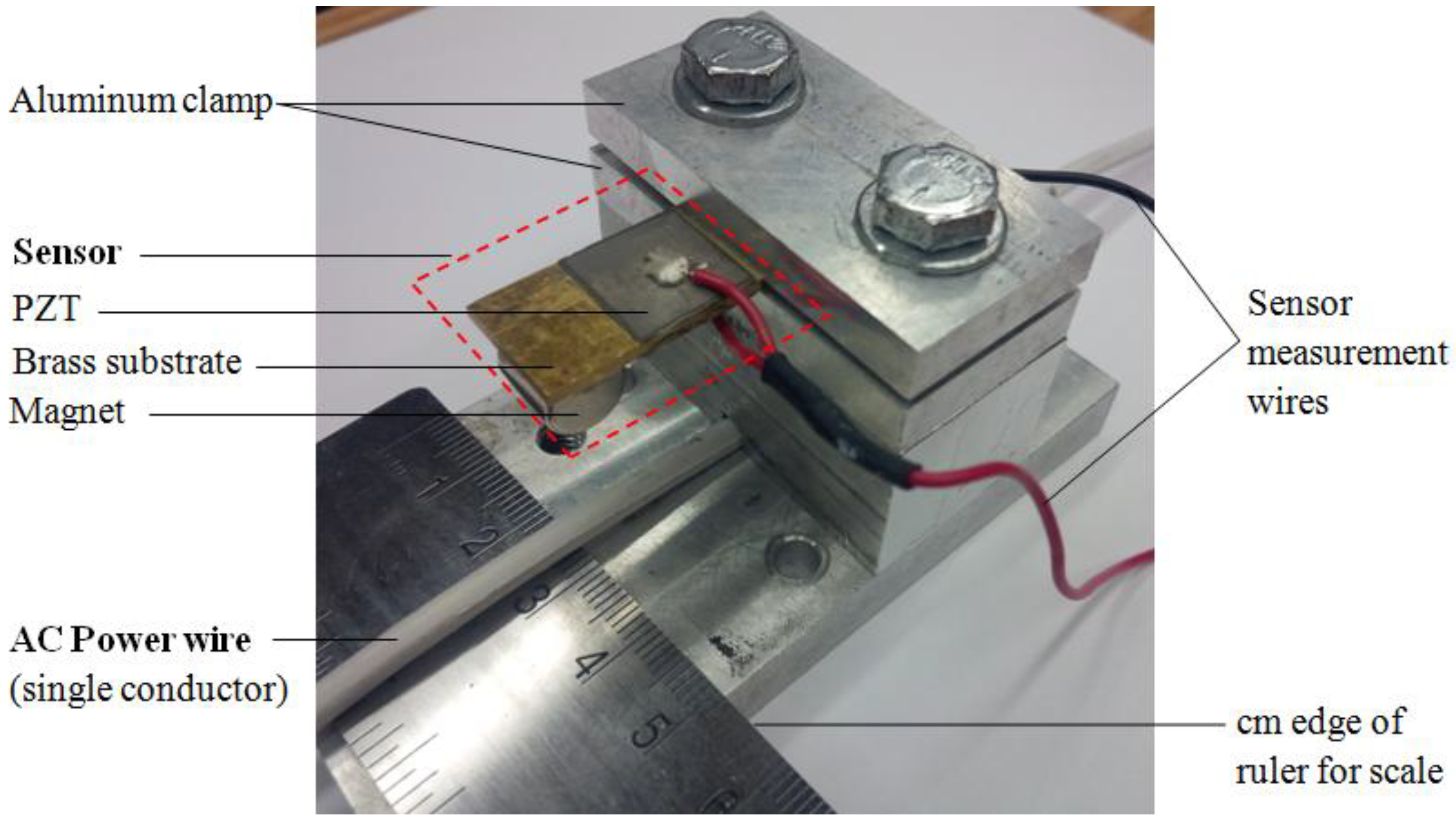
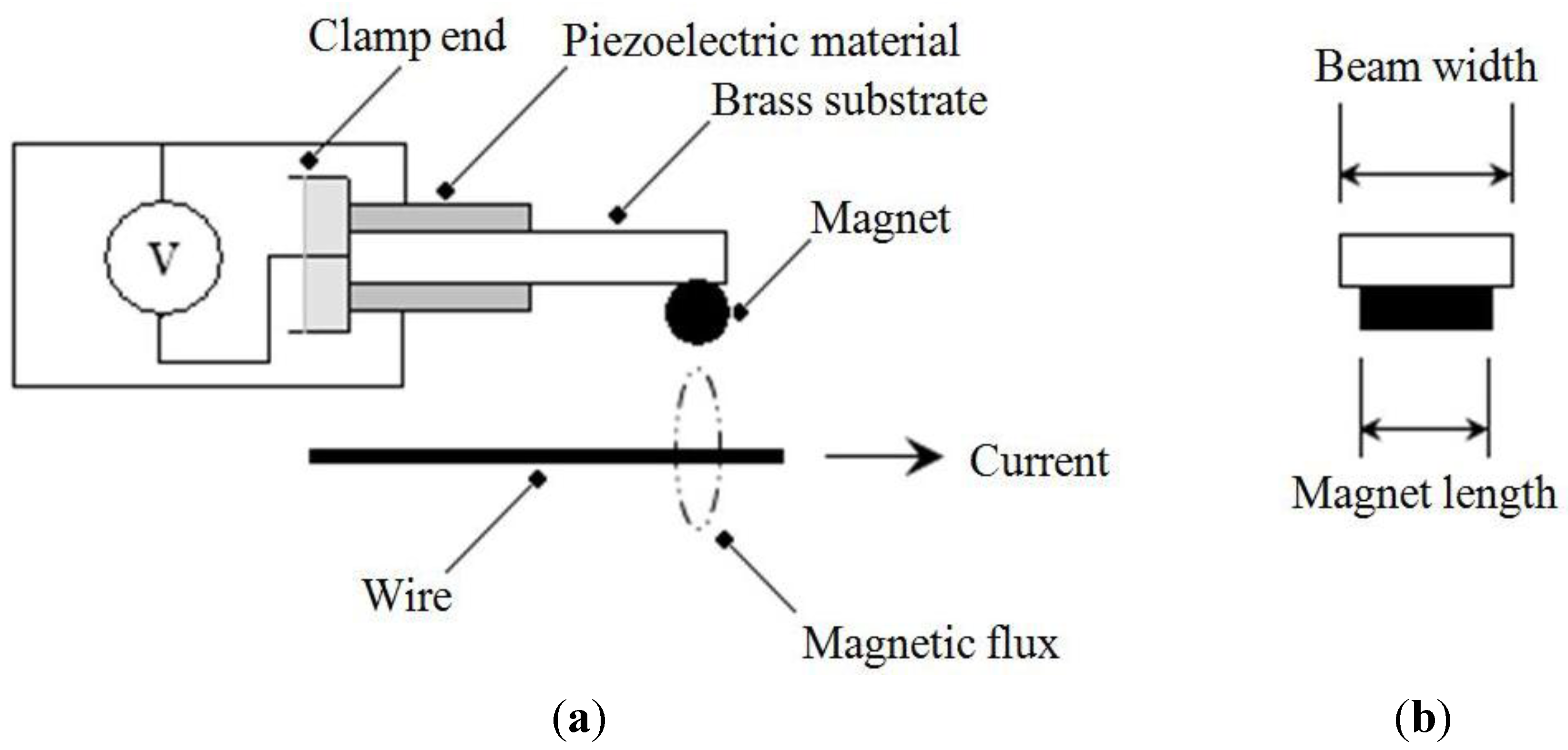
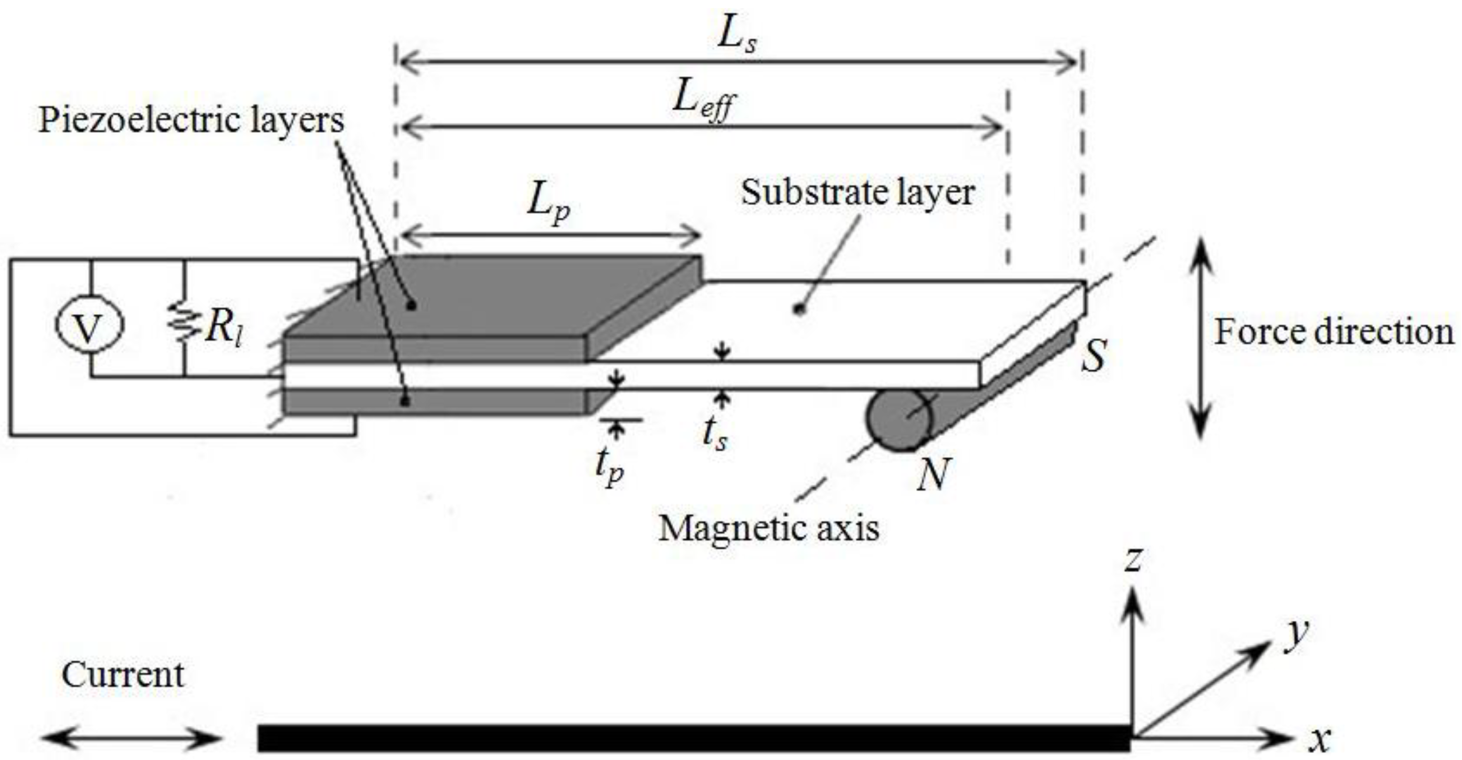
Figure 1.
Schematic of the miniature AC current sensor. (a) Side view; (b) Front view.
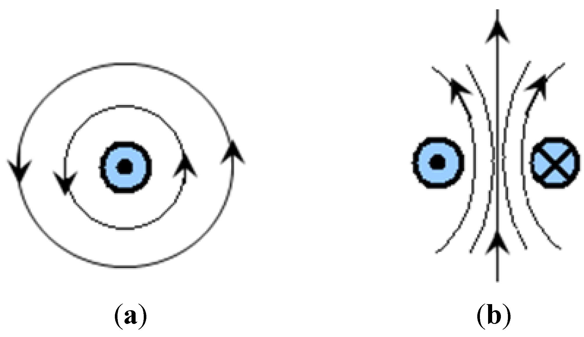
Figure 2.
Magnetic fields of single and double conductors carrying current. (a) Single conductor; (b) Double conductor.
2.1. Electromagnetic Force Modelling
Presented in this section is the derivation for the electromagnetic force on the sensor tip magnet. The interaction between the magnet and the transmission wire can be better understood using Equations (1) and (2). Equation (1) gives the force on a current carrying wire element placed in an external magnetic field [
12].
Here,
I is the current in the wire,
dl is the differential wire element vector (directed along the direction of current flow) and
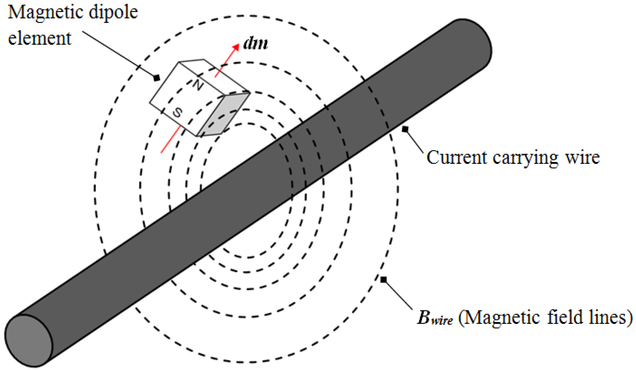
Bmag is the magnetic flux density of the magnetic field produced by the magnet. This force on the wire is equal and opposite to the force on the magnet element. Equation (2) gives the force on a magnetic dipole element placed in an external magnetic field by the wire as illustrated in
Figure 3 [
13].
Here,
dm is the magnetic moment of the magnetic dipole element and
Bwire is the time varying magnetic flux density of the magnetic field produced by the wire.
Figure 3.
Magnetic dipole element placed in the magnetic field of a current carrying wire.
Figure 3.
Magnetic dipole element placed in the magnetic field of a current carrying wire.
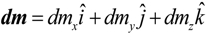
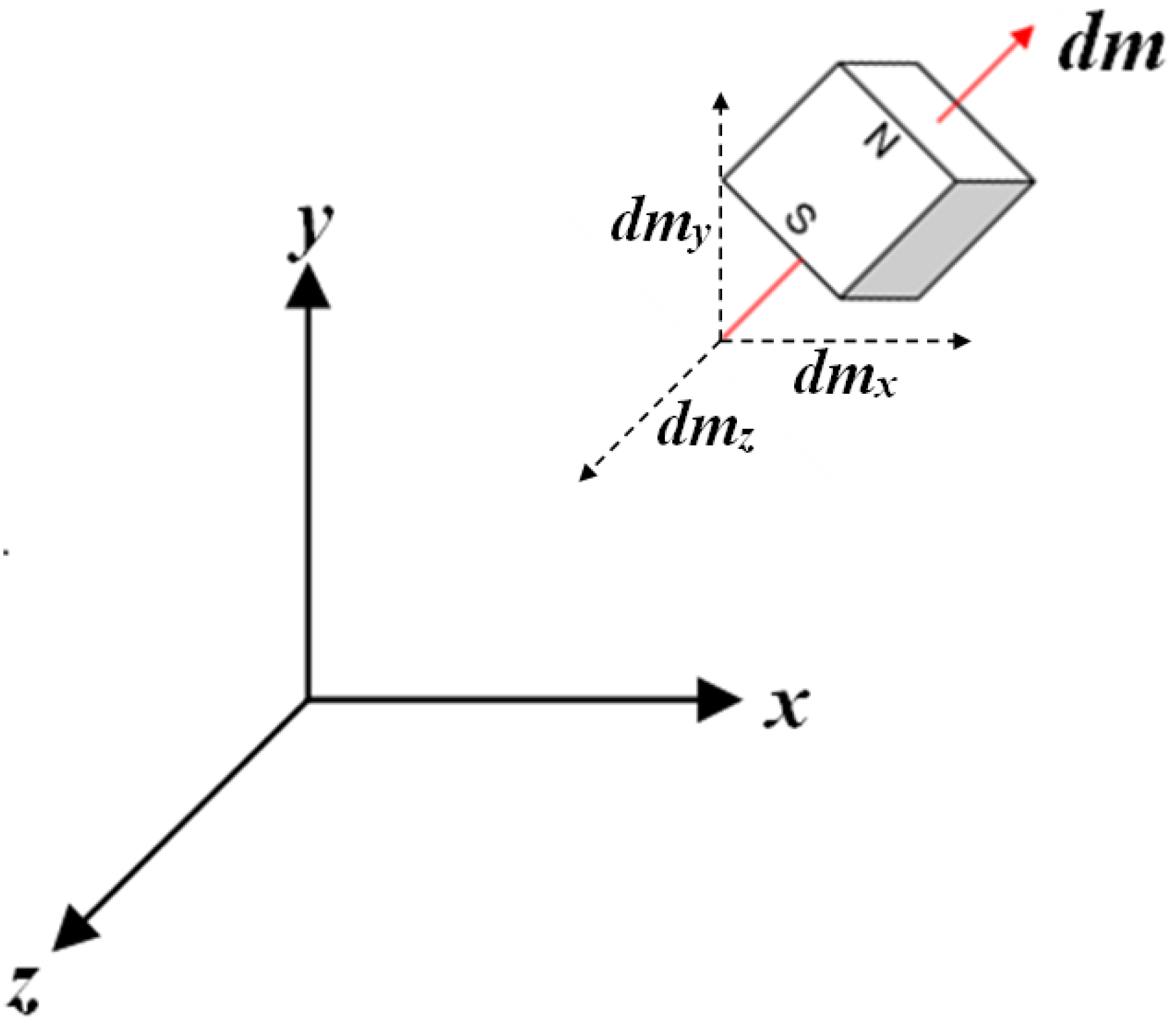
The magnetic moment of the dipole element shown in
Figure 4 can be written as
where
dmx,
dmy, and
dmz are the
x,
y and
z components for any arbitrary orientation of the dipole.
Figure 4.
Magnetic dipole element and the magnetic moment.
Figure 4.
Magnetic dipole element and the magnetic moment.
In addition, the magnitude of the dipole moment can be expressed as
where
Br is residual magnetic flux density or remanence,
dV is the differential volume of the element, and
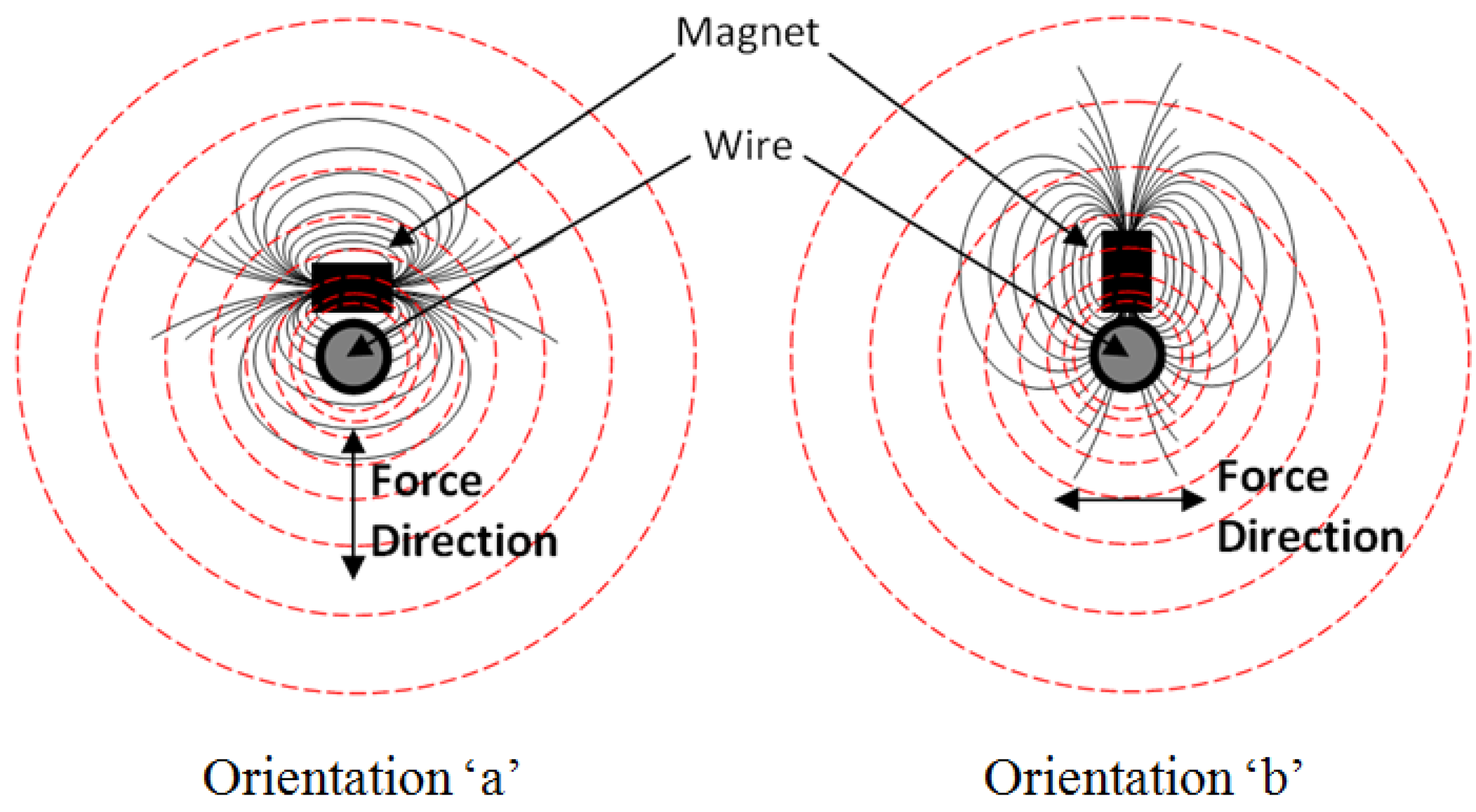
μ is the permeability of air. From Equation (1) it can be seen that, to maximize the force on a current carrying element, it is necessary to maximize the cross product of the external magnetic flux density and the current unit vector. This can be achieved through two different orientations of the magnet.
Figure 5 shows the two orientations that allow the magnetic field lines of a single magnet to be approximately perpendicular to the wire. The dashed lines represent the magnetic field lines of the wire and the solid lines represent the magnetic field lines of the magnet. In orientation “
a”, the magnet is placed such that its magnetic axis is tangent to the lines that represent the magnetic field of the wire. In orientation “
b”, the magnet axis is perpendicular to these lines. Both orientations result in a net force on the wire that is perpendicular to the axis of the magnet. Once again, note that the force on the wire is equal and opposite of the force on the magnet. Intermediate orientations lead to both a reduction in efficiency of the magnetic field interactions, and asymmetric forces, which are undesirable for the sensor design.
Figure 5.
Magnetic fields for “a” and “b” magnet orientations.
Figure 5.
Magnetic fields for “a” and “b” magnet orientations.
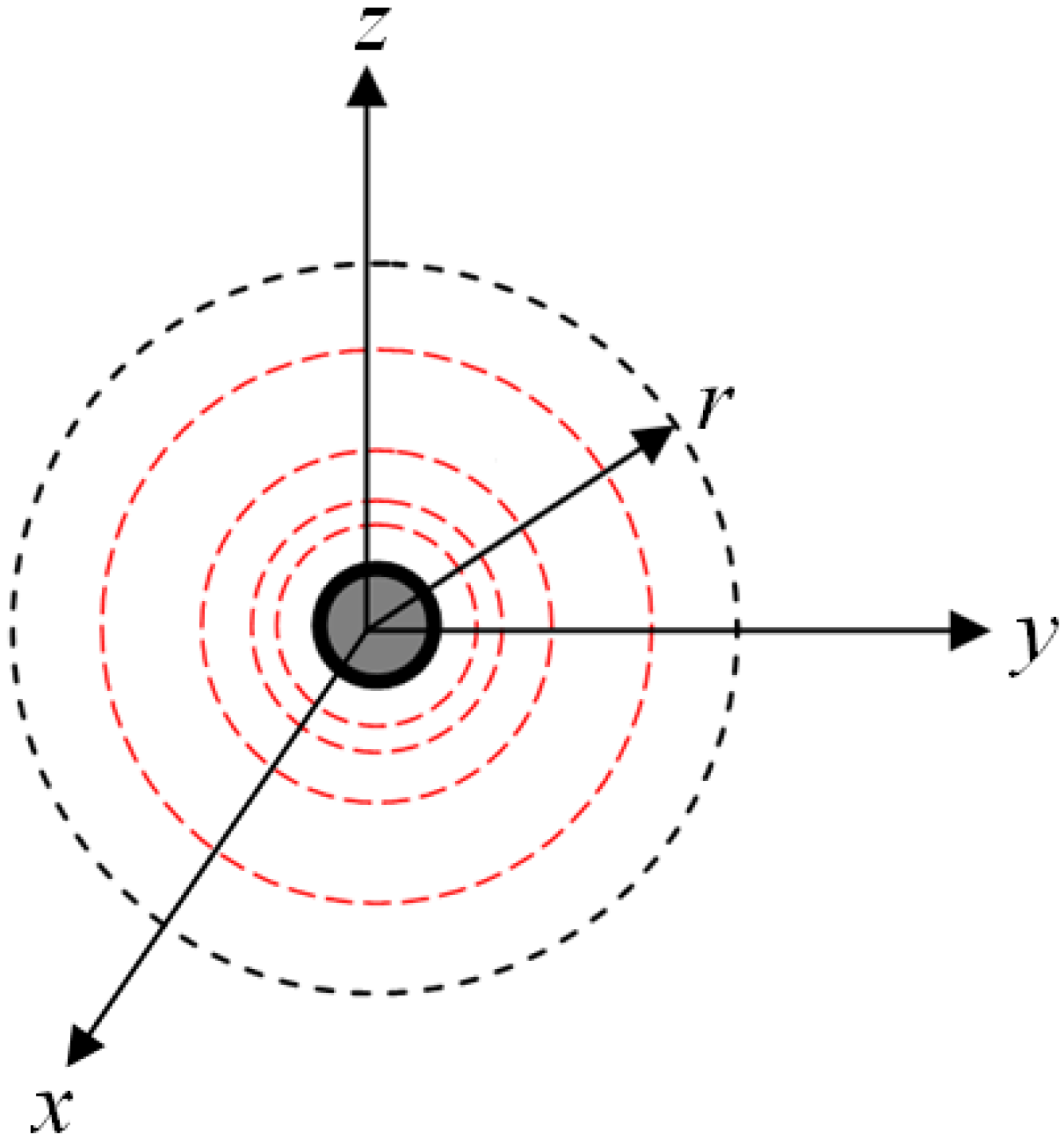
Figure 6.
Coordinate system for a single conductor.
Figure 6.
Coordinate system for a single conductor.
For simplicity, Equation (2) is used instead of Equation (1) to obtain the expressions for the total force on a tip magnet as described below.
Figure 6 shows the coordinate system used for obtaining these expressions. In this figure,
r is the position vector of any point (
y,
z) around the wire (
r =
![Actuators 03 00162 i033]()
). The wire is placed along the
x axis, therefore:
Here Ia is the current amplitude, v is the frequency and t is time.
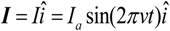
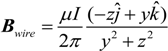
Using Ampere’s law [
12],
the magnetic field around an infinitely long current carrying wire can be expressed as:
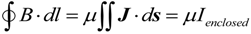
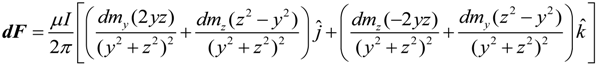
Using the coordinate system show in
Figure 6, Equation (7) simplifies to:
By substituting Equations (3) and (8) in Equation (2), the force on the differential volume of the magnetic element can be found as:
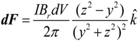
For orientation “
a”, the
j components of the force cancel out due to symmetry. In addition, the magnetic dipole moment along the
i and
k directions is zero. Thus, for this orientation, the following expression for the force on a differential element volume is obtained using Equations (4) and (9):
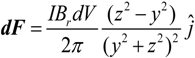
Similarly, the following expression is obtained for orientation “
b”:
The total force on the magnet can then be found by integration over the magnet volume.
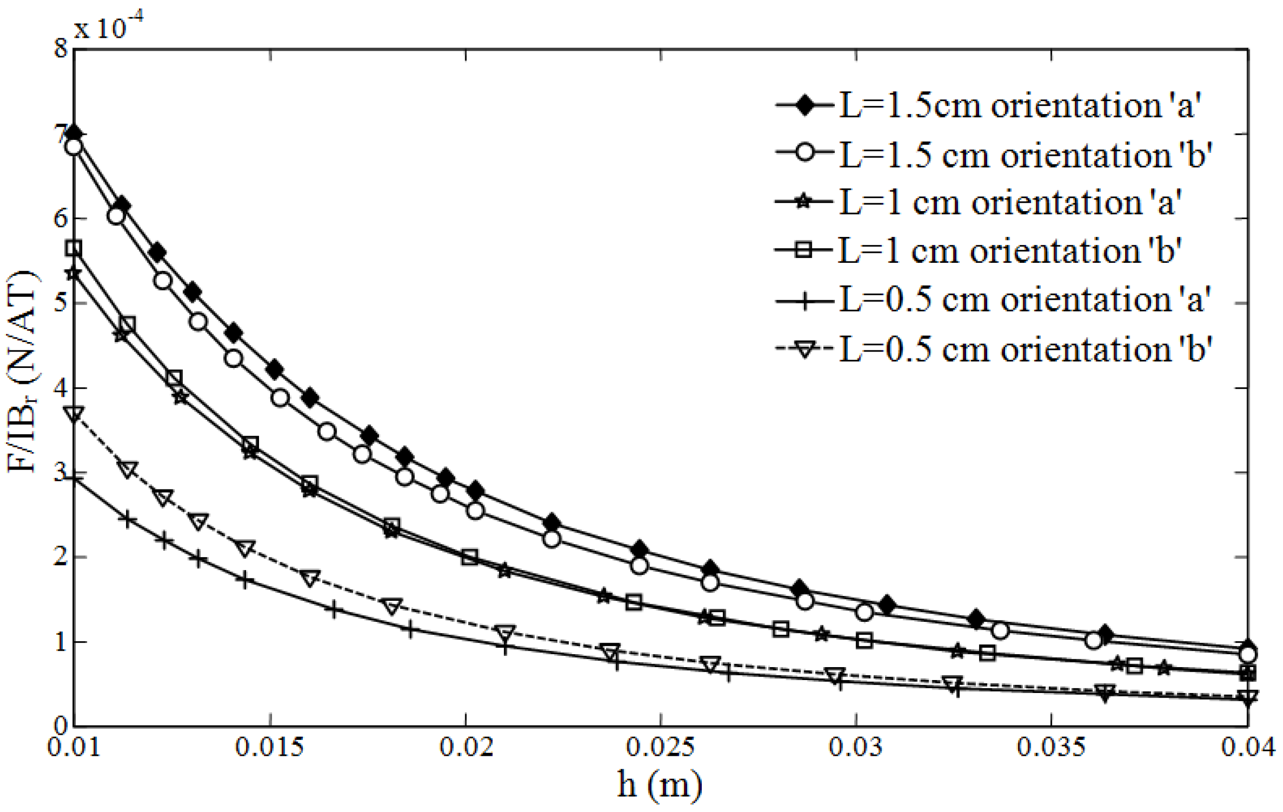
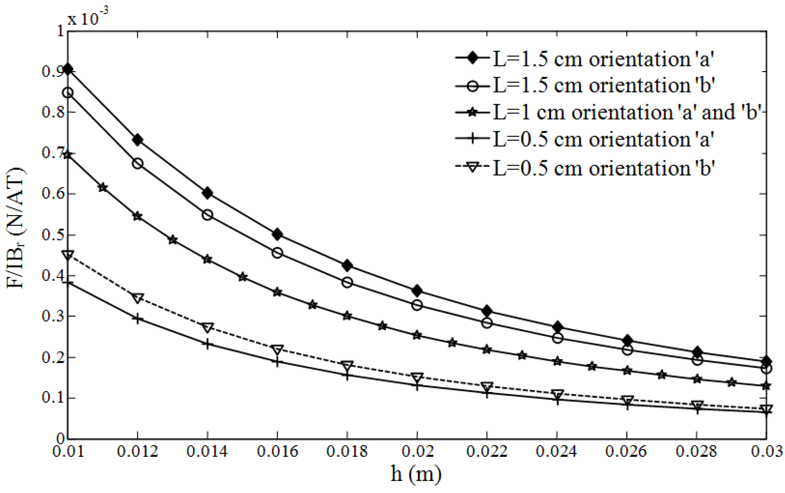
Figure 7 and
Figure 8 present the theoretical force per unit current and unit residual flux density for both orientations “
a” and “
b” for various distances between the wire and the magnet. The results are obtained for both cuboid and cylindrical magnets. Three different magnet lengths of 0.5 cm, 1 cm, and 1.5 cm with a 1 cm
2 cross section are used for both geometries. As illustrated in these figures, the optimal orientation (“
a” or “
b”) depends on the magnet length. For both cuboid and cylindrical geometries, orientation “
a” is shown to produce greater magnetic force values if the length of the magnet is larger than the width (diameter). For lengths equal to the width (diameter) both configurations give similar results.
For the prototype, a cylindrical magnet and orientation “a” were chosen. Orientation “b” is not the most suitable option for a single wire measurement because the force along the magnet varies along its length due to the varying distances of the magnetic elements from the wire. This will result in additional torsional vibrations, which are not desired for the sensor measurement calibration. Additionally, a cylindrical magnet was selected as it allows for a smaller contact area with the beam. This geometry simplifies the dynamic modelling of the sensor since it allows modelling the magnet as a tip mass.
Figure 7.
Theoretical force per unit current and unit residual flux density for cuboid magnets.
Figure 7.
Theoretical force per unit current and unit residual flux density for cuboid magnets.
Figure 8.
Theoretical force per unit current and unit residual flux density for cylindrical magnets.
Figure 8.
Theoretical force per unit current and unit residual flux density for cylindrical magnets.
2.2. Piezoelectric Modelling
The schematic of the proposed model of the sensor is shown in
Figure 9. This sensor configuration allows a more effective forcing mechanism for the sensor compared to Reference [
10] due to the chosen orientation of the magnet with respect to the sensor substrate layer.
A mathematical model is required to predict the sensor output and its dynamic behaviour. The sensor must be designed for the frequency range of interest in such a way that its natural frequency is far from the frequencies of operation. This results in a fairly constant frequency response function (FRF) for the frequency range of interest, which aids in obtaining a non-variable calibration ratio. Additionally, this results in relatively small cantilever deflections for these frequencies as they are far from resonance. Therefore, the deflections are also assumed to have no significant influence on the electromagnetic forces on the tip magnet and this force is assumed to have a harmonic form.
Figure 9.
Schematic of the cantilevered beam sensor.
Figure 9.
Schematic of the cantilevered beam sensor.
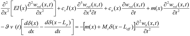
In order to obtain the natural frequency of the sensor, the governing partial differential equation (PDE) for base excitations applied to the clamped end are considered. The theoretical frequency response function for the sensor output voltage to base excitation is later validated through a shaker harmonic testing. The PDE for the sensor depicted in
Figure 9 may be found as follows:
The transverse deflection of the beam relative to the base input excitation at position
x and time
t is
wrel (
x,
t), while the base excitation is denoted by
wb (
x,
t). Note that the total deflection can be found as
wtotal (
t) =
wb (
t) +
wrel (
t). The terms
csI and
ca are the strain rate damping and air damping terms respectively. Air damping is assumed to be negligible in this analysis. The strain rate damping, known as Kelvin-Voight damping, is later incorporated in the modal coordinates through model damping ratios obtained from the experiments [
14].
Leff is the effective length of the beam which is measured from the clamped end to the center of the magnet and
Mt is the total tip mass which includes the magnet, the tip of the beam and the epoxy bonding the two. Finally,
v(t) and
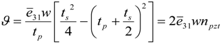
ϑ are the voltage and the electromechanical coupling term for the piezoelectric layers in a parallel configuration respectively. The electromechanical coupling term
ϑ is given by:
Here,
![Actuators 03 00162 i034]()
is a piezoelectric coupling constant,
tp and
ts are the thicknesses of the piezoelectric (one layer) and substrate material, respectively,
w is the width of the beam and
npzt is the distance from the neutral axis of the substrate to the neutral axis of the piezoelectric layer. Equation (12) as a whole is very similar to the expression found in [
14], however, due to the discontinuity in the piezoelectric material, care has been taken to modify the mass per unit length term
m(x) and the bending stiffness term
EI(x) [
15].
2.2.1. Mode Shape Functions
Using mode summations, the response of the system can be described as a series of eigenfunctions (mode shapes) as is commonly done using the separation of variables:
Here,
ϕr (
x) is the mass normalized eigenfunction for an undamped vibration, and
ηr (
t) is the modal mechanical coordinate expression for the
rth vibration mode. However, due to the discontinuity of the piezoelectric layer in the beam, the solution to the spatial ODE is segmented in piecewise sections [
15]:
For piezoelectric-substrate (
Section 1): 0 <
x <
LpFor substrate only (
Section 2):
Lp <
x <
LeffHere constants
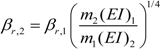
βr,1 and
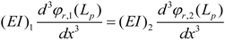
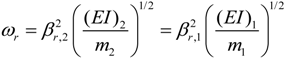
βr,2 are mode shape parameters for each of the two sections. The relation between
βr,1 and
βr,2 may be found as [
15]:
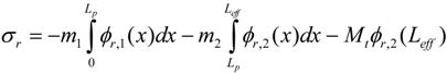
where
m1 and
m2 are the mass per unit lengths for each of the two sections. Also,
(EI)1 and
(EI)2 are the bending stiffness of the two sections.
2.2.2. Boundary Conditions
The boundary conditions and continuity equations that describe the system shown in
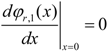
Figure 9 are presented in this section. Equations (18) and (19) are the boundary conditions at the clamped end (
x = 0):
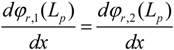
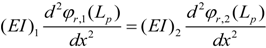
Equations (20) to (23) are the continuity conditions between the two segments of the beam:
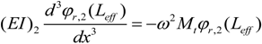
Equations (24) and (25) are the boundary conditions at the free end of the beam (
x =
Leff):
Here,
It and
Mt are the mass moment of inertia and mass of the tip mass. The stated boundary and continuity conditions can be described in the matrix form as follows:
where
Q is a vector of the mode shape coefficients and
P is the multiplier matrix:
For a non-trivial solution, the determinant of
P has to vanish. Using this method, the natural frequencies (short-circuit condition) of the system can then be found as:
2.2.3. Governing Equations of Motion
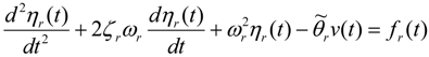
The equations for the modal coordinates can then be determined using Equations (12) and (14) and applying the orthogonality condition as:
where the modal electromechanical coupling term is:
The modal mechanical forcing function for base acceleration is described as:
and the modal mechanical damping ratio
ζr is found using experimental results through the half power method.
2.2.4. Electrical Circuit Equation
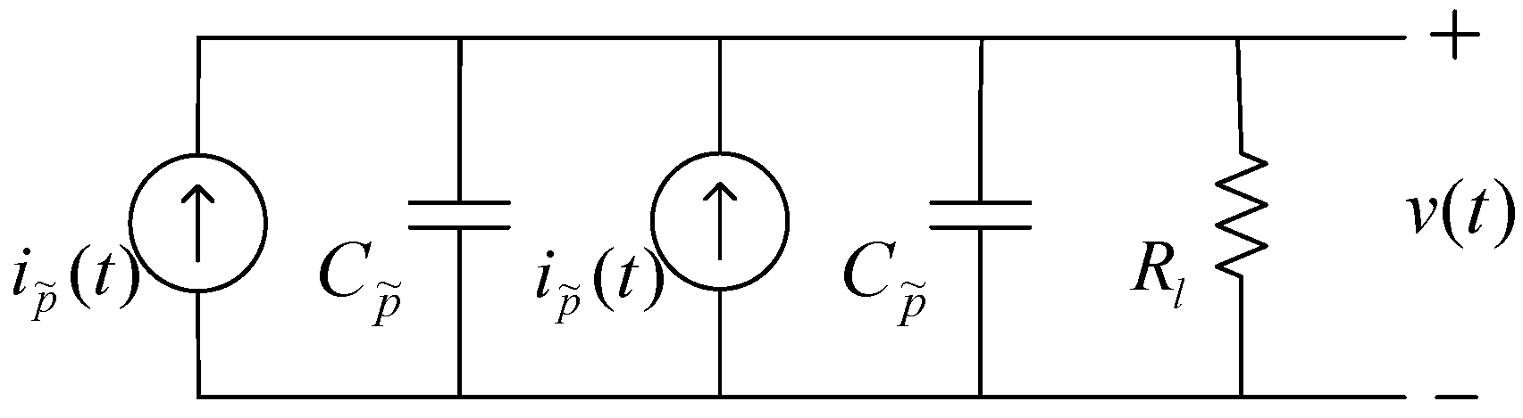
The coupled electrical circuit equation for the bimorph connection in parallel can be derived using Kirchhoff’s law in which the piezoelectric layers are modelled as two current sources in parallel with internal capacitances as shown in
Figure 10 [
14]. The large internal resistance of the measurement unit results in an open circuit condition.
Figure 10.
Piezoelectric sensor circuit representation (parallel circuit connection).
Figure 10.
Piezoelectric sensor circuit representation (parallel circuit connection).
Using Kirchhoff’s law the following equation is formed.
Here,
Rl is the load resistance (measurement unit), and
![Actuators 03 00162 i035]()
is the effective capacitance of both piezoelectric layers. This equation represents the coupled electrical circuit equation used to determine the voltage response of the sensor due to base excitations.
2.2.5. Frequency Response Function and Forcing Functions
Assuming harmonic functions,
i.
e.,
ηr(
t) =
Hrejωt and
v(
t) =
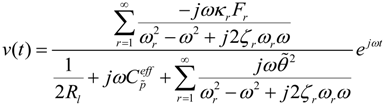
Vejωt, the steady state modal mechanical response of the beam and steady state voltage response across the resistive load, Equations (29) and (32) become:
By substitution of Equations (33) and (34), one can obtain the open circuit natural frequency and steady-state voltage response as [
14]:
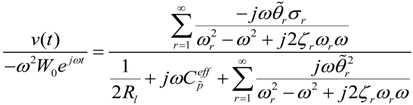
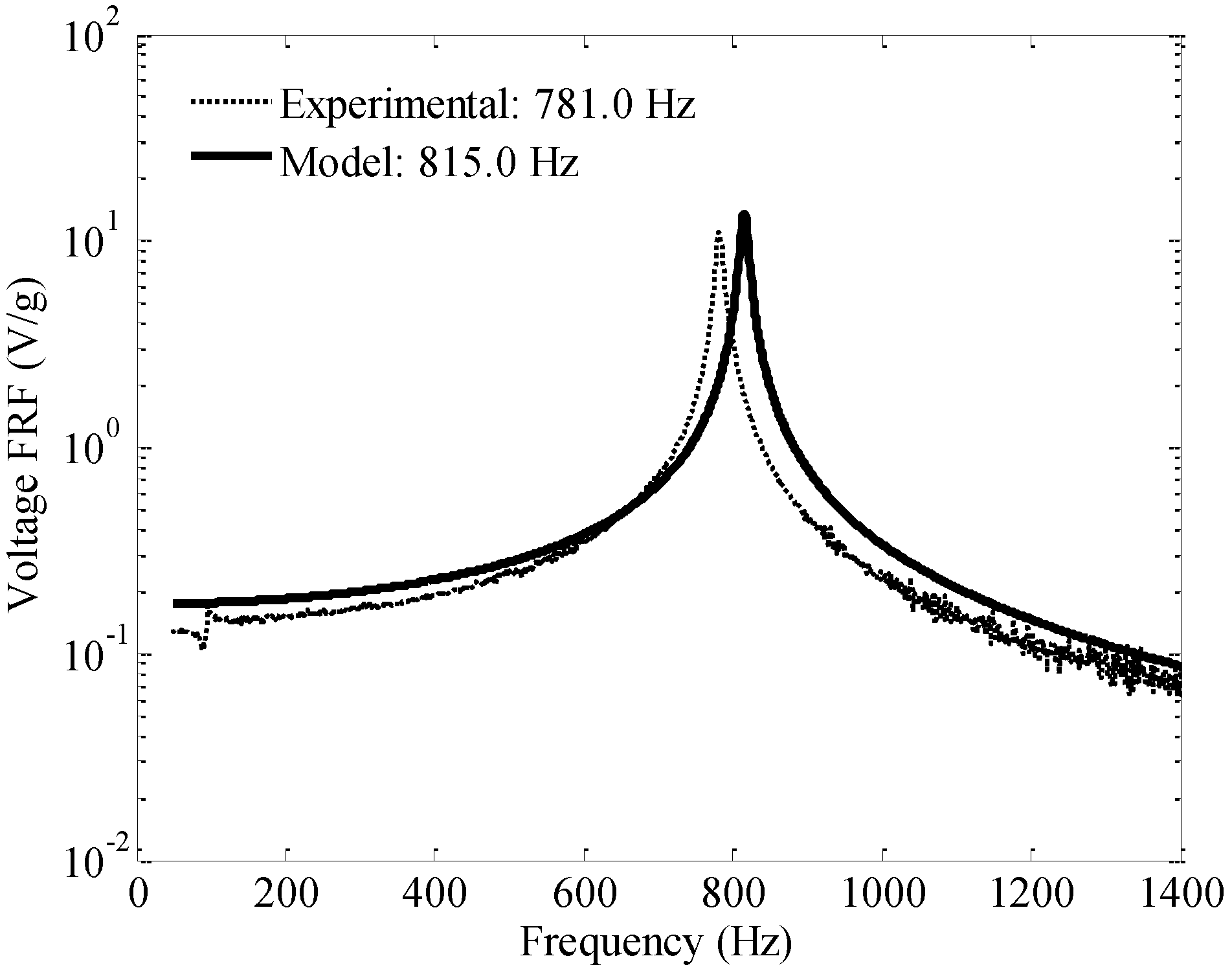
The voltage output to base acceleration FRF can then be found as:
where
Fr = −
σrω2Wo defines the base acceleration forcing function,
σr defines the forcing function as:
and
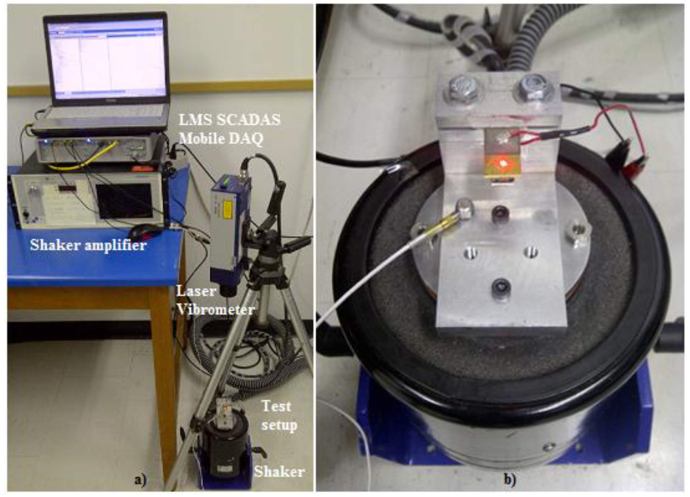
W0 is the base displacement amplitude. The FRF found using this method can then be validated through testing by mounting the sensor on a shaker that provides base acceleration in order to produce the voltage output in the piezoelectric layers. The analytical and experimental test results are compared and discussed later in
Section 3 of this paper.
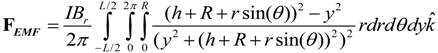
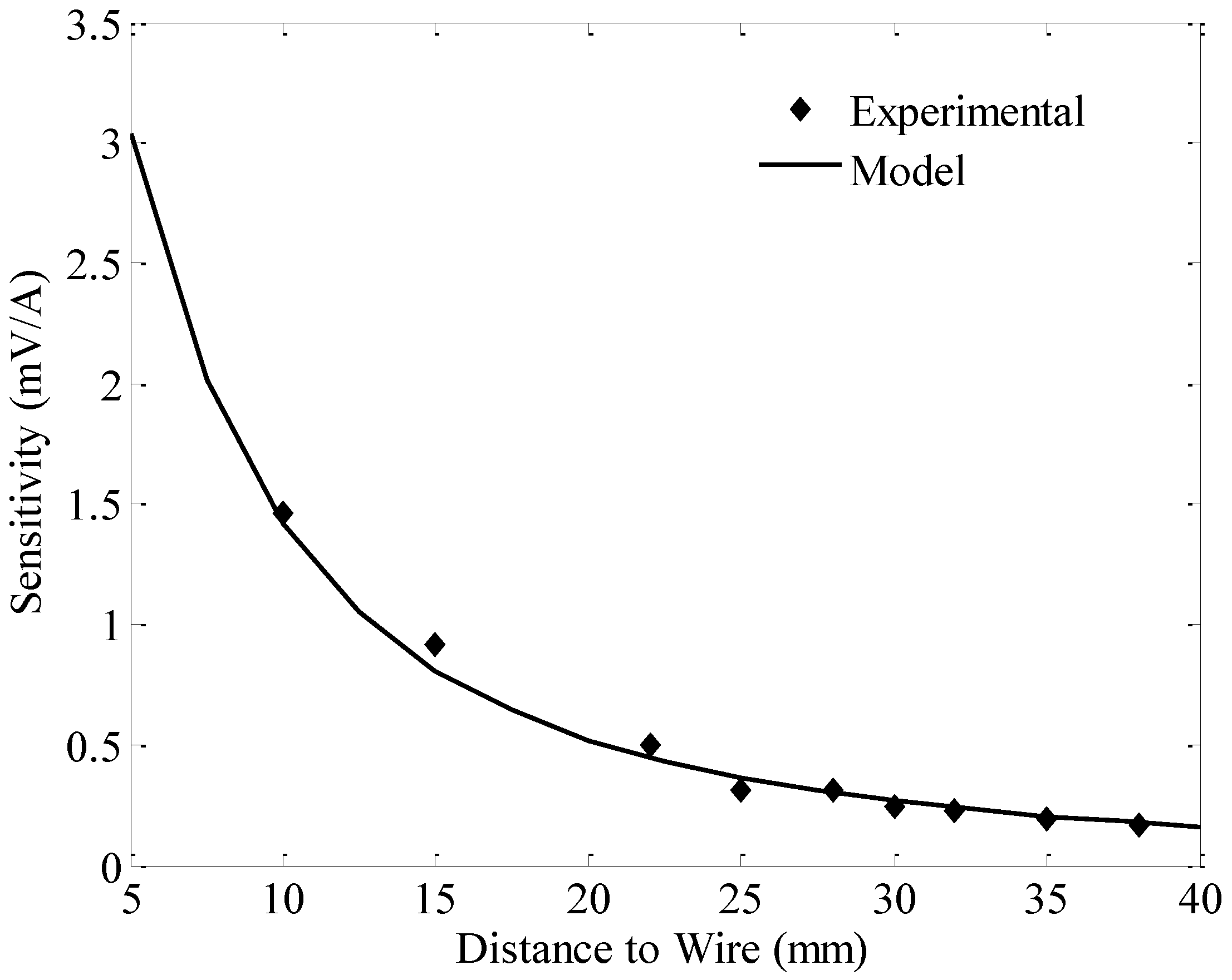
The second part of this modelling focuses on obtaining the sensor sensitivity which is defined as the sensor output voltage per input current passing through a wire in the proximity of the sensor. As discussed previously, the input current results in an electromagnetic force on the tip magnet. This force can be obtained by integrating Equation (10) over the volume of the cylindrical magnet shown in
Figure 9 as follows:
Here, h is the distance from the center of the wire to the closest point of the magnet, the length of the magnet L is measured along the magnetic axis and R is the radius of the magnet. This relation is then used to obtain the output voltage for the sensor when placed at the proximity of a current carrying wire.
2.2.6. Design Considerations
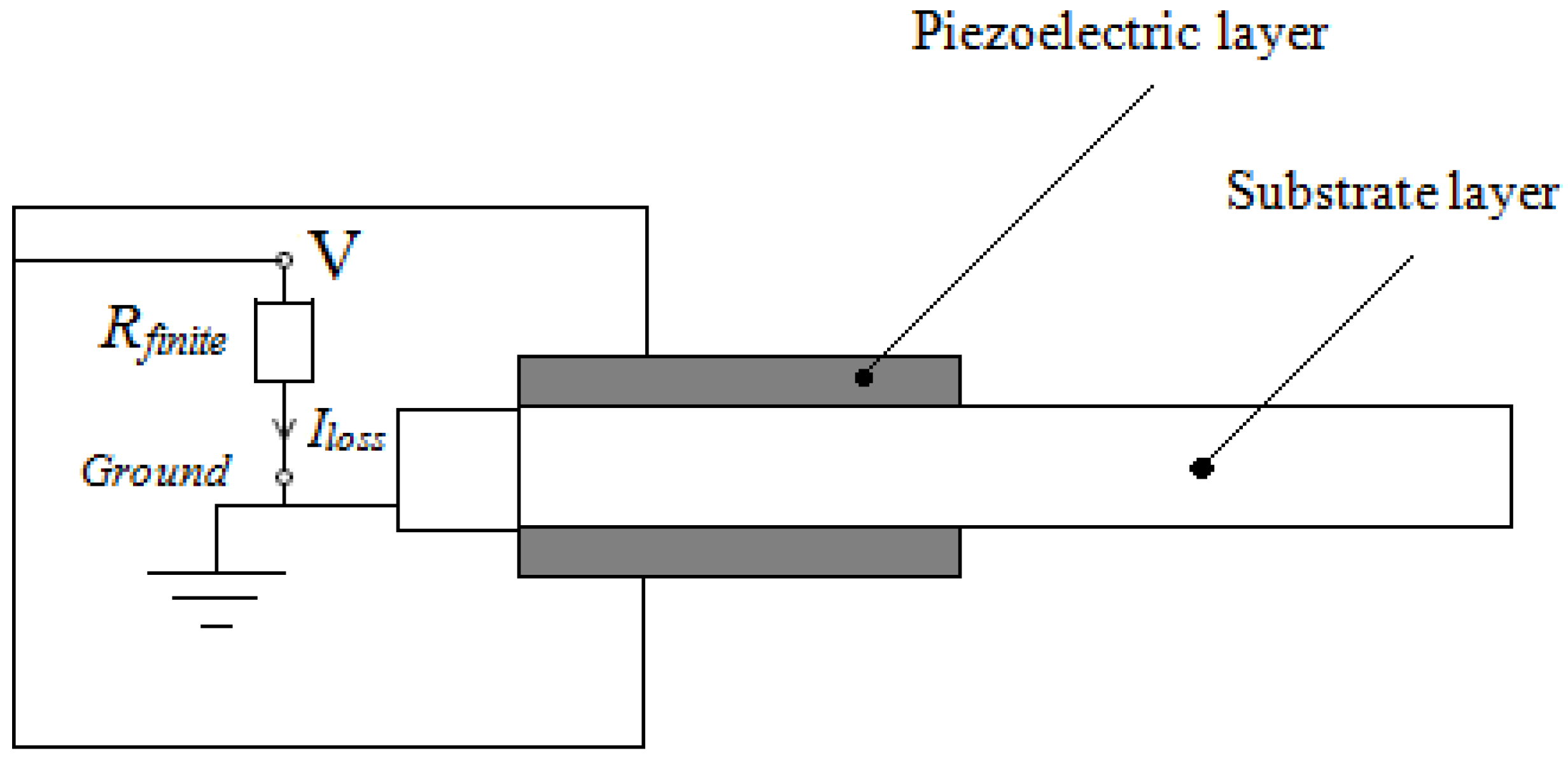
2.2.6.1. Voltage Loss
If a voltage measurement unit with finite inner resistance is connected to the contacts of the piezoelectric sensor, a current
Iloss will flow and, thus, the charge displacement on the piezoelectric electrodes will change.
Figure 11 shows this equivalent circuit and the current loss schematic.
Figure 11.
Equivalent circuit and the current leakage.
Figure 11.
Equivalent circuit and the current leakage.
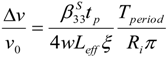
This change in charge displacement will result in a voltage loss across the piezoelectric layers, which is not desirable for a sensing application. Using Ohm’s law and the constitutive equations for a piezoelectric bimorph, the following equation may be found for the relative voltage-loss in a quarter period of the oscillating voltage across the piezoelectric layers.
Here,
v0 is the amplitude of the output voltage,
Tperiod is the period of the sinusoidal function,
Ri is the inner resistance of the voltage measurement unit, which is assumed to be 100 times the impedance of the sensor (see
Section 2.2.6.2), andis the dielectric permittivity at constant strain. A value of approximately 2.36% was obtained for this ratio for the sensor after parameter optimization, which is acceptable for the design criteria. In addition, gravity effects, temperature expansion or an offset of the input signal may all produce a static offset for the sensor measurements. However, this is not a concern for an AC current sensor since the offset will be in the form of a static signal and will decay after a short period of time.
2.2.6.2. Sensor Impedance
As shown by Staines
et al. [
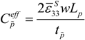
16], and also demonstrated in Equations (39) and (40), the voltage loss through the sensor is inversely proportional to the capacitance of the sensor. Note that the sensor capacitance is also inversely proportional to its impedance. Hence, generally, the sensor must be designed in a way that its impedance is low (high capacitance) compared to the inner resistance of the measurement device in order to reduce the measurement noise level. A ratio of 100 was considered between the impedance of the sensor and the voltage measurement unit to be used during the sensor’s actual operation. On the other hand, the sensor must be designed to guarantee an operation mode close to an open circuit condition, which ultimately requires a large impedance. The sensor capacitance under unstrained condition is defined as:
Here,
![Actuators 03 00162 i037]()
is the dielectric permittivity of the piezoelectric material. The factor of two appears because the sensor is configured in parallel mode. The sensor impedance was found to be about 55 kΩ.
2.2.6.3. Electromagnetic Loss
The substrate material is a nonmagnetic material and is used in commercially available bimorph sensors and actuators. In addition, the induced eddy currents due to vibration of the substrate and the variable magnetic field are assumed negligible in this research. These eddy currents will result in additional damping and power loss by the substrate that can be approximated by [
17]:
where
Ploss is the total power dissipation,
Bp is the peak flux density,
f is the frequency at which magnetic flux density changes, and
ρs is the resistivity of the substrate. Therefore, due to the relatively high resistivity of the brass substrate and its small thickness, the power loss due to the eddy current effects is ignored.
2.2.6.4. Final Design Parameters
The design specifications and constraints considered for this sensor are shown below in
Table 1.
Table 1.
Design specifications and constraints considered for the sensor design.
Table 1.
Design specifications and constraints considered for the sensor design.
| Specification | Value/Range |
|---|
| Sensor operating current range | 10 A–200 A |
| Sensor accuracy within | 1% @ 10–100 A, 4% @ 100–200 A |
| Operating temperature | −40 °C to 80 °C |
| Output voltage for 10,000 A | ±1.75 V |
| Sensor impedance | 55 kΩ |
The internal impedance of the sensor was chosen to be small compared to the voltmeter circuit inner impedance in order to reduce the measurement noise level as explained previously. Based on the design constraints, the values shown in
Table 2 were obtained and selected for the sensor dimensions and other parameters. A D66SH (K&J Magnetics) magnet and the PZT-5A piezoelectric material were selected as they were the most suitable for the wide range of design temperatures. In particular, PZT-5A has a high sensitivity and very good temperature stability over the operating range of temperatures and is commonly used for commercially available sensors and actuators [
18].
Table 2.
Sensor Parameters.
Table 2.
Sensor Parameters.
| Property | Value/Type |
|---|
| Substrate material | Brass 260 (McMaster Carr) |
| Ls | 26 mm |
| ts | 1.55 mm |
| w | 14.45 mm |
| Leff | 20.5 mm |
| Piezoelectric material | PZT-5A4E (Piezo Systems, Inc.) |
| ξ | 0.75 |
| Lp | ξ · Leff (mm) |
| tp | 0.127 mm (each layer) |
| Magnet | D66SH (K&J Magnetics) |
| Rl | 1 MΩ (Measurement Device Resistance) |


 ). The wire is placed along the x axis, therefore:


 is a piezoelectric coupling constant, tp and ts are the thicknesses of the piezoelectric (one layer) and substrate material, respectively, w is the width of the beam and npzt is the distance from the neutral axis of the substrate to the neutral axis of the piezoelectric layer. Equation (12) as a whole is very similar to the expression found in [14], however, due to the discontinuity in the piezoelectric material, care has been taken to modify the mass per unit length term m(x) and the bending stiffness term EI(x) [15].
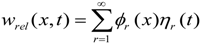


 is the effective capacitance of both piezoelectric layers. This equation represents the coupled electrical circuit equation used to determine the voltage response of the sensor due to base excitations.
 is the dielectric permittivity of the piezoelectric material. The factor of two appears because the sensor is configured in parallel mode. The sensor impedance was found to be about 55 kΩ.
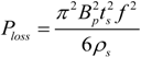
