Article

Fault Diagnosis in Robot Drive Systems Using Data-Driven Dynamics Learning

Department of Electrical Engineering, Pohang University of Science and Technology, 77 Cheongam-ro, Nam-gu, Pohang 37673, Republic of Korea
Actuators 2025, 14(12), 583; https://doi.org/10.3390/act14120583 (registering DOI)
Submission received: 1 October 2025 / Revised: 14 November 2025 / Accepted: 23 November 2025 / Published: 2 December 2025
(This article belongs to the Special Issue Actuation and Sensing of Intelligent Soft Robots)

Abstract

Reliable fault diagnosis in industrial robots is essential for minimizing downtime and ensuring safe operations. Conventional model-based methods often require detailed system knowledge and struggle with unmodeled dynamics, while purely data-driven approaches can achieve good accuracy but may not fully exploit the underlying structure of robot motion. In this study, we propose a feature-informed machine learning framework for fault detection in robotic manipulators. A multi-layer perceptron (MLP) is trained to estimate robot dynamics from joint states, and SHapley Additive exPlanations (SHAP) values are computed to derive discriminative feature representations. These attribution patterns, or SHAP fingerprints, serve as enhanced descriptors that enable reliable classification between normal and faulty operating conditions. Experiments were conducted using real-world data collected from industrial robots, covering both motor brake faults and reducer anomalies. The proposed SHAP-informed framework achieved nearly perfect classification performance (0.998 ± 0.003), significantly outperforming baseline classifiers that relied only on raw kinematic features (0.925 ± 0.002). Moreover, the SHAP-derived representations revealed fault-consistent patterns, such as enhanced velocity contributions under frictional effects and joint-specific shifts for reducer faults. The results demonstrate that the proposed method provides high diagnostic accuracy and robust generalization, making it well suited for safety-critical applications and predictive maintenance in industrial robotics.

1. Introduction

Modern manufacturing heavily relies on industrial robots that deliver consistent precision and productivity [1,2,3,4,5]. As factories become increasingly automated, ensuring long-term operational stability has become just as important as speed and accuracy [6,7]. Nevertheless, degradation of mechanical parts such as gears, reducers, and brakes often leads to subtle yet problematic failures that are difficult to detect at an early stage [8].
Classical fault detection techniques, which rely on mathematical models or observer-based schemes [9,10,11,12,13], require accurate parameter identification and detailed system knowledge, making them sensitive to varying operating conditions and environments. In contrast, purely data-driven algorithms [14,15,16,17] offer greater flexibility but often act as black boxes, limiting their trustworthiness in safety-critical applications. Recent advances in data-driven approaches have introduced a variety of architectures with distinct strengths. Convolutional neural networks (CNNs) are effective at capturing spatial correlations but require extensive data and lack physical interpretability. Recurrent and long short-term memory (RNN/LSTM) networks can model temporal dependencies in sequential data but are computationally intensive and prone to vanishing gradients. Transformers address long-range dependencies through attention mechanisms, yet they often demand large-scale datasets and heavy computational resources. In comparison, the multilayer perceptron (MLP) provides a lightweight feedforward architecture that can approximate nonlinear relationships with relatively low computational cost. Although MLPs may not explicitly capture temporal context, they are well suited for structured input features, such as windowed torque and current time-series signals. To leverage the advantages of both approaches, recent research has focused on physics-informed data-driven approaches [18,19,20,21,22] that integrate physical modeling with learning-based adaptability, providing a balance between interpretability and generalization, as conceptually illustrated in Figure 1.
Explainable artificial intelligence (XAI) has been introduced as a promising solution to enhance the transparency of machine learning models, such as SHapley Additive exPlanations (SHAP), Local Interpretable Model-agnostic Explanation (LIME), and Integrated Gradients [23,24,25]. These works highlight complementary advantages and trade-offs among XAI methods—SHAP providing high attribution consistency, LIME offering intuitive local explanations, and Integrated Gradients capturing gradient-based sensitivity. Among them, SHAP has gained attention for attributing a model’s output back to its input features using cooperative game theory [26]. SHAP has the ability to generate consistent and interpretable feature attributions across complex datasets such as a robot’s joint states. While it has already shown promise in diverse fields, its use remains in robotics relatively recently [27,28,29,30], particularly for uncovering how hidden states of neural models reflect physical fault mechanisms. Including such comparative perspectives strengthens the rationale that SHAP-based fingerprints constitute a useful contribution in physics-informed diagnosis for industrial robots.
In this study, we propose a SHAP-informed fault diagnosis framework for industrial robots that leverages measured joint states (positions, velocities, and accelerations) and torque signals. Unlike conventional classifiers that directly map raw sensor data to fault labels, our method first learns the underlying robot physics—capturing both conservative and non-conservative forces such as friction—from the data. SHAP analysis is then applied to this learned model to derive discriminative feature representations, which enhance the separation between normal and faulty operating conditions. Experimental validation on real industrial robots with both brake and reducer faults demonstrates that the proposed method achieves improved classification performance compared to baseline MLP classifiers, while also revealing fault-consistent patterns that improve robustness and diagnostic reliability.

2. Methodology

2.1. Robot Dynamics and MLP-Based Learning

The dynamics of an n-DoF industrial robot can be expressed by the standard rigid-body formulation:
τ model = M ( q ) q ¨ + C ( q , q ˙ ) q ˙ + g ( q )
where q , q ˙ , q ¨ are joint positions, velocities, and accelerations; M is the inertia matrix; C represents Coriolis and centrifugal effects; and g denotes gravitational torques. In practice, deriving M , C , and g precisely for complex robotic manipulators is challenging. These parameters are typically defined using industrial robot analysis tools in field applications, from which analytical torque predictions can be obtained. However, unmodeled dynamics τ u n m o d e l (e.g., frictional losses, gear reducer wear) often introduce discrepancies between the measured torques τ measured and the analytical predictions τ model . To address this, we define the unmodeled torque τ unmodel :
τ unmodel = τ fric + τ err + η ( t )
τ measured = τ model + τ unmodel = τ model + τ fric + τ err + η ( t )
τ fric ( q ˙ ) = F c · sgn ( q ˙ ) + F v · q ˙ + F s F c · e | q ˙ | v s 2 · sgn ( q ˙ ) ,
where τ unmodel denotes the sum of the generalized friction torque, τ fric , and the model error, τ err , following classical physical laws [31,32,33], and η ( t ) represents additional sensor measurement noise and bias, which can be significant at high sampling rates and may affect feature attribution in learning-based models. In Equation (4), F c represents the Coulomb friction that remains constant in magnitude but reverses direction depending on the velocity sign, F v denotes the viscous friction that increases linearly with velocity, and the exponential term models the Stribeck effect, following classical Dahl and Karnopp descriptions [32,33], where the static friction F s gradually decreases to the Coulomb friction level F c as the velocity increases, with v s controlling the transition rate. While these classical friction models capture essential physical effects, they are approximations and may break down under certain conditions, such as temperature dependence, lubricated contacts, or stick–slip phenomena at very low velocities. The friction parameters F s , F c , F v , and v s were estimated individually for each joint. We confirmed that site-to-site variations or misspecifications of these friction constants did not lead to a degradation of the overall manipulator performance. Across a variety of robot inspection cases, such parameter deviations did not affect the diagnostic results, as the proposed method relies on the attribution of measured joint variables to output torque rather than on the absolute values of the friction constants. Moreover, preprocessing and the MLP are assumed to partially mitigate the effects of these uncertainties.
In classical mechanics, conservative forces are those derived from a potential function, such as gravity or elastic forces, and their energy is preserved in the system. In contrast, non-conservative forces do not admit a potential function and are associated with energy dissipation or anomalies, such as friction, backlash, or potential faults in the drive system. Therefore, the measured torque τ measure encodes both conservative forces, which are preserved in the kinematic structure of the manipulator defined by the Denavit–Hartenberg (DH) parameters [34], and non-conservative forces that reflect frictional effects and possible system faults.
To capture the nonlinear structure of τ measure , we employ an MLP f ( x ) with joint states x = [ q , q ˙ , q ¨ ] as input and τ measure as output:
τ measure f ( x ) ,
where the MLP is trained using mean squared error (MSE) loss:
L = 1 N i = 1 N τ measure ( i ) f ( x ( i ) ) 2 .
In practice, the loss function also incorporates normalization terms based on the variances of joint variables and torque, and an additional energy-consistency term to enforce the physical constraint H ˙ pred H ˙ . These normalization and energy-consistency terms acted as implicit regularization, constraining the learned dynamics within physically plausible ranges. This dynamics learning framework allows the network to encode effects that are difficult to model explicitly, such as joint friction, backlash, and reducer wear. Importantly, the learned representation captures how faults alter the relationship between motion states and torque, providing discriminative patterns that enhance fault diagnosis. The overall workflow of the proposed method is shown in Figure 2.

2.2. SHAP-Based Attribution Analysis

To interpret how each input feature contributes to τ measure , we apply SHAP to the trained MLP. SHAP decomposes the model output into additive feature attributions:
f ϕ ( x ) = ϕ 0 + i = 1 d ϕ i ,
where ϕ 0 is the baseline output and ϕ i quantifies the marginal contribution of feature x i .
In this study, SHAP values are computed using a model-agnostic KernelSHAP algorithm suitable for general black-box models. To preserve the structural information of the learned latent features, feature contributions are estimated on the hidden-layer representation of the trained dynamics MLP. Specifically, the hidden-layer activations are obtained via an extraction function, which extracts the output of intermediate layers given the concatenated input matrix X R N × 24 consisting of joint positions (q), velocities ( q ˙ ), accelerations ( q ¨ ), and joint torques ( τ ).
Since x is composed of joint positions, velocities, and accelerations, SHAP values provide a feature-wise importance map that highlights whether torque terms are primarily influenced by q ˙ or q ¨ . According to the friction model in Equation (4), friction is associated with static and dynamic components, where the dynamic component is directly related to q ˙ . In contrast, q ¨ does not appear explicitly in the friction equation; rather, as shown in the dynamics formulation in Equation (1), it is mainly involved in model compensation. Therefore, q ˙ can be regarded as capturing friction-related effects, while q ¨ reflects model compensation. By aggregating SHAP values across input groups, we obtain joint-wise fingerprints:
Φ j = i G j | ϕ i | , j = 1 , , n ,
where G j indexes the input features associated with joint j.

2.3. Fault Classification Framework

The joint-wise SHAP fingerprints Φ j are then used to train a binary classifier that distinguishes between normal and faulty conditions. Each sample’s SHAP tensor is flattened into a feature vector and passed through an MLP-based classifier. This approach offers two benefits: (1) accurate classification of fault vs. normal samples, and (2) feature-informed representations that highlight which joints and input features are most strongly associated with fault signatures. As a result, the framework enhances diagnostic reliability by combining data-driven fault detection with physically consistent feature patterns.

3. Experimental Setup

3.1. Robot Platform and Fault Conditions

The experimental platform consists of a six-degree-of-freedom (6-DoF) articulated industrial manipulator equipped with rotary joints driven by servo motors and Rotary Vector (RV) reducers, as shown in Figure 3. The manipulator has a rated payload capacity of 165 kg, making it representative of heavy-duty robots frequently deployed in welding and material-handling tasks. For one fault case, Figure 4 depicts the real robot used in the production process, showing wear of the reducer and deformed gear tooth profiles caused by insufficient grease lubrication.
Each servo motor comprises the essential components of a typical electromechanical actuator, including a coil, permanent magnet, gear, and shaft. In addition, an electromagnetic brake is integrated, which is constructed from a friction disk, armature plate, coil, and spring, ensuring the motor can safely hold position when power is removed. The brake operates on a fail-safe principle: when power is applied, the electromagnetic field attracts the armature plate and separates it from the friction disk, allowing free rotation of the shaft. When power is removed, the magnetic field disappears and the spring force presses the armature plate against the friction disk, thereby locking the shaft in place.
The drive system further incorporates RV reducers, whose structure consists of gears, bearings, and supporting elements designed to transmit high torque with minimal backlash. The primary purpose of using RV reducers is to increase output torque while reducing motor speed, thereby enabling precise and stable motion control of the robot joints. Their operation relies on a two-stage reduction mechanism, where a cycloidal gear engages with needle bearings and output gears, effectively distributing the load across multiple contact points to achieve high efficiency, durability, and low backlash. Two representative fault categories were investigated in this study: reducer-related degradation and brake-related anomalies.
  • Motor brake fault: A degradation in the braking mechanism, resulting in increased dynamic friction and resistance during commanded motions. This fault typically manifests as higher torque demand and irregular stopping performance. The nominal performance of the brake is specified as follows: a static friction torque of at least 8.0 Nm, an input power of 12.8 W at 20 °C, and a rotational inertia of 0.45 × 10 4 kg·m2. Brake faults can manifest electrically through anomalies in the release or pull-in voltages. In the present experiments, only the fully engaged (severe) fault state was tested. Degradation mechanisms include a reduction in spring tension, defects in the coil (electromagnet), or insufficient power margin, all of which can compromise braking performance.
  • Reducer fault: A speed-reducer (gearbox) anomaly caused by wear and manufacturing-induced denting in the RV-type reducer of the third joint. This fault leads to symptoms such as audible abnormal noise, increased vibration, and nonlinear transmission errors. Most of the problems were caused by improper grease application, resulting in grease mixed with iron particles and hardened deposits.
  • Electrical fault: In addition to mechanical faults such as motor brake issues, reducer or gear failures, electrical problems can also degrade robotic performance. These include short-circuits or open-circuits in the wiring harness, poor quality of factory-supplied utilities (e.g., phase imbalance, voltage sags/swells), motor demagnetization, internal coil defects, or PCB-level faults induced by electrostatic discharge. While such electrical issues are addressed in other studies [7,8,16] and are not directly treated in the present work, they ultimately cause abnormal current or voltage patterns that affect robot performance.
These conditions reflect practical industrial scenarios, where early-stage mechanical degradation is critical to detect before catastrophic failures occur.

3.2. Data Acquisition

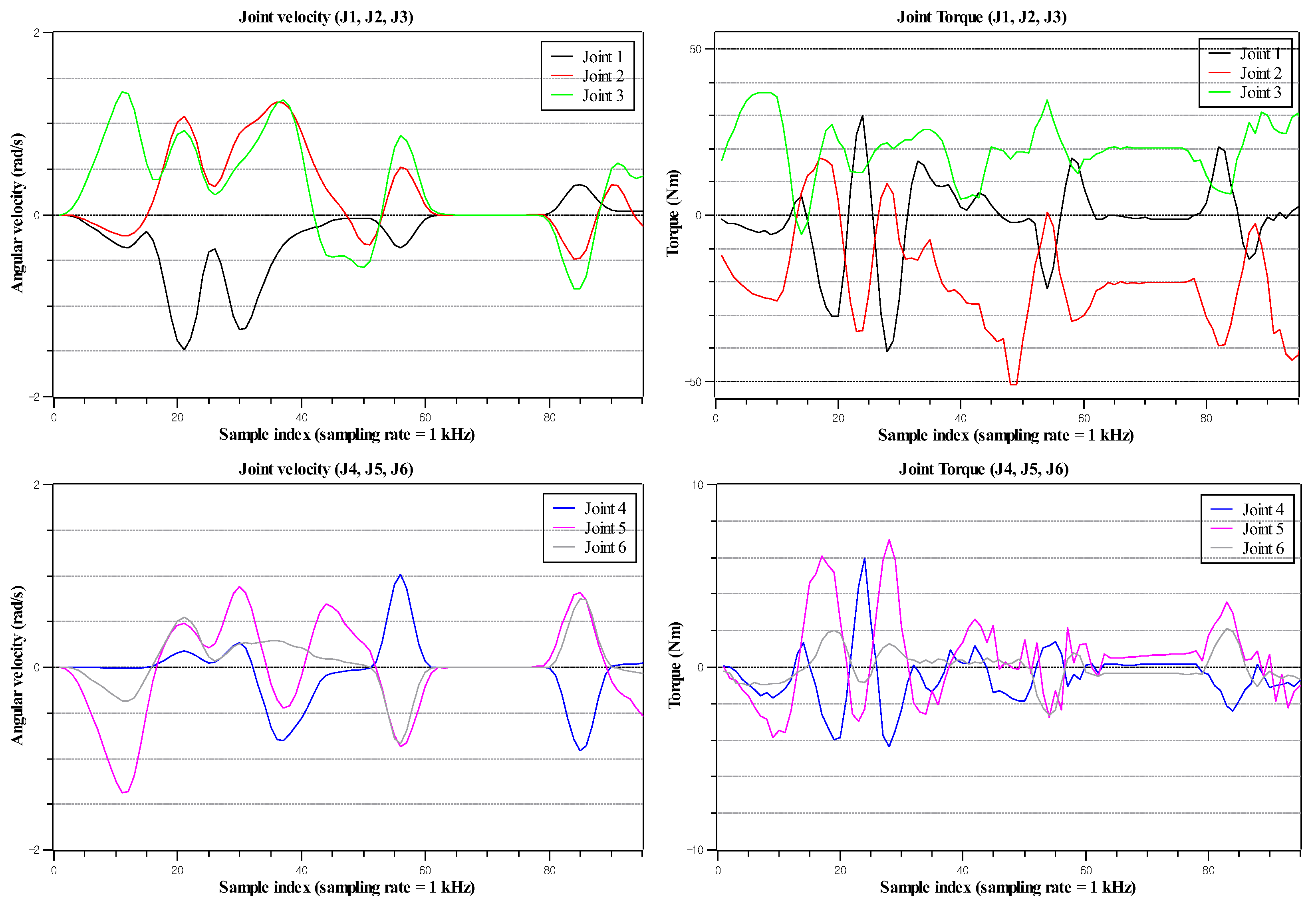
Joint states were recorded during programmed working trajectories covering a broad range of motion for all six joints. The measured signals include joint positions q , velocities q ˙ , accelerations q ¨ , and measured joint torques τ as shown in Figure 5. All joint signals were sampled at 1 kHz to capture transient dynamics and non-conservative effects such as frictional variations. The gear meshing frequencies (GMFs) of the primary gears, including the input, spur, and bevel gears, were calculated to range from 986.4 Hz to 2945.0 Hz. Acoustic measurements confirmed that harmonic components consistently appeared around 1000 Hz, 2000 Hz, 3000 Hz, and 4000 Hz. However, the method proposed in this study primarily relies on estimating the robot dynamics from current, voltage, and joint angle measurements, followed by SHAP-based feature attribution analysis. Therefore, the GMFs themselves are not directly relevant to the analysis. Empirically, the signals were sampled at twice the control cycle frequency of the robot, which was sufficient to capture the dynamics necessary for SHAP-based evaluation. The raw measurements were subsequently denoised using a Savitzky–Golay filter (window length = 500 samples, polynomial order = 3). This filter was selected because it effectively suppresses high-frequency measurement noise while preserving the phase, amplitude, and waveform characteristics of the original motion signals, thereby ensuring representations of the robot’s joint behavior.
All experiments were conducted under standard Korean factory conditions, where indoor temperatures typically range from 10 °C to 35 °C. Since the robots originated from customer production sites and were already in a warmed-up operational state, frictional or power deviations due to ambient temperature were considered negligible. In addition to that, the reducers were intended to be properly lubricated according to the manufacturer’s maintenance manual. However, this could not be independently verified.

3.3. Dataset Composition

The experimental dataset was collected from a variety of industrial robots under both normal and faulty operating conditions. The robots used for data acquisition are fundamentally 6-axis serial-link articulated robots. Each is equipped with an additional wrist-mounted axis that drives a spot-welding gun as an end-effector, making them 7-axis robots in total. All robots are installed in spot-welding processes, with payload capacities ranging from 165 kg to 200 kg. There are no identical robots among them—the dataset includes 15 distinct robot units. All robots are manufactured by (HD Hyundai Robotics Co., Ltd., Daegu, Republic of Korea), with model names HS165 and HS200, which are commonly used in handling and spot-welding operations. Each robot is equipped with a welding gun of different weight and operates at varying speeds—either slow or fast—according to its individual production schedule. In addition, the installation and operating durations differ across robots. Consequently, the dataset used for subsequent training and classification inherently reflects diversity in speed, payload, and noise characteristics.
The dataset includes both testbeds and in-field industrial processes, covering motor brake faults, reducer faults, and normal operation. A summary of the dataset composition is provided in Table 1. In the SHAP-based classification stage, each measurement file—corresponding to a specific operating condition—was used to train an independent dynamics MLP model. SHAP attributions were then computed for all samples within each file, producing one SHAP feature set per file. The resulting feature sets were concatenated (stacked and flattened) into a single dataset used for classification. This aggregated SHAP dataset contained 78,436 samples in total (36,168 normal and 42,268 fault), consistent with the original label distribution shown in Table 1. The final classification MLP was trained using an 80/20 stratified random split to maintain class balance across partitions.

3.4. Implementation Details

The architectures and training hyperparameters of both MLP networks are summarized in Table 2. All models were implemented in Python 3.9.21 using the PyTorch 2.5.0 framework. The MLP-based dynamics model ( f MLP ) was trained using the Adam optimizer with a learning rate of 1 × 10 3 , batch size of 256, and early stopping based on validation loss to prevent overfitting. The subsequent fault-classification MLP, which receives SHAP-based fingerprints as input, was trained for 10,000 epochs with the same optimizer and learning rate but without early stopping. All experiments were conducted on a workstation equipped with an NVIDIA Quadro RTX 8000 GPU.

4. Results and Discussion

4.1. MLP-Based Dynamics Modeling for Feature Attribution

To investigate the predictive performance of neural network models on the system dynamics, we implemented an MLP model. Although the MLP does not achieve the highest possible accuracy compared to more complex architectures such as LSTMs or Transformers, it provides sufficiently accurate predictions to support downstream analyses, particularly for SHAP-based feature attribution.
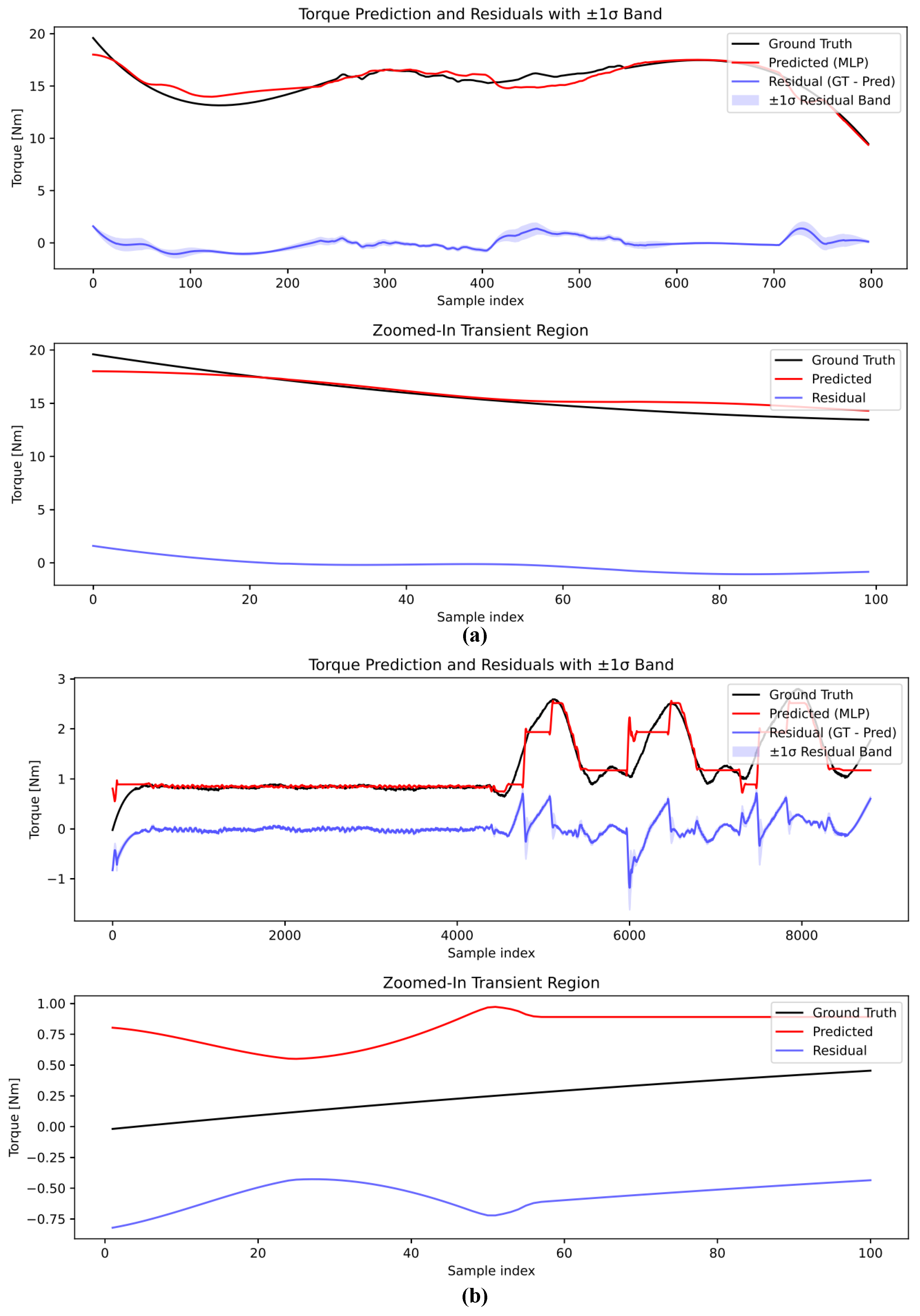
Figure 6 shows the comparison between the observed trajectories and the predictions generated by the MLP. The model captures the overall trends and major transitions in the system dynamics, although minor deviations are present in some segments. These discrepancies highlight the limitations of the MLP in modeling long-term dependencies and subtle temporal patterns, but do not substantially affect its utility for feature contribution analysis. To quantify these deviations, we computed the mean-squared error (MSE) between the predicted and measured joint torques across all datasets. The average MSE was approximately 2.48 × 10 1 Nm2 with a standard deviation of 2.96 × 10 1 Nm2, ranging from 4.0 × 10 2 to 1.0 × 10 2 Nm2 depending on the dynamic conditions as shown in Table 3. These results indicate that the majority of samples achieved sub-unit to low-level errors. Moreover, the average computation time per sample was 6.9 × 10 5 s. Overall, the MLP-based dynamics estimator demonstrates sufficient accuracy and computational efficiency, confirming its suitability for downstream SHAP analysis and practical diagnostic applications.
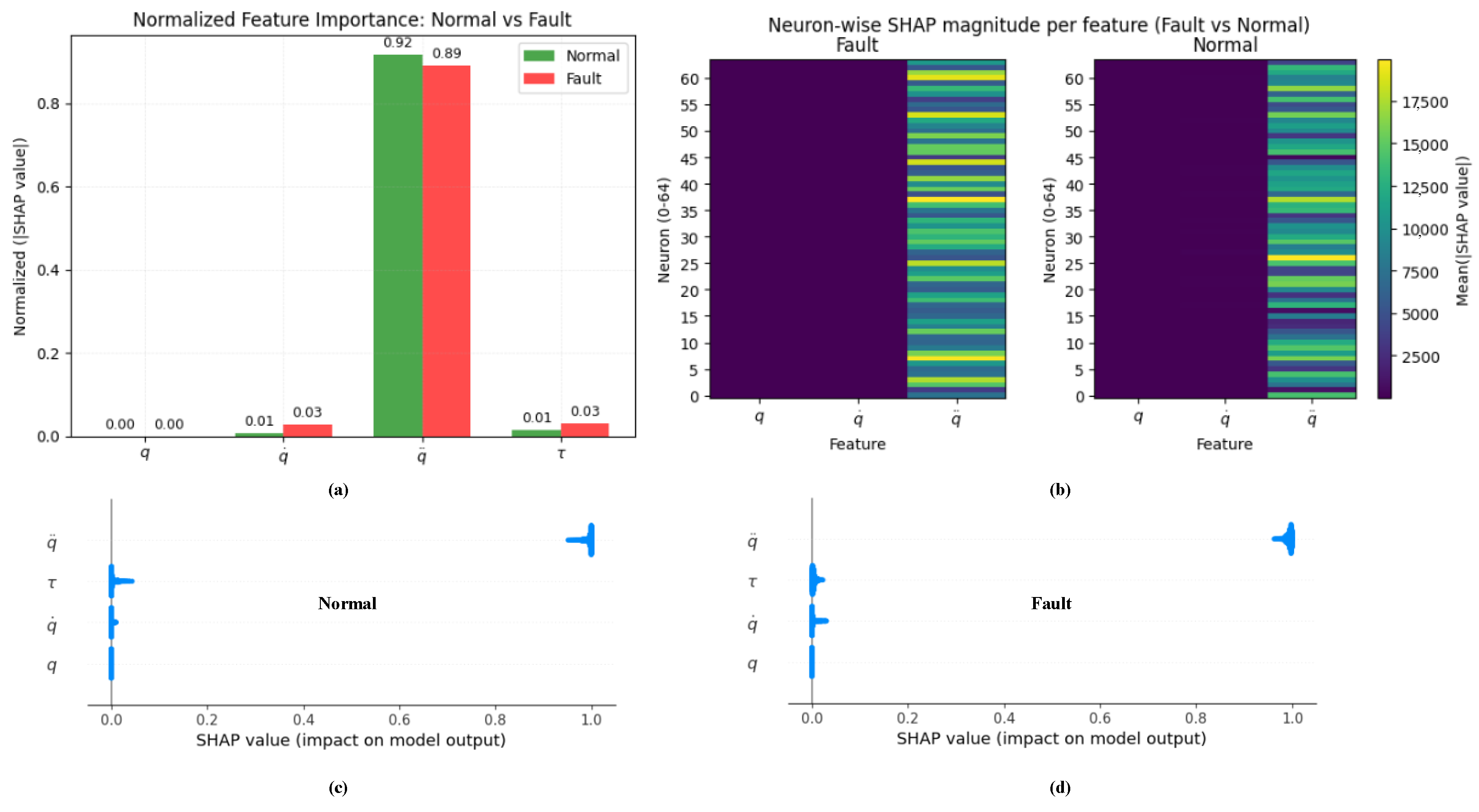
The feature attribution analysis using SHAP provides a quantitative interpretation of how each input variable contributes to the model output. Figure 7 illustrates the SHAP-based interpretability results under both normal and fault conditions. As shown in Figure 7a, the joint acceleration terms ( q ¨ ) exhibit the highest contribution to the model output. In the normal condition, the effect of q ¨ is slightly more pronounced compared to the fault condition, indicating that the model relies more on acceleration-related dynamics when the system operates normally. Conversely, the contribution of the joint velocity terms ( q ˙ ) is relatively higher under the fault condition than in the normal case, implying that velocity-dependent features become more influential when a fault occurs. Figure 7b presents the neuron-wise SHAP attribution, showing that the degree of contribution from individual neurons differs significantly between the normal and fault conditions. This observation suggests that the internal feature encoding of the network changes depending on the system state, reflecting a redistribution of neural activations in response to faults. Figure 7c,d depict the beeswarm plots for each input feature. It can be observed that the distributional patterns of the joint acceleration ( q ¨ ) features differ between the normal and fault conditions. In the fault case, the positive extremes of the SHAP values of q ¨ are smaller than those observed in the normal case, while the negative extremes are increased in magnitude. This indicates that under fault conditions, the acceleration features contribute more in a direction that decreases the predicted joint torque, suggesting that the model adapts its output to mitigate excessive torque when the system experiences a fault. These differences demonstrate that the proposed model effectively distinguishes between normal and faulty behaviors through feature-sensitive representation learning.
Figure 8 presents the SHAP analysis results for all six joints. As shown in Figure 8a, the SHAP values were computed for 24 input features corresponding to the joint position (q), velocity ( q ˙ ), acceleration ( q ¨ ), and torque ( τ ) of six joints. The neuron activation patterns indicate that neurons associated with the acceleration terms of the second and third joints are most prominently activated. From a physical perspective of the robot’s task dynamics, the second and third joints experience the largest gravitational loads, as they act against gravity during operation. In fact, these joints are often equipped with additional spring mechanisms for gravity compensation. Similarly, Figure 8b shows that the acceleration features of the second and third joints exhibit the highest activation, and particularly, the velocity term of the third joint—which bears the heaviest load—also demonstrates strong activation.
By leveraging the MLP in combination with SHAP, we can gain insights into feature-level contributions and classify faults without the additional complexity and computational cost associated with more sophisticated sequence modeling approaches.

4.2. Fault Classification Performance

Table 4 and Table 5 summarize the classification performance of the baseline and proposed methods. The baseline approach, which directly classifies fault states using raw joint positions, velocities, accelerations, and torque ( q , q ˙ , q ¨ , τ ), achieved a maximum accuracy of 97.3% when using Random Forest, while MLP and SVM reached 92–93% accuracy. Logistic Regression performed noticeably worse (89.3% accuracy), reflecting the difficulty of capturing complex nonlinear interactions in the high-dimensional joint signal space. In contrast, the proposed framework, which first estimates an MLP-based dynamics model and then analyzes feature attributions using SHAP fingerprints, yielded substantially improved results. Both MLP and Random Forest achieved near-perfect classification (99.8–100% accuracy), while linear models such as Logistic Regression failed to separate classes effectively (49.9% accuracy), highlighting the necessity of modeling nonlinearity for fault detection. SVM showed intermediate performance (67.7% accuracy), limited by its sensitivity to nonlinear and high-dimensional feature interactions. These findings demonstrate that the SHAP-based feature representation enhances the discriminative ability of subsequent classifiers by explicitly capturing the contribution of each input feature to the system dynamics. The training times remained reasonable, with the proposed MLP completing in approximately 1 s, illustrating the practical feasibility of this approach for diagnostic applications. Although Random Forest achieves slightly higher classification accuracy on the SHAP fingerprints, we selected an MLP for the second-stage classifier due to its scalability and integration potential with end-to-end learning pipelines while maintaining relatively fast training and inference times.
The result in Table 5 is unsurprising, as the SHAP method highlights the most influential terms, and even a human observer can readily distinguish the difference. Attribution analysis further revealed a clear state-dependent shift: healthy operation is characterized by acceleration-sensitive contributions, while faulty states emphasize velocity-related terms, consistent with increased friction and torque fluctuations in the brake and gear mechanisms. These findings confirm that the proposed framework not only achieves high classification accuracy but also captures fault-consistent feature patterns that enhance diagnostic reliability.
Although the inference times of both dynamics MLP and classifier MLP models are shorter than 1 ms, real-time operation at a 1 kHz sampling frequency is practically constrained by the additional computational overhead, such as the generation of SHAP fingerprints and the associated preprocessing steps. Therefore, instead of performing online learning and inference at every control cycle, a more feasible strategy is to periodically update the dynamics MLP model using the joint-state and torque data accumulated over a given interval. The updated model can then be deployed for inference within subsequent control cycles. This periodic training and inference scheme provides feasibility under varying robot job programs and operating conditions.

4.3. Limitations

Although the dataset used in this study was collected from industrial robots operating under real production conditions, it primarily consists of measurements from spot-welding processes in automotive manufacturing. The analysis therefore depends on the representativeness of this specific task domain. Moreover, the method relies on sensor inputs such as current sensors and encoders, meaning that sensor degradation, improper sensitivity calibration, or scale-setting errors could lead to biased or inaccurate results.
In addition, the proposed framework has not yet been fully validated under simultaneous multi-fault conditions. Nevertheless, since the approach focuses on identifying robot dynamics and analyzing feature attribution of torque responses to joint states, it is not limited to a single fault type. The framework has the potential to detect a wide range of fault phenomena—including increased friction due to insufficient lubrication, transmission variation caused by gear surface damage, reducer wear-out, bearing degradation, or tension misadjustment. However, further investigation is required to categorize and quantify these fault types in a unified diagnostic framework.

5. Conclusions

This study presented a dynamics-model-informed, feature-guided fault diagnosis framework for industrial robot manipulators, leveraging neural networks and SHAP-based feature analysis. By modeling robot dynamics with a data-driven multi-layer perceptron and analyzing the contribution of input features, the proposed method successfully distinguished between normal and faulty conditions. Experimental validation on real-world datasets, including both motor brake and reducer faults, demonstrated that the framework achieves near-perfect classification performance while capturing fault-consistent feature patterns.
If a robot has already reached an inoperable state, it is too late to apply this methodology. The present study focuses on detecting subtle contributions of inputs and outputs in an operating robot to diagnose faults. In other words, it identifies early signs of faults—localized modifications—that may eventually evolve into critical failures. Maintenance activities can be classified into scheduled offline inspections and online condition monitoring; the proposed method is suitable for online application. In practical deployment on real robots, the method successfully detected anomalies. For such mechanisms, although the robot remains operational, empirically, there is a high likelihood of a critical failure occurring within six to twelve months. Moreover, even before major failures occur, issues such as increased backlash or abnormal power consumption may arise, indicating that immediate disassembly and inspection are required upon detecting these early signs. In addition to the existing PLC/SCADA network in a factory setting, this study leverages fundamental robot control signals, such as motor currents and joint angles. Therefore, as long as the robot controller provides a protocol to transmit these signals externally, the proposed method can be integrated using the existing network infrastructure.
For future work, we plan to enhance torque estimation by employing physics-informed neural networks (PINNs) that incorporate both conservative and non-conservative forces to constrain the MLP or other neural network models. In addition, to disambiguate faults in the reducer, bearings, and belt tension, we will explore a vibration and acoustic signal fusion approach. This strategy is motivated by the observation that experienced engineers can often infer the location and type of fault solely from audible signals; achieving comparable diagnostic capability is therefore a primary objective of this research.

Funding

This research received no external funding.

Institutional Review Board Statement

Not applicable.

Informed Consent Statement

Not applicable.

Data Availability Statement

The raw data supporting the conclusions of this article are company confidential; access may be granted upon reasonable request subject to review by the author.

Conflicts of Interest

The author declares no conflicts of interest.

Nomenclature

SymbolDescriptionUnit
qJoint position vectorrad
q ˙ Joint velocity vectorrad/s
q ¨ Joint acceleration vectorrad/s2
τ Joint torqueNm
M ( q ) Inertia matrixkg·m2
C ( q , q ˙ ) Coriolis/centrifugal matrixNm
g ( q ) Gravity torque vectorNm
τ f r i c Friction torqueNm
τ e r r Torque estimation errorNm
θ Joint angle (encoder reading)rad
η ( t ) Sensor error/noise at time tunit depends on sensor
ϕ i SHAP feature contribution for feature i-
Φ SHAP vector for all features-
f ( · ) MLP model output function-
LLoss function used for training-

References

  1. Shi, G.; Nigatu, H.; Wang, Z.; Huang, Y. DNN-Augmented Kinematically Decoupled Three-DoF Origami Parallel Robot for High-Precision Heave and Tilt Control. Actuators 2025, 14, 291. [Google Scholar] [CrossRef]
  2. Jia, L.; Chen, K.; Liao, Z.; Qiu, A.; Cao, M. Adaptive Robust Impedance Control of Grinding Robots Based on an RBFNN and the Exponential Reaching Law. Actuators 2025, 14, 393. [Google Scholar] [CrossRef]
  3. Lu, C.; Gao, R.; Yin, L.; Zhang, B. Human–robot collaborative scheduling in energy-efficient welding shop. IEEE Trans. Ind. Inform. 2023, 20, 963–971. [Google Scholar] [CrossRef]
  4. Liu, Z.; Cheng, S.; Su, Y.; Duan, G.; Tan, J. Semantic Segmentation Based Spraying Trajectory Planning for Complex Product. IEEE Trans. Ind. Inform. 2024, 20, 9416–9426. [Google Scholar] [CrossRef]
  5. Deng, X.; Liu, J.; Gong, H.; Gong, H.; Huang, J. A human–robot collaboration method using a pose estimation network for robot learning of assembly manipulation trajectories from demonstration videos. IEEE Trans. Ind. Inform. 2022, 19, 7160–7168. [Google Scholar] [CrossRef]
  6. Cao, B.; Yu, J.; Zhang, Y.; Liu, P.; Zhang, Y.; Sun, H.; Jin, P.; Lin, J.; Wang, L. A Novel Kinematic Calibration Method for Industrial Robots Based on the Improved Grey Wolf Optimization Algorithm. Actuators 2025, 14, 403. [Google Scholar] [CrossRef]
  7. Kim, H.; Jeong, H.; Lee, H.; Kim, S.W. Online and offline diagnosis of motor power cables based on 1d cnn and periodic burst signal injection. Sensors 2021, 21, 5936. [Google Scholar] [CrossRef]
  8. Kim, H.; Lee, H.; Kim, S.; Kim, S.W. Attention recurrent neural network-based severity estimation method for early-stage fault diagnosis in robot harness cable. Sensors 2023, 23, 5299. [Google Scholar] [CrossRef]
  9. Sabry, A.H.; Nordin, F.H.; Sabry, A.H.; Ab Kadir, M.Z.A. Fault detection and diagnosis of industrial robot based on power consumption modeling. IEEE Trans. Ind. Electron. 2019, 67, 7929–7940. [Google Scholar] [CrossRef]
  10. Buhari, M.; Levi, V.; Awadallah, S.K. Modelling of ageing distribution cable for replacement planning. IEEE Trans. Power Syst. 2015, 31, 3996–4004. [Google Scholar] [CrossRef]
  11. Shirkoohi, G. Modelling of fault detection in electrical wiring. IET Sci. Meas. Technol. 2015, 9, 211–217. [Google Scholar] [CrossRef]
  12. Lundquist, E.J.; Nagel, J.R.; Wu, S.; Jones, B.; Furse, C. Advanced forward methods for complex wire fault modeling. IEEE Sens. J. 2012, 13, 1172–1179. [Google Scholar] [CrossRef]
  13. Kim, H. Robot dynamics-based cable fault diagnosis using stacked transformer encoder layers. Electr. Eng. 2024, 107, 3697–3708. [Google Scholar] [CrossRef]
  14. He, Y.; Chen, J.; Zhou, X.; Huang, S. In-situ fault diagnosis for the harmonic reducer of industrial robots via multi-scale mixed convolutional neural networks. J. Manuf. Syst. 2023, 66, 233–247. [Google Scholar] [CrossRef]
  15. Chen, C.; Liu, C.; Wang, T.; Zhang, A.; Wu, W.; Cheng, L. Compound fault diagnosis for industrial robots based on dual-transformer networks. J. Manuf. Syst. 2023, 66, 163–178. [Google Scholar] [CrossRef]
  16. Kim, H.; Lee, H.; Kim, S.W. Current only-based fault diagnosis method for industrial robot control cables. Sensors 2022, 22, 1917. [Google Scholar] [CrossRef]
  17. Zhao, R.; Yan, R.; Wang, J.; Mao, K.; Shen, P.; Wang, X. Deep learning and its applications to machine health monitoring: A survey. Mech. Syst. Signal Process. 2019, 115, 213–237. [Google Scholar] [CrossRef]
  18. Liu, J.; Borja, P.; Della Santina, C. Physics-informed neural networks to model and control robots: A theoretical and experimental investigation. Adv. Intell. Syst. 2024, 6, 2300385. [Google Scholar] [CrossRef]
  19. Meng, C.; Griesemer, S.; Cao, D.; Seo, S.; Liu, Y. When physics meets machine learning: A survey of physics-informed machine learning. Mach. Learn. Comput. Sci. Eng. 2025, 1, 20. [Google Scholar] [CrossRef]
  20. Guc, F.; Chen, Y. Sensor fault diagnostics using physics-informed transfer learning framework. Sensors 2022, 22, 2913. [Google Scholar] [CrossRef]
  21. Uhrich, B.; Pfeifer, N.; Schäfer, M.; Theile, O.; Rahm, E. Physics-informed deep learning to quantify anomalies for real-time fault mitigation in 3D printing. Appl. Intell. 2024, 54, 4736–4755. [Google Scholar] [CrossRef]
  22. Ni, R.; Qureshi, A.H. Progressive learning for physics-informed neural motion planning. arXiv 2023, arXiv:2306.00616. [Google Scholar] [CrossRef]
  23. Qi, X.; Wang, S.; Fang, C.; Jia, J.; Lin, L.; Yuan, T. Machine learning and SHAP value interpretation for predicting comorbidity of cardiovascular disease and cancer with dietary antioxidants. Redox Biol. 2025, 79, 103470. [Google Scholar] [CrossRef]
  24. Gawde, S.; Patil, S.; Kumar, S.; Kamat, P.; Kotecha, K.; Alfarhood, S. Explainable predictive maintenance of rotating machines using lime, shap, pdp, ice. IEEE Access 2024, 12, 29345–29361. [Google Scholar] [CrossRef]
  25. Lin, K.; Gao, Y. Model interpretability of financial fraud detection by group SHAP. Expert Syst. Appl. 2022, 210, 118354. [Google Scholar] [CrossRef]
  26. Lundberg, S.M.; Lee, S.I. A Unified Approach to Interpreting Model Predictions. In Proceedings of the Advances in Neural Information Processing Systems (NeurIPS), Long Beach, CA, USA, 4–9 December 2017; Volume 30. [Google Scholar]
  27. Jang, K.; Pilario, K.E.S.; Lee, N.; Moon, I.; Na, J. Explainable artificial intelligence for fault diagnosis of industrial processes. IEEE Trans. Ind. Inform. 2023, 21, 4–11. [Google Scholar] [CrossRef]
  28. Jeon, J.E.; Hong, S.J.; Han, S.S. Utilization of Machine Learning and Explainable Artificial Intelligence (XAI) for Fault Prediction and Diagnosis in Wafer Transfer Robot. Electronics 2024, 13, 4471. [Google Scholar] [CrossRef]
  29. Zereen, A.N.; Das, A.; Uddin, J. Machine Fault Diagnosis Using Audio Sensors Data and Explainable AI Techniques-LIME and SHAP. Comput. Mater. Contin. 2024, 80, 3463–3484. [Google Scholar] [CrossRef]
  30. Brusa, E.; Cibrario, L.; Delprete, C.; Di Maggio, L.G. Explainable AI for machine fault diagnosis: Understanding features’ contribution in machine learning models for industrial condition monitoring. Appl. Sci. 2023, 13, 2038. [Google Scholar] [CrossRef]
  31. Dahl, P.R. A Solid Friction Model; Technical Report; PubGenius Inc.: Milpitas, CA, USA, 1968. [Google Scholar]
  32. Karnopp, D. Computer simulation of stick-slip friction in mechanical dynamic systems. J. Dyn. Syst. Meas. Control. 1985, 107, 100–103. [Google Scholar] [CrossRef]
  33. Haessig, D.A., Jr.; Friedland, B. On the modeling and simulation of friction. In Proceedings of the 1990 American Control Conference, San Diego, CA, USA, 23–25 May 1991. [Google Scholar]
  34. Corke, P.I. A simple and systematic approach to assigning Denavit–Hartenberg parameters. IEEE Trans. Robot. 2007, 23, 590–594. [Google Scholar] [CrossRef]
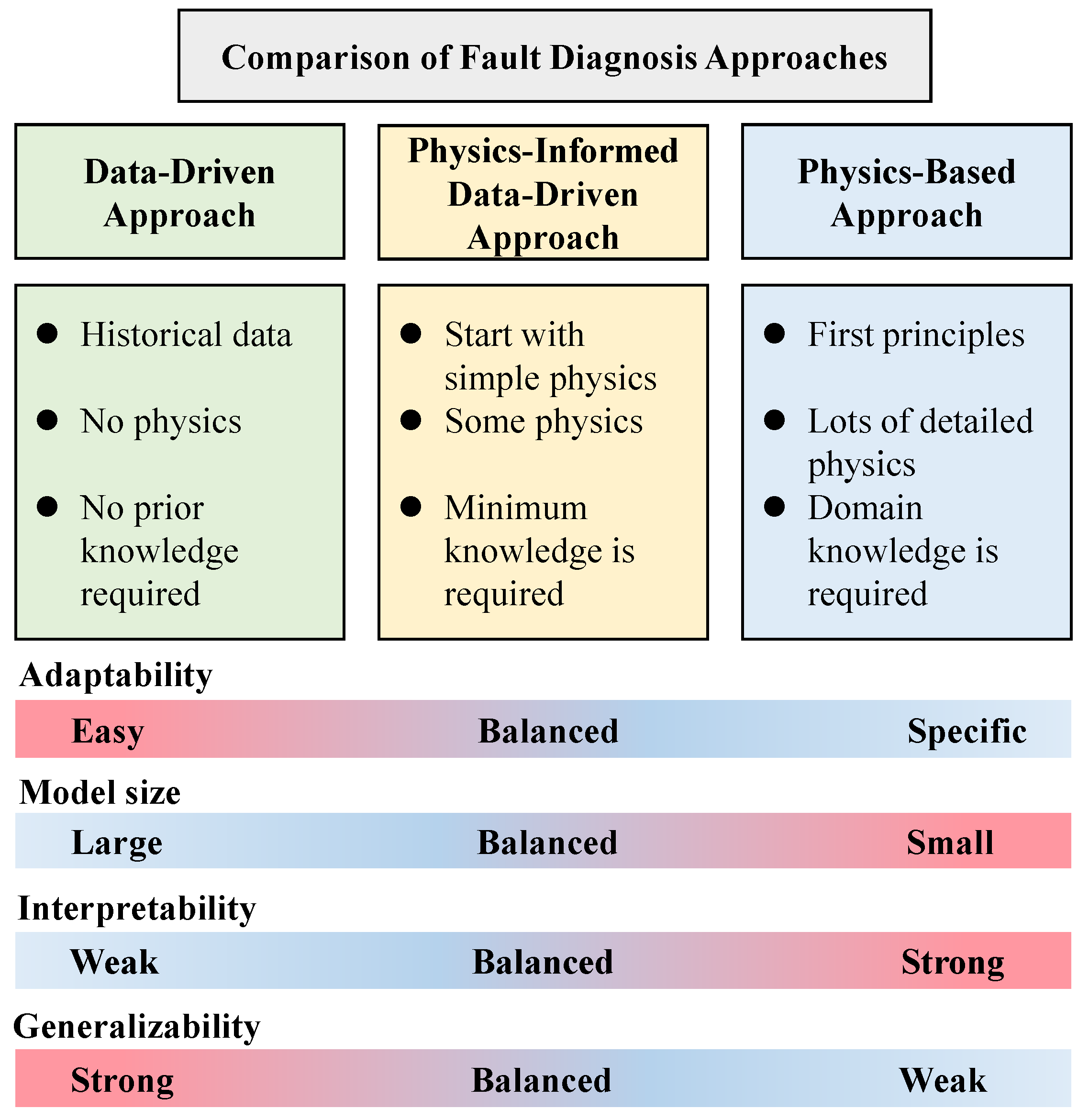
Figure 1. Conceptual comparison of diagnostic approaches. The proposed hybrid SHAP-informed method combines the interpretability of model-based analysis and the flexibility of data-driven learning. The trade-off between interpretability and generality is balanced by incorporating residual dynamics modeling and SHAP-based explainability.
Actuators 14 00583 g001
Figure 2. The overall workflow of the proposed fault diagnosis method.
Actuators 14 00583 g002
Figure 3. Mechanical structure of the industrial robot and motor–reducer assembly.
Actuators 14 00583 g003
Figure 4. The real robot installed in the production process and their faulty reducer and gear.
Actuators 14 00583 g004
Figure 5. Measured joint angular velocities and torques of six robot joints. Subplots show velocity and torque profiles for joints J1–J3 and J4–J6 under the normal condition. Each signal was sampled at 1 kHz and smoothed using a Savitzky–Golay filter.
Actuators 14 00583 g005
Figure 6. Comparison between observed system trajectories (black), MLP-predicted trajectories (red), and residuals (blue) in normal operation conditions. (a) presents the estimated torque of the brake rig, while (b) shows the estimated torque of the industrial robot used in this study. The MLP captures the overall trend, providing a reasonable approximation for downstream feature attribution analysis using SHAP. The negative torque observed in certain regions is attributed to regenerative effects when the robot joints move along the direction of gravity.
Actuators 14 00583 g006
Figure 7. SHAP-based interpretability analysis under normal and fault conditions. (a) Normalized feature importance of q, q ˙ , and q ¨ . (b) Neuron-wise SHAP attribution maps showing the distribution of activation strengths across 64 latent neurons. (c,d) Beeswarm plots illustrating the feature-level SHAP distributions under normal and fault conditions, respectively.
Actuators 14 00583 g007
Figure 8. SHAP analysis results for each of the six robot joints. (a) shows the SHAP values of 24 input features, consisting of position (q), velocity ( q ˙ ), acceleration ( q ¨ ), and torque ( τ ) for six joints. Neurons corresponding to the acceleration terms of the 2nd and 3rd joints exhibit dominant activation, which aligns with the fact that these joints experience the largest gravitational loads during motion. (b) also highlights strong activation in the acceleration and velocity terms of the 3rd joint, which bears the heaviest dynamic load in the manipulator structure.
Actuators 14 00583 g008
Table 1. Summary of dataset composition.
CategoryTest Env.TypeApplicationCap./PayloadSamples
Brake FaultsTest Rig 1Brake FaultJoint 4–62.0 kW12,324
Test Rig 2Brake FaultJoint 1–34.3 kW7135
Test Rig 3Brake FaultJoint 1–34.3 kW7135
Test Rig 4NormalJoint 4–62.0 kW11,084
Test Rig 5NormalJoint 4–62.0 kW8799
Test Rig 6NormalJoint 1–34.3 kW7135
Test Rig 7NormalJoint 1–34.3 kW7140
Reducer FaultsProcess 1, 2, 3, 4NormalSpot welding165 kg4665
Process 5, 6, 7, 8Reducer FaultSpot welding165 kg5236
Process 9NormalSpot welding165 kg892
Process 10, 11Reducer FaultSpot welding165 kg2519
Process 12, 13NormalSpot welding165 kg1893
Process 14Reducer FaultSpot welding200 kg1426
Process 15Reducer FaultSpot welding165 kg1053
Total78,436
Table 2. Architectures and hyperparameters of MLP models used for dynamics modeling and fault classification.
ItemSpecification
MLP #1
InputState ( q , q ˙ , q ¨ ) per joint
Hidden layers2 fully connected layers: [64, 64] neurons
Activation functiontanh for hidden layers; linear for output
Batch size256 samples per minibatch
OptimizerAdam
Learning rate 1 × 10 3
Loss functionMean squared error (MSE)
Number of epochs1000 (max training iterations)
Early stoppingPatience = 20 epochs (validation loss)
Random seedFixed (seed = 42)
MLP #2
InputSHAP-based feature vector per joint
Hidden layers2 fully connected layers: [64, 32] neurons
Activation functionsReLU for hidden layers; Sigmoid for output
Output dimension1 (binary: normal/fault)
Loss functionBinary cross-entropy (BCE)
OptimizerAdam
Learning rate 1 × 10 3
Batch sizeFull-batch (entire dataset)
Number of epochs10,000
Early stoppingNot applied
Random seedFixed (seed = 42)
Table 3. Torque prediction errors and computation time per sample for 22 test cases.
SampleTorque MSE (Nm2)RMSE (Nm)Comp. Time per Samples (s)
17.009 × 10 1 8.376.353 × 10 5
24.151 × 10 1 6.445.634 × 10 5
36.742 × 10 1 8.216.316 × 10 5
44.121 × 10 1 6.426.760 × 10 5
52.8341.689.300 × 10 5
62.342 × 10 1 4.846.303 × 10 5
73.8891.977.115 × 10 5
83.492 × 10 1 0.591.338 × 10 4
92.101 × 10 1 0.467.952 × 10 5
107.922 × 10 1 0.895.648 × 10 5
112.2741.517.915 × 10 5
124.251 × 10 1 6.528.365 × 10 6
135.815 × 10 1 7.631.359 × 10 5
141.002 × 10 2 10.011.311 × 10 5
151.0561.037.753 × 10 6
164.016 × 10 2 0.209.753 × 10 6
171.755 × 10 1 0.421.310 × 10 5
182.523 × 10 1 0.501.532 × 10 5
192.4811.571.293 × 10 4
201.674 × 10 1 4.097.754 × 10 5
212.6231.625.650 × 10 5
224.498 × 10 1 0.677.234 × 10 5
Table 4. Baseline classification using raw joint signals using 5-fold cross-validation (Mean ± Std).
ModelAccuracyAUCTraining Time [s]Inference Time [s]
Random Forest0.973 ± 0.0020.998 ± 0.0006.224 ± 0.0880.117 ± 0.008
MLP0.925 ± 0.0020.986 ± 0.0012.082 ± 0.0470.001 ± 0.001
SVM0.922 ± 0.0020.983 ± 0.001145.582 ± 1.78812.334 ± 0.115
Logistic Regression0.893 ± 0.0030.938 ± 0.0020.028 ± 0.0010.001 ± 0.001
Table 5. Comparison of classifiers on SHAP fingerprints using 5-fold cross-validation (Mean ± Std).
ModelAccuracyAUCTraining Time (s)Inference Time [s]
Random Forest1.000 ± 0.0001.000 ± 0.0004.180 ± 0.082 2.036 × 10 5 ± 1.386 × 10 6
MLP0.998 ± 0.0030.998 ± 0.0051.048 ± 0.016 4.528 × 10 7 ± 6.200 × 10 7
SVM0.677 ± 0.0160.785 ± 0.0218.350 ± 0.162 7.856 × 10 4 ± 2.414 × 10 5
Logistic Regression0.499 ± 0.0230.532 ± 0.0111.580 ± 0.025 1.131 × 10 6 ± 4.018 × 10 10
Disclaimer/Publisher’s Note: The statements, opinions and data contained in all publications are solely those of the individual author(s) and contributor(s) and not of MDPI and/or the editor(s). MDPI and/or the editor(s) disclaim responsibility for any injury to people or property resulting from any ideas, methods, instructions or products referred to in the content.