


Abstract
Many studies of human migration focus on modern issues such as economics, politics, urbanization, and commuting. Here, we seek foundational patterns by using very large genealogies to measure migration centuries before modern technologies or census data became available. In Europe and North America from 1400 to 1950 we find two distinct patterns of internal lifetime migration: in most locations and eras we find “steady-state” migration with a power–law distribution of migration distance. A very different “frontier” distribution appears suddenly in North America after 1740; it is not a simple power law and has much longer average distances. All datasets (both patterns) are well fit by a three-parameter model; the temporal and geographic patterns of the fitted parameters give new insight to American internal expansion 1620–1950. In addition, we find that frontier migration is highly directional and asymmetric; gravity models do not apply. The American frontier pattern arises from the colonial-era steady-state within two generations, plateaus, and then returns to a more mobile steady-state. This frontier pattern is enabled by large-scale technological or numeric imbalance and geographic opportunity; when these forces abate, a new steady-state begins.
1. Introduction
Humans must have a way to physically survive in order to live in a particular place. Food and shelter are paramount, but the processes by which people have supported themselves across the diverse habitats of the world have varied in countless ways over the centuries. At times, necessity or opportunity has resulted in migrations of individuals and families from one locale to another, to a destination near their current home or hundreds of miles away. The patterns and processes of human migration have been studied by scholars around the globe focusing on various historical periods and places. Their studies have resulted in a nearly endless array of articles and books that aim to discover the main patterns and processes of life-course migration and even multi-generational migration. In this paper, we propose a model of migration that combines a limited set of variables that describe the timing and geographical spread of migrants historically. We use a rich genealogical dataset (Kaplanis et al. 2018) to illustrate the applicability of our model to various places and during different periods.
Analyzing migration patterns has often been limited by the amount and quality of population data. Census records and other government compilations, such as birth or death records, have been used extensively, but they are limited in that they are just a snapshot of people at one time. However, in some censuses, for example, the birth location of an individual and their parents is included (like the 1880 US Census) along with a location for where the person resided at that time, which therefore gives a two-generation data picture of migration at that point. US censuses can also have some other characteristics that increase their value, such as socio-economic variables like income, education, occupation and other variables such as race and spoken language depending on what is on the census forms. As such, using censuses and other government vital records as data sources to study migration within the US (e.g., Hudson 1988, 2024; Swierenga 1989; Arreola and Hartwell 2014) and other nations, such as Canada and Great Britain (Hornsby 1992; Hinde 2004), has been common practice for many years.
To better utilize the value of censuses in migration research, scholars have explored the potential of linking multiple sets of records together, such as subsequent censuses. This has been a valuable approach, but it also has limitations. Some of the limitations are underreporting of certain populations, mistakes in records caused by the census takers or enumerated individuals, and other issues such as missing people between censuses (Knights 1991a; Anderson 1988; Anderson and Fienberg 1997; Anderson 2019; Winchester 1970; Hershberg et al. 1976; Markoff and Shapiro 1973; Ruggles et al. 2018; Pouyez et al. 1983). Notwithstanding these challenges, researchers have used linked records and comparisons among censuses, to help them study topics such as historical migration (Thernstrom and Knights 1970; Steckel 1988), the identification of individuals with common names and fake records (Abramitzky et al. 2025; Duzett et al. 2025), economic and social mobility over time (Thernstrom 1973; Otterstrom et al. 2022; Ward et al. 2025), growth in ethnic neighborhoods (Chudacoff 1973; Conzen 1979), cultural diffusion (Waters et al. 2007; Ueda 2017), and community population structure and urban history (Chudacoff 2014; Knights 1971; Knights 1991b; Conzen 1981).
Furthermore, at exceptionally large scales, scholars have mined databases of demographic data to analyze the varied bilateral migration patterns among countries around the world (Abel 2013; Abel and Sander 2014; Abel and Cohen 2019, 2022). Genealogical databases have also allowed more accurate linking of censuses so that genealogy datasets and linked records can be used together to study historical U.S. populations (Koylu et al. 2020, 2025; Price et al. 2021; Buckles et al. 2023).
Others have recognized the value of genealogical data for population research (e.g., Mineau et al. 1989; Adams et al. 2002) though the small sizes of genealogical datasets and issues of data quality have raised concerns about accuracy and bias. However, genealogical data have increasingly been used in population and migration research as the size and quality of genealogy datasets have grown and technology improved (e.g., Otterstrom and Bunker 2013; Koylu et al. 2014; Han et al. 2017; Kaplanis et al. 2018; Koylu and Kasakoff 2022). The Kaplanis data used in this study have been extensively analyzed and validated by the authors and others (Supplementary Material SM1, Chong et al. 2022, Colasurdo and Omenti 2024, Stelter and Alburez-Gutierrez 2022).
Here, we focus on internal migration, and in particular how the distributional properties of a single measurement—lifetime migration distance as recorded by birth and death dates and locations in each person’s genealogic profile—can be accurately fit to a three-parameter model. These distance parameters, supplemented by directionality and symmetry measures derived from the same profiles, reveal a unique pattern that coincides with the era of American westward expansion. Our use of genealogical data is key: its precision—individuals’ specific dates and locations at a 10 km scale—allows us to see complete distributions and build a comprehensive distance model. Its quantity permits the analysis of temporal and geographic subsets which, by correlation to known history, allows us to interpret the numeric results. Censuses alone, and even linked censuses, simply do not have such information in a readily usable form.
The sequence of this paper follows our path of discovery following a discussion of Data Sources and Methods (Section 2) as follows:
- Results: Data Opportunity (Section 3.1): With an interest in human migration, we realize that genealogic data might provide insights into large-scale patterns of migration from pre-technologic societies to the modern era.
- Precedent (Section 3.2): The distribution of city sizes has been consistent across cultures for at least two thousand years, which eliminates technological explanations and forces consideration of more fundamental and universal determinants of human behavior.
- Discovery (Section 3.3): The distribution of lifetime migration distance, derived from genealogies, is also follows a consistent pattern from the medieval to modern eras.
- Exception (Section 3.4): There is a strong exception to this pattern in North American internal migration after 1740.
- Modeling (Section 3.5): A three-parameter mathematical model is developed which explains the full range of observations.
- Slice by Time and Geography (Section 3.6 and Section 3.7): From subsets of genealogic profiles, we can calculate the migration distance parameters over fine slices of time and geography, constraining the exception (Section 3.4) and revealing other trends.
- Additional Metrics (Section 3.8 and Section 3.9): Two additional numerical parameters, migration vector orientation and symmetry, have patterns that correlate with the distance exception and therefore contribute to its interpretation.
- Discussion: Interpreting the Primary Pattern (Section 4.1): The 1/r distribution of migration distance is the backdrop for all migration, and its pre-technological appearance precludes most causation hypotheses in the literature.
- Interpreting the Numerical Parameters (Section 4.2, Section 4.3, Section 4.4, Section 4.5 and Section 4.6): Granular decomposition by time and geography places each parameter in a historical context and suggests the human decisions and actions that drive them.
- Collecting (Section 4.7): All parameter values and properties are summarized as either “steady-state” or “frontier” migration.
- Validation by Mapping (Section 4.8): Maps of our parameters, especially migration symmetry, parallel classic maps of the American frontier.
- Implications (Section 4.9): Our numerical model of frontier migration has implications for individual behavior.
- Other Examples (Section 4.10): Other non-American examples and counter examples clarify the frontier-vs-steady-state distinction.
- Additional Research (Section 4.11): Large genealogies and the statistical tools developed here suggest additional avenues for research.
- Conclusions (Section 5): We offer a summation of the significance and applicability of our findings.
2. Data Sources and Methods
Our sources are the curated and anonymized FamiLinx dataset derived from crowdsourced genealogies (Kaplanis et al. 2018) and the US census study of Sprung-Keyser et al. (2022). Each genealogic profile includes birth and death location by latitude and longitude, from which we calculated lifetime migration distance in kilometers. We recognize that there has been a great deal of intercontinental migration, and even back-and-forth movement between continents during a lifetime (return migration). However, unless otherwise noted, only internal migration (i.e., not ocean-crossing) is considered; otherwise, additional parameter(s) would be required that would add complexity and bias. For example, migration to the United States from the United Kingdom is not included, because that would greatly change the lifetime migration distance values, and so they would not be easily comparable with other birth death distance statistics. For parameter estimation, subsets of Kaplanis are selected by geography and date, and those profiles’ distances are tallied into logarithmic bins, summed, and normalized to give cumulative distribution functions (CDF). Fitting to Equation (1) is by Nelder-Mead optimization with values above 90% excluded to avoid end-of-migration-range truncation. All fits have a rms error <4%. On probability density function (PDF) and CDF plots, the datapoints have no error bars because they are simply counts of genealogy profiles. In order to compare time-slice analysis and mapping to traditional census-based analysis, genealogic profiles should be counted in a way that reasonably corresponds to a census, thus for a given “tally year” and geographic block, we count those born in that block if aged 20 years or younger at that tally year, and those who died in that block if aged over 20 years (Rogers and Castro 1981).
All analyses and mapping were performed using original source code (RWS) without the use of libraries or AI; this code, maps, and links to primary data sources may be found at https://scaledinnovation.com/gg/migration/migration.html (accessed on 11 January 2026).
3. Results
3.1. Inferences from Pre-Industrial Data
Cellphone, social media, and financial transaction datasets have transformed 21st century demography (Deville et al. 2014; Blazquez and Domenech 2018; Barbosa et al. 2018) and unsurprisingly these observations are often interpreted in the context of a modern technological society. Large crowd-sourced genealogies are the inverse: they are generally unsatisfactory resources for events after about 1950 because privacy considerations generally exclude living individuals and their immediate relatives. But by reaching long before the Industrial Revolution, genealogies can reveal patterns that pre-date industrial and urban transitions. These patterns cannot have origins in modern communications, technology, or transportation, but must reflect something less technological and more universal about human behavior. If an early pattern persists in recent datasets, then parsimony suggests that the pre-industrial rationale should prevail. Before discussing human migration, we briefly note such a case for the oldest-known distribution in demography.
3.2. Demographic Parallel in City Sizes
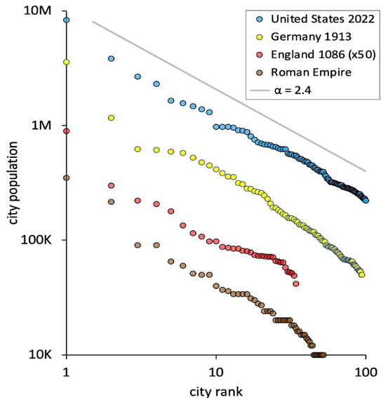
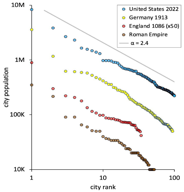
Auerbach (1913) first noted the long-tailed distribution of city sizes. As shown in Figure 1, the pattern spans at least two millennia from the cities of the Roman Empire to early medieval England, to the modern era. Most of the literature devoted to this pattern focuses on recent data and seeks explanations in classical economic terms, in which well-informed, rational actors move to improve their economic wellbeing (Gabaix and Ioannides 2004; Batty 2013).
Figure 1.
Examples of rank-size distributions for city sizes, ancient to modern. The gray line is a power-law function with exponent −2.4, which is typical of these distributions. See Spencer (2024) and http://scaledinnovation.com/gg/cityGrowth.html (accessed on 11 January 2026) for datasets, curve fitting, and source code.
The antiquity of the pattern argues for a different and universal alternative, namely, that the power-law distribution is simply the result of children making the inevitable decision to stay or leave home as they reach adulthood (Spencer 2024). If they stay (historically the majority decision), their own headcount attaches to their birth location, which is the preferential attachment that drives the power law, and if they leave, they seed (or contribute to) another community. This model is self-initializing, unlike a city-to-city migration model, so it is timeless and applicable from the earliest fixed settlements. The exponent of the power law is a simple function of the stay-vs-leave probability and is always greater than two, as observed.
3.3. A Universal Pattern of Migration
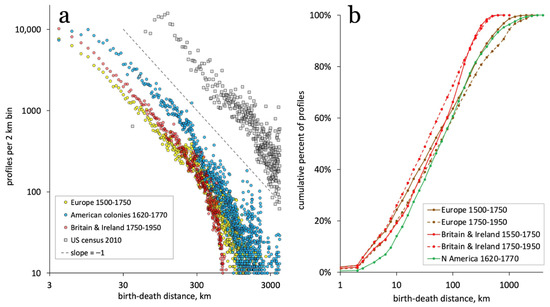
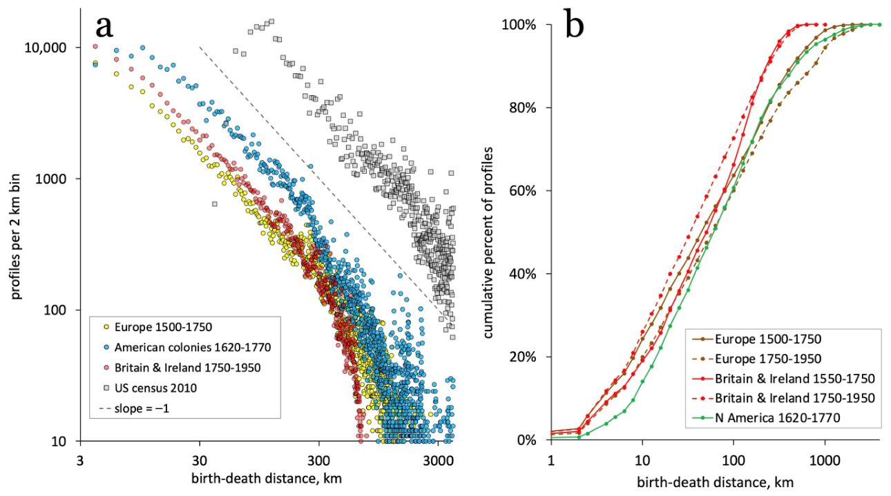
Like city sizes, our datasets reveal a demographic distribution that is centuries older than usually recognized or rationalized. In this case, the relevant metric is not city size, but lifetime migration distance as measured by genealogic birth and death locations. Figure 2a shows the distribution of this distance for 1.1 million Kaplanis profiles plus 9.8 million US census profiles with a result that is universal across continents and centuries: migration distance follows a power law with the exponent −1: the probability that a person has a given lifetime migration distance is inversely proportional to that distance. The same data (with additional time slices) are shown in Figure 2b as normalized cumulative distributions of those who moved at least 1 km, where normalization makes the consistency across continents and centuries more evident. As the integral of 1/x is ln(x), these datasets should be predominantly linear in the cumulative semilog presentation of Figure 2b, as observed.
Figure 2.
(a). A: Circles: distribution of birth-death distance, excluding trans-continental migration, for the indicated regional and temporal subsets of the Kaplanis dataset. Squares: US census 2010 age 16–26 cohort distances. The dashed line has a slope = −1, for reference. (b) Cumulative distributions of the Kaplanis data with additional time slices, counting only those who moved at least 1 km.
There are three systematic deviations from a power law (or linearity in Figure 2b); two are simply explained and one reflects a notable anomaly. The first deviation occurs at small distances: below about 10 km for the genealogies and 100 km for the 2010 census study, observed counts fall below the 1/r distribution. This reflects limited distance resolution: users of online genealogies typically enter an ancestor’s town or county but not a street address, which collapses short moves to zero. Other sources have coarser resolution, for example, Ravenstein (1885) defines migration as between English counties and the 2010 US census study as between commuting zones (Sprung-Keyser et al. 2022). Cumulative distributions avoid the issue and allow all profiles to be tallied (even zero-distance), and, with a linear vertical axis, a CDF focuses attention evenly across the population. We note that much of the literature calculates “percent migration” based on an arbitrary distance, such as 10 or 50 km, or by census unit, such as inter-county or inter-state. For a power-law distributed measurement, this introduces large inconsistencies: Figure 2b shows that defining “did not migrate” as birth/death within 10 km vs the average inter-county distance in Britain (56 km) or intercommuting zone distance in the US (83 km) would give 20–30% differences in apparent percent migration for the same dataset.
The second consistent deviation from a 1/r distribution is the drop-off for all datasets at large distances, which simply reflects that the migrant could go no further: for example, London to Glasgow is 560 km, Spain to Germany is 1600 km, Italy to Norway is 2000 km, and Boston to St. Louis is 1600 km; these scales are reflected in the lower-right tails of the PDFs (Figure 2a) and upper asymptotes of the CDFs (Figure 2b).
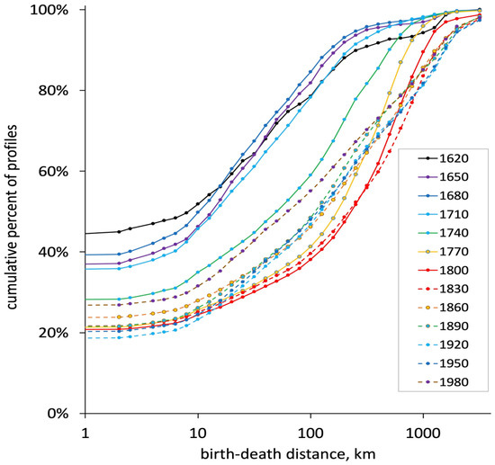
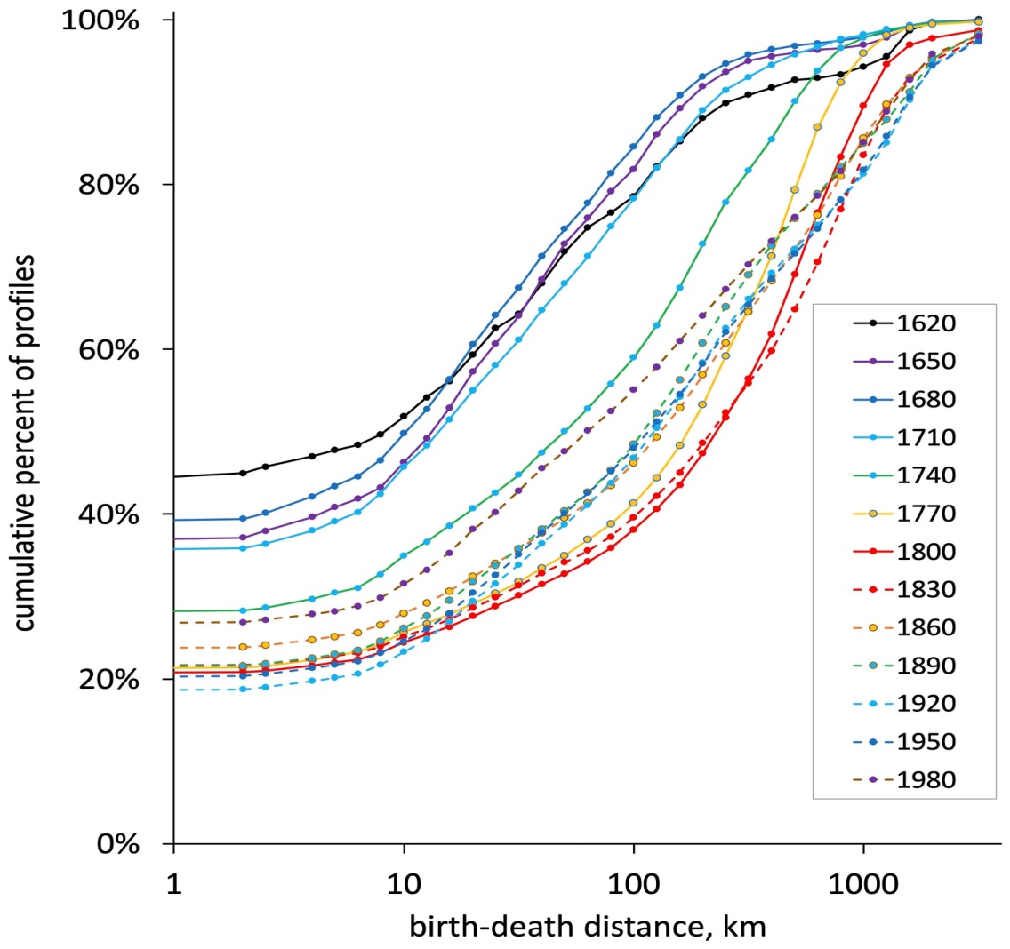
The third and most interesting deviation from the 1/r distribution is not shown in Figure 2; it begins in the US data after 1710, characterized by an order-of-magnitude increase in median migration distance with striking divergence from the power law, as shown in Figure 3.
Figure 3.
Cumulative distributions of 2.83 million North American birth-death distances. Unlike Figure 2, all profiles are counted, including those who did not move, so the percent of “stayers” appears as the vertical axis intercept. Each curve is a 30 year (generational) subset of 20-year-olds; thus, the 1620 data tallies those aged 20 years between 1620 and 1649. In all cases, at least 100 profiles are counted in the smallest distance bin (2–2.5 km) from which counting proceeds in ten bins per factor of ten.
3.4. The Late Colonial American Shift
Figure 3 shows that from 1620 to 1710, the American migration distribution follows the European pattern, but then from 1740 to 1800—in only two generations—there are three dramatic shifts. The left vertical intercept shifts dramatically down as the number staying home drops from 40% to 20%. At the same time, the maximum migration distance (the distance at which the distribution extrapolates to 100% of the population) increases from ca. 200 km to 1000–2000 km. Finally, the clean power law collapses (the linearity of the semilog CDF vanishes) as many people move 50–100 km or more.
From 1860 onward, the distributions return partly to the colonial pattern, though total “leavers” remain in the 70–80% range.
3.5. Three Parameter Model
The 1/r distribution in the European and early American data is so prevalent for so long that it is unlikely that its driving forces suddenly vanished around 1740; it is more likely that a new factor appeared. Fitting the observed distances to a mathematical model can help to separate and quantify the transition.
Two parameters are obvious. Britain and Ireland are geographically smaller than Europe or North America, and the British-Irish distributions plateau at a two-to three-fold lower distance than the others (Figure 2b); thus, one parameter should be a maximum distance, interpretable as a maximum physical or perceived range for migration. The second simple parameter is a fraction comprised of people who move at all (“leavers”) versus those who die very near their birthplace (“stayers”). Even within the colonial era 1620–1710, the percentage of leavers rose from 59% in 1620 to 68% in 1710 (Figure 3). By fitting this value, we avoid arbitrary distance thresholds for stay-vs-leave. The stay-vs-leave fraction is also the historical determinant of city-size distributions (Spencer 2024).
A third parameter is necessary to push the post-colonial US distributions to longer distances for a majority of people (Figure 3, after 1710). The data suggest that this parameter should have units of distance and, because the distributions become short-tailed, that it should take the form of a fixed distance. Decomposing migration cost into a linear combination of a fixed and distance-dependent components, integrating, and normalizing gives a three-parameter model for migration distance (Supplementary Material SM4):
CDF = 1 − fleave(1 − ln(1 + r/rfixed)/ln(1 + rmax/rfixed))
This is an empirical model, useful for decomposing and comparing migration across time and geography. Fits are excellent (Supplementary Materials SM1, SM2, SM4 and SM8) with a rms error ~3%, showing that the principal determinants of migration distance may be captured in three parameters. Comparing thousands of temporally and geographically defined data subsets shows that the three parameters are uncorrelated (Supplementary Material SM5).
Most studies measure migration between administrative areas—counties, states, or countries—as recorded in censuses. This gives rise to a long-standing problem: the diversity of those areas’ geographic and population sizes makes comparisons across time and space difficult or badly biased. Viewing migration distances as a distribution and fitting that distribution to a model, e.g., Equation (1), can reduce and quantify that bias (Supplementary Material SM6).
3.6. Decomposition by Time
With millions of datapoints, we can slice our dataset into fine-grained subsets by time and geography and still have sufficient data per subset to obtain excellent fits to the three-parameter model. Observing the fitted values by time (in charts) and space (in maps) then makes interpretation straightforward.
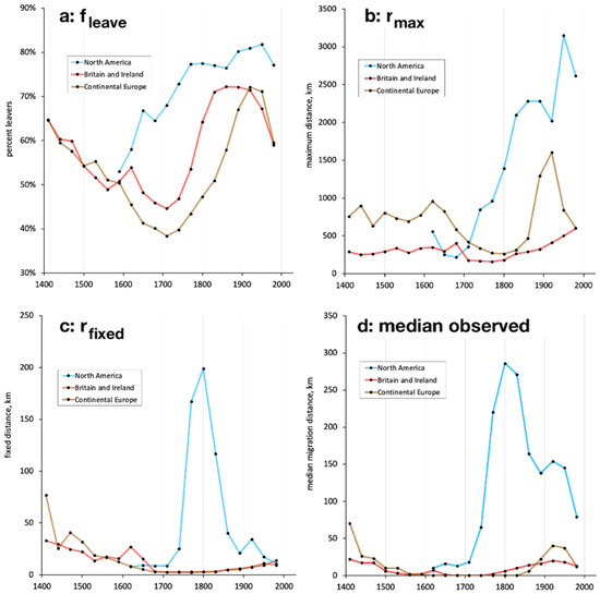
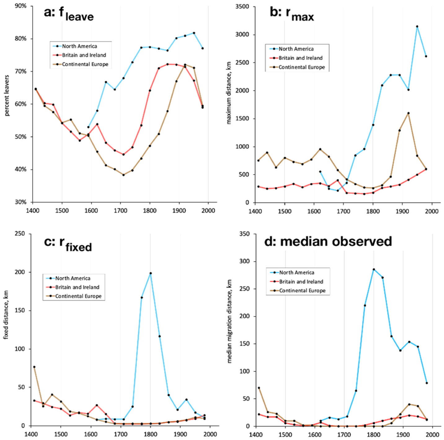
Figure 4 shows how the three parameters change over time on different continents, extending Kaplanis et al.’s observations on median migration distance (Kaplanis et al. 2018, Figures S18 and S19). The percent leaving home (Figure 4a) falls from 65% to 40–50% from medieval to early 18th century Europe, then rises with rural-to-urban migration in the Industrial Revolution for Britain and Ireland and in the 19th century for Continental Europe. Americans’ fleave rises steadily from European values to 80% by 1770, where it plateaus.
Figure 4.
Fitted values for fleave, rmax, and rfixed of Equation (1), and observed median migration distance, by region and 30-year time slice. Each point represents a minimum of 1500 profiles (median 12,900 for Britain and Ireland, 149,700 for North America, and 63,100 for Europe). Mean fit rms errors are 0.9% for Britain and Ireland, 1.3% for North America, and 0.75% for Europe.
The maximum extrapolated distance rmax, Figure 4b, is stable in Europe in 1400–1650, when it curiously falls, only to rise in 1860–1950. This distance is essentially constant for the British Isles in 1400–1980, reflecting the absence of barriers and finite size of these islands. In North America, the rapid rise of rmax parallels the growing awareness of the opportunity (Lewis and Clark return in 1806) and is certainly brought to continental scale by the 1848–1855 Gold Rush that brought 300,000 people to California.
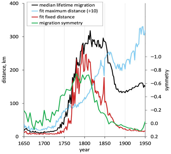
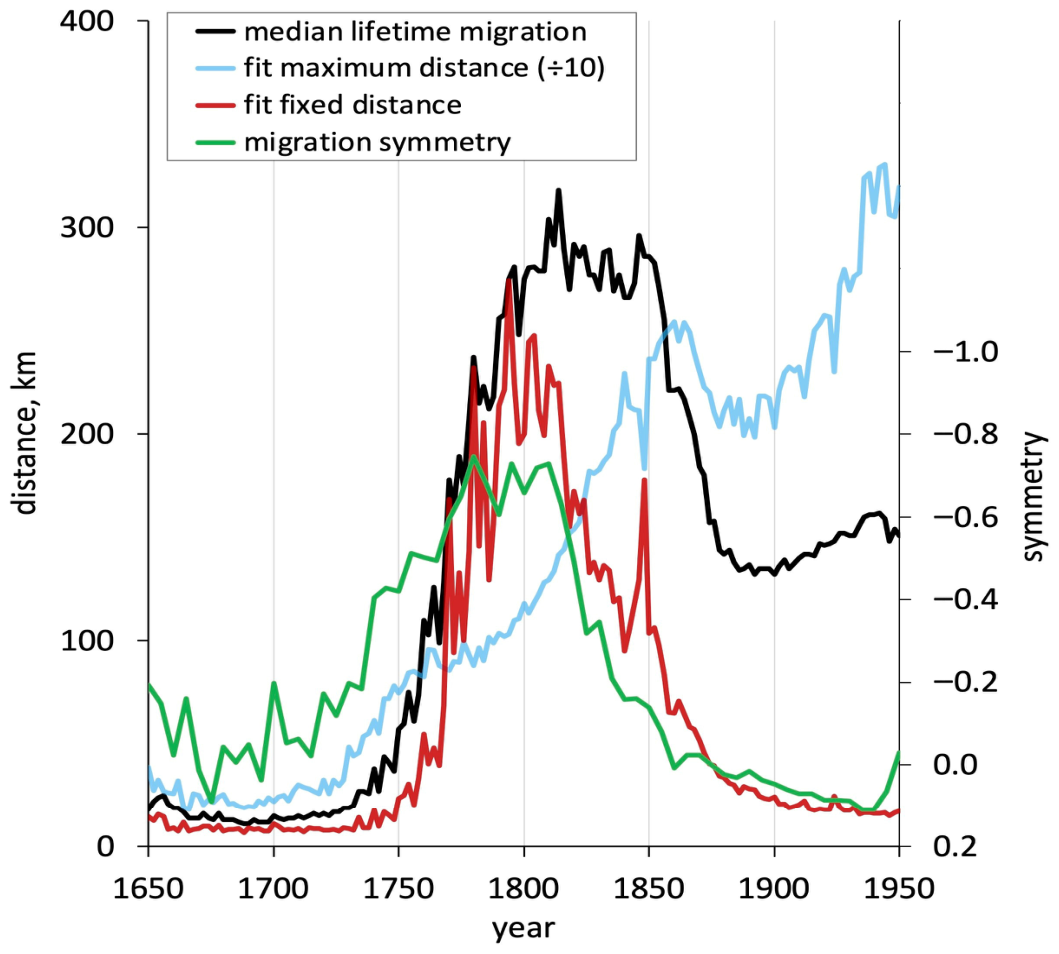
Values for the third fitted parameter rfixed (Figure 4c) are low (0–25 km) and stable in Europe and the British Isles in 1550–1980, and we suggest that this principally represents the distance resolution limit of the Kaplanis data (see Supplementary Material SM7 for a census-based dataset with a known and much greater resolution limit). But the American rfixed displays a unique spike from 1730 to 1890; this cannot be due to a resolution limit because the data source is unchanged, and the magnitude (200 km in 1800) is ten- to twenty-fold higher than the earlier baseline. A fine-grained overlay of this era (Figure 5) emphasizes the independence of rfixed (red) and rmax (blue) and shows that the observed median lifetime migration distance (black) can be decomposed into contributions from both. We will see that this spike in rfixed is a principal distinguishing feature of “frontier” versus “steady-state” migration.
Figure 5.
(Left) axis: American distance parameters over time; 2.67 million profiles total, median 10,800 per 2 year slice. The 1750–1890 spike of rfixed is shown in red, with rmax in blue and measured median birth-death distance in black. (Right) axis: Internal migration symmetry (green) as median of 1° geographic blocks with at least 40 births and deaths per 5 year period.
3.7. Decomposition by Geography
Decomposition by time clarifies some of the determinants of migration distance, such as the leap in British and Irish “leavers” coinciding with the Industrial Revolution noted above. One possible cause for the American spike of rfixed is that economic and technological changes made migration easier and less expensive than it had been, but this cannot account for the return of rfixed to its baseline by 1890. An alternative explanation is suggested by the geographic concentration of high rfixed in western New York state and east of the Appalachians from Virginia to South Carolina (Supplementary Material SM8). These would-be migrants faced a significant barrier (Ontario or Lake Erie or the Appalachian Mountains), but knew that attractive land lay beyond, and so incurred a “fixed cost” to cross that barrier. They were also a decade older when they moved than earlier or later generations (Supplementary Material SM3), suggesting that they needed time to acquire the resources for the longer jump.
Because our dataset records birth and death locations by latitude and longitude, not by county or state, we created and mapped data subsets in geographic blocks, typically 0.5° × 0.5°1. The distributions of profiles in such blocks with the highest and lowest values of rfixed are illustrative (Supplementary Material SM8, lower chart). The lower third, along the New England coast, have the same distribution as the colonies as a whole in 1710—their behavior did not change, and their migrations follow the 1/r distribution. The upper third, in western New York and Virginia to South Carolina, has a short-tailed distribution with a fitted rfixed of 548 ± 32 km (203,000 profiles, rms error 1.8%)—a distance sufficient to cross the Appalachians or Lake Erie.
3.8. Vector Orientation
Up to this point, our research has been a data-driven exploration of what may be learned about migration from genealogic birth-to-death distances. But the observation of a strong anomaly in 1740–1860 in America (Figure 4) suggests a hypothesis, namely, that there is “steady-state” migration (Europe, early American colonies) which differs quantitatively from “frontier” migration (the transient anomaly). We therefore calculate additional metrics—not of distance but of direction and symmetry—to supplement the results.
With genealogic birth and death locations in latitude and longitude, the direction of each life vector is readily calculated. The dominant westward direction of American expansion is apparent (Supplementary Material SM9), in good agreement with the directionality of the largest DNA clusters of Han et al. (2017), Figure 3. The average early colonial vector is southwest (from Boston down the coast) but by 1800–1830 the arc is due west (270°) and remarkably narrow, and then broadens back to colonial variance by 1920–1950. The narrow spread of the angular distribution (Figure 6, green) coincides with the spike in rfixed (red). Thus, the dominance of the western pattern of migration for that century (1800 to 1920) is neatly described.
Figure 6.
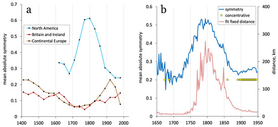
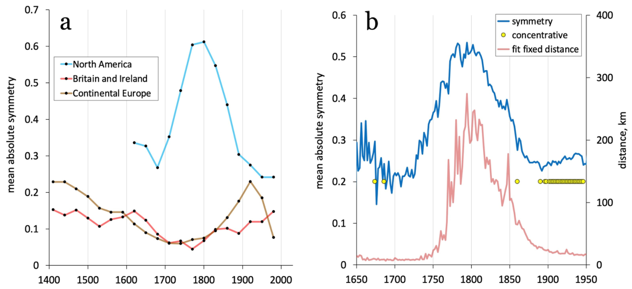
Migration symmetry by region and date. Values are mean absolute symmetry = Σ|S|/n over all 1 × 1° blocks in (a) the indicated region in 30 year time slices and (b) North America in 2 year slices. Panel (b) repeats the data for rfixed of Figure 5 to show their temporal overlap. Yellow dots in (b) indicate time slices for which ΣS is positive, i.e., migration concentrates the population; otherwise ΣS is negative or dispersive.
3.9. Symmetry of Migration
A symmetry metric is also readily found for any given region and time period by counting births and deaths, but only across different regions because we are concerned with migration and not population growth: S = (births − deaths)/(births + deaths) where births = number of genealogic profiles with birth location in the given block but death outside, and deaths = number born outside the given block and who died within.
Migration is at a steady-state when S equals zero; 1 > S > 0 indicates net efflux (more people leave than arrive) and 0 > S > −1 indicates net influx (Supplementary Material SM10). The absolute value of S measures net migration, and the mean of |S| for a large area’s composite blocks (e.g., counties or geographic blocks) is a measure of whether it is near or far from a steady-state. Figure 6 shows Great Britain, Ireland, and Europe in a near-steady-state for the past 600 years. Certainly, there is asymmetric migration in specific times and places, for example, rural Britain to industrial cities after 1750, but overall internal migration is close to reciprocal. Again, North America is quite different with much higher “churn” from the colonial era to the present; it is a system far from a steady-state. Decomposing by geography (maps Supplementary Materials SM10 and SM11) shows that the unique peak of mean absolute symmetry in 1710–1890 is due to migration into essentially empty areas (as far as the settlers were concerned, ignoring Native Americans) that could not be reciprocal. The sign ΣS shows that 1710–1890 migration was dispersive (frontier) and changed to concentrative about 1900 (Figure 6, yellow dots; full distributions Supplementary Material SM10) as internal American migration became dominated by urbanization and moves to warmer climes (Supplementary Material SM10). The recent baseline (1920–1980, S ~ 0.25) remains 2–3-fold above the European norm; America is a dynamic system relatively far from equilibrium.
4. Discussion
We have made several original quantitative observations: that human migration has followed a 1/r distance distribution for centuries, that migration distance can be decomposed into three independent parameters, and that directionality and migration symmetry may be easily calculated from genealogic data. Each of these warrants its own discussion below, after which we synthesize a new quantitative definition of a frontier, which is based on the American frontier but is generally applicable even in prehistory.
4.1. Interpreting the Inverse Distance (1/r) Distribution
Because the data in Figure 2 precede the US frontier era and are taken from a wider geography, their pattern is the backdrop against which the American expansion can be contrasted.
Ancient Roman and early medieval city sizes in Figure 1 challenge technology-based theories of city growth. Figure 2 does the same for migration theories: whatever drives this pattern of human migration cannot depend on post-industrial communication or technology because the distributions before and after 1750 are essentially identical.
Temporal and geographical subsets of the Kaplanis data make it possible to exclude a variety of factors which might give rise to the observed distribution. Firstly, the distribution is not dependent on population growth. From 1550 to 1750, European and British population growth was low, doubling every 360 years, while the American colonial population grew an order of magnitude faster, doubling every 24 years2. Secondly, distributions of internal migration are separable from significant international migration, either as emigrants (from Europe) or immigrants (to North America). Thirdly, the distributions are minimally dependent of gender: the differences between eras and regions greatly exceed the differences between female and male migration (Supplementary Material SM2).
Power-law distributions for travel have been observed before. Zipf’s early rationale was that the optimization of intercity transportation costs, assuming that such costs are proportional to distance (Zipf 1946), led to the observed 1/r dependence, though he measured frequent and reversible travel (train and bus passengers), not lifetime migration, and assumed a constant, steady-state population. Others have observed power laws in travel rationalized by gravity models, radiation models, intervening opportunity models and more (Gonzalez et al. 2008; Levy 2010; Alessandretti et al. 2020; Simini et al. 2012; Schläpfer et al. 2021). This literature finds exponents of either −1 or −2 and, like Zipf’s study, is concerned with a modern era of commuting-scale reversible travel. Most of the models are symmetric with travel flows and proportional to the product of the origin and destination populations—but this is irrelevant to new-settlement scenarios (early colonial America) that are very far from a steady-state with essentially zero population at the destination. Given these contradictions, inapplicability to our medieval-to-modern timescales, empirical disagreement with slope −2 results, and the possible irrelevance of commuting to migration behavior, we eschew these models as well as the premise that human behavior should have commonality with Newtonian masses or radiating particles.
That migration distance (not just travel distance) follows a robust inverse-distance power law is not new, having been documented in the literature from Zipf (1946) to Boucherie et al. (2024). Our contribution is the observation that this pattern has persisted from at least the 16th to the 21st century across two continents (Figure 2), which allows us to say what does not give rise to this pattern. It does not depend on post-industrial communication or transportation. It does not depend, as required by gravity models, on a reciprocal pull from distant population centers. It does not depend on reversible exploration. In addition, it does not depend on population stasis or growth, nor on the gender of the travelers. The origin of the 1/r dependence is uncertain but must be pre-industrial and cross-cultural; it may arise in our innate logarithmic perception of distance and cost (Boucherie et al. 2024; Dehaene 2003) and even be related to similar distributions of other species’ foraging behavior (Gonzalez et al. 2008). What matters here is only that the 1/r distribution of migration distance is a robust observation that can be parameterized, observed across time and geography, and examined for exceptions that illuminate history.
Taking an underlying power law with slope −1 as a given, migration distance can then be decomposed into a model with only three fitted parameters; fitting a wide range of temporal and geographical data subsets shows that the model is widely applicable (root mean square error 2–4%) and the parameters are uncorrelated. The distribution of migration distance retains its 1/r character over the entire observed range of two of the parameters, namely, from 40% to 70% of young adults leaving their birthplace (fleave), and a maximum distance rmax ranging from hundreds to thousands of kilometers. The distribution becomes short-tailed (the power law breaks down; the distance range is narrow) when the fixed-cost term rfixed is well above the intrinsic resolution of the data (ca. 10–20 km, Supplementary Material SM6) which occurs only during the American expansion from 1770 to 1860 (Figure 6) and only in specific locations (Supplementary Material SM8).
4.2. The Decision to Leave, Expressed as fleave
The three parameters of Equation (1) are statistically independent and have independent interpretations. Each illuminates a different aspect of migration.
The conventional wisdom is that American young adults have a greater tendency to leave home than Europeans, though Long and Boertlein (1976) assert that “statistics which permit accurate comparisons among countries in this respect are of very recent origin.” We disagree; genealogies yield quantitative measures that span centuries. Colonial American fleave begins its steep rise from ~50% to 80% almost immediately (Figure 4a). One contributing factor could have been a desire to land-grab before the wilderness was all claimed and parceled. Additionally, the premise of the 1/r distribution is that there is some sort of cost, proportional to distance, associated with leaving home. If the emotional portion of that cost—leaving behind family and the familiar—had already been paid by trans-Atlantic emigration, and/or if settlement was so fast and sparse that cohesive towns had not developed, then there would be weaker ties for colonial young adults, resulting in both a lower barrier to leave home and a reduced cost associated with long distance. Fischer (1989) notes the regional and cultural differences in colonial America, namely, that those in the Southern Highlands were far more likely to move (persistence 25–40%) than New Englanders (75–96%) and had a relaxed approach: “When I get ready to move, I just shut the door, call the dogs, and start.” (Fischer 1989, p. 759). Our data show that from 1740 to 1800 the high propensity to leave was indeed concentrated in Virginia and the Carolinas, but after 1830, 80–90% of young adults leaving home was widespread3.
4.3. Independent Decisions
Because there is clearly a strong distance dependence on migration, could the stay-vs-leave decision be an artifact of the 1/r distribution? That is, are “stayers” simply those whose migration distance falls on the 1/r distribution but is too small to be measured? The 2010 census study is suggestive because the high percentage of stay-at-homes (70%) drops significantly (to 40–50%) if the distance unit is extrapolated from a commuting zone (~80 km) to a town-scale distance (~10 km) (Supplementary Material SM7). However, we believe the two key decisions (stay-vs-leave, how far) to be independent. The modeled parameters are uncorrelated (Supplementary Material SM5). Their timing is uncorrelated: Britain and Ireland in 1740–1830 and North America in 1620–1710 see a large rise in leavers but no meaningful change in distance (Figure 4). The distribution of city sizes across all cultures and eras is consistent with a simple stay-vs-leave parameter independent of distance (Spencer 2024). We suggest that the stay-vs-leave decision is significantly driven by local factors (How many siblings do I have? Can I inherit the farm or business?) while the how-far decision is driven by distance-related factors (Where are the risks and opportunities? Can I rely on anyone there? How will I travel?).
4.4. Maximum Distance, Expressed as rmax
Internal migration has been constrained by geography in Britain and Ireland, and by political boundaries in Europe, for most of recorded history. But in North America, a continuing series of explorations and events (the Great Lakes in the 17th century, Boone’s Wilderness Road in 1775, Lewis and Clark, 1804–1806, and Sutter’s Mill in 1848) increased the maximum migration distance from British scale (~200 km) to continental scale (~2500 km) in four generations (Figure 4b). These limiting distances are consistent, and therefore explain, the observed values of rmax.
4.5. Fixed Distance, Expressed as rfixed
The geographic locations of the 1770–1860 spike in rfixed suggest that this term records a jump over a barrier, essentially a fixed cost that precludes short migration distances and therefore disrupts the 1/r pattern. This interpretation is supported by another large physical barrier encoded in the genealogies, namely, the unavoidable 5000 km trans-Atlantic voyage of European emigrants to North America. We do not include these immigrant profiles in our analysis for several reasons: firstly, transnational migration is well studied so we have focused on internal migration; secondly, these profiles disrupt distance distributions to the point that they are no longer monotonic, and with the additional term(s) or rules required for their modeling there would be no net gain of understanding. These profiles may also be prone to selection bias because the Kaplanis data draws from Geni.com, an American crowd-sourced genealogy site likely to select for immigrant vs. European local migrant profiles. That said, the life-death distances of those born in Ireland in 1790–1850, and therefore alive during the potato famine, show fixed-distance terms consistent with crossing water barriers to Britain, to North America, and to Australia.
A large fixed-cost term would not seem essential to a frontier: it is easy to imagine a large-scale, asymmetric, irreversible, directional movement of people without a major geographic barrier. And yet the best such examples may be prehistoric (see below); perhaps we humans pushed across all of the easy (walkable) routes millennia ago, giving Eurasia time to settle into a steady-state until technology (ocean-crossing ships) broke down those barriers to unleash another frontier in the Americas.
4.6. Symmetry and Directionality
Gravity and related models assume steady-state migration and encode symmetry in their numerators with migration between A and B proportional to (population of A) × (population of B) (Simini et al. 2012, Equation (1); Barbosa et al. 2018, Equation (4)). Strictly speaking, mean absolute symmetry S should be zero under a gravity model, but we can take six centuries of relatively stable British and Irish and European data with 0.5 < S < 0.2 to represent a realistic steady-state for internal migration (Figure 6a). Americans are not just more mobile (Figure 4), they are farther from equilibrium with 0.25 < S < 0.6, a substantial violation of the gravity premise. The spike of S begins about 1740, thirty years before that of rfixed (Figure 6, right). This early phase travels up northern rivers and into central Virginia (Supplementary Materials SM10 and SM11), which is relatively easy geographically and therefore consistent with interpretation of the rfixed spike caused by must-cross barriers.
Horace Greeley’s admonition was well founded: the spikes of rfixed and S coincide precisely with a very narrow due-west distribution of migration direction (Supplementary Material SM9) that reflects a similar directionality toward opportunity and geographic paths.
4.7. Metrics and Properties That Distinguish the Frontier
Our distance, directionality, and symmetry parameters have stable and comparable values for early colonial North America and Europe 1400–1950. We use the term frontier4 to denote places and times when their values are markedly different. Table 1 summarizes the properties of what we call this frontier pattern vs. its steady-state alternative.
Table 1.
Properties that Distinguish Steady-State and Frontier Migration.
4.8. Mapping the American Frontier
It is not our goal to redefine the American frontier, which has been endlessly portrayed in scholarly works, books, films and maps. But given our quantitative temporal and spatial results, we would be remiss not to discuss them in the context of classic maps. Such maps are usually based on population density from census data, typically as the line dividing areas of two or more people per square mile from areas with fewer (Gannett 1903; Otterstrom and Earle 2002; Bazzi et al. 2020). Yet, population density is a metric of convenience: deserts and bodies of water have exceptionally low population densities, but their boundaries would not be considered frontiers because they are inanimate and stable.
A frontier is defined by the movement of people, and arguably ends when people “settle down” and stop moving, for which an appropriate measure is the fraction of those who do not leave their birthplace, i.e., 1 − fleave; a value of 10% staying roughly corresponds to the classic census frontier line (Supplementary Material SM11).
Migration symmetry S may also be used to delimit the frontier. Frontier expansion is just that—expansion— namely, the movement from higher to lower density, therefore requiring ΣS > 0 for regions behind the frontier and ΣS < 0 ahead of it. The S = 0 line is quite a good frontier marker (Supplementary Material SM11). Maps of our symmetry metric have the additional advantage of conveying the frontier’s past and future, where people came from, and where they went.
These two metrics—the fraction staying and migration symmetry—are intrinsically about people moving. They are independent of baseline population growth. Symmetry reverts to a steady-state value after the frontier passes by. These metrics are available from genealogies starting in medieval Europe and 1620 in North America—six generations before we can visualize the frontier with census data. Indeed, it is noteworthy that our measures do not depend on population density to demarcate the frontier line, as other studies have.
4.9. Implications
We refer to the historically dominant (non-frontier) pattern of migration as steady-state. Its power-law distribution reflects a majority of short moves and a few long moves, as evidenced by median migration distances under 50 km (Figure 4d), a distance that can be covered on foot in a few days. Short distances mean that migration can be reversible and need not sunder family and cultural ties. It can be exploratory at first and later to a known destination; in the last two centuries, it is most often city-to-city. We agree with the literature that such migration is driven by personal optimization. As an individual behavior, it has no coordinated common direction. At a true steady-state, such migration must be symmetric, as gravity models demand, and as such is indefinitely sustainable.
Although the American migration distance metrics are quite different from the European baselines (Figure 4), these metrics do not require a frontier by themselves. But their coincidence in time and place with strong asymmetry and directionality—all derived from the same genealogies—assure that these descriptors do, in combination, represent a consistent frontier pattern. Importantly, most of these metrics revert to early colonial or European levels by 1860–1890, signaling the end of the frontier era.
The values of our metrics in the frontier era have strong implications. Median migration distances of 150 to 300 km (Figure 4d and Figure 5) require significant effort and time, making it functionally irreversible (before modern transportation) and breaking family ties. Destinations might be known in general (broad woodland or prairies) but not specifically. There was no one (excluding the indigenous people) at the far end, precluding symmetry. Very narrow directionality (Supplementary Material SM9) implies coordination; people were communicating about opportunities and options and not acting independently (i.e., unlike later urbanization which is largely isotropic). The frontier pattern is not sustainable but self-extinguishing.
By our data-based definition, American frontier migration ends with the return-to-baseline of rfixed, directionality, and symmetry, all during 1860–1890. But two metrics, rmax and fleave, remain high despite frontier closure: the first, because knowledge cannot be unlearned (California is always an option for a New Yorker and vice-versa) and the second, because the coincidental appearance of inexpensive long-distance communication and transportation keeps young adults aware of opportunities while decreasing cultural or family disruption.
4.10. Other Frontier Examples
Our data-driven goal has been to extract patterns from large genealogic datasets, not necessarily to characterize the post-1740 American expansion: that simply happens to be the largest and best-documented element in the data and so provides the clearest context and narrative. With our parameterized definitions (Table 1) we can also examine other times and places.
Every frontier migration is an invasion but not every invasion is a frontier migration. Napoleon’s westward path across Europe and Russia makes the distinction: like frontier migration, it was rapid, highly directional, asymmetric, and of limited duration, but it was not gender-balanced and did not result in significant settlement by the newcomers. It did not have a major irreversible effect on the invaded people as measured by their genealogies or DNA.
Our frontier migration pattern has more in common with mass migration to avoid war or famine: a long jump into the unknown that is irreversible, unidirectional, and of relatively short duration. However, two elements distinguish such avoidance migration from frontier migration. Firstly, motivation differs in that the former is “push”, movement away from something, while the latter is “pull”, movement toward something. Secondly, avoidance migration is not generally into an empty or underdeveloped area, but rather into an accommodating civilization.
More complete parallels to frontier migration may be found in prehistory. DNA analysis convincingly shows that two ancient transitions in Europe—Mesolithic to Neolithic, then Neolithic to Bronze Age—were demic, driven by the movement of people (Haak et al. 2015; Olalde et al. 2018; Brace et al. 2019; Chikhi et al. 2002). These were irreversible, directional, frontier migrations of people into regions of low population and with the advantage of new technologies: domesticated plants and animals from the Near East and Anatolia, and then bronze tools, language, and horses from the steppes. The newcomers substantially (Neolithic) and essentially completely (Bronze Age) replaced the locals. The parallels to the frontier era of North America are striking, including reversion to steady-state behavior once the frontier reached the western ocean boundary (Antonio et al. 2024).
4.11. Avenues for Additional Research
Millions of genealogic profiles show that the distribution of lifetime migration distance persists across centuries. That the pattern is pre-industrial and cross-cultural eliminates a host of modern hypotheses for its root cause. Genealogies also provide directionality and symmetry, which with fitted distance model parameters form a set of quantitative descriptors that characterize migration, and specifically distinguish frontier from steady-state migration. Mapping these metrics against known history raises additional questions and avenues for research beyond what we address here. For example:
- The swift rise of fleave from 45% to 70% in Britain and Ireland in 1700–1830 almost certainly reflects migration for new urban, industrial employment, yet it is not accompanied by any change in rmax or rfixed (Figure 4). A similar rise of fleave from 40% to 70% occurs in Europe in 1700–1900, but with (1860–1900) a five-fold increase in rmax. Is this also about urban employment, perhaps to less dispersed locations, or does it reflect political changes (war)?
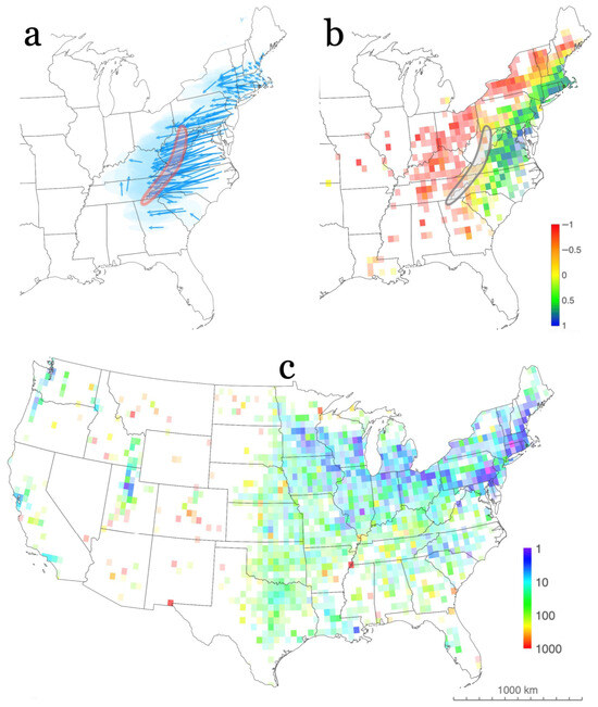
- The location and timing of the 80–90% leavers and >100 km rfixed long-jumpers we see in 1740–1800 in Virginia suggest that this is the Scotch-Irish folkway (Fischer 1989) which begat the stereotypic Appalachian culture. Yet the majority did not stop in the mountains but traveled farther and continued westward (Figure 7a,b). What are the details of these different endpoints from a common origin?
- From 1860–1920 there is a strong arc from Boston, across northern Ohio, into Minnesota, of exceptionally low rfixed, i.e., nearly perfect 1/r distributions (Figure 7c). Most leave home (70–90%) yet travel only 10–30 km. Why does this narrow upper Midwest arc have the same pattern as coastal New England, and differ from that south of mid-Ohio?
- We have considered migrating people as disconnected individuals. Yet even though the Kaplanis data is anonymous (without names or identifiers), profiles include parent-child links via ID numbers, so that chain migration questions can be addressed. For example, are there any correlations between a parent’s stay-vs-leave or migration distance decisions and those of their children? Are children from larger families more likely to migrate? Are there geographic or temporal patterns in family behavior?
Figure 7.
Maps are computed for 0.5° × 0.5° blocks with at least 100 profiles. (a) Median birth-death vectors, tally year 1770; light blue ellipses are ±1 standard deviation of the death locations of those born in the block at the arrow’s origin. Note that the majority of the Virginia-origin vectors cross the Appalachian Mountains (oval shape). (b) Values of symmetry S for 1770 also showing that the majority of this generation dies well west of the mountains (red squares, S ≈ −1, thus the earliest arrivals). (c) Values of rfixed for 1920. Note the blue arc from the New England coast, across Pennsylvania, Ohio, and Michigan, up to Minnesota. Most of these people leave home (fleave = 0.7–0.9) but migrate short distances (median < 30 km) with no fixed-cost penalty (rfixed < 10 km). These and more maps may be found at https://scaledinnovation.com/gg/migration/migration.html (accessed on 11 January 2026).
The power of massive crowd-sourced genealogies can be harnessed to address these and other questions. In particular, the anonymous profiles of the Kaplanis dataset can be matched by time and place, and in some cases exactly by tree matching, to detailed profiles in FamilySearch and WikiTree. Those additional names, life stories, and historic connections can bring this history to life.
5. Conclusions
The birth and death data in genealogic profiles extend migration distance studies from medieval to modern times, and at a temporal and spatial granularity that enables detailed analysis of distributions and correlations. We found two strong patterns in a collection of 86 million profiles. Firstly, steady-state migration, which is universal, symmetric, sustainable, and follows a 1/r distribution of distance. A second pattern appears in North America after 1740, which is longer distance (not power law), asymmetric, directional, and self-extinguishing. Both are quantitatively characterized by a three-parameter distance model plus directional and symmetry terms. The second pattern’s coincidence with American westward migration allows us to reinterpret frontier migration in quantitative terms and offers new insights into American history as well as parallels in ancient Eurasian history. We anticipate that our findings will help explain the spatial order of other migration patterns in different times and disparate parts of the world as they are illuminated within genealogic databases or other large-scale demographic compilations.
Supplementary Materials
The following supporting information can be downloaded at: https://www.mdpi.com/article/10.3390/socsci15050317/s1, SM1: Validation of Genealogic Data; SM2: Dependence on Gender; SM3: Age at Migration; SM4: Three-Parameter Model; SM5: Model Parameter Independence; SM6: Standardizing Migration Data; SM7: 2010 US Census Migration Data; SM8: Geographic Dependence of the Fixed Distance Parameter; SM9: Directionality of American Migration; SM10: Migration Symmetry; SM11: Alternative Frontier Mappings.
Author Contributions
Conceptualization, R.W.S. and S.M.O.; methodology R.W.S.; software, R.W.S.; validation, R.W.S.; formal analysis, R.W.S.; investigation, R.W.S. and S.M.O.; resources, S.M.O.; data curation, R.W.S.; writing—original draft preparation, R.W.S.; writing—review and editing, S.M.O. and R.W.S.; visualization, R.W.S.; supervision, S.M.O.; project administration, S.M.O. All authors have read and agreed to the published version of the manuscript.
Funding
This research received no external funding.
Institutional Review Board Statement
Not applicable.
Informed Consent Statement
Not applicable.
Data Availability Statement
All source code, maps, and links to primary data sources may be found at https://scaledinnovation.com/gg/migration/migration.html (accessed on 11 January 2026). The data of Kaplanis et al. 2018 is at the mirror site https://osf.io/fd25c/overview (accessed on 11 January 2026).
Conflicts of Interest
The authors declare no conflict of interest.
Notes
| 1 | At 37 °N a 0.5° × 0.5° block has dimensions of 44 × 56 km = 2500 km2. In the lower 48 states there are 3108 counties with mean area 2600 km2. In effect these blocks are near constant-area counties. |
| 2 | Growth rates are readily calculated from population data, e.g., https://en.wikipedia.org/wiki/Demographic_history_of_the_United_States (accessed on 11 January 2026). |
| 3 | See https://scaledinnovation.com/gg/migration/migration.html?type=fleave&loop (accessed on 11 January 2026). |
| 4 | We acknowledge that what can be called frontier migration from one side can be called an invasion from the other. Our story is necessarily one-sided due of the availability of genealogic data. No bias or judgment is intended. |
References
- Abel, Guy J. 2013. Estimating global migration flow tables using place of birth data. Demographic Research 28: 505–46. [Google Scholar] [CrossRef] [Scilit]
- Abel, Guy J., and Joel E. Cohen. 2019. Bilateral international migration flow estimates for 200 countries. Nature Scientific Data 6: 82. [Google Scholar] [CrossRef] [Scilit]
- Abel, Guy J., and Joel E. Cohen. 2022. Bilateral international migration flow estimates updated and refined by sex. Nature Scientific Data 9: 173. [Google Scholar] [CrossRef] [Scilit] [PubMed]
- Abel, Guy J., and Nikola Sander. 2014. Quantifying global international migration flows. Science 343: 1520–1522. [Google Scholar] [CrossRef] [Scilit] [PubMed]
- Abramitzky, Ran, Leah Platt Boustan, Harriet M. Brookes Gray, Katherine Eriksson, Santiago Pérez, Hannah M. Postel, Myera Rashid, and Noah Simon. 2025. Finding John Smith: Using Extra Information for Historical Record Linkage. No. w33999. Washington, DC: National Bureau of Economic Research. [Google Scholar]
- Adams, John W., Alice B. Kasakoff, and Jan Kok. 2002. Migration over the life course in nineteenth-century Netherlands and the American North: A comparative analysis based on genealogies and population registers. Annales de Démographie Historique 2: 5–27. [Google Scholar] [CrossRef] [Scilit] [PubMed]
- Alessandretti, Laura, Ulf Aslak, and Sune Lehmann. 2020. The scales of human mobility. Nature 587: 402–7. [Google Scholar] [CrossRef] [Scilit]
- Anderson, Margo, and Stephen E. Fienberg. 1997. Who Counts? The politics of censustaking. Society 34: 19–26. [Google Scholar] [CrossRef] [Scilit]
- Anderson, Margo J. 1988. The American Census: A Social History. New Haven: Yale University Press. [Google Scholar]
- Anderson, Margo J. 2019. The Ghosts of Census Past and Their Relevance for 2020. Proceedings of the American Philosophical Society 163: 227–38. [Google Scholar] [CrossRef] [Scilit]
- Antonio, Maria L., Clemens L. Weiß, Ziyue Gao, Stephanie Sawyer, Verena Oberreiter, Hannah M. Moots, Jeffrey P Spence, Olivia Cheronet, Brina Zagorc, Elisa Praxmarer, and et al. 2024. Stable population structure in Europe since the Iron Age, despite high mobility. eLife 13: e79714. [Google Scholar] [CrossRef]
- Arreola, Daniel D., and Rio Hartwell. 2014. Phoenix Population Origins, 1870–1900. Geographical Review 104: 439–58. [Google Scholar] [CrossRef] [Scilit]
- Auerbach, Felix. 1913. Das Gesetz der Bevölkerungskonzentration [The law of population concentration]. Petermanns Geographische Mitteilungen 59: 74–76. [Google Scholar]
- Barbosa, Hugo, Marc Barthelemy, Gourab Ghoshal, Christopher R. James, Maxime Lenormand, Thomas Louail, Ronaldo Menezes, José J. Ramasco, Filippo Simini, and Marcello Tomasini. 2018. Human mobility: Models and applications. Physics Reports 734: 1–74. [Google Scholar] [CrossRef] [Scilit]
- Batty, Michael. 2013. A theory of city size. Science 340: 1418–19. [Google Scholar] [CrossRef] [Scilit] [PubMed]
- Bazzi, Samuel, Martin Fiszbein, and Mesay Gebresilasse. 2020. Frontier culture: The roots and persistence of “rugged individualism” in the United States. Econometrica 88: 2329–68. [Google Scholar] [CrossRef] [Scilit]
- Blazquez, David, and Josep Domenech. 2018. Big data sources and methods for social and economic analyses. Technological Forecasting and Social Change 130: 99–113. [Google Scholar] [CrossRef] [Scilit]
- Boucherie, Louis, Benjamin F. Maier, and Sune Lehmann. 2024. Decomposing geographical and universal aspects of human mobility. arXiv arXiv:2405.08746. [Google Scholar] [CrossRef] [Scilit]
- Brace, Selina, Yoan Diekmann, Thomas J. Booth, Lucy van Dorp, Zuzana Faltyskova, Nick Rohland, Swapan Mallick, Iñigo Olalde, Matthew Ferry, Megan Michel, and et al. 2019. Ancient genomes indicate population replacement in Early Neolithic Britain. Nature Ecology & Evolution 3: 765–71. [Google Scholar] [CrossRef] [Scilit] [PubMed]
- Buckles, Kasey, Joseph Price Adrian Haws, and Haley E. B. Wilbert. 2023. Breakthroughs in Historical Record Linking Using Genealogy Data: The Census Tree Project. No. w31671. Washington, DC: National Bureau of Economic Research. [Google Scholar]
- Chikhi, Lounès, Richard A. Nichols, Guido Barbujani, and Mark A. Beaumont. 2002. Y genetic data support the Neolithic demic diffusion model. Proceedings of the National Academy of Sciences USA 99: 11008–13. [Google Scholar] [CrossRef] [Scilit] [PubMed]
- Chong, Matthew, Diego Alburez-Gutierrez, Enrico Del Fava, Michael Alexander, and Emilio Zagheni. 2022. Correcting Historical Mortality Rate Bias in Big Crowd-Sourced Online Genealogies. Working Paper. Rostock: Max Planck Institute for Demographic Research. [Google Scholar] [CrossRef] [Scilit]
- Chudacoff, Howard P. 1973. A new look at ethnic neighborhoods: Residential dispersion and the concept of visibility in a medium-sized city. The Journal of American History 60: 76–93. [Google Scholar] [CrossRef] [Scilit]
- Chudacoff, Howard P. 2014. New Branches on the Tree: Household Structure in Early Stages of the Family Cycle in Worcester, Massachusetts, 1860–1880. In Institutional Life. Edited by Neil Shumsky. New York: Routledge, pp. 1–18. [Google Scholar]
- Colasurdo, Andrea, and Roberto Omenti. 2024. Using Online Genealogical Data for Demographic Research: An Empirical Examination of the FamiLinx Database. Working Paper No. 62yxm. Charlottesville: Center for Open Science. [Google Scholar] [CrossRef] [Scilit]
- Conzen, Kathleen Neils. 1979. Immigrants, immigrant neighborhoods, and ethnic identity: Historical issues. The Journal of American History 66: 603–15. [Google Scholar] [CrossRef] [Scilit]
- Conzen, Kathleen Neils. 1981. Community studies, urban history, and American local history. In The Past Before Us. Edited by Michael Kammen. Ithaca: Cornell University Press, pp. 270–91. [Google Scholar]
- Dehaene, Stanislas. 2003. The neural basis of the Weber–Fechner law: A logarithmic mental number line. Trends in Cognitive Sciences 7: 145–47. [Google Scholar] [CrossRef] [Scilit]
- Deville, Pierre, Catherine Linard, Samuel Martin, Marius Gilbert, Forrest R. Stevens, Andrew E. Gaughan, Vincent D. Blondel, and Andrew J. Tatem. 2014. Dynamic population mapping using mobile phone data. Proceedings of the National Academy of Sciences USA 111: 15888–93. [Google Scholar] [CrossRef] [Scilit]
- Duzett, Neil, Tammy Hepps, Allen Otterstrom, and Joseph Price. 2025. Detecting Fake People in Historical Records. Social Science History 50: 224–241. [Google Scholar] [CrossRef] [Scilit]
- Fischer, David Hackett. 1989. Albion’s Seed: Four British Folkways in America. America: A Cultural History. New York: Oxford University Press, vol. 1. [Google Scholar]
- Gabaix, Xavier, and Yannis M. Ioannides. 2004. The evolution of city size distributions. In Handbook of Regional and Urban Economics. Edited by J. Vernon Henderson and Jacques-François Thisse. Amsterdam: Elsevier, vol. 4, pp. 2341–78. [Google Scholar] [CrossRef] [Scilit]
- Gannett, Henry, ed. 1903. Twelfth Census of the United States, Taken in the Year 1900: Statistical Atlas; Washington, DC: United States Census Office.
- Gonzalez, Marta C., Cesar A. Hidalgo, and Albert-László Barabási. 2008. Understanding individual human mobility patterns. Nature 453: 779–82. [Google Scholar] [CrossRef] [Scilit] [PubMed]
- Haak, Wolfgang, Iosif Lazaridis, Nick Patterson, Nadin Rohland, Swapan Mallick, Bastien Llamas, Guido Brandt, Susanne Nordenfelt, Eadaoin Harney, Kristin Stewardson, and et al. 2015. Massive migration from the steppe was a source for Indo-European languages in Europe. Nature 522: 207–11. [Google Scholar] [CrossRef] [Scilit] [PubMed]
- Han, Eunjung, Peter Carbonetto, Ryan E. Curtis, Yun Wang, Jennifer M. Granka, James Byrnes, Keith Noto, Amir R. Kermany, Natalie M. Myres, Mathew J. Barber, and et al. 2017. Clustering of 770,000 genomes reveals post-colonial population structure of North America. Nature Communications 8: 14238. [Google Scholar] [CrossRef] [Scilit]
- Hershberg, Theodore, Alan Burstein, and Robert Dockhorn. 1976. Record linkage. Historical Methods Newsletter 9: 137–63. [Google Scholar] [CrossRef] [Scilit]
- Hinde, Andrew. 2004. The use of nineteenth-century census data to investigate local migration. Local Population Studies 73: 8–28. [Google Scholar]
- Hornsby, Stephen J. 1992. Patterns of Scottish emigration to Canada, 1750–1870. Journal of Historical Geography 18: 397–416. [Google Scholar] [CrossRef] [Scilit]
- Hudson, John C. 1988. North American origins of middlewestern frontier populations. Annals of the Association of American Geographers 78: 395–413. [Google Scholar] [CrossRef] [Scilit]
- Hudson, John C. 2024. The Middle West as a Study in Migration. Middle West Review 11: 49–58. [Google Scholar] [CrossRef] [Scilit]
- Kaplanis, Jason, Assaf Gordon, Tal Shor, Omer Weissbrod, Dan Geiger, Mikkel Wahl, Michael Gershovits, Barak Markus, Mona Sheikh, Melissa Gymrek, and et al. 2018. Quantitative analysis of population-scale family trees with millions of relatives. Science 360: 171–75. [Google Scholar] [CrossRef] [Scilit] [PubMed]
- Knights, Peter R. 1971. The Plain People of Boston, 1830–1860: A Study in City Growth. New York: Oxford University Press. [Google Scholar]
- Knights, Peter R. 1991a. Potholes in the road of improvement? Estimating census underenumeration by longitudinal tracing: US censuses, 1850–1880. Social Science History 15: 517–26. [Google Scholar]
- Knights, Peter R. 1991b. Yankee Destinies: The Lives of Ordinary Nineteenth-Century Bostonians. Chapel Hill: University of North Carolina Press. [Google Scholar]
- Koylu, Caglar, Alice B. Kasakoff, and Maryam Torkashvand. 2025. US migration from 1850 to 1920: A comparison of family trees with linked census data. Historical Methods: A Journal of Quantitative and Interdisciplinary History 58: 160–74. [Google Scholar] [CrossRef] [Scilit]
- Koylu, Caglar, and Alice Kasakoff. 2022. Measuring and mapping long-term changes in migration flows using population-scale family tree data. Cartography and Geographic Information Science 49: 154–70. [Google Scholar] [CrossRef] [Scilit]
- Koylu, Caglar, Diansheng Guo, Alice Kasakoff, and John W. Adams. 2014. Mapping family connectedness across space and time. Cartography and Geographic Information Science 41: 14–26. [Google Scholar] [CrossRef] [Scilit]
- Koylu, Caglar, Diansheng Guo, Yuan Huang, Alice Kasakoff, and Jack Grieve. 2020. Connecting Family Trees to Construct a Population-Scale and Longitudinal Geo-Social Network for the U.S. International Journal of Geographical Information Science 35: 2380–423. [Google Scholar] [CrossRef] [Scilit]
- Levy, Moshe. 2010. Scale-free human migration and the geography of social networks. Physica A: Statistical Mechanics and Its Applications 389: 4913–17. [Google Scholar] [CrossRef] [Scilit]
- Long, Larry H., and Celia G. Boertlein. 1976. The Geographical Mobility of Americans: An International Comparison; Washington, DC: U.S. Department of Commerce, Bureau of the Census.
- Markoff, John, and Gilbert Shapiro. 1973. The linkage of data describing overlapping geographical units. Historical Methods Newsletter 7: 34–46. [Google Scholar] [CrossRef] [Scilit]
- Mineau, Geraldine P., Lee L. Bean, and Douglas L. Anderton. 1989. Description and evaluation of linkage of the 1880 census to family genealogies: Implications for Utah fertility research. Historical Methods: A Journal of Quantitative and Interdisciplinary History 22: 144–57. [Google Scholar] [CrossRef] [Scilit]
- Olalde, Iñigo, Selina Brace, Morten E. Allentoft, Ian Armit, Kristian Kristiansen, Thomas Booth, Nadin Rohland, Swapan Mallick, Anna Szécsényi-Nagy, Alissa Mittnik, and et al. 2018. The Beaker phenomenon and the genomic transformation of northwest Europe. Nature 555: 190–96. [Google Scholar] [CrossRef] [Scilit]
- Otterstrom, Samuel M., and Brian E. Bunker. 2013. Genealogy, migration, and the intertwined geographies of personal pasts. Annals of the Association of American Geographers 103: 544–69. [Google Scholar] [CrossRef] [Scilit]
- Otterstrom, Samuel M., and Carville Earle. 2002. The settlement of the United States from 1790 to 1990: Divergent rates of growth and the end of the frontier. Journal of Interdisciplinary History 33: 59–85. [Google Scholar] [CrossRef] [Scilit]
- Otterstrom, Samuel M., Joseph P. Price, and Jacob Van Leeuwen. 2022. Using linked census records to study shrinking cities in the United States from 1900 to 1940. The Professional Geographer 74: 88–101. [Google Scholar] [CrossRef] [Scilit]
- Pouyez, Christian, Raymond Roy, and Francois Martin. 1983. The linkage of census name data: Problems and procedures. The Journal of Interdisciplinary History 14: 129–52. [Google Scholar] [CrossRef] [Scilit] [PubMed]
- Price, Joseph, Kasey Buckles, Jacob Van Leeuwen, and Isaac Riley. 2021. Combining family history and machine learning to link historical records: The Census Tree data set. Explorations in Economic History 80: 101391. [Google Scholar] [CrossRef] [Scilit]
- Ravenstein, Ernst Georg. 1885. The laws of migration. Journal of the Statistical Society of London 48: 167–235. [Google Scholar] [CrossRef] [Scilit]
- Rogers, Andrei, and Luis J. Castro. 1981. Model Migration Schedules. Research Report RR-81-30. Laxenburg: International Institute for Applied Systems Analysis. [Google Scholar]
- Ruggles, Steven, Catherine A. Fitch, and Evan Roberts. 2018. Historical census record linkage. Annual Review of Sociology 44: 19–37. [Google Scholar] [CrossRef] [Scilit]
- Schläpfer, Markus, Lin Dong, Kevin O’Keeffe, Paolo Santi, Michael Szell, Hannes Salat, Samuel Anklesaria, Mohammad Vazifeh, Carlo Ratti, and Geoffrey B. West. 2021. The universal visitation law of human mobility. Nature 593: 522–27. [Google Scholar] [CrossRef] [Scilit]
- Simini, Filippo, Marta C. González, Amos Maritan, and Albert-László Barabási. 2012. A universal model for mobility and migration patterns. Nature 484: 96–100. [Google Scholar] [CrossRef] [Scilit]
- Spencer, Robin W. 2024. City size distributions are driven by each generation’s stay-vs-leave decision. arXiv arXiv:2405.02129. [Google Scholar] [CrossRef] [Scilit]
- Sprung-Keyser, Benjamin, Nathaniel Hendren, and Stephen Porter. 2022. The Radius of Economic Opportunity: Evidence from Migration and Local Labor Markets; Washington, DC: U.S. Census Bureau, Center for Economic Studies.
- Steckel, Richard H. 1988. Census matching and migration: A research strategy. Historical Methods: A Journal of Quantitative and Interdisciplinary History 21: 52–60. [Google Scholar] [CrossRef] [Scilit]
- Stelter, Rebecca, and Diego Alburez-Gutierrez. 2022. Representativeness is crucial for inferring demographic processes from online genealogies: Evidence from lifespan dynamics. Proceedings of the National Academy of Sciences USA 119: e2120455119. [Google Scholar] [CrossRef] [Scilit]
- Swierenga, Robert P. 1989. The settlement of the old northwest: Ethnic pluralism in a featureless plain. Journal of the Early Republic 9: 73–105. [Google Scholar] [CrossRef] [Scilit]
- Thernstrom, Stephan. 1973. The Other Bostonians: Poverty and Progress in the American Metropolis, 1880–1970. Cambridge: Harvard University Press. [Google Scholar]
- Thernstrom, Stephan, and Peter R. Knights. 1970. Men in motion: Some data and speculations about urban population mobility in nineteenth-century America. The Journal of Interdisciplinary History 1: 7–35. [Google Scholar] [CrossRef] [Scilit]
- Ueda, Reed. 2017. Pushing the Atlantic Envelope: Interoceanic Perspectives on Atlantic History. In The Atlantic in Global History, 2nd ed. Edited by Jorge Canizares-Esguerra and Erik R. Seeman. New York: Routledge, pp. 170–83. [Google Scholar]
- Ward, Zachary, Kasey Buckles, and Joseph Price. 2025. Like Great-Grandparent, Like Great-Grandchild? Multigenerational Mobility in American History. No. w33923. Washington, DC: National Bureau of Economic Research. [Google Scholar]
- Waters, Mary C., Reed Ueda, and Helen B. Marrow, eds. 2007. The New Americans: A Guide to Immigration Since 1965. Cambridge: Harvard University Press. [Google Scholar]
- Winchester, Ian. 1970. The linkage of historical records by man and computer: Techniques and problems. The Journal of Interdisciplinary History 1: 107–24. [Google Scholar] [CrossRef] [Scilit] [PubMed]
- Zipf, George. 1946. The P 1 P 2/D hypothesis: On the intercity movement of persons. American Sociological Review 11: 677–86. [Google Scholar] [CrossRef] [Scilit]

Disclaimer/Publisher’s Note: The statements, opinions and data contained in all publications are solely those of the individual author(s) and contributor(s) and not of MDPI and/or the editor(s). MDPI and/or the editor(s) disclaim responsibility for any injury to people or property resulting from any ideas, methods, instructions or products referred to in the content. |
© 2026 by the authors. Licensee MDPI, Basel, Switzerland. This article is an open access article distributed under the terms and conditions of the Creative Commons Attribution (CC BY) license.