
Hourly Calculation Method of Air Source Heat Pump Behavior

 ,
, 
Abstract
:1. Introduction
2. Simulation and Experiment
2.1. Heat Pumps
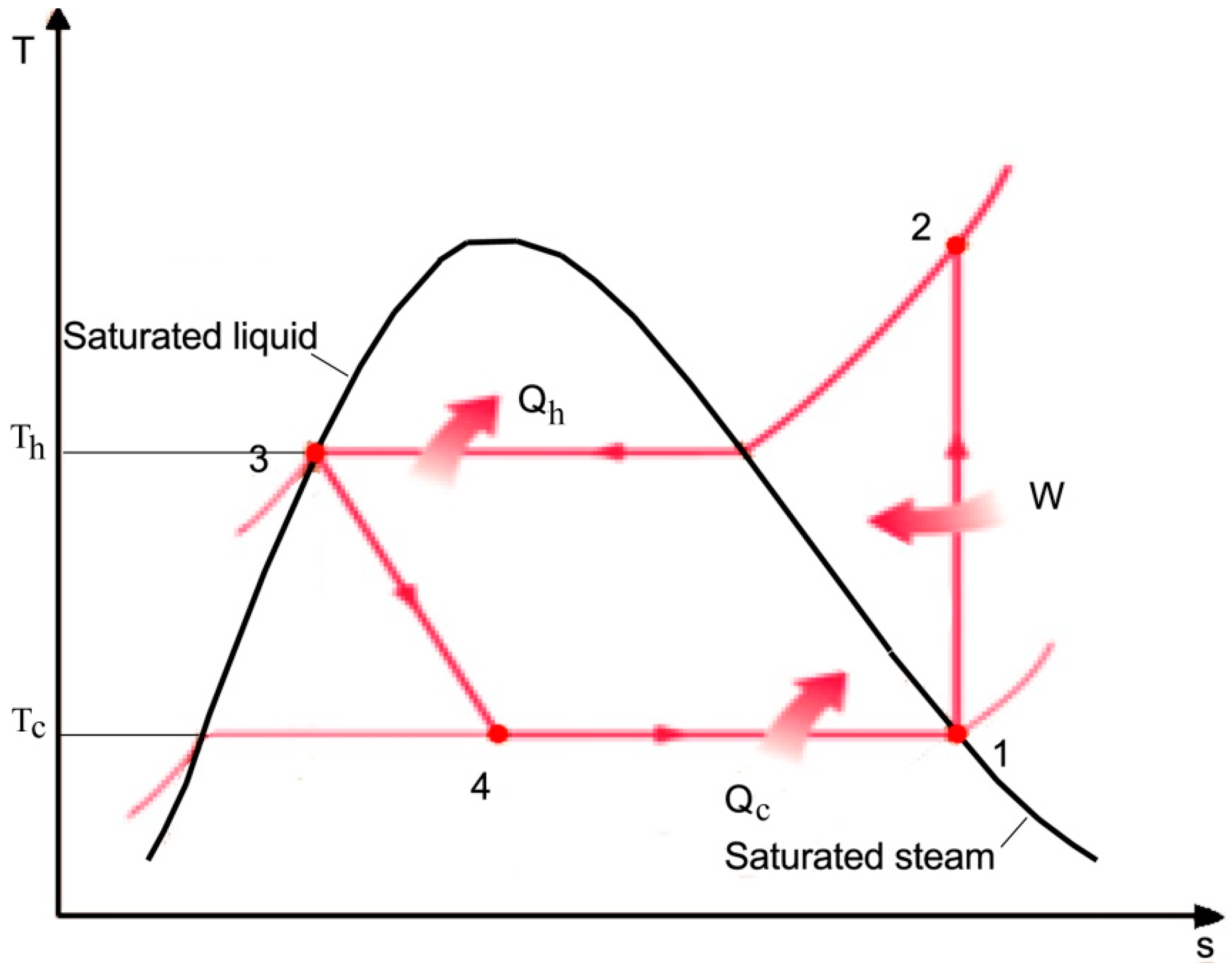
- Tc is the absolute temperature of the cold reservoir (K),
- Th is the absolute temperature of the hot reservoir (K).
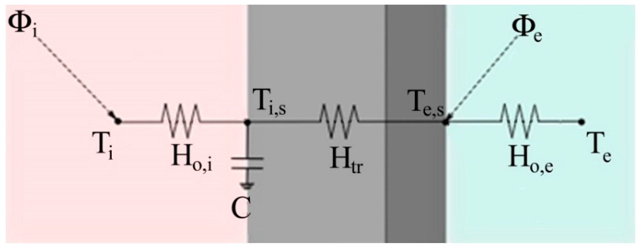
2.2. Calculation Model
- QH,nd is the energy need of the building envelope,
- q is the mass flow rate of the cooling fluid.
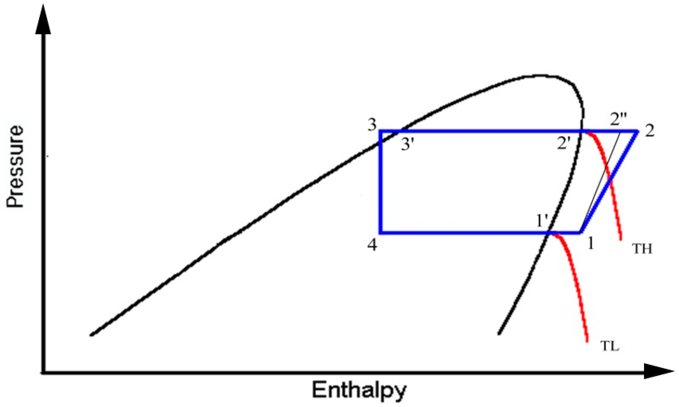
- Wid is the ideal work of compression process;
- Wr is the real work of compression process;
- h2’’ is the specific enthalpy of refrigerant obtained at the end of ideal compression process;
- h1 is the specific enthalpy of refrigerant obtained at the beginning of compression process;
- h2 is the specific enthalpy of refrigerant obtained at the end of real compression process.
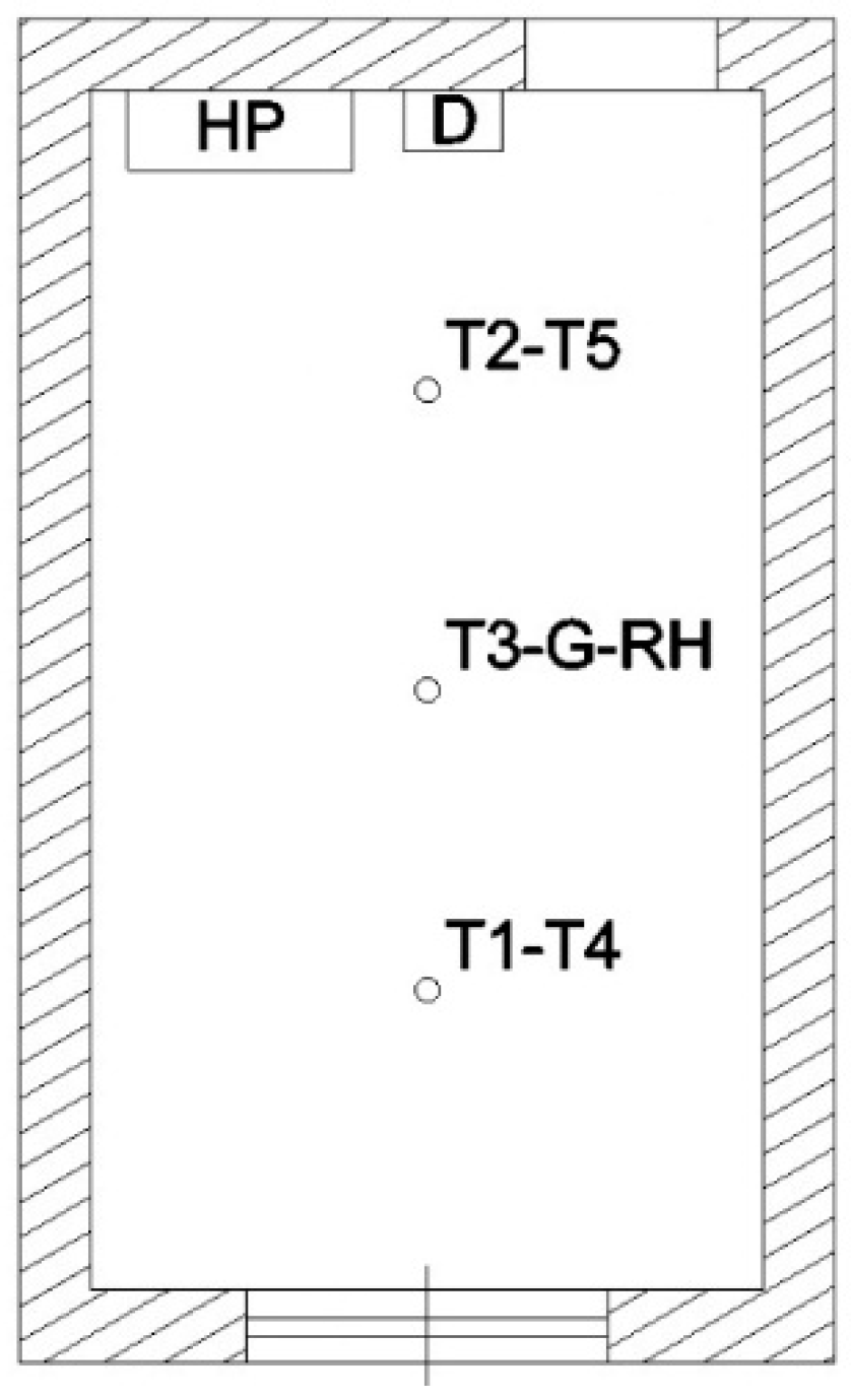
2.3. Test Case
3. Results
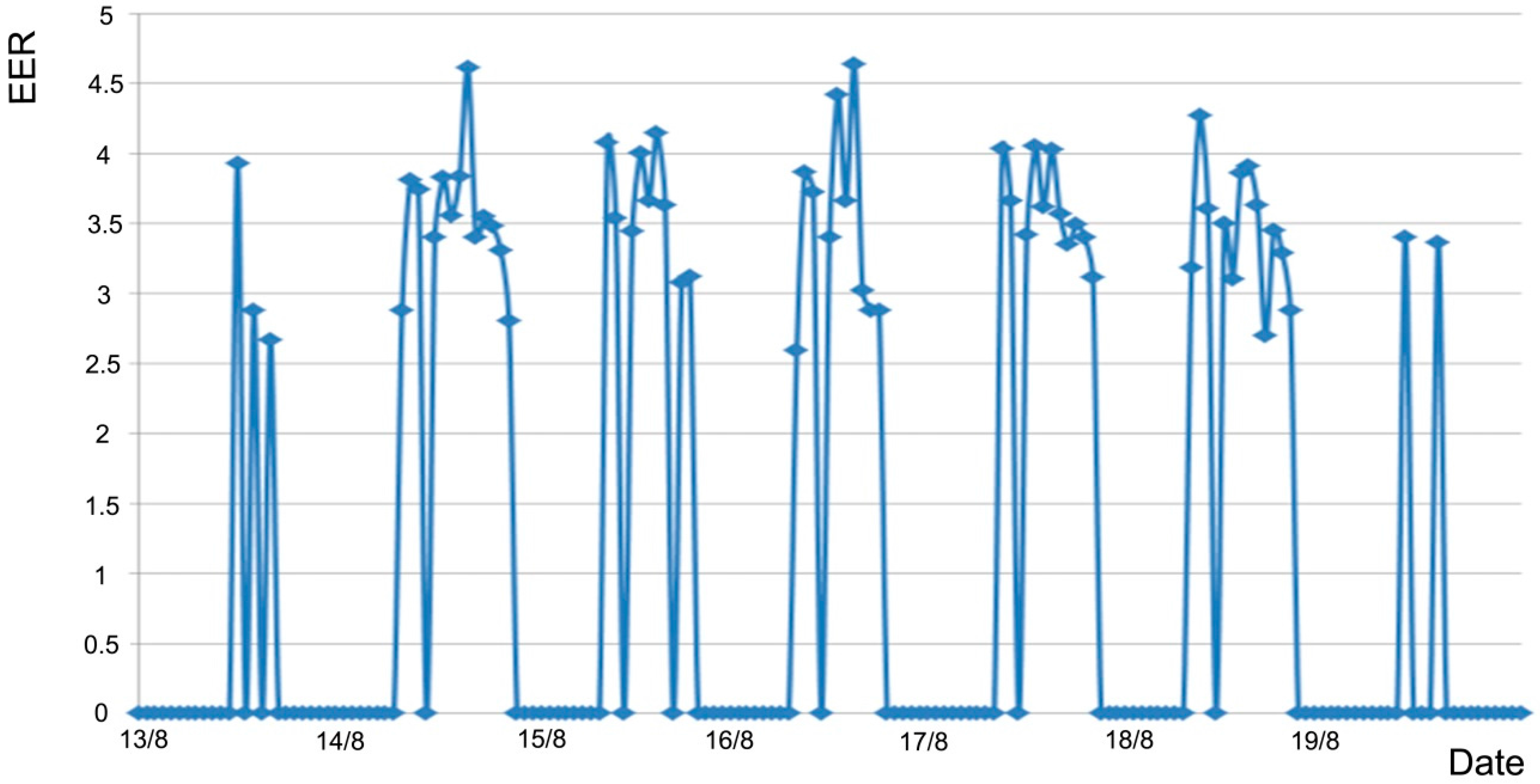
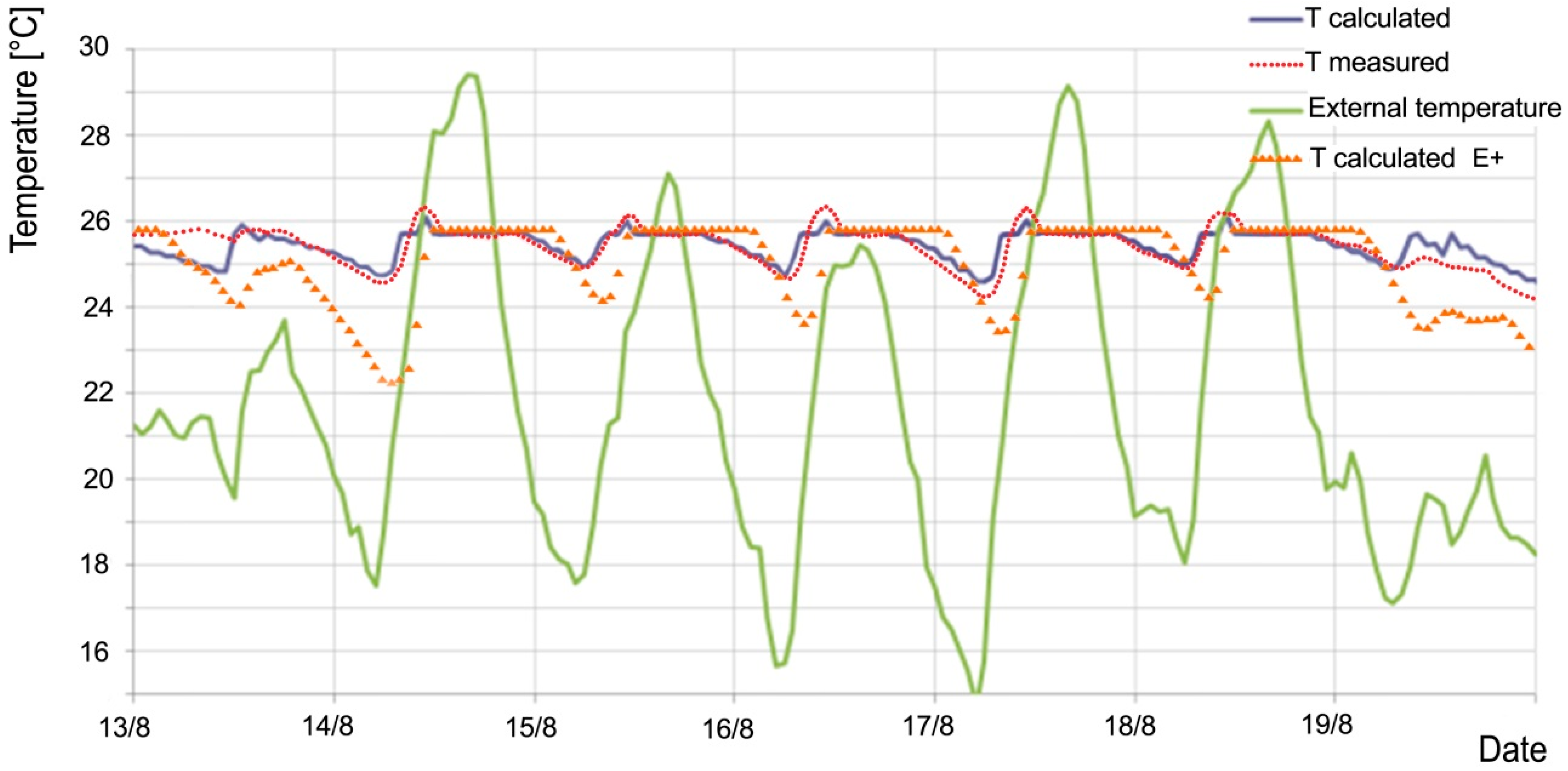
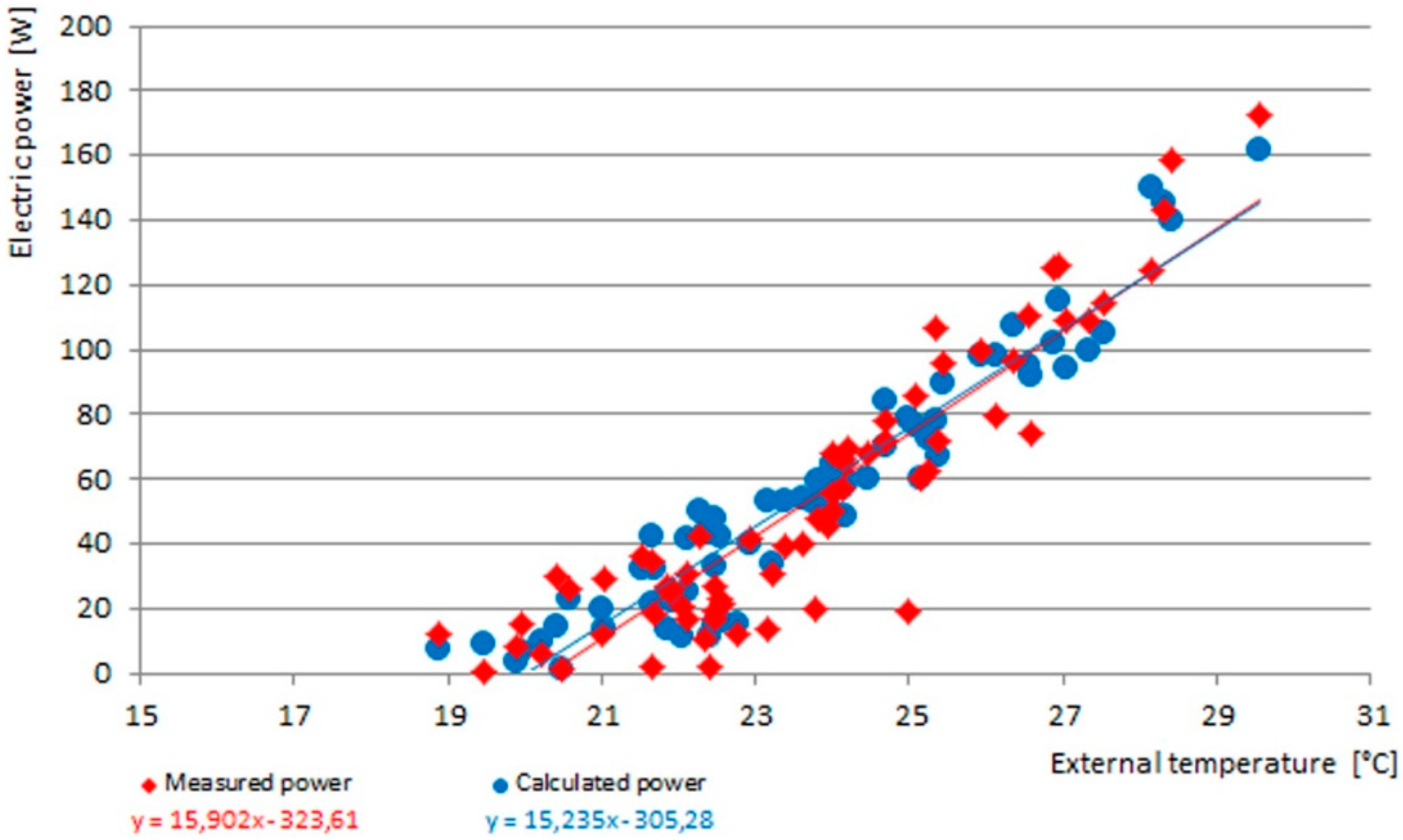
3.1. Model Results
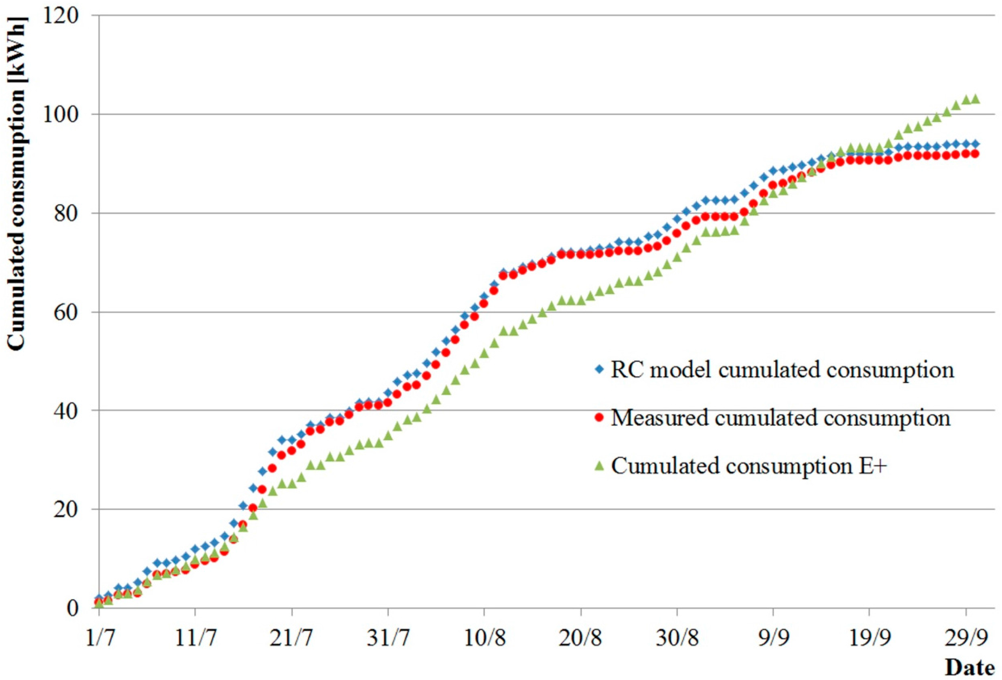
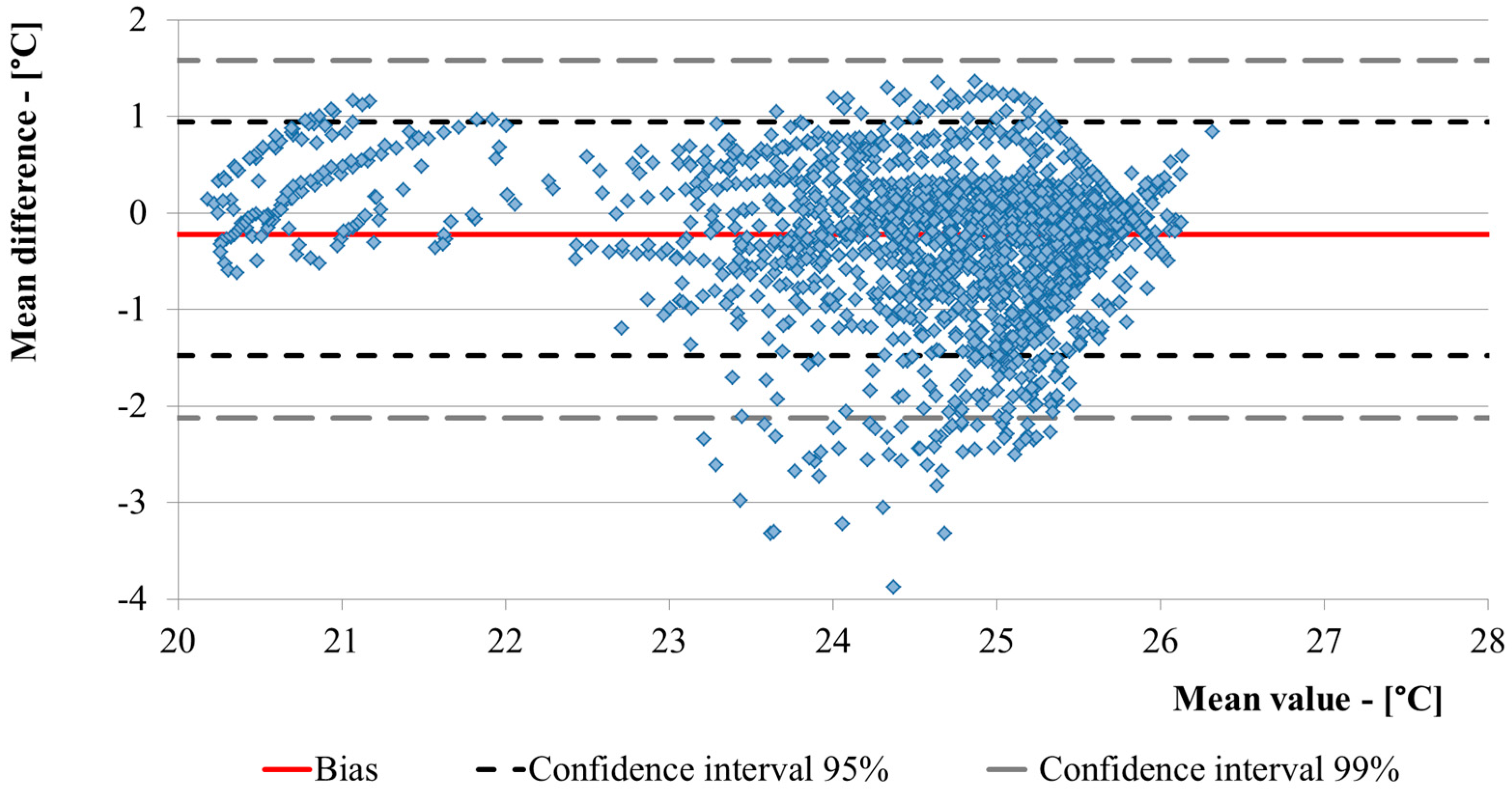
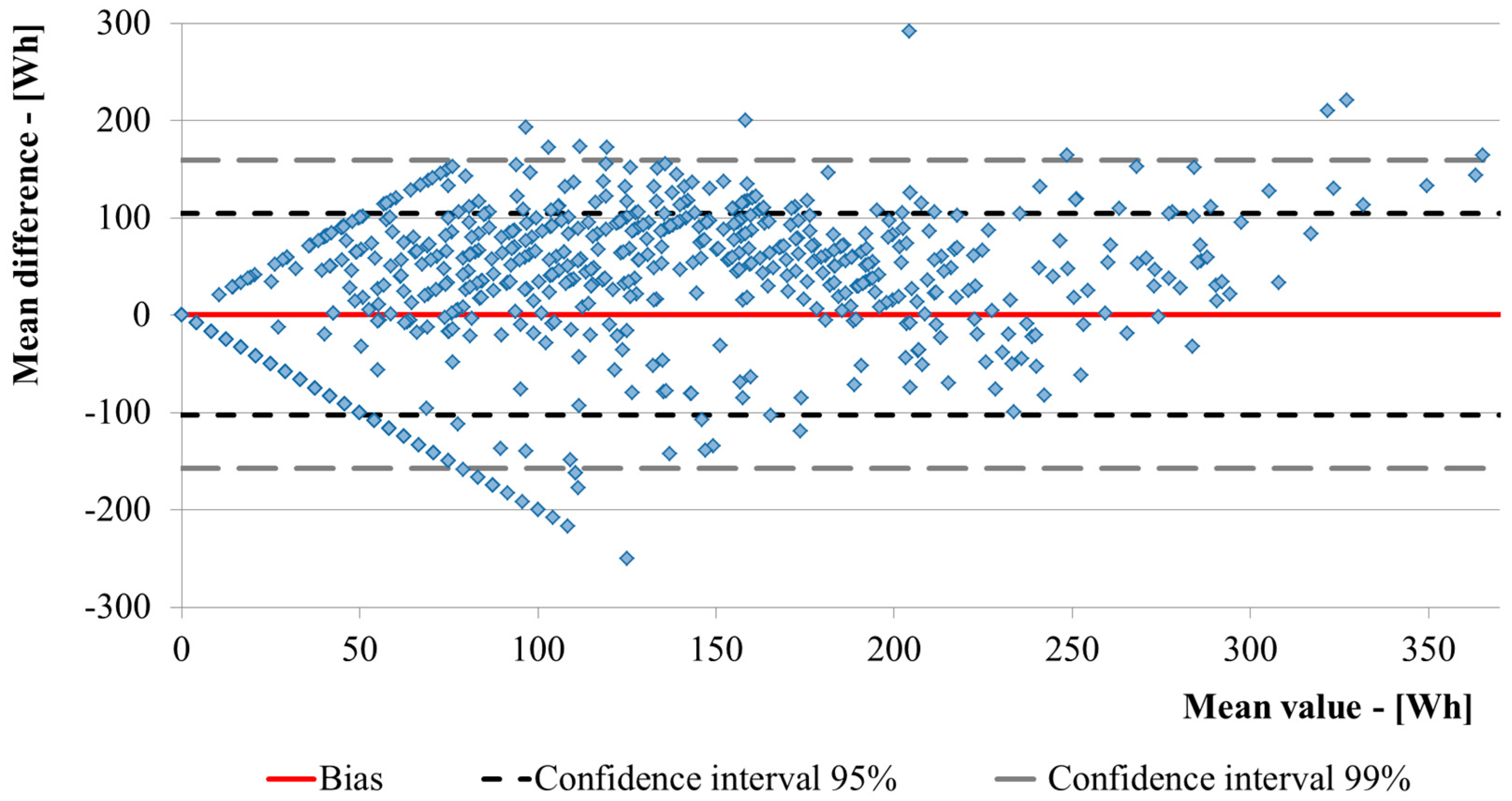
3.2. Validation
- is average differences,
- s is standard deviations.
4. Conclusions
Author Contributions
Conflicts of Interest
Nomenclature
| Symbol | Term | Unit |
| COP | Coefficient of Performance | – |
| EER | Energy Efficiency Ratio | – |
| Q | Heat load | MJ |
| W | Energy supplied | MJ |
| T | Temperature | K |
| η | Efficiency | – |
| ηII | Second law efficiency | – |
| Δp | Pressure difference | Pa |
| Δh | Enthalpy difference | kJ·kg−1 |
| DB | Dry Bulb | – |
| H | Heat transfer coefficient | W/K |
| C | Heat capacity | kJ/m2 |
| Φ | Heat flux | W/m2 |
Subscripts
| Symbol | Term |
| id | ideal |
| max | maximum |
| v | volumetric |
| iso | isentropic |
| h | hot source |
| c | cold source |
| h,1 | hot source supplied by the manufacturer |
| h,2 | hot source supplied by the manufacturer |
| c,1 | cold source supplied by the manufacturer |
| c2 | cold source supplied by the manufacturer |
| i | internal |
| e | external |
| s | surface |
| o | overall |
| tr | transmission |
References
- Directive 2012/27/EU of the European Parliament and of the Council of 25 October 2012 on Energy Efficiency, Amending Directives 2009/125/EC and 2010/30/EU and Repealing Directives 2004/8/EC and 2006/32/EC; The European Parliament and of the Council: Brussels, Belgium, 2012.
- Directive 2010/31/EU of the European Parliament and of the Council of 19 May 2010 on the Energy Performance of Buildings; The European Parliament and of the Council: Brussels, Belgium, 2010.
- Harish, V.S.K.V.; Kumar, A. A review on modeling and simulation of building energy systems. Renew. Sustain. Energy Rev. 2016, 56, 1272–1292. [Google Scholar] [CrossRef]
- Ji, Y.; Xu, P. A bottom-up and procedural calibration method for building energy simulation models based on hourly electricity submetering data. Energy 2015, 93, 2337–2350. [Google Scholar] [CrossRef]
- Terkaj, W.; Danza, L.; Devitofrancesco, A.; Gagliardo, S.; Ghellere, M.; Giannini, F.; Montic, M.; Pedriellia, G.; Sacco, M.; Salamone, F. A semantic framework for sustainable factories. Procedia CIRP 2014, 17, 547–552. [Google Scholar] [CrossRef]
- Gagliardo, S.; Giannini, F.; Monti, M.; Pedrielli, G.; Terkaj, W.; Sacco, M.; Ghellere, M.; Salamone, F. An ontology-based framework for sustainable factories. Comput. Aided Des. Appl. 2015, 12, 198–207. [Google Scholar] [CrossRef]
- Yan, D.; O’Brien, W.; Hong, T.; Feng, X.; Gunay, H.B.; Tahmasebi, F.; Mahdavi, A. Occupant behavior modeling for building performance simulation: Current state and future challenges. Energy Build. 2015, 107, 264–278. [Google Scholar] [CrossRef]
- Salamone, F.; Belussi, L.; Danza, L.; Ghellere, M.; Meroni, I. An open source low-cost wireless control system for a forced circulation solar plant. Sensors 2015, 15, 27990–28004. [Google Scholar] [CrossRef] [PubMed]
- Salamone, F.; Belussi, L.; Danza, L.; Ghellere, M.; Meroni, I. Design and development of nEMoS, an all-in-one, low-cost, web-connected and 3D-printed device for environmental analysis. Sensors 2015, 15, 13012–13027. [Google Scholar] [CrossRef] [PubMed]
- Salamone, F.; Belussi, L.; Danza, L.; Ghellere, M.; Meroni, I. An open source “smart lamp” for the optimization of plant systems and thermal comfort of offices. Sensors 2016, 16. [Google Scholar] [CrossRef] [PubMed]
- Zhu, M.; Pan, Y.; Huang, Z.; Xu, P. An alternative method to predict future weather data for building energy demand simulation under global climate change. Energy Build. 2016, 113, 74–86. [Google Scholar] [CrossRef]
- EN 15603:2008 Energy Performance of Buildings—Overall Energy Use and Definition of Energy Ratings; CEN-European Committee for Standardization: Brussels, Belgium, 2008.
- Van der Veken, J.; Saelens, D.; Verbeeck, G.; Hens, H. Comparison of steady-state and dynamic building energy simulation programs. In Proceedings of the International Buildings IX ASHRAE Conference on the Performance of Exterior Envelopes of Whole Buildings, Clearwater Beach, FL, USA, 5–10 December 2004.
- Doyle, M.D. Investigation of Dynamic and Steady State Calculation Methodologies for Determination of Building Energy Performance in the Context of the EPBD. Master’s Thesis, Dublin Institute of Technology, Dublin, Ireland, 2008. [Google Scholar]
- Gasparella, A.; Pernigotto, G. Comparison of quasi-steady state and dynamic simulation approaches for the calculation of building energy needs: Thermal losses. In Proceedings of the International High Performance Buildings Conference, West Lafayette, IN, USA, 16–19 July 2012.
- Belussi, L.; Danza, L.; Meroni, I.; Salamone, F.; Ragazzi, F.; Mililli, M. Energy performance of buildings: A study of the differences between assessment methods. In Energy Consumption: Impacts of Human Activity, Current and Future Challenges, Environmental and Socio-Economic Effects; Nova Science Publishers: New York, NY, USA.
- Wauman, B.; Breesch, H.; Saelens, D. Evaluation of the accuracy of the implementation of dynamic effects in the quasi steady-state calculation method for school buildings. Energy Build. 2013, 65, 173–184. [Google Scholar] [CrossRef]
- Fraisse, G.; Viardot, C.; Lafabrie, O.; Achard, G. Development of a simplified and accurate building model based on electrical analogy. Energy Build. 2002, 34, 1017–1031. [Google Scholar] [CrossRef]
- Kampf, J.H.; Robinson, D. A simplified thermal model to support analysis of urban resource flows. Energy Build. 2007, 39, 445–453. [Google Scholar] [CrossRef]
- Nielsen, T.R. Simple tool to evaluate energy demand and indoor environment in the early stages of building design. Sol. Energy 2005, 78, 73–83. [Google Scholar] [CrossRef]
- Ramallo-González, A.P.; Eames, M.E.; Coley, D.A. Lumped parameter models for building thermal modelling: An analytic approach to simplifying complex multi-layered constructions. Energy Build. 2013, 60, 174–184. [Google Scholar] [CrossRef] [Green Version]
- Park, H. Dynamic thermal modeling of electrical appliances for energy management of low energy buildings. In Electric Power; Universitè de Cergy Pontoise: Cergy Pontoise, France, 2013. [Google Scholar]
- Amara, F.; Agbossou, K.; Cardenas, A.; Dubé, Y.; Kelouwani, S. Comparison and simulation of building thermal models for effective energy management. Smart Grid Renew. Energy 2015, 6, 95–112. [Google Scholar] [CrossRef]
- Afram, A.; Janabi-Sharifi, F. Review of modeling methods for HVAC systems. Appl. Therm. Eng. 2014, 67, 507–519. [Google Scholar] [CrossRef]
- Fong, J.; Edge, J.; Underwood, C.; Tindale, A.; Potter, S. Performance of a dynamic distributed element heat emitter model embedded into a third order lumped parameter building model. Appl. Therm. Eng. 2015, 80, 279–287. [Google Scholar] [CrossRef]
- Cheung, H.; Braun, J.E. Component-based, gray-box modeling of ductless multi-split heat pump systems. Int. J. Refrig. 2014, 38, 30–45. [Google Scholar] [CrossRef]
- Costanzo, G.T.; Sossan, F.; Marinelli, M.; Bacher, P.; Madsen, H. Grey-box modeling for system identification of household refrigerators: A step toward smart appliances. In Proceedings of the IEEE 2013 4th International Youth Conference on Energy, 6–8 June 2013; pp. 1–5.
- Afram, A.; Janabi-Sharifi, F. Gray-box modeling and validation of residential HVAC system for control system design. Appl. Energy 2015, 137, 134–150. [Google Scholar] [CrossRef]
- Reay, D.A.; Macmichael, D.B.A. Heat Pumps; Elsevier: Oxford, UK, 1988. [Google Scholar]
- Crawley, D.B.; Pedersen, C.O.; Lawrie, L.K.; Winkelmann, F.C. EnergyPlus: Energy simulation program. ASHRAE J. 2000, 42, 49–56. [Google Scholar]
- Danza, L.; Barozzi, B.; Belussi, L.; Meroni, I.; Salamone, F. Assessment of the performance of a ventilated window coupled with a heat recovery unit through the co-heating test. Buildings 2016, 6, 3. [Google Scholar] [CrossRef]
- Nowak, T.; Jaganjacova, S.; Westring, P. European Heat Pump Market and Statistics Report; European Heat Pump Association: Brussels, Belgium, 2014. [Google Scholar]
- Hannon, M.J. Raising the temperature of the UK heat pump market: Learning lessons from Finland. Energy Policy 2015, 85, 369–375. [Google Scholar] [CrossRef]
- Cengel, Y.A. Introduction to Thermodynamics and Heat Transfer; McGraw-Hill Higher Education: Columbus, OH, USA, 2007. [Google Scholar]
- EN 15316-4-2:2008 Heating Systems in Buildings: Method for Calculation of System Energy Requirements and System Efficiencies; Part 4-2: Space Heating Generation Systems, Heat Pump Systems; CEN-European Committee for Standardization: Brussels, Belgium, 2008.
- Belussi, L.; Danza, L. Method for the prediction of malfunctions of buildings through real energy consumption analysis: Holistic and multidisciplinary approach of energy signature. Energy Build. 2012, 55, 715–720. [Google Scholar] [CrossRef]
- Belussi, L.; Danza, L.; Meroni, I.; Salamone, F. Energy performance assessment with empirical methods: Application of energy signature. Opto Electron. Rev. 2015, 23, 85–89. [Google Scholar] [CrossRef]
- Bland, J.M.; Altman, D.G. Statistical methods for assessing agreement between two methods of clinical measurement. Int. J. Nurs. Stud. 2010, 47, 931–936. [Google Scholar] [CrossRef]


| Efficiency Parameters | Nominal Condition | Value |
|---|---|---|
| Coefficient of Performance (COP) | 20 °C DB | 4.26 |
| 7 °C DB | ||
| Energy Efficiency Ratio (EER) | 27 °C DB | 4.00 |
| 35 °C DB |
| Indices | Average Differences between Calculated and Experimental Values— | Average Standard Deviations between Calculated and Experimental values—s | The 95% Confidence Interval | The 99% Confidence Interval |
|---|---|---|---|---|
| Indoor air temperature | −0.266 °C | 0.616 °C | 93.4 | 98.1 |
| Energy consumption | 0.989 Wh | 52.907 Wh | 92% | 98.7% |
© 2016 by the authors; licensee MDPI, Basel, Switzerland. This article is an open access article distributed under the terms and conditions of the Creative Commons by Attribution (CC-BY) license (http://creativecommons.org/licenses/by/4.0/).
Share and Cite
Danza, L.; Belussi, L.; Meroni, I.; Mililli, M.; Salamone, F. Hourly Calculation Method of Air Source Heat Pump Behavior. Buildings 2016, 6, 16. https://doi.org/10.3390/buildings6020016
Danza L, Belussi L, Meroni I, Mililli M, Salamone F. Hourly Calculation Method of Air Source Heat Pump Behavior. Buildings. 2016; 6(2):16. https://doi.org/10.3390/buildings6020016
Chicago/Turabian StyleDanza, Ludovico, Lorenzo Belussi, Italo Meroni, Michele Mililli, and Francesco Salamone. 2016. "Hourly Calculation Method of Air Source Heat Pump Behavior" Buildings 6, no. 2: 16. https://doi.org/10.3390/buildings6020016