An Isotropic Model for Cyclic Plasticity Calibrated on the Whole Shape of Hardening/Softening Evolution Curve


1
Politechnic Department of Engineering and Architecture (DPIA), University of Udine, via delle Scienze 208, 33100 Udine, Italy
2
Department of Engineering, University of Ferrara, via Saragat 1, 44122 Ferrara, Italy
*
Author to whom correspondence should be addressed.
Metals 2019, 9(9), 950; https://doi.org/10.3390/met9090950
Submission received: 14 June 2019
/
Revised: 14 August 2019
/
Accepted: 28 August 2019
/
Published: 30 August 2019
(This article belongs to the Special Issue Metal Plasticity and Fatigue at High Temperature)
Abstract
:This work presents a new isotropic model to describe the cyclic hardening/softening plasticity behavior of metals. The model requires three parameters to be evaluated experimentally. The physical behavior of each parameter is explained by sensitivity analysis. Compared to the Voce model, the proposed isotropic model has one more parameter, which may provide a better fit to the experimental data. For the new model, the incremental plasticity equation is also derived; this allows the model to be implemented in finite element codes, and in combination with kinematic models (Armstrong and Frederick, Chaboche), if the material cyclic hardening/softening evolution needs to be described numerically. As an example, the proposed model is applied to the case of a cyclically loaded copper alloy. An error analysis confirms a significant improvement with respect to the usual Voce formulation. Finally, a numerical algorithm is developed to implement the proposed isotropic model, currently not available in finite element codes, and to make a comparison with other cyclic plasticity models in the case of uniaxial stress and strain-controlled loading.
1. Introduction
Thanks to their favorable combination of mechanical and thermal properties, metals are widely employed in industrial applications in which components are subjected to high thermo-mechanical loadings. During the component’s service life, high temperatures combined with high mechanical stresses may induce in the component a plastic deformation, even only locally. If thermo-mechanical loadings also vary cyclically, the resulting cyclic elasto-plastic response may lead to some kind of fatigue damage. To perform a durability assessment, it is often advantageous to use a numerical approach based on the finite element (FE) method. The accuracy of results depends significantly on the capability of the material model, in the numerical code, to describe the cyclic plasticity behavior of the material, as it is observed experimentally.
A noteworthy example—considered in this work—is the case of copper alloys used in components of steel making plants (e.g., mold for continuous steel casting, anode for electric arc furnace, etc.) [1,2]. The material model in FE model needs to be calibrated on experimental cyclic plasticity data, which for copper alloys are rarely available in the literature. In [3], parameters for nonlinear kinematic and isotropic plasticity models were obtained for pure copper and CuCrZr alloys at a temperature range of between 20 °C and 550 °C. Cyclic hardening behavior of pure copper was studied in [4] but only limited to low-cycle fatigue curves. In a recent experimental study on CuAg0.1 [5], the identification of material parameters was performed with specific attention to nonlinear kinematic and isotropic models (Armstrong and Frederick, Chaboche and Voce), as generally they are already available in most common commercial finite element codes. While the kinematic model provided a quite precise fitting, the isotropic model (Voce) seemed less capable of following the softening trend of the CuAg0.1 alloy [5]. In fact, as it will be shown, the “S-shaped” curves characterizing the exponential law governing the Voce model hardly fitted the trend of experimental data, making the determination of the speed of stabilization fairly inaccurate. This aspect was already observed by [6,7] in the case of different types of steels. Neither the method—proposed in [8]—for changing the hardening modulus in the kinematic part, nor that proposed in [9] where the hardening model is obtained by superimposing several parts of kinematic and isotropic hardening, seem to solve the matter, as both appear only suitable for materials (like stainless steel) for which the hardening evolution depends on strain range. A possible way to capture more precisely a cyclic hardening/softening trend is that of superimposing two or more Voce models, as proposed in [10].
As the ability of plasticity models to accurately represent the material behavior plays an important role in numerical simulations and could have a direct influence on the accuracy of results, the aim of this work is to develop a new isotropic model that is able to replicate better the softening evolution of the copper alloy here investigated.
2. Materials and Methods
2.1. Experimental Testing
The experimental results of low-cycle fatigue (LCF) tests described in [5] are considered in this work. To characterize the cyclic stress-strain behavior and the fatigue strength of CuAg0.1 alloy (classified in ASTM B 124 standard [11]) at room and high temperature, strain-controlled tests with fully reversed (Rε = −1) triangular waveform at a strain rate of 0.01 s−1 were performed at three temperature levels (20 °C, 250 °C, 300 °C). However, only data at room temperature will be considered from now on.
2.2. Kinematic and Isotropic Plasticity Models: Theoretical Background
Plasticity is characterized by the irreversible straining that occurs once a certain level of stress is reached. If plastic strains are assumed to develop independently of time, several theories are available to characterize the response of materials. Plasticity theory distinguishes three main aspects: yield criterion, flow rule and material (hardening) models [12,13,14,15,16,17].
The yield criterion determines the stress level at which yielding occurs. In this work, the von Mises yield criterion is considered and the following expression of the plastic potential f is introduced [12,13,14]:
where is the deviatoric stress tensor, is the deviatoric part of the back stress, R is the drag stress and σ0 is the initial yield stress (bold symbols indicate tensors).
Once yielding occurs, a flow rule is needed to relate stresses and plastic strains. In the literature, several flow rules are available, nevertheless in the following the associated flow is adopted, in which the plastic flow is connected or associated with the yield criterion [12,13,14,15,16,17]:
The direction of the plastic strain increment dεpl depends on both the plastic multiplier dλ (non-negative scalar) and the plastic potential, which determine the amount and the direction of plastic straining, respectively.
Finally, hardening models (kinematic and isotropic) describe the change of yield surface as a function of plastic strain.
2.2.1. Kinematic Material Model
It is experimentally observed in metals under cyclic loading that the center of the yield surface moves in the direction of the plastic flow (the Bauschinger effect) [17]. A kinematic model captures the aforementioned effect, since it assumes that under a progressive yielding, the yield surface translates in the stress space, maintaining a constant size [12,15,16,17]. The translation of the yield surface center is described by the back stress X.
Different kinematic models have been developed to relate the increment of the back stress dX with the plastic strain εpl and usually also with the accumulated plastic strain dεpl,acc = (2/3dεpl:dεpl)1/2. For uniaxial loading dεpl,acc = dεpl [15].
The Prager model assumes that X is proportional to the plastic strain increment [12,13,14,15,16,17]:
where C is the hardening modulus. Armstrong and Frederick’s (AF) nonlinear model adds a recall term to Equation (3):
where γ is the non-linear recovery parameter that defines the rate at which the hardening modulus starts to decrease as the plastic strain develops. Finally, the Chaboche model is obtained by superimposing several AF models [8]:
2.2.2. Isotropic Material Model
The isotropic model assumes that, at any stage of loading, the center of the yield surface remains at the origin and the surface expands homotetically in size as plastic strain develops. Very often, a nonlinear isotropic model (known also as the Voce model [18]) is adopted. Expansion of the yield surface is described with the change of drag stress R [12,13,14,15]:
where b is the speed of stabilization and R∞ is the stabilized stress. Parameter R∞ can be positive or negative representing either cyclic hardening (R∞ > 0) or softening (R∞ < 0), respectively. Differentiation of Equation (6) gives [3,4,5,6,7,8,9,10,11,12,13,14,15]:
Furthermore, the evolution of R can also be interpreted as the relative change of the maximum stress σmax,i in the Nth cycle with respect to the maximum stress in the first (σmax,1) and in the stabilized (σmax,s) cycle [12,13,14]:
In case of strain-controlled loading, the plastic strain range per cycle ∆εpl is approximately constant and the plastic strain accumulated after N cycles becomes [12,14]:
Figure 1 plots Equation (8) for different values of b and versus the accumulated plastic strain on a log scale. As can be noticed, by increasing the speed of stabilization the curve shifts to the left, while its “S-shape” remains essentially unaffected. In other words, a material with a higher value of b reaches its stabilized condition at a lower value of εpl,acc (i.e., in a smaller number of cycles).
As with the kinematic model, also two or more Voce models can be superimposed, as proposed in [10]. Such a procedure requires a higher number of parameters to be estimated (minimum four: two parameters, b1 and b2, controlling the speed of stabilization and two others, R∞,1 and R∞,2, defining the stress saturation). While the sum R∞ = R∞,1 + R∞,2 clearly identifies the total saturated stress, the two components R∞,1 and R∞,2, taken individually, seem not to have a so evident physical meaning. The same observation holds true for parameter b in the original Voce model. If the model is described by more than one b, its physical meaning (i.e., speed of stabilization) seems to be lost, especially when one parameter is much bigger than the other (i.e., b1 >> b2). This observation is even more evident once the accelerated technique is adopted [19], in which the speed of stabilization is fictitiously increased. Generally, this approach is particularly suitable when dealing with computationally demanding simulations, i.e., in circumstances when small plastic strains occur during loading and a material model needs a huge number of cycles to reach a complete stabilization.
Finally, kinematic and isotropic models need to be jointly used if both the Bauschinger effect and the cyclic hardening/softening are to be simulated numerically.
2.2.3. Material Model Calibration
After having determined the static parameters (Young’s modulus and yield stress) as suggested in [12], kinematic variables were evaluated on experimental stabilized cycles at various strain amplitudes. This approach ensures that the estimated variables are suitable for being used over a wide range of strain amplitudes. Details on the estimation procedure (Young’s modulus, yield stress and kinematic variables) is given in [5,20,21].
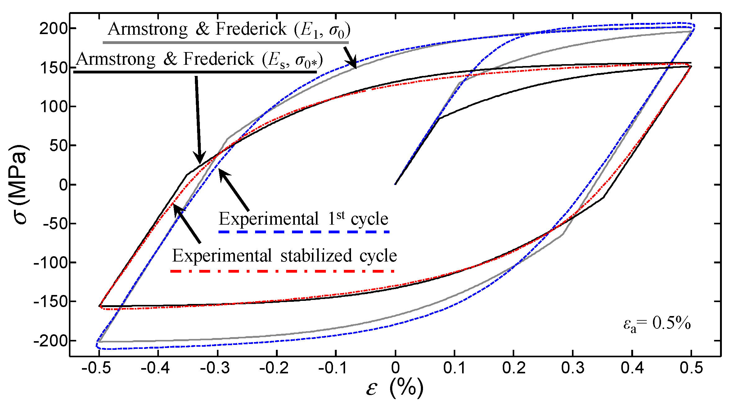
Figure 2 compares the simulated cycles (only kinematic model) with the first and stabilized experimental cycles, for εa = 0.5%. For the considered material, the Armstrong and Frederick kinematic model (parameters C, γ) is selected, as it yields a better agreement with experiments, than does the Chaboche model (see [5]). For the first simulated cycle, the initial values of Young’s modulus and the yield stress are assumed. As can be noticed, the model stabilizes in the first two cycles and agrees fairly well with the experimental cycle. In addition, Figure 2 also depicts the stabilized stress-strain cycle (black solid line) obtained with the stabilized parameters (Es, σ0*). The change from the first cycle to the stabilized one confirms a softening behavior for the material.
Nonlinear isotropic parameters were then estimated according to Voce model. The maximum stress σmax was measured for each stress-strain cycle. As the CuAg0.1 alloy never saturates completely, the stabilized stress σmax,s does not approach any asymptote and its value was then established by a conventional criterion, which considered the maximum stress at half the number of cycles to failure. The procedure was repeated for each strain amplitude. According to Equation (8), the saturation stress R∞ was determined as:
In this case, R∞ < 0, i.e., material exhibits softening (see also Figure 2). The speed of stabilization b was identified by fitting Equation (8) to experiments. Figure 3 compares the isotropic model curve and experiments for εa = 0.5%. A satisfactory correlation is obtained, particularly at the smallest and the largest values of accumulated plastic strain (i.e., at the first and saturated cycle, respectively). Other than that, the model follows a trend that deviates significantly from that followed by experimental data. A similar inconsistency was also observed for other strain amplitudes. The aim to improve the fitting accuracy then motivates the attempt to modify the evolution rule of R in a new isotropic model, described in the next paragraph.
3. Proposed Isotropic Model
As previously observed, experimental results obtained for CuAg0.1 alloy do not fit perfectly well with the “S-shape” curve of the exponential law proposed by Voce. With the aim to get an improved fitting with experiments, a new model described by the following equation is thus proposed:
in which a, s are material parameters that control the rate of cyclic hardening or softening. The proposed expression has a physical basis being it able to capture the two limiting cases: R = 0 for εpl,acc→0 and R = R∞ for εpl,acc→∞. Differentiation of Equation (11) gives the incremental relationship:
Similarly, to the Voce model, the evolution of R can be described by the relative change of maximum stress in each cycle:
Fitting of Equation (13) to experimental data yields the values of a and s parameters. The estimation procedure to evaluate the saturation stress R∞ remains unchanged.
Figure 4 displays a sensitivity analysis of Equation (13), which is helpful to clarify the physical meaning of parameters a and s. At increasing values of a (keeping s constant), the speed of stabilization diminishes and the curve shifts to the right. In other words, a bigger amount of accumulated plastic strain is needed to reach the stabilized condition, see Figure 4a. By contrast, the exponent s (keeping a constant) controls the “slope” of the increasing portion of the curve (i.e., higher values of s give a steeper average slope), see Figure 4b.
Please note that limiting values exist for both parameters. For example, no cyclic hardening/softening would actually occur if a becomes either infinite (for which R = 0 for any s) or zero (for which R = R∞ from the first cycle). A similar behavior also occurs when s = 0, for which R = R∞/(a + 1) (in the example of Figure 4, R ≅ 0.667R∞). When s increases to infinite, R = 0 for εpl,acc < 1, R = R∞ for εpl,acc > 1 and R = R∞/(a + 1) for εpl,acc = 1.
4. Results and Discussion
The nonlinear kinematic model is able to capture quite accurately the first and the stabilized cycle, if the initial and stabilized static parameters are adopted, respectively, see Figure 2. However, the combined (kinematic and isotropic) model is needed, if the cyclic softening evolution of CuAg0.1 alloy has to be considered. It is then of interest to discuss in more detail on the results obtained with both the Voce and the new isotropic model proposed in this work.
4.1. Stress-Strain Behavior: Isotropic Model (Voce)
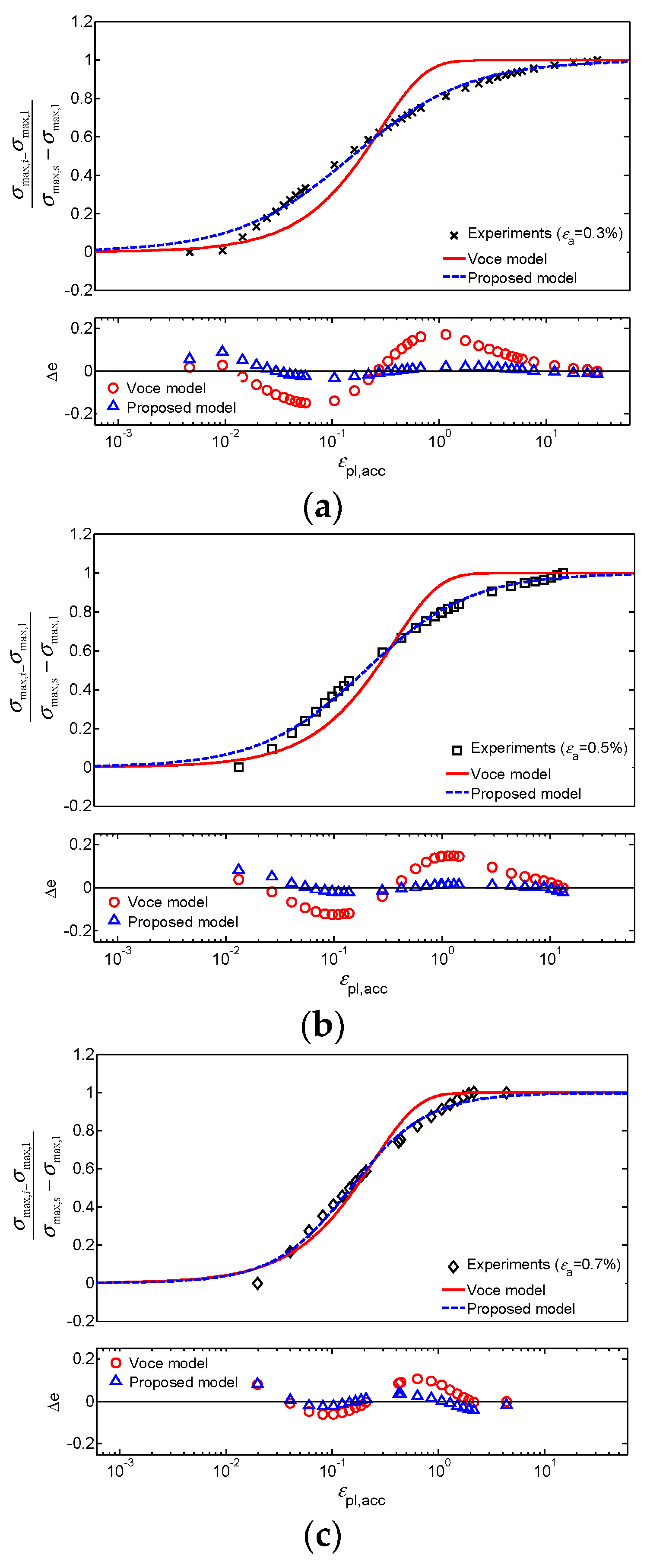
The solid lines in Figure 5 show how Equation (8) fits the cyclic data for εa = 0.3%, 0.5% and 0.7%. The corresponding three estimated values of b are reported in Table 1 (along with the values estimated for other strain amplitudes). As it can be noticed, in all three cases examined the fitting curve does not match experimental data perfectly. In fact, experiments follow a quite smoother trend with respect to the “S-shaped” curve given by the exponential expression in Equation (8). On the other hand, it was already observed and shown in Figure 1 that the speed of stabilization b only makes the S-curve shift horizontally, without changing its shape.
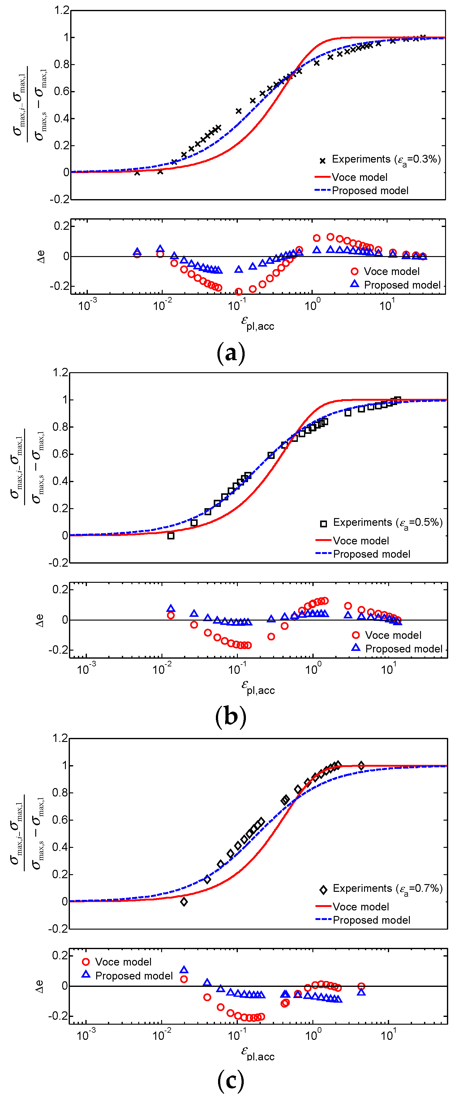
Different values of b and R∞ characterize cycles with different strain amplitude values, see Table 1. This may represent a drawback, if commercial finite element codes have to be used, as they generally permit only one single value of the isotropic parameters to be input. On the other hand, a component may be subjected to a certain loading condition, for which the resulting plastic strain spans over a relatively wide range. A possible compromise for solving this issue could be to take an average value R∞,ave and to identify a single value ball by fitting Equation (8) to all the experimental data gathered together (see the last row in Table 1), as it was done in Figure 11 in [5]. A comparison between the fitted curve calculated with ball and the experimental data is presented in Figure 6. As expected, this “averaging” procedure makes the fitting even worse with respect to the previous case.
4.2. Stress-Strain Behavior: Proposed Isotropic Model
Figure 5 also compares the proposed model (blue dashed line) with the same experimental data (εa = 0.3%, 0.5% and 0.7%) considered previously for the Voce model. It is apparent how Equation (13) yields a more precise fitting with experiments.
Also for this model, a range of values for a (0.101÷0.514) and s (0.802÷1.203) characterize cycles with different strain amplitudes, see Table 1. Therefore, similarly to the case of Voce model, single values of aall, sall were estimated by fitting Equation (13) to all the experimental data gathered together. Table 1 then lists the values of a, s for each strain amplitude, as well as the “averages” aall, sall (see the last row). A comparison is presented in Figure 6. Even now, as it was for the previous comparison, for all three amplitudes examined the new isotropic model is far closer to experiments than Voce model is.
For the proposed model is not yet possible to prescribe a range of a and s values of general validity, as it would be desirable to have additional data from other materials.
4.3. Error Analysis
The previous comparison—clearly more qualitative—can be made more quantitative by the use of suitable error metrics through which the deviation of each model from experimental data can be quantified and compared.
Residual (∆e) and sum of squares of residuals (SSE) are used to measure the deviation between model and experiments. The residual provides a “local” measure of fitting at each point, whereas the SSE index gives a “global” measure of fitting. The residual measures the difference for each experimental point used in model calibration and it is defined as [22]:
where:
Symbol n denotes the number of experimental points used in calibration.
The bottom graph in Figure 5 and Figure 6 show the values of residuals for both isotropic models, at three different strain amplitudes (εa = 0.3%, 0.5%, 0.7%). Figure 5 refers to specific values (b, a, s) for the three amplitudes; Figure 6 refers to the “average” parameters (ball, aall, sall), calculated as explained before. The residuals ∆e are plotted on the vertical axis while the accumulated plastic strain, which is an independent variable, is plotted on the horizontal axis. In all considered cases, residual ∆e obtained with the proposed model is significantly smaller with respect to Voce model. The maximum percentage residual for the considered strain amplitudes varies over a range of 44–51% and 5–18%, respectively, for the Voce and the proposed models.
To provide a single index value that quantifies the model accuracy for each strain amplitude, the sum of squares of residuals is also calculated [22]:
Values of SSE, calculated for each strain amplitude, are listed in Table 1. Both models give the biggest SSE for εa = 0.15% and εa = 0.175%. These large values can be explained by considering that at those small strain amplitudes, the CuAg0.1 alloy showed a slight hardening in the first 5–10 cycles, after which softening occurred, as observed in [5]. Such a small hardening at the beginning of loading gives an increment of the maximum stress σmax,i with respect to the initial value σmax,1. A positive difference σmax,i–σmax,1 results and thus a negative ratio in the left-hand side of Equations(8) and (13) appears. As Equations (8) and (13) are always positive and bounded by two horizontal asymptotes at both tails, such an initial hardening cannot be captured correctly and inevitably a small error is introduced in the fitting. At other strain amplitudes (0.2–07%), the proposed model gives from 75% up to 94% lower values of SSE with respect to the Voce model, see Table 1.
As expected, see Table 2, the fitting curves obtained by the parameters (ball, aall, sall) are slightly less accurate than those obtained by the parameters (b, a, s) in Table 1 that were specifically calibrated for each strain amplitude. Nevertheless, it can be noticed that the proposed model always provides considerably better results in terms of SSE with respect to Voce model.
4.4. Combined Armstrong-Frederick with Proposed Isotropic Model: Stress-Strain Evolution
A numerical algorithm is developed, see Appendix A, to implement the combined kinematic and proposed isotropic plasticity model, in the case of uniaxial stress and strain-controlled loading.
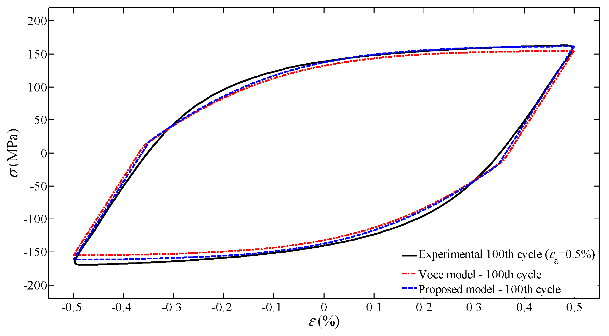
Figure 7 displays the stress-strain evolution at the 100th cycle for strain amplitude εa = 0.5%. Although the difference between the three curves is relatively small, the proposed model fits more precisely the experimental stress-strain curve.
As a final remark, the cyclic hardening/softening evolution described with Equations (6) and (11) only depends on the accumulated plastic strain, but not on the plastic strain amplitude. This implies that all experimental data should collapse into one single curve independently on the imposed strain amplitude. On the other hand, the literature reports examples of materials—e.g., 316 stainless steel [12,13,14], nickel base superalloy [23] and 42CrMo4 steel [7]—for which the isotropic behavior depends on the strain amplitude. For the CuAg0.1 alloy considered in this work, such a dependence is not so evident, but cannot be excluded at all. Therefore, a further analysis in that sense would be desirable.
5. Conclusions
In this work, a new isotropic model is proposed for describing the cyclic hardening/softening behavior of metals. The model is an attempt to overcome the poor fitting observed in Voce isotropic model, when calibrated on experimental cyclic data of a CuAg0.1 alloy. Strain-controlled cyclic test data at different strain amplitudes, carried out in a recent study published by the authors, are used as a benchmark. Experimental data were used for identifying parameters of non-linear kinematic (Armstrong and Frederick, Chaboche) and isotropic (Voce) models. The calibration identified the one-pair kinematic model as the closest to experiments. By contrast, a poor agreement was observed when fitting the isotropic Voce model. The discrepancy is attributed to the fact that experiments follow a smoother trend with respect to the “S-shaped” curve defined by the exponential expression of Voce model equation. In fact, the Voce model is described by two parameters, i.e., the stabilized stress R∞ and the speed of stabilization b, the latter only shifting the curve horizontally, while keeping the curve shape unaffected.
An improved isotropic model, aimed at providing a better fit with experimental data, is then proposed and calibrated to the same experimental data. In addition to the stabilized stress R∞ also present in Voce model, the proposed model is governed by two parameters a, s, which both control the speed of stabilization and the shape of the hardening/softening evolution curve. An error analysis on calibration results confirms that the proposed model is much closer to experiments than Voce model in all cases examined.
The proposed isotropic model, when combined with the kinematic one, seems to better fit the experimental stress-strain curves than the Voce model combined with the same kinematic part. This permits the cyclic hardening/softening evolution of the material to be described quite accurately.
Finally, a numerical algorithm is developed to implement the combined kinematic and proposed isotropic plasticity model, in the case of uniaxial stress and strain-controlled loading. The framework of the presented algorithm permits convergence to be always achieved with low computational cost.
Author Contributions
Conceptualization: J.S.N. and D.B.; methodology: J.S.N., F.D.B. and D.B.; software: J.S.N.; validation: J.S.N., F.D.B. and D.B.; investigation: J.S.N., F.D.B. and, D.B., writing-original draft preparation: J.S.N., F.D.B. and D.B.; writing-review and editing: J.S.N., F.D.B. and D.B.; supervision: F.D.B. and D.B.
Funding
This research received no external funding.
Conflicts of Interest
The authors declare no conflict of interest. The research was conducted without personal financial benefit from any funding body, and no such body influenced the execution of the work.
Appendix A
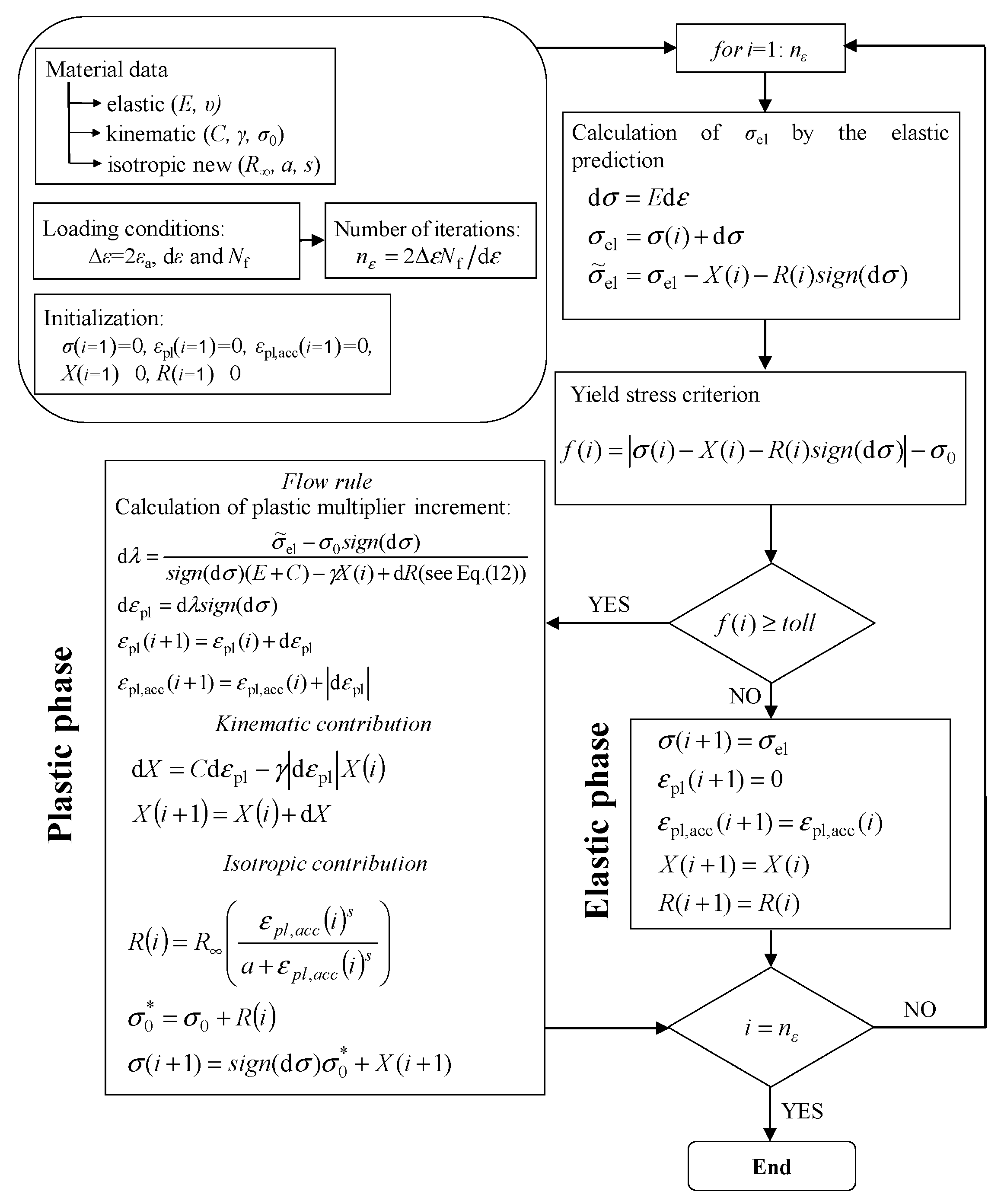
A numerical algorithm is developed to implement the proposed model, currently not available in numerical codes. The algorithm applies to the case of uniaxial stress and strain-controlled loading (constant strain range) and it permits a comparison between the combined models (kinematic-Voce and kinematic-proposed model) and experimental data.
Figure A1 sketches the block diagram of the numerical algorithm. The calculation starts by defining the strain range Δε = 2εa, the strain increment dε and the number of cycles Nf to be simulated. The number of iterations nε is obtained dividing 2ΔεNf by dε.
The stress increment is computed based on the strain increment assuming that the stress-strain relation is completely elastic. The elastic stress predictor σel is then evaluated simply adding to σi the stress increment dσ. In the same iteration, the actual yield stress remains unchanged and the plastic strain is set to be zero. If the elastic stress predictor indicates that yield stress has been exceeded (von Mises yield criterion is adopted), the increment becomes elasto-plastic. Consequently, the plastic strain increment dεpl has to be calculated by adopting a flow rule. For von Mises criterion, the plastic multiplier dλ corresponds to the increment of plastic strain; for uniaxial loading the accumulated plastic strain increment dεpl,acc is equal to dεpl [15] and therefore the accumulated plastic strain can be evaluated accordingly. Finally, the (i + 1)th value of stress is determined by taking into account the contribution of the back stress X and of the drag stress R (kinematic and isotropic) with Equations (4) and (11), respectively.
Figure A1.
Calculation of stress-strain evolution considering uniaxial case with combined nonlinear kinematic and proposed isotopic models.
Figure A1.
Calculation of stress-strain evolution considering uniaxial case with combined nonlinear kinematic and proposed isotopic models.
References
- Moro, L.; Benasciutti, D.; De Bona, F. Simplified numerical approach for the thermo-mechanical analysis of steelmaking components under cyclic loading: An anode for electric arc furnace. Ironmaking Steelmaking 2019, 46, 56–65. [Google Scholar] [CrossRef]
- Moro, L.; Srnec Novak, J.; Benasciutti, D.; De Bona, F. Thermal distortion in copper moulds for continuous casting of steel: Numerical study on creep and plasticity effect. Ironmaking Steelmaking 2019, 46, 97–103. [Google Scholar] [CrossRef]
- You, J.H.; Miskiewicz, M. Material parameters of copper and CuCrZr alloy for cyclic plasticity at elevated temperatures. J. Nucl. Mater 2008, 373, 269–274. [Google Scholar] [CrossRef] [Green Version]
- Hatanaka, K.; Yamada, T.; Hirose, Y. An effective plastic strain component for low cycle fatigue in metals. JSME 1980, 23, 791–797. [Google Scholar] [CrossRef]
- Benasciutti, D.; Srnec Novak, J.; Moro, L.; De Bona, F.; Stanojevic, A. Experimental characterization of a CuAg alloy for thermo-mechanical applications. Part 1: Identifying parameters of non-linear plasticity models. Fatigue Fract. Eng. Mater Struct. 2018, 41, 1364–1377. [Google Scholar] [CrossRef]
- Goodall, I.W.; Hales, R.; Walters, D.J. On constitutive relations and failure criteria of an austenitic steel under cyclic loading at elevated temperature. In IUTAM Symp. Creep in Structures; Ponter, A.R.S., Hayhurst, D.R., Eds.; Springer: Leicester, UK, 1980; pp. 103–127. [Google Scholar]
- Basan, R.; Franulovic, M.; Prebil, I.; Kunc, R. Study on Ramberg-Osgood and Chaboche models for 42CrMo4 steel and some approximations. J. Constr. Steel Res. 2017, 136, 65–74. [Google Scholar] [CrossRef]
- Chaboche, J.L. Constitutive equations for cyclic plasticity and cyclic viscoplasticity. Int. J. Plast. 1989, 5, 247–302. [Google Scholar] [CrossRef]
- Kang, G.; Ohno, N.; Nebu, A. Constitutive modeling of strain range dependent cyclic hardening. Int. J. Plast. 2003, 19, 1801–1819. [Google Scholar] [CrossRef]
- Chaboche, J.L.; Dang Van, K.; Cordier, G. Modelization of the strain memory effect on cyclic hardening of 316 stainless steel. In Proceedings of the Conference on Structural Mechanics in Reactor Technology, SMiRT 5, Berlin, Germany; 1979. [Google Scholar]
- ASTM B 124-B 124M. Standard Specification for Copper and Copper Alloy Forging Rod, Bar, and Shapes; ASTM International: West Conshohocken, PA, USA, 2008. [Google Scholar]
- Lemaitre, J.; Chaboche, J.L. Mechanics of Solid Materials; Cambridge University Press: Cambridge, UK, 1990. [Google Scholar]
- Chaboche, J.L. A review of some plasticity and viscoplasticity constitutive theories. Int. J. Plast. 2008, 24, 1642–1693. [Google Scholar] [CrossRef]
- Chaboche, J.L. Time-independent constitutive theories for cyclic plasticity. Int. J. Plast. 1986, 2, 149–188. [Google Scholar] [CrossRef]
- Dunne, F.; Petrinic, N. Introduction to Computational Plasticity; Oxford University Press: New York, NY, USA, 2005. [Google Scholar]
- Chen, W.F.; Zhang, H. Plasticity for Structural Engineers; Springer: New York, NY, USA, 1988. [Google Scholar]
- Simo, J.C.; Hughes, T.J.R. Computational Inelasticity; Springer: New York, NY, USA, 1998. [Google Scholar]
- Voce, E. A practical strain hardening function. Metallurgia 1955, 51, 219–226. [Google Scholar]
- Chaboche, J.L.; Cailletaud, G. On the calculation of structures in cyclic plasticity or viscoplasticity. Comput. Struct. 1986, 23, 23–31. [Google Scholar] [CrossRef]
- Novak, S.J.; Stanojevic, A.; Benasciutti, D.; De Bona, F.; Huter, P. Thermo-mechanical finite element simulation and fatigue life assessment of a copper mould for continuous casting of steel. Procedia Eng. 2015, 133, 688–697. [Google Scholar] [CrossRef]
- Novak, S.J.; Benasciutti, D.; De Bona, F.; Stanojevic, A.; De Luca, A.; Raffaglio, Y. Estimation of material parameters in nonlinear hardening plasticity models and strain life curves for CuAg alloy. Mater. Sci. Eng. 2016, 119, 1–9. [Google Scholar] [CrossRef]
- Montgomery, D.C.; Runger, G.C. Applied Statistics and Probability for Engineers, 6th ed.; John Wiley Sons: Hoboken, NJ, USA, 2014. [Google Scholar]
- Zhao, L.G.; Tong, B.; Vermeulen, B.; Byrne, J. On the uniaxial mechanical behaviour of an advanced nickel base superalloy at high temperature. Mech. Mater. 2001, 33, 593–600. [Google Scholar] [CrossRef]
Figure 1.
Plot of Equation (8) for different values of b parameter.
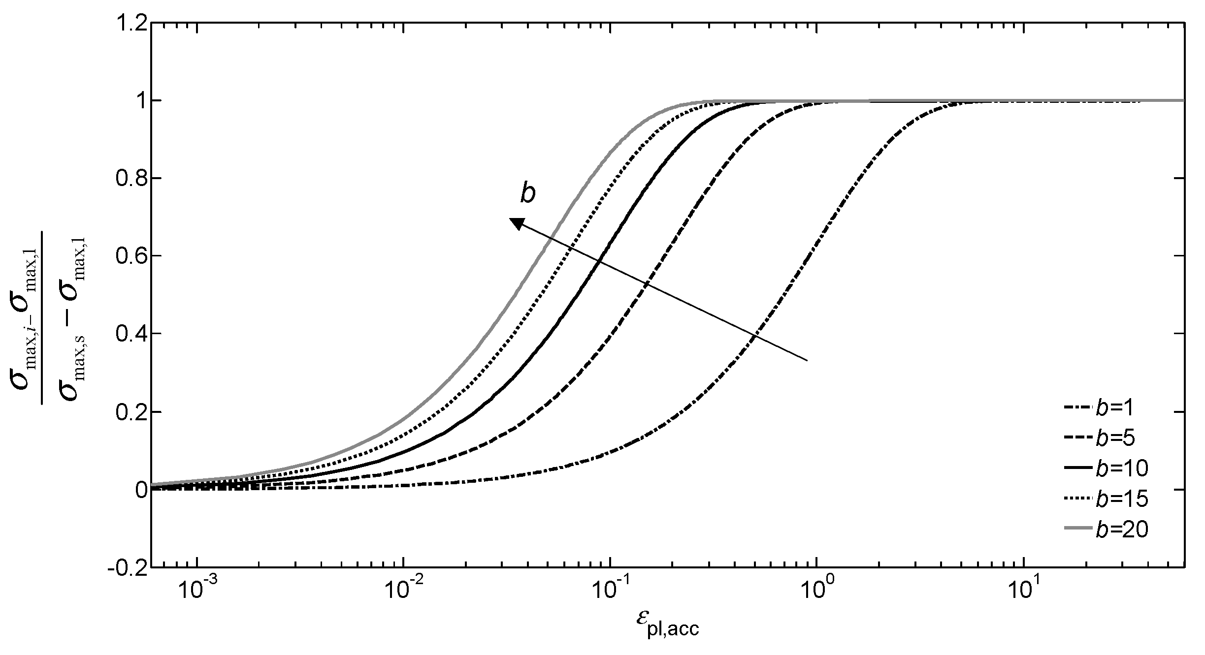
Figure 2.
Comparison between simulated and experimental (first and stabilized) cycle.

Figure 3.
Experimental data for εa = 0.5% (markers) fitted by the isotropic model.
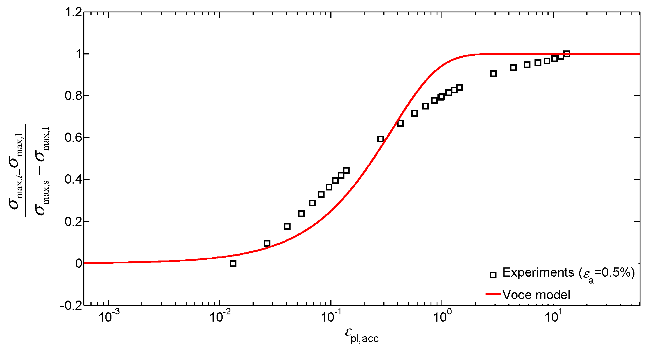
Figure 4.
The sensitivity of the proposed Equation (10) to parameters (a) a and (b) s.

Figure 5.
Isotropic model for different strain amplitudes ((a) εa = 0.3%, (b) εa = 0.5% and (c) εa = 0.7%); Voce model (red solid line) and proposed model (blue dashed line). Residual ∆e is also reported.
Figure 5.
Isotropic model for different strain amplitudes ((a) εa = 0.3%, (b) εa = 0.5% and (c) εa = 0.7%); Voce model (red solid line) and proposed model (blue dashed line). Residual ∆e is also reported.

Figure 6.
Isotropic model for different strain amplitudes ((a) εa = 0.3%, (b) εa = 0.5% and (c) εa = 0.7%) calculated with ball, aall and sall parameters; Voce model (red solid line) and proposed model (blue dashed line). Residual ∆e is also reported.
Figure 6.
Isotropic model for different strain amplitudes ((a) εa = 0.3%, (b) εa = 0.5% and (c) εa = 0.7%) calculated with ball, aall and sall parameters; Voce model (red solid line) and proposed model (blue dashed line). Residual ∆e is also reported.

Figure 7.
Stress-strain evolution of 100th cycle for strain amplitude εa = 0.5%, comparison between experiments, combined model with Voce and with proposed isotropic models.
Figure 7.
Stress-strain evolution of 100th cycle for strain amplitude εa = 0.5%, comparison between experiments, combined model with Voce and with proposed isotropic models.

Table 1.
Isotropic parameters identified from experimental data for the Voce and proposed models. Goodness-of-fit examined in terms of sum of squares of residuals (SSE) for each model and strain amplitude.
Table 1.
Isotropic parameters identified from experimental data for the Voce and proposed models. Goodness-of-fit examined in terms of sum of squares of residuals (SSE) for each model and strain amplitude.
| Strain Amplitude | Material Parameters | Error Index (SSE) | ||||
|---|---|---|---|---|---|---|
| εa | R∞ (MPa) | Voce | Proposed | Voce | Proposed | |
| b | a | s | ||||
| 0.15% | −56 | 1.307 | 0.514 | 0.923 | 1.914 | 1.601 |
| 0.175% | −71 | 1.197 | 0.491 | 0.978 | 0.654 | 0.455 |
| 0.2% | −80 | 3.145 | 0.316 | 0.778 | 0.464 | 0.063 |
| 0.3% | −84 | 3.620 | 0.223 | 0.802 | 0.338 | 0.022 |
| 0.4% | −83 | 4.488 | 0.179 | 0.855 | 0.292 | 0.016 |
| 0.5% | −52 | 2.871 | 0.234 | 0.893 | 0.269 | 0.014 |
| 0.6% | −52 | 2.581 | 0.290 | 0.853 | 0.298 | 0.019 |
| 0.7% | −69 | 4.208 | 0.101 | 1.203 | 0.069 | 0.017 |
| Single values | R∞,ave1 | ball1 | aall1 | sall1 | 3.401 | 1.766 |
| −68 | 2.352 | 0.199 | 0.965 | |||
1 parameters ball, aall and sall are estimated from all experimental data merged together (whereas R∞,ave is the average over all strain values).
Table 2.
Evaluation of fitted curves obtained with both models and calculated with ball, aall and sall.
Table 2.
Evaluation of fitted curves obtained with both models and calculated with ball, aall and sall.
| Strain Amplitude | Error Index (SSE) | |
|---|---|---|
| εa | Voce | Proposed |
| 0.3% | 0.493 | 0.080 |
| 0.5% | 0.289 | 0.021 |
| 0.7% | 0.340 | 0.094 |
© 2019 by the authors. Licensee MDPI, Basel, Switzerland. This article is an open access article distributed under the terms and conditions of the Creative Commons Attribution (CC BY) license (http://creativecommons.org/licenses/by/4.0/).
Share and Cite
MDPI and ACS Style
Srnec Novak, J.; De Bona, F.; Benasciutti, D. An Isotropic Model for Cyclic Plasticity Calibrated on the Whole Shape of Hardening/Softening Evolution Curve. Metals 2019, 9, 950. https://doi.org/10.3390/met9090950
AMA Style
Srnec Novak J, De Bona F, Benasciutti D. An Isotropic Model for Cyclic Plasticity Calibrated on the Whole Shape of Hardening/Softening Evolution Curve. Metals. 2019; 9(9):950. https://doi.org/10.3390/met9090950
Chicago/Turabian StyleSrnec Novak, Jelena, Francesco De Bona, and Denis Benasciutti. 2019. "An Isotropic Model for Cyclic Plasticity Calibrated on the Whole Shape of Hardening/Softening Evolution Curve" Metals 9, no. 9: 950. https://doi.org/10.3390/met9090950
Note that from the first issue of 2016, this journal uses article numbers instead of page numbers. See further details here.