Finite Element Analysis on a Newly-Modified Method for the Taylor Impact Test to Measure the Stress-Strain Curve by the Only Single Test Using Pure Aluminum


1
Graduate School of Engineering, Hiroshima University, 1-4-1 Kagamiyama, Higashi-Hiroshima 739-8527, Japan
2
Academy of Science and Technology, Hiroshima University, 1-4-1 Kagamiyama, Higashi-Hiroshima 739-8527, Japan
*
Author to whom correspondence should be addressed.
Metals 2018, 8(8), 642; https://doi.org/10.3390/met8080642
Submission received: 20 July 2018
/
Revised: 6 August 2018
/
Accepted: 13 August 2018
/
Published: 15 August 2018
(This article belongs to the Special Issue Deformation Behavior of the Alloys under Simple and Combined Loading Conditions at Various Deformation Rate)
Abstract
:In this study, finite element analyses are performed to obtain a stress-strain curve for ductile materials by a combination between the distributions of axial stress and strain at a certain time as a result of one single Taylor impact test. In the modified Taylor impact test proposed here, a measurement of the external impact force by the Hopkinson pressure bar placed instead of the rigid wall, and an assumption of bi-linear distribution of an axial internal force, are introduced as well as a measurement of deformed profiles at certain time. In order to obtain the realistic results by computations, at first, the parameters in a nonlinear rate sensitive hardening law are identified from the quasi-static and impact tests of pure aluminum at various strain rates and temperature conducted. In the impact test, a miniaturized testing apparatus based on the split Hopkinson pressure bar (SHPB) technique is introduced to achieve a similar level of strain rate as 104 s−1, to the Taylor test. Then, a finite element simulation of the modified test is performed using a commercial software by using the user-subroutine for the hardening law with the identified parameters. By comparing the stress-strain curves obtained by the proposed method and direct calculation of the hardening law, the validity is discussed. Finally, the feasibility of the proposed method is studied.
1. Introduction
The Taylor impact test, established by Taylor [1], is a quite simple impact compressive test. In this test, a cylindrical slender specimen is shot to, and strikes the surface of a rigid body wall. After striking, the length of the deformed specimen is measured to determine the mechanical properties of the materials. As a result of the test, maximum strain rates as high as 103–105 s−1 can be easily obtained. The test is applicable to a wide variety of materials such as metals [2], polymers [3,4], foams [5,6] etc. The test was originally used for measuring the impact yield strength, and the fairly reliable value of the strength can be obtained.
It is actively discussed that modifications to the theoretical formulae in the original method are needed to calculate the strength, because only constant deceleration at the free end of specimens is considered. For example, Wilkins and Guinan [7] experimentally derive the conclusion that the ratio between length in the region due to plastic deformation and the total length of the deformed specimen is almost constant, with respect to the impact velocity, and they propose a simplification method of the formulae by Taylor [1]. In order to reduce the effect of friction and to avoid the indentation of the wall by specimens, the symmetric Taylor impact test [8,9] is also proposed.
In conjunction with the above discussions in terms of the Taylor impact test, a further modification is made to measure a stress-strain curve of ductile materials. Jones et al. [10,11] extend the theoretical formulae by including not only the yield stress, but also work hardening effect. Julien et al. [12] made a big challenge to measure stress-strain curve in brass, based on the test, by using various kinds of formulae, as well as formulae by Jones et al. [10,11] to compare between them. However, according to their method, numerous repetitions of the experiments are necessary to obtain one single stress-strain curve. In addition, these formulae only considering the deformation of the specimen, the external force is not measured and questions about the accuracy of the measurement results arise. From this point of view, Lopatnikov et al. [5] and Yahaya et al. [6] attempted to use measuring devices such as the Hopkinson pressure bar and a load cell made of quartz, with high accuracy and band width, by replacing the rigid wall. However, this was not applied to measuring the stress-strain curve by just one single number of the test, although the time history of the external force could be obtained.
The goal of this study is to modify the testing method for obtaining the stress-strain curve as a result of one single Taylor impact test. A combination between the distributions of axial stress and strain at a certain time is employed. In the modification, two following items are introduced into the test. One is a measurement of the external impact force by the Hopkinson pressure bar placed instead of the rigid wall, and the other is an assumption of bi-linear distribution of an axial internal force calculated by a measurement of deformed profiles at certain time. In order to confirm the feasibility and the validity of the modifications, finite element analyses on the basis of the proposed testing method are performed for pure aluminum. In order to simulate the tests, at first, the quasi-static and impact tests of pure aluminum at various strain rate and temperature are conducted. In the impact test, a miniaturized testing apparatus based on the split Hopkinson pressure bar (SHPB) technique is introduced to achieve the similar level of strain rate as 104 s−1 and to avoid the punching or indentation displacement [13]. Here, the nonlinear rate-sensitive hardening model proposed by Allen et al. [14] is chosen, because it has been reported that the stress becomes nonlinear with the respect to strain rate at high strain rate [15]. Then, the parameters in the model are identified from the experimental results after correcting the stress value to remove the friction effect [16,17]. Next, the finite element simulation of the modified Taylor impact test is performed using a commercial software, MSC Marc (2014), with the user-subroutine for the model by Allen et al. [14] and the identified parameters. The feasibility and the validity of the proposed method is studied by comparing the stress-strain curve obtained by the proposed method and direct calculation of the model by Allen et al. [14].
It must be emphasized that the selection of the hardening model is out of the main scope of this paper. A modification method of the Taylor impact test is proposed to obtain a stress-strain curve by one single number from the test. In order to confirm the feasibility and validity of the proposed method as introduced above, this study is based on the finite element simulation by using arbitrary hardening law. However, it is required that the model can express nonlinearity with respect to the strain rate, and it differs from the model by Johnson and Cook [18] in as realistic situation as possible. Similar to the work done by Iwamoto and Yokoyama [16], it should be confirmed that the result obtained through the simulation as an output is similar to the hardening law used as an input.
2. Experimental Principle
2.1. A Proposition of a Modified Taylor Impact Test
As explained in the Introduction, the Hopkinson pressure bar is introduced to capture the impact force by a specimen. At the end of the bar, the cylindrical specimen is hit. The internal force at an interface between elastic and plastic deformation can be calculated from stress at the interface by Taylor [1] as:
Here, , , and denote the initial cross-sectional area of the specimen, the density, length of an elastically-deformed region, and the acceleration at the free end of the specimen, respectively. Here, it is assumed that the cross-sectional area in the elastically-deformed region can be the same as the initial value, even though it is slightly changed.
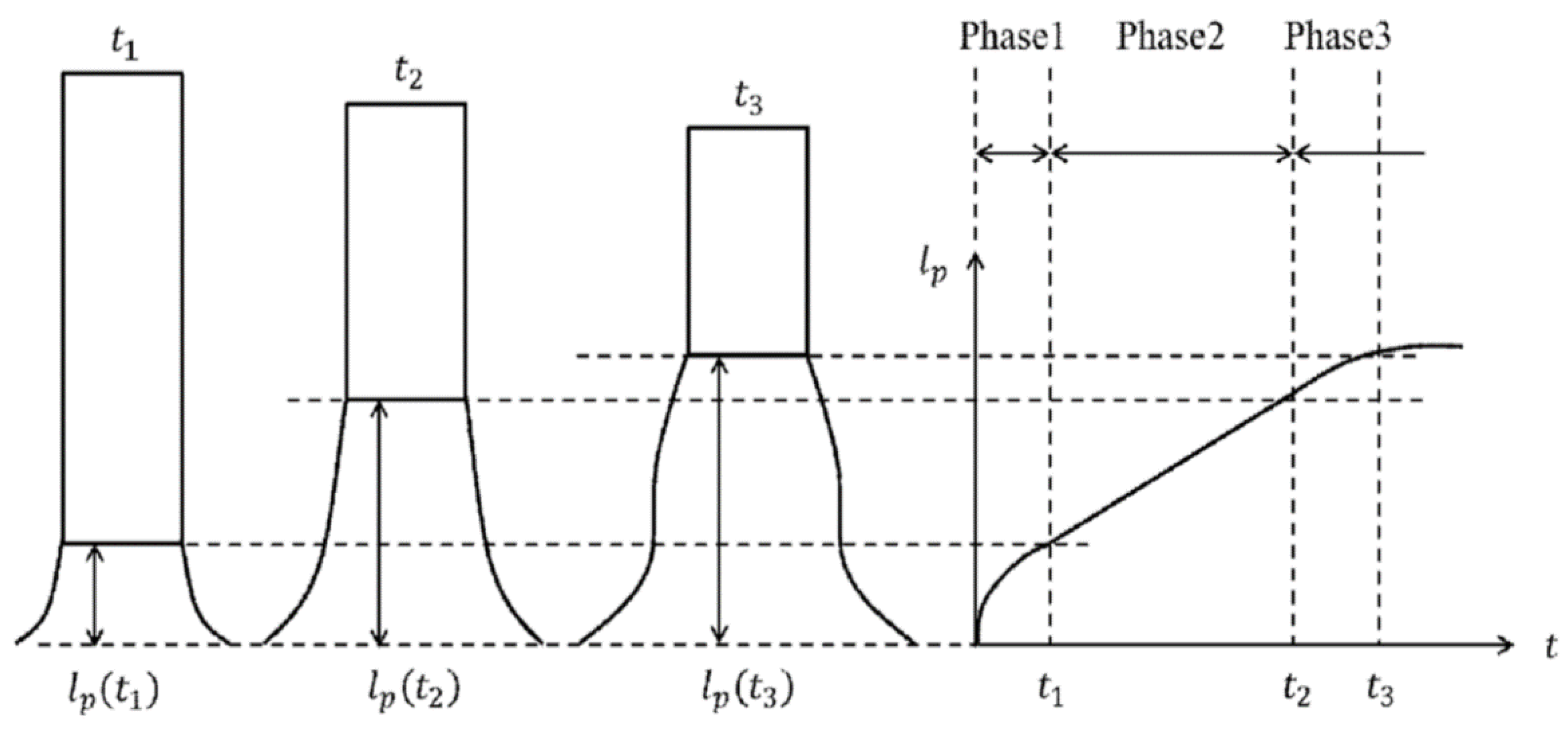
Jones et al. [10] have proposed that the deformation behavior in the Taylor impact test can be divided into three phases, depending on the position of the plastic wave front in the specimen. The details of the three phases proposed by Jones et al. [10] are expressed below. Figure 1 shows the schematic drawing of the three phases during deformation. In this figure, is length of a plastically-deformed region. Here, the period from the start of deformation to the time t1 is referred to as the phase 1, the period from the time t1 to t2 is referred to as phase 2, and the period after the time t2 is referred to as phase 3. As shown in Figure 1, Jones et al. [10] assumed that the phase 1 was nonlinear with respect to the time immediately after the impact. In addition, phase 2 represents a time period in which the plastic wave front is moving linearly with respect to time. The moving velocity of the plastic wave front is constant in this phase. After that, the particle velocity of the specimen becomes 0. Therefore, the region where the moving velocity of the plastic wave front approaches null can be considered to be phase 3. However, Jones et al. [10] provides no clear descriptions of the behavior of the specimen at each of these phases, the transition times t1 and t2, as well as its conditions. Focusing on phase 2, it is assumed that becomes almost constant. Additionally, can be measured by the difference in the outline of the deformed specimen at a different elapsed time.
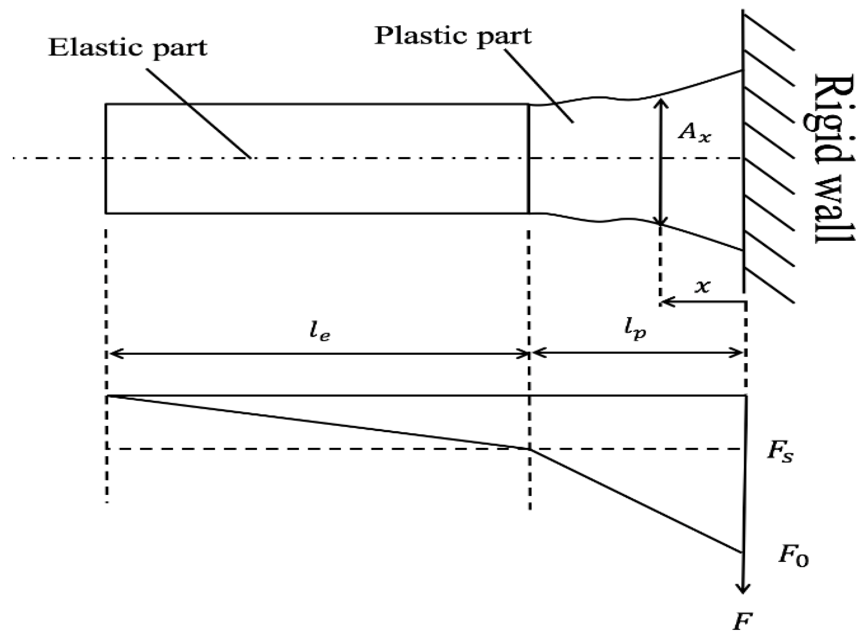
According to an inertia effect in the axial direction of the specimen, it is be realized that the internal force is distributed along with the axial direction of a specimen. Figure 2 shows the schematic drawing of the deformed specimen, and the axial distribution of the internal force. As shown in this figure, the linear distribution of the internal force in each region is assumed here. Hereafter, both regions are called the elastic part and the plastic part. Both and can be measured from the deformed profile of the specimen at an arbitrary time.
Based on the above assumptions, the distribution of the internal force can be calculated. The distribution of the axial internal force in the plastically-deformed and elastically-deformed regions of the specimen can be obtained through the following equations, which are expressed as a ratio between the internal force that is computed by the above assumption, and the current cross-sectional area:
Here, and denote the external force at an impact face of the specimen and the position from an origin at the impact end of the specimen. The true normal stress distribution of the specimen in the plastically- and elastically-deformed regions can be obtained through the following equations, which are expressed as a ratio between the internal force, computed by the above equation and the current cross-sectional area:
House et al. [19] introduces a high-speed camera for the first time, and conducts the Taylor impact test using oxygen-free copper to measure the shape of the specimen during deformation. In this study, the axial strain is calculated at each position in the axial direction of the specimen from the specimen shape under deformation. According to their method with assumptions of constant volume during plastic deformation and the dominance of plastic deformation, the axial strain can be calculated as:
Here, denotes the current cross-sectional area of the specimen at a position .
2.2. The Hardening Law to Nonlinear Strain Rate Sensitivity for the Finite Element Simulation
In order to simulate realistic deformation behavior, a selection of the hardening law, which indicates a relationship between the uniaxial stress, temperature, strain rate, and strain is quite important. Among the various hardening laws proposed in the past, there are three representative models. Firstly, the power-law model can be expressed as:
Here, , , , , and respectively mean the equivalent stress, the equivalent plastic strain, Young’s modulus, work-hardening exponent, and a material constant. The Ramberg-Osgood model [20] is applicable by adding the term of elastic strain into Equation (5), and is widely used for simulating the deformation behavior of major metallic materials. However, expressing the strain rate sensitivity as well as temperature dependency is quite tough, because strain rate and temperature are not included into the model. Several efforts on its extension are made; however, it can be said that a reliable and unified model is not found up to now.
Secondary, the hardening law proposed by Johnson and Cook [18] is frequently used as expressed in:
Here, , , , , and denote the equivalent plastic strain rate, the reference strain rate, the temperature of the material, the room temperature, and the melting temperature of the material, respectively. The parameters and are respectively the yield stress and the work hardening coefficient at the strain rate of and the temperature of . The parameter expresses the effect of thermal softening behaviour. The parameter indicates the coefficient of strain rate sensitivity. This model has already implemented into a lot of commercial FE codes because of its usability, as well as the availability of identified parameters in the model for various kinds of materials.
However, it is common that Equations (5) and (6) are empirical and phenomenological. In addition, it is not based on any underlying physics such as a thermal activation process, based on the dislocation theory. Thirdly, more physically-based models, for example, the model proposed by Zerilli and Armstrong [21] for fcc metals, can more legitimately be extrapolated, as expressed in:
Here, is the average grain size, and to are parameters. The second term inside the exponential function indicates the rate sensitivity. This term also depends on the temperature. However, it is quite hard to say that all three representative model can express the nonlinear rate sensitivity of materials, which appears especially at higher strain rate.
On the other hand, Allen et al. [14] proposed a nonlinear hardening model with respect to the strain rate, expressed as the following equation:
Here, the parameter indicates the exponent of strain rate sensitivity. This model is quite similar to the Johnson-Cook model expressed in Equation (6). The difference is the second bracket on the right-hand side to show the rate sensitivity. The rate sensitivity of the stress becomes nonlinear with respect to the logarithmic strain rate.
Like the work done by Iwamoto and Yokoyama [16], the selection of the hardening model was not a major target of this paper. In this research work, the nonlinear hardening model proposed by Allen et al. [14] expressed in Equation (8) is adopted for the finite element simulation of the modified Taylor impact test, because it can be used at the high strain rate to express nonlinear behavior with respect to the strain rate. In addition, the capability of the model is quite higher since only small changes from frequently-used Johnson-Cook model [18] in Equation (6) are sufficient.
2.3. A Removing Method of the Frictional Effect in Impact Compressive Tests Based on the SHPB Technique
In the past, it has been reported that the friction and radial inertia in the impact test based on SHPB method have an effect on the stress during the deformation [16]. Therefore, it is necessary to consider the relationship between the friction coefficient and slenderness ratio:
Here, , , , , , and denote modified value of stress, measured stress, increment value of stress due to friction, Poisson’s ratio, friction coefficient, and the slenderness ratio, respectively. Kii et al. [17] attempt to reduce the friction effect without any corrections of stress value by using a hollow specimen. In order to perform finite element analyses to show an effectiveness of hollow specimens, they also propose a method to correct the value of stress based on the above Equation (9) to identify the parameters in Johnson-Cook hardening law. In their method, , which means the true value of stress in the material, should be constant with respect to at constant values of and . In order to remove the frictional effect based on Equation (9), compressive tests using specimens with various are carried out. Then, calculated by Equation (9) with respect to is plotted against , and the linear approximate curve at the various values of are drawn. When the slope of the linear curve becomes almost zero, both and can be identified at the same time. As a result of both quasi-static and impact tests, the slope between the slenderness ratio and stress at a certain level of strain can be obtained.
3. Experimental Methods
3.1. Material and Specimen
The specimen was made of A1070, which is a pure aluminum under the Japan Industrial Standard (JIS). The shape of the specimen for the quasi-static test and impact test at 10−3 s−1 was a cylinder 14 mm in diameter. A circular plate with 3.6 mm in diameter for the impact test at 104 s−1 was used. From Equation (9), it can be seen that the slenderness ratio would also have an effect on the stress; therefore, the same value of slenderness ratio in specimens was used in both the quasi-static and impact tests. In order to remove the frictional effect based on Equation (9), the length or the thickness of the specimens was controlled to obtain the various slenderness ratios of 0.5, 1.0, 1.5, and 2.0 in the case of the quasi-static tests, and 0.4, 0.5, 0.7, and 1.0 in the case of the impact tests. All the specimens were annealed in a vacuum at 623 K for 1 h.
3.2. Quasi-Static and Impact Compressive Tests at Different Strain Rates and Temperatures
Quasi-static compressive tests were conducted by a material testing machine (Shimadzu AG-250 kN, Shimadzu corporation, Kyoto, Japan) with lubricant of MoS2. In order to determine the friction coefficient for quasi-static, the tests were conducted at room temperature for 10−3 s−1 of the strain rate. Next, the strain rate to measure the rate sensitivity in the stress-strain curves was set to 10−1, 10−2, and 10−3 s−1, and the test temperature was the room temperature. Then, it is carried out at 373, 473, and 573 K under 10−3 s−1 of the strain rate to obtain the temperature dependency in the stress-strain curves. Because the thermal energy was released to the outside faster than the speed of deformation during the quasi-static test, the temperature rise of the specimen could be vanished. After the quasi-static test to measure the elastic properties by using two rosette gauges, Young’s modulus was 67 GPa and Poisson’s ratio was 0.35.
It was shown that the stress-strain curve for the strain rate higher than 102–104 s−1 could be measured by using the SHPB technique with a thin cylindrical specimen [22]. The conventional size of the impact testing apparatus based on the SHPB method with 16 mm in diameter of the bars [23] was used to measure not only the stress-strain curve, but also the friction coefficient at the strain rate of 103 s−1. However, with the decrease in the diameter ratio of the specimen and the pressure bar to achieve the strain rate of 104 s−1, the punching or the indentation displacement [13] was increased. Consequently, it was difficult to measure the stress-strain curve accurately because of the effect of the punching displacement [13]. In order to obtain the stress-strain curve at a higher strain rate over 104 s−1, the impact compressive test was conducted by using the miniature testing apparatus, based on the SHPB method. Figure 3 shows the schematic illustration on the outline of used apparatus. The material of the striker bar and the pressure bars was SUJ2, which was bearing steel in the JIS standard, the lengths of the striker, input, and output bars were 150 mm, 400 mm, and 400 mm respectively. The diameter of the bars is 4 mm. The validity of the compressive tests obtained from the miniaturized testing apparatus, based on the SHPB method was discussed by comparing with the result that was obtained from the conventional size of the testing apparatus, based on the SHPB method [23] at a similar strain rate.
4. Finite Element Simulation of the Modified Taylor Impact Test
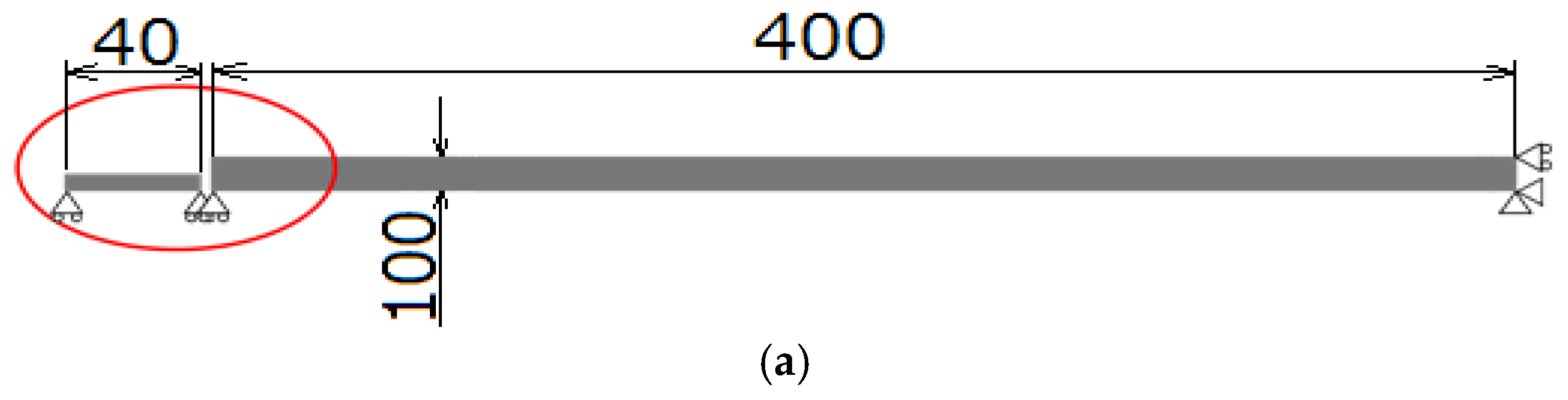
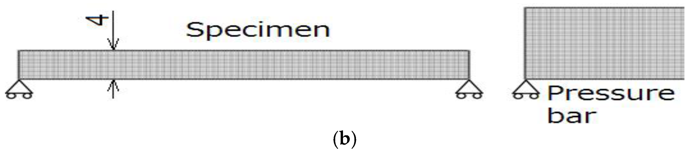
By using a commercial finite element software MSC Marc 2014 (Version 2014, MSC Software corporation, Los Angels, CA, USA), the finite element analyses of the modified Taylor impact test were performed at the initial velocities of the specimen, at 154 m/s. The finite element model is shown as Figure 4. As shown in Figure 4a, the specimen and the pressure bar were modelled as axisymmetric bodies. The shape of specimen was a cylinder 8 mm in diameter and 40 mm in length. The shape and dimensions were typical [12]. To measure the external force, the Hopkinson pressure bar was used in the apparatus of the Taylor impact test to replace the rigid wall. On the interface between the specimen and the stress bar, a hard contact condition with the kinematic friction was only considered, and its coefficient was set to the values that were determined later, based on Equation (9). The finite element used here was a four nodes bi-linear axisymmetric element. The numbers of elements and nodes were 4000 and 4221 respectively for the specimen, and 100,000 and 102,051 respectively for the pressure bar. Julien et al. [12] chose the Arbitrary Lagrangian-Eulerian (ALE) formulation to simulate the Taylor impact test of brass material in a three-dimensional space because the finite element (FE) meshes were extremely distorted around the contact region. The FE discretization in the present study was uniform, but the mesh size of 200 μm was small, as shown in Figure 4b, and the remeshing option was used to reduce such difficulties related to the distortion. It must be noted that, as explained above in Figure 1, excessive deformation of the specimen in the Phase 3 reduced the applicability of this method. Thus, the extremely huge deformed region induced errors, even though the stress and the strain in the region was precisely predicted. Like the compressive test, the specimen was assumed to be made of A1070. The pressure bar of 200 mm in diameter and 400 mm in length was assumed to be made of SUJ2. On the assumption of the actual experiment, the incident stress wave of the Hopkinson bar by generating an impacted specimen was captured. The pressure bar was assumed to be an isotropic linear elastic body with 7900 kg/m3 of the density, 209 GPa of Young’s modulus and 0.3 of the Poisson’s ratio. The density of the specimen was set to 2700 kg/m3 from the nominal value, based on a catalogue of pure aluminum. Unfortunately, the nonlinear hardening model in Equation (8) has not been implemented into any major commercial software, including MSC Marc 2014. Thus, it was implemented by using the user-subroutine named “WKLDP”.
On MSC Marc 2014, the analysis class chosen was Thermal/Structural, and the large strain option was checked. For the post-processes, the deformed profiles of the specimen were output at several points in elapsed time to obtain , , and in Equations (1), (3), and (4). The “historyplot” option was chosen to calculate in Equation (1). By combining the axial stress and strain at a certain time, the stress-strain curve could be obtained. Additionally, for a comparison with the axial stress and strain calculated by the deformed profiles, the “pathplot” option was also used to draw the axial stress and strain, along with the central axis of the specimen from their contour data.
5. Results and Discussions
5.1. Compressive Test from Quasi-Static to Impact Range
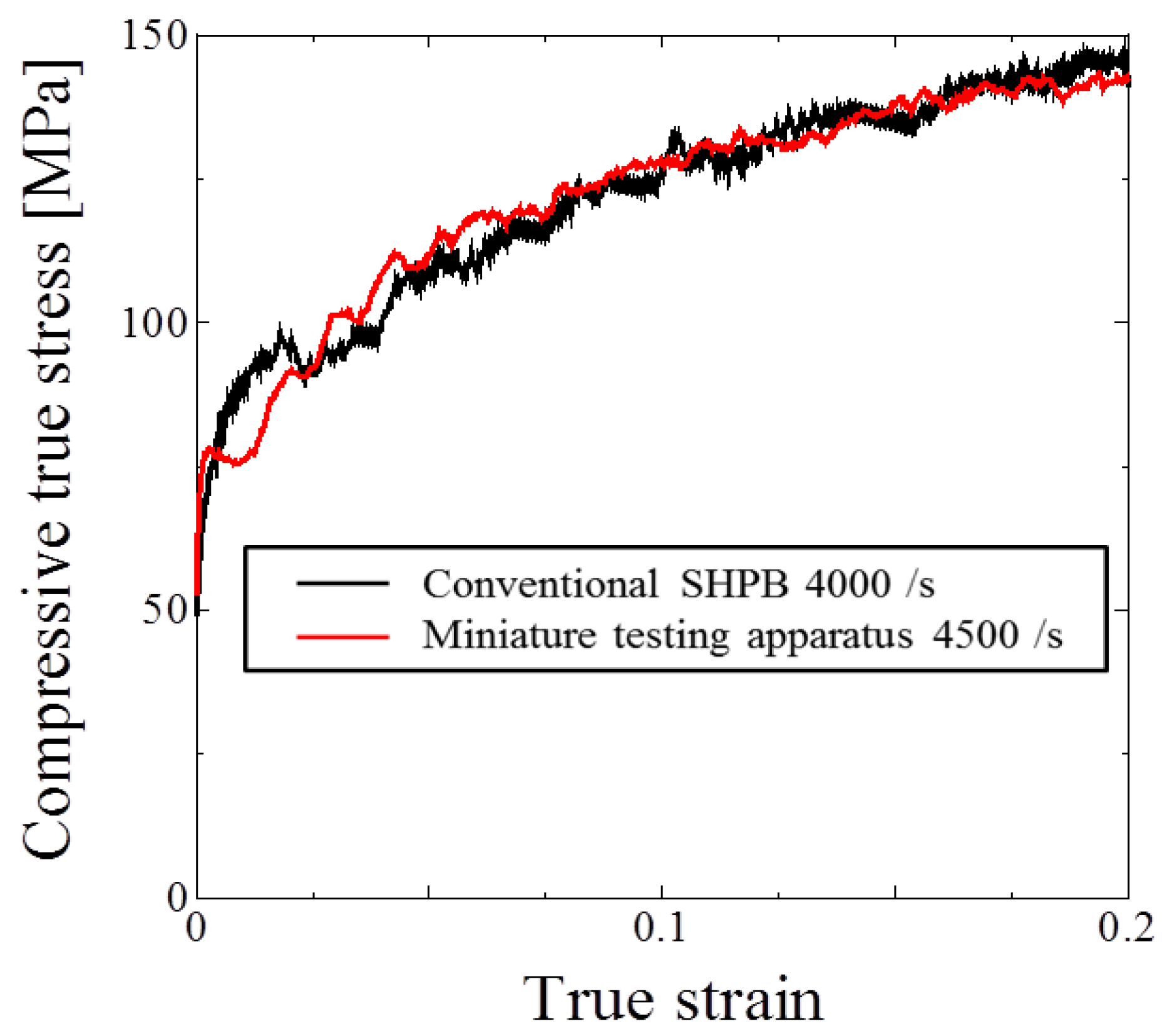
First of all, the validity of the impact test by the miniature impact testing apparatus was confirmed. Figure 5 shows the stress-strain curve obtained by setting the almost similar value of strain rate with the testing apparatus based on the SHPB method, with the bars being 16mm in diameter. From this figure, it can be found that the stress-strain curve obtained from the miniature apparatus almost coincided with the result of the conventional testing apparatus in the range of the target strain rate for this experiment. The strain rate obtained in both testing apparatuses was similar. From the above, it can be estimated that the miniaturized testing apparatus was valid. Additionally, it can also be seen that the size of the specimen had almost no effect on the stress-strain curve in the range of the strain rate, as 103 s−1.
Figure 6 shows the relationship between modified stress , calculated by Equation (9) for each friction coefficient and slenderness ratio obtained by (a) quasi-static and (b) impact tests. As performed by Kii et al. [17], the approximated linear curve was drawn for each of the plots of the conditions, based on Equation (9), and the slope of the curve was plotted against the friction coefficient. As per the results of an extrapolation when the slope becomes zero, the friction coefficient was determined as 0.18 for the quasi-static test, and 0.03 for the impact test, respectively. At the same time, the modified stress could be also determined, so that modified values were used to identify the parameter in the model.
In order to identify the parameters in the hardening laws, the least-square method or some other optimization technique is employed [2,24]. Here, the following identification method by a manual-like procedure was chosen. At first, in Equation (8) is set to the lowest strain rate as 10−3. By fitting the experimentally-obtained curve at and , , , and could be identified. Then, was determined from the experimental data at by changing . Finally, could be obtained from the experimental data of the stress for 0.1 of the strain at various strain rates. As a result of the procedure, all the identified parameters in Equation (8) are shown in Table 1.
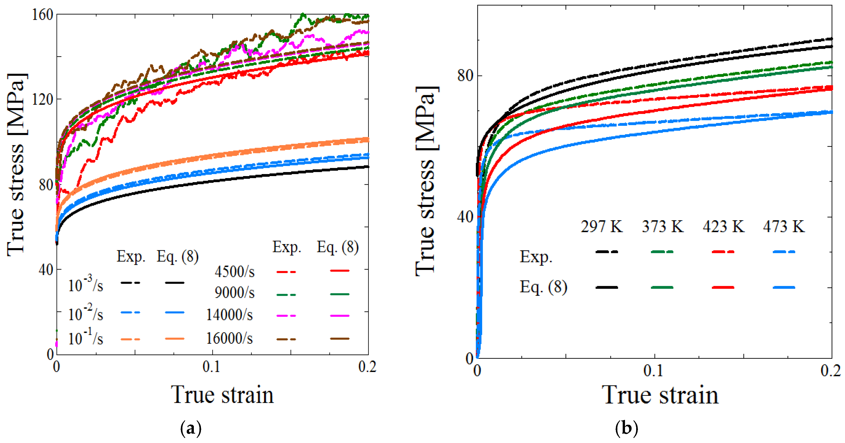
Figure 7 shows the stress-strain relationship at various (a) strain rate and (b) temperature. In the figure, the experiment results with the modified stress are shown by dashed lines, and the results drawn by calculating the model in Equation (8) are shown by solid lines. From this figure, it can be understood that the experimental results and the results by model by Allen et al. [14] were in good agreement in the small strain range of less than 0.1. From this result, it was found that the model could express the rate-sensitive and temperature-dependent deformation behavior accurately at a strain rate range of around 104 s−1.
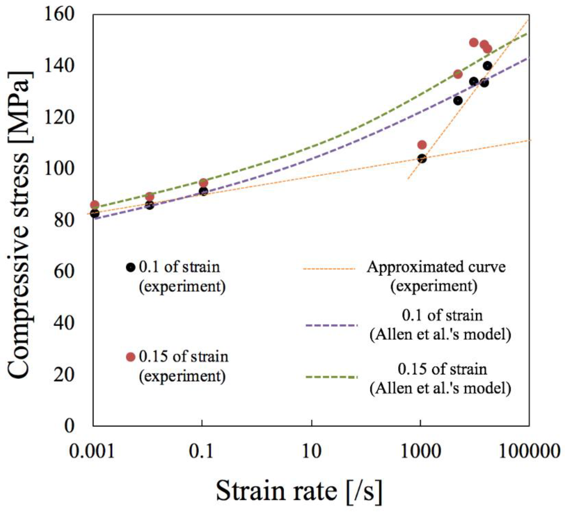
Figure 8 shows the relationship between the stress and strain rate for true axial strain of 0.1 and 0.15, obtained by experimental methods, and the model proposed by Allen et al. [14]. It has been reported that pure aluminum, which is the face-centered cubic structure, shows a steep rise in stress at the strain rate of about 5000 s−1 from the past study [15]. Furthermore, the stress becomes nonlinear with respect to the strain rate. As shown in this figure, it was understood that the stress value obtained from the miniaturized testing apparatus showed a sharp rise around the strain rate of 103 s−1, and the nonlinearity could be also confirmed, as in the previous studies [15]. From these results, the nonlinear strain rate sensitivity of the material could be measured correctly by using the miniature testing apparatus. In addition, from the results obtained by the model proposed by Allen et al. [14], the stress value rose sharply at a strain rate of 102 s−1. This fairly good agreement could be confirmed with the results that were obtained by experimental methods, at a strain rate over 104 s−1. Overall, the model proposed by Allen et al. [14] could be used at a super high strain rate.
5.2. Computation of the Modified Taylor Impact Test by FEM
Using finite element analysis, the modified Taylor impact test proposed here was performed with an initial impact speed of the specimen at 154 m/s. As a result, the above-mentioned calculation method of a stress-strain curve explained in Section 2.1 was studied. Using the time history of the external force obtained from the pressure bar, the velocity at the free end of the specimen, the time history of the deformed profile in the specimen, at each time, the stress-strain curve was calculated by the method shown previously. The stress-strain curve obtained in the analysis was compared with the curve that was calculated by the model expressed in Equation (8), and the validity of the obtained stress-strain curve by the above-mentioned method was investigated.
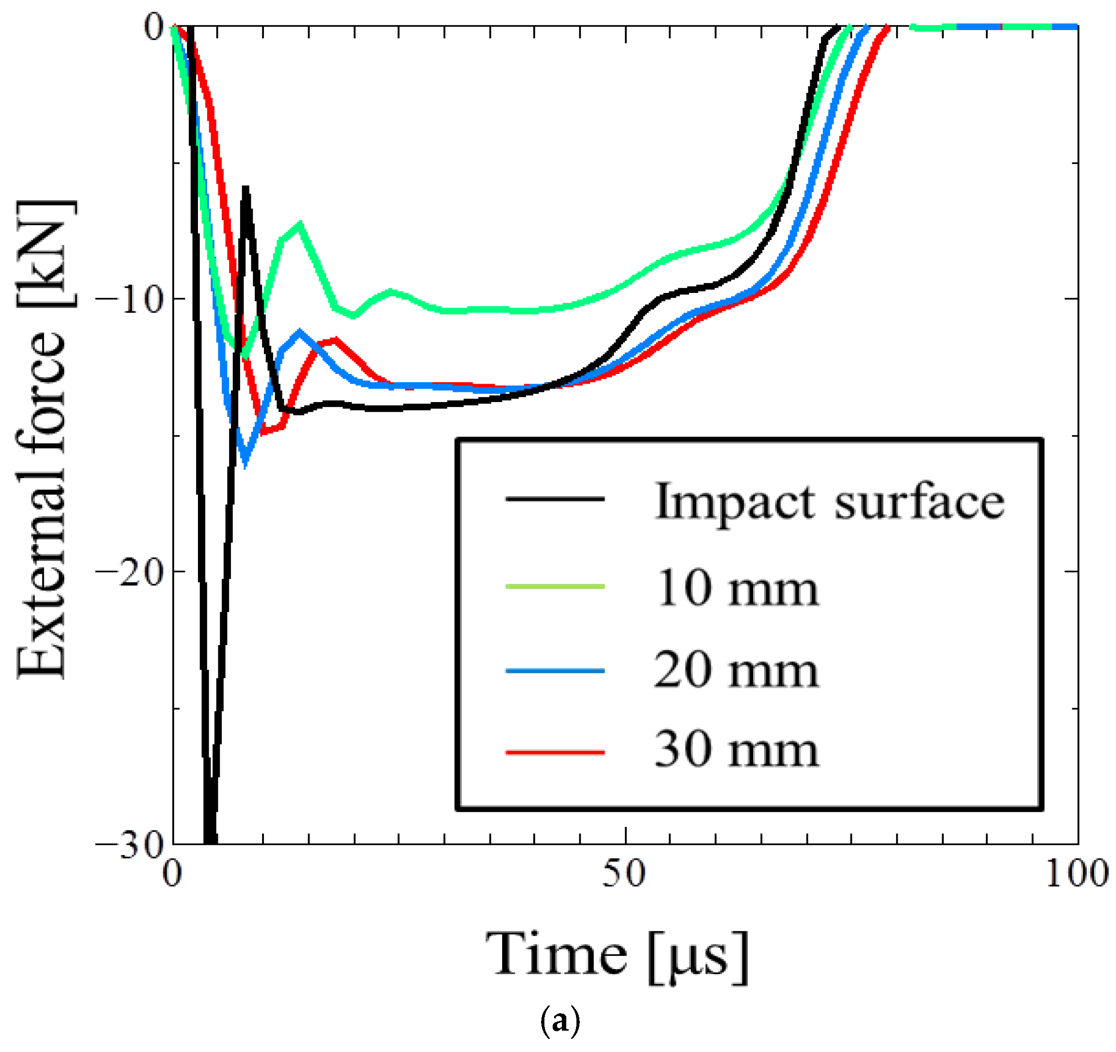
Figure 9 shows (a) the time history of the external force obtained by finite element analysis (FEA) at the positions of 10, 20, and 30 mm away from the impact surface as the origin, and (b) a contour plot of axial stress during the impact of the specimen at 20 μs of time elapsed. In Figure 9a, the black line shows the time history of the reaction force by a contact acting on the impact surface of the specimen, and the green, blue, and red lines represent the time histories of the external force as measured on the surface of the pressure bar at 10, 20, and 30 mm from the impact surface, respectively. From this figure, it was found that the time history of the external force at the position 20 mm or more away from the impact surface could be accurately measured, excluding a spike generated immediately after the impact. In addition, as shown in Figure 9b, the one-dimensional stress wave propagation has not been achieved in the region within 10 mm from the impact surface. From the above results, it was considered that an accurate measurement was difficult when the stress wave was measured near the impact surface. In the finite element analysis, it was assumed that the specimen completely impacted, with the center of the pressure bar. However, when actually conducting this proposed method based on the Taylor impact test, a statistical variation in a position on the impact surface, where the specimen collides with the pressure bar easily occurs. Therefore, it is sufficiently conceivable that the region in the three-dimensional stress wave propagation in the pressure bar becomes larger than the region obtained by the FEA, as shown in Figure 9b. Therefore, in order to reliably measure the time history of the external force, the measurement position is determined to be 30 mm from the impact surface.
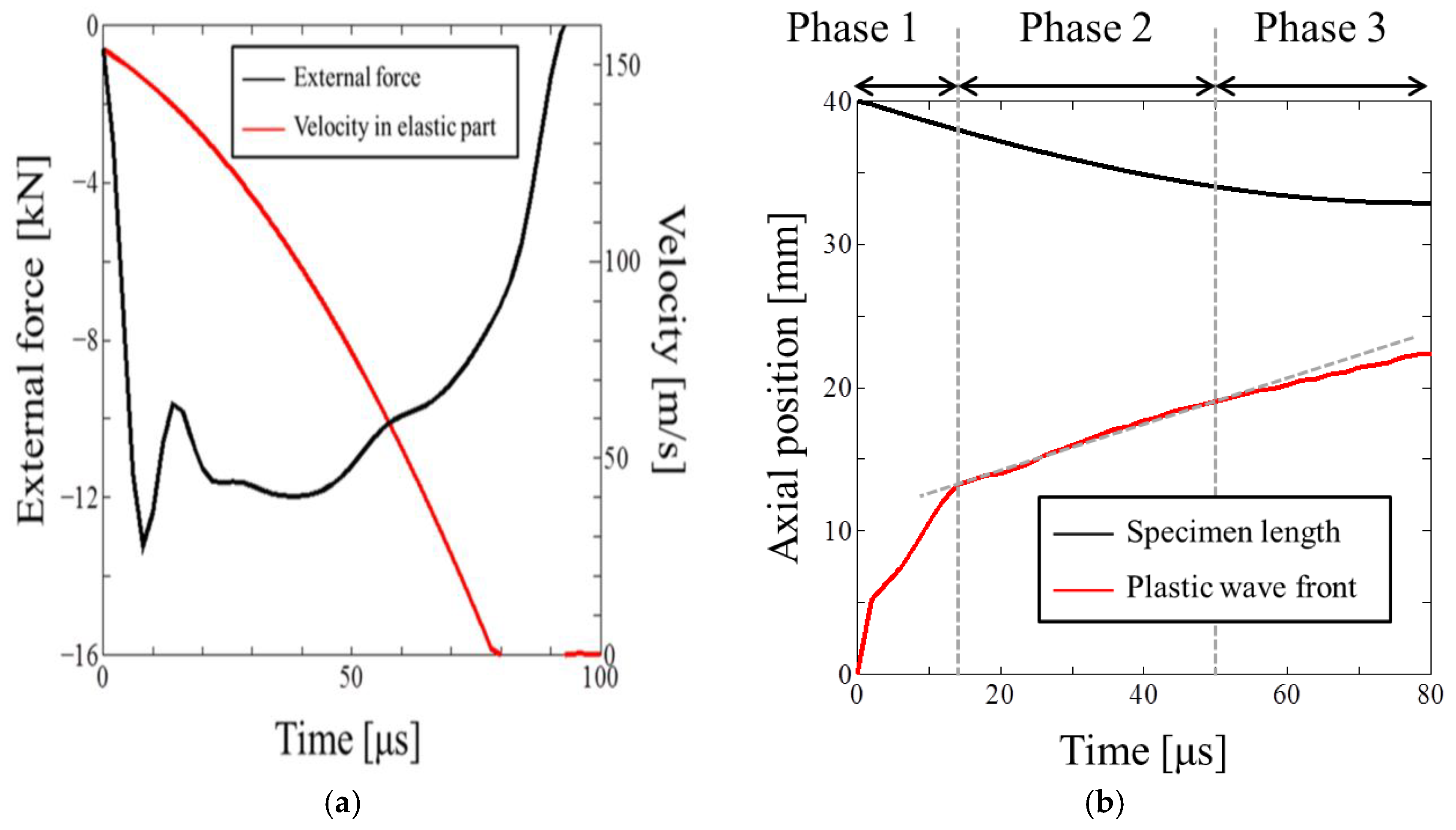
Figure 10 shows the time histories of (a) the external force obtained from the pressure bar and the velocity at the free end of the specimen, and (b) the length of the specimen and the distance of the plastic wave front from the impact surface. In Figure 10a, the black and red lines represent the external force and the velocity at the free end of the specimen. In Figure 10b, the black and red lines represent the length of the specimen and the position of the plastic wave front, respectively. As shown in Figure 10a, the duration of the external force was about 92 μs, and the time to decrease to 0 m/s for the velocity at the free end of the specimen is about 78 μs. From this result, it was found that the impact state continued for about 14 μs after the velocity at the free end of the specimen became 0 m/s. Just after the velocity at the free end of the specimen achieves 0 m/s, the length of the specimen becomes about 33 mm, as shown in Figure 10b. From this length, the time period to reciprocate the elastic stress wave once in the specimen was calculated as 13.2 μs, which was the time to decrease the external force rapidly after the velocity at the end of the specimen to become 0 m/s. This almost coincided with the time that was required for the history to decrease to zero. Therefore, it can be inferred that this phenomenon was due to the fact that it takes time for the unloading wave to reciprocate in the test piece after the particle velocity at the end of the specimen becomes zero. Since the duration of the time history of external force is the time during which the pressure bar and the specimen are in contact, the duration of the time history of the external force was the duration of this test. Moreover, as shown in Figure 10b, the position of the plastic wave front changed nonlinearly from the start of the impact to about 14 μs, then it showed a linear change, and its change became nonlinear again after about 50 μs. This represented the transition time from phase 1 to 2 and from 2 to 3, respectively, as described before. In this case, and were about 14 and 50 μs. in Equation (1) could be captured by the slope of the red line in Figure 10a, from to .
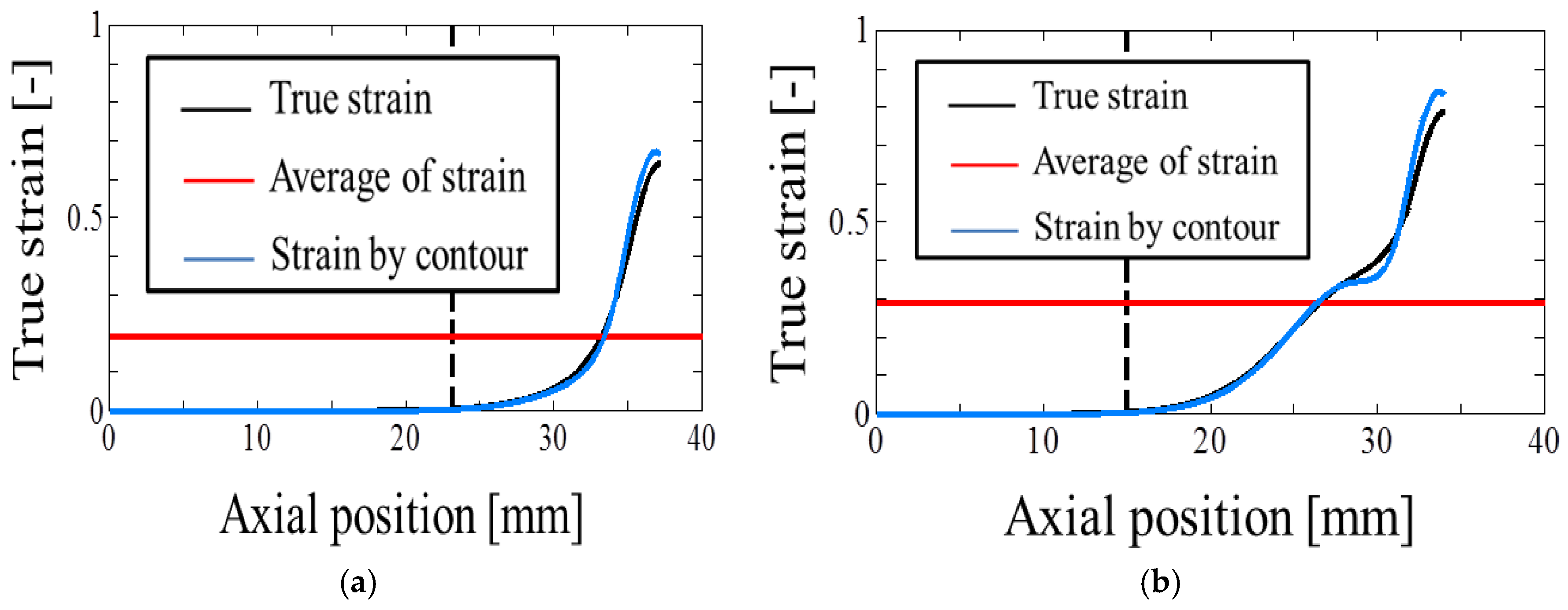
Figure 11 shows the distribution of axial strain calculated from various methods at (a) 20 and (b) 50 μs of elapsed time since the impact. In the figure, the black line shows the results calculated by Equation (4) with the outline of the deformed specimen, the blue line shows the results obtained from the contour plot of FEA, the red line shows the average strain of the plastic part, and the dashed line shows the position of the plastic wave front. From this figure, the distribution of axial strain calculated by Equation (4) was in good agreement with that obtained from the contour plot, and it was evaluated that the calculated distribution by Equation (4) was appropriate. In addition, an increase in a quite highly deformed region, as similar to the buckling at 50 μs, could be observed locally.
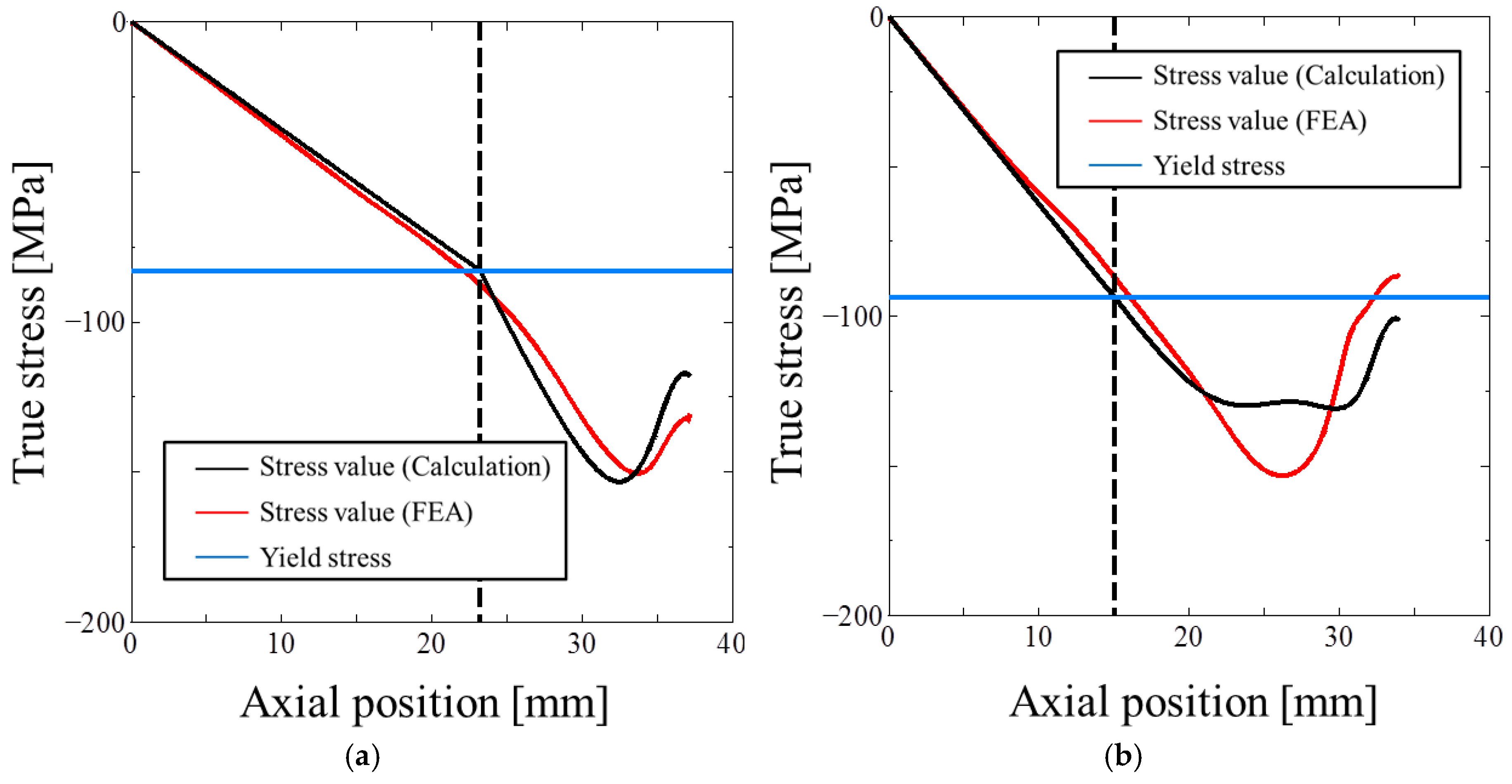
Figure 12 shows the distribution of axial stress in the specimen at (a) 20 and (b) 50 μs of elapsed time since the impact. In this figure, the black line is the calculated result from the bi-linear approximation by Equation (3), the red line is the obtained result from a contour map by FEA, the blue line is the stress at the interface calculated by Equation (1), and the dashed line is the position of the plastic wave front, respectively. From this figure, the stress at the interface calculated by Equation (1) and the stress value at the plastic wave front obtained by the FEA agreed well. This means that in phase 2, the calculation of stress distribution by bi-linear approximation was applicable. Also, in the time after 20 μs, the stress value decreased in the region with the higher value of axial strain near the impact surface. The precision for predicting the distribution was much higher at 20 μs. Therefore, a good measurement could be obtained at a time close to .
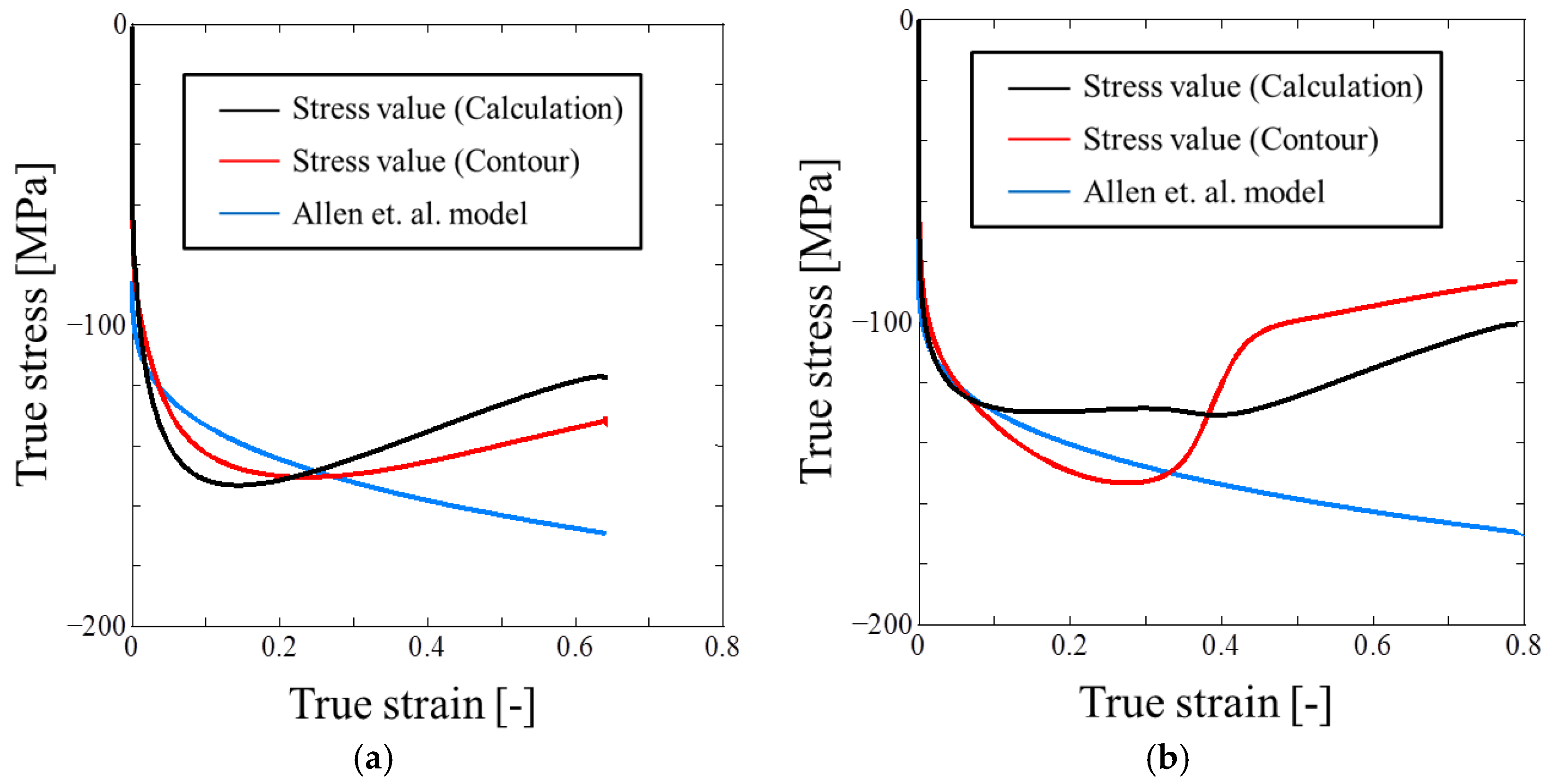
Figure 13 shows the stress-strain curves at each elapsed time. In the figure, the black line is the calculated curve from the bi-linear approximation, the red line is the obtained curve from FEA, and the blue line is directly calculated from the model by Allen et al. [14] in Equation (8). From this figure (a), the stress-strain curves obtained by the bi-linear approximation and the contour plot showed good agreement at 20 μs, when it could be seen that the approximation of the stress distribution was possible, as shown in Figure 13. However, it is understood that the difference from the curve calculated by the model gets larger as the strain increases. Since it is conceivable that the starting time of plastic deformation everywhere in the specimen is also different, it is possible that the stress value becomes low in the higher strain region located around the impact surface. On the other hand, in the smaller region of strain less than 0.05, the curve obtained by these three methods showed fairly good agreement at 50 μs. From this figure, it was found that better measurements of the curve could be realized at a time close to , when the plastic wave sufficiently propagated at a constant velocity.
Of course, this method was applicable when the loading only occurred in the entire region of specimens. The deformation history at different material points must be considered carefully if the distribution of stress and strain is linked together. On the other hand, it is difficult to establish the method of the calculation of the strain rate. Therefore, it was necessary to establish the calculation method with a higher precision of the stress-strain curve and strain rate, by using not only the theory of stress wave propagation, but also the laws of physics from the deformation of the specimens, as well as the time history of the external force.
6. Concluding Remarks
In this study, to measure the stress-strain curve at only one single trial of the Taylor impact test, its modification method was newly proposed. In the method, a measurement of the external force by the Hopkinson pressure bar, an assumption of bi-linear distribution of an internal force and a combination between the distributions of the axial stress and strain at a certain time, were employed. Before the feasibility of the proposed method was studied, at first, the quasi-static and the impact tests at various strain rates and temperatures were conducted to identify the parameters in a nonlinear rate sensitive hardening law. Then, the hardening law with the identified parameters was implemented into the commercial code through the user-subroutine. Next, a series of finite element simulations was performed by using the implemented model to confirm the feasibility. The following results were obtained.
- It is possible to obtain a valid stress-strain curve at only one single trial of the Taylor impact test.
- In the Phase 2, the distribution of the axial internal force can be approximated bi-linearly with respect to the axial position of the specimen.
- It can be observed that the axial stress decreases mainly in the region of higher strain.
- The choice of elapsed time during Phase 2 is quite important, in order to obtain the correct stress-strain curve.
At present, the strain rate cannot be calculated and stress-strain curve can be obtained at smaller strains of less than 0.1. Further modifications of this method are necessary to solve the above issues.
Author Contributions
C.G. and T.I. conceived and designed the experiments; C.G. performed the experiments; C.G. and T.I. analyzed the data; T.I. contributed reagents/materials/analysis tools; C.G. and T.I. wrote the paper.
Funding
This work was funded by JSPS KAKENHI, Grant Number JP16K14504.
Acknowledgments
We would like to thank Fumiaki Iwasaki of Nippon Light Metals Co, Ltd. for his assistance with the experimental investigation.
Conflicts of Interest
The authors declare no conflict of interest.
References
- Taylor, G. The use of flat-ended projectiles for determining dynamic yield stress. Proc. R. Soc. Lond. Ser. A 1948, 194, 289–299. [Google Scholar] [CrossRef]
- Piao, M.; Huh, H.; Lee, I.; Ahn, K.; Kim, H.; Park, L. Characterization of flow stress at ultra-high strain rates by proper extrapolation with Taylor impact tests. Int. J. Impact Eng. 2016, 91, 142–157. [Google Scholar] [CrossRef]
- Sarva, S.; Mulliken, A.D.; Boyce, M.C. Mechanics of Taylor impact testing of polycarbonate. Int. J. Solids Struct. 2007, 44, 2381–2400. [Google Scholar] [CrossRef]
- Millett, J.C.F.; Bourne, N.K.; Stevens, G.S. Taylor impact of polyether ether ketone. Int. J. Impact Eng. 2006, 32, 1086–1094. [Google Scholar] [CrossRef]
- Lopanikov, S.L.; Gama, B.A.; Haque, M.J.; Krauthauser, C.; Gillesspie, J.W.; Guden, M., Jr.; Hall, I.W. Dynamics of metal foam deformation during Taylor cylinder-Hopkinson bar impact experiment. Compos. Struct. 2003, 61, 61–71. [Google Scholar] [CrossRef]
- Yahaya, M.A.; Ruan, D.; Lu, G.; Dargusch, M.S.; Yu, T.X. Selection of densification strain to predict dynamic crushing stress at high impact velocity of ALPORAS aluminium foam. Key Eng. Mater. 2015, 626, 383–388. [Google Scholar] [CrossRef]
- Wilkins, M.L.; Guinan, M.W. Impact of cylinders on a rigid boundary. J. Appl. Phys. 1973, 44, 1200–1206. [Google Scholar] [CrossRef]
- Mocko, W.; Janiszewski, J.; Radziejewska, J.; Grazka, M. Analysis of deformation history and damage initiation for 6082-T6 aluminium alloy loaded at classic and symmetric Taylor impact test conditions. Int. J. Impact Eng. 2015, 75, 203–213. [Google Scholar] [CrossRef]
- Forde, L.C.; Proud, W.G.; Walley, S.M. Symmetrical Taylor impact studies of copper. Proc. R. Soc. A 2009, 465, 769–790. [Google Scholar] [CrossRef] [Green Version]
- Jones, S.E.; Maudlin, P.J.; Foster, J.C., Jr. An engineering analysis of plastic wave propagation in the Taylor test. Int. J. Impact Eng. 1997, 19, 95–106. [Google Scholar] [CrossRef]
- Jones, S.E.; Drinkard, J.A.; Rule, W.K.; Wilson, L.L. An elementary theory for the Taylor impact test. Int. J. Impact Eng. 1998, 21, 1–13. [Google Scholar] [CrossRef]
- Julien, R.; Jankowiak, T.; Rusinek, A.; Wood, P. Taylor’s test technique for dynamic characterization of materials: Application to brass. Exp. Tech. 2016, 40, 347–355. [Google Scholar] [CrossRef]
- Safa, K.; Gary, G. Displacement correction for punching at a dynamically loaded bar end. Int. J. Impact Eng. 2010, 37, 371–384. [Google Scholar] [CrossRef] [Green Version]
- Allen, D.J.; Rule, W.K.; Jones, S.E. Optimizing material strength constants numerically extracted from Taylor impact data. Exp. Mech. 1997, 37, 333–338. [Google Scholar] [CrossRef]
- Sakino, K. Strain rate sensitivity of dynamic flow stress of FCC metals at very high strain rates. Transact. Jpn. Soc. Mech. Eng. Ser. A 1997, 63, 939–944. [Google Scholar] [CrossRef]
- Iwamoto, T.; Yokoyama, T. Effects of radial inertia and end friction in specimen geometry in split Hopkinson pressure bar tests: A computational study. Mech. Mater. 2012, 51, 97–109. [Google Scholar] [CrossRef]
- Kii, N.; Iwamoto, T.; Rusinek, A.; Jankowiak, T. A study on reduction of friction in impact compressive test based on the split Hopkinson pressure bar method by using a hollow specimen. Appl. Mech. Mater. 2014, 566, 548–553. [Google Scholar] [CrossRef]
- Johnson, G.R.; Cook, W.H. A constitutive model and data for metals subjected to large strains, high strain rates, and high temperatures. Proc. 7th Int. Sympo. Ballist. 1983, 541–547. Available online: https://ci.nii.ac.jp/naid/20000193157/ (accessed on 13 August 2018).
- House, J.W.; Aref, B.; Foster, J.C., Jr.; Gillis, P.P. Film data reduction from Taylor impact tests. J. Strain Anal. Eng. Des. 1999, 34, 337–345. [Google Scholar] [CrossRef]
- Ramberg, W.; Osgood, W.R. Description of Stress-Strain Curves by Three Parameters; Technical Note No. 902; National Advisory Committee for Aeronautics: Washington, DC, USA, 1943.
- Zerilli, F.J.; Armstrong, R.W. Dislocation-mechanics-based constitutive relations for material dynamics calculations. J. Appl. Phys. 1987, 61, 1816–1825. [Google Scholar] [CrossRef] [Green Version]
- Jia, D.; Ramesh, K.T. A rigorous assessment of the benefits of miniaturization in the Kolsky bar system. Exp. Mech. 2004, 44, 445–454. [Google Scholar] [CrossRef]
- Iwamoto, T.; Cherkaoui, M.; Sawa, T. A study on impact deformation and transformation behavior of TRIP steel by finite element simulation and experiment. Int. J. Mod. Phys. B 2008, 22, 5985–5990. [Google Scholar] [CrossRef]
- Iwamoto, T.; Kawagishi, Y.; Tsuta, T.; Morita, S. Identification of constitutive equation for TRIP steel and its application to improve mechanical properties. JSME Int. J. Ser. A 2001, 44, 443–452. [Google Scholar] [CrossRef]
Figure 1.
A schematic drawing of specimen at , , , and the time history of the wave front of the plastic region, to explain the partition of phase in the deformation behaviour of the specimen during the Taylor impact test.
Figure 1.
A schematic drawing of specimen at , , , and the time history of the wave front of the plastic region, to explain the partition of phase in the deformation behaviour of the specimen during the Taylor impact test.

Figure 2.
A schematic drawing of deformed specimen and axial distribution of internal force.

Figure 3.
A schematic illustration of established miniature split Hopkinson pressure bar (SHPB) testing apparatus.
Figure 3.
A schematic illustration of established miniature split Hopkinson pressure bar (SHPB) testing apparatus.
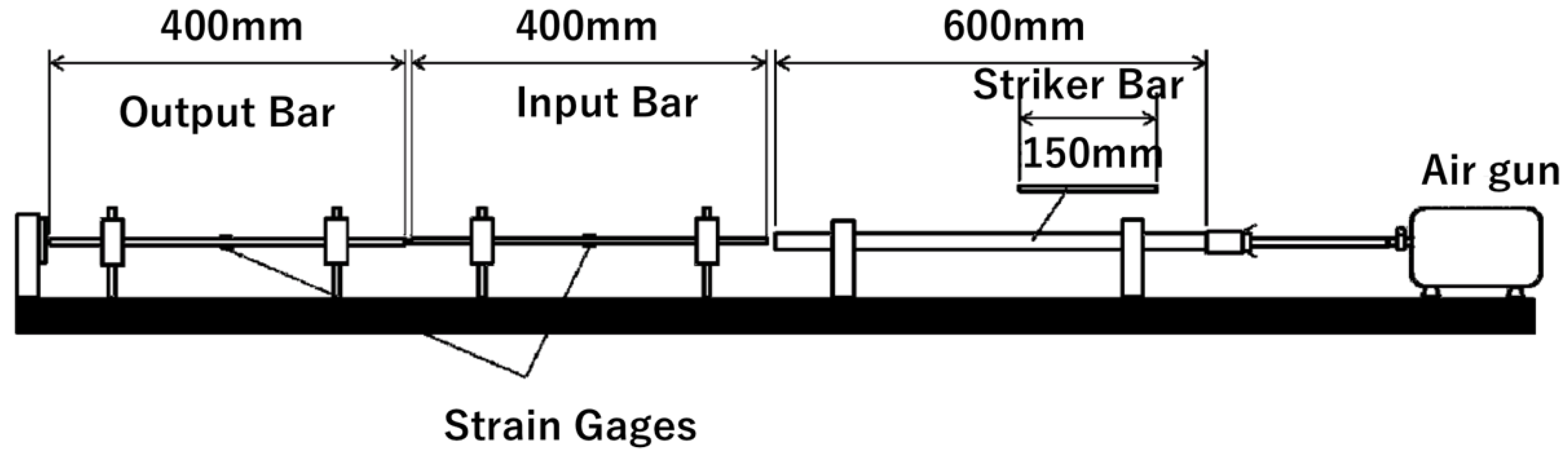
Figure 4.
The finite element model of the modified Taylor impact test using a pressure bar. (a) The whole view and (b) the magnified view around an interface between the specimen and the pressure bar, as shown in the red circle of the figure (a) (dimensions in mm).
Figure 4.
The finite element model of the modified Taylor impact test using a pressure bar. (a) The whole view and (b) the magnified view around an interface between the specimen and the pressure bar, as shown in the red circle of the figure (a) (dimensions in mm).


Figure 5.
A comparison between the stress-strain curves obtained by the conventional and miniature testing apparatuses.
Figure 5.
A comparison between the stress-strain curves obtained by the conventional and miniature testing apparatuses.

Figure 6.
The relationship between modified stress calculated by Equation (9) for each friction coefficient and slenderness ratio obtained by (a) quasi-static and (b) impact tests using an annealed specimen.
Figure 6.
The relationship between modified stress calculated by Equation (9) for each friction coefficient and slenderness ratio obtained by (a) quasi-static and (b) impact tests using an annealed specimen.

Figure 7.
Stress-strain curves obtained by a quasi-static and impact test at various temperatures and directly calculated by Equation (8). (a) At various strain rates; (b) At various temperatures.
Figure 7.
Stress-strain curves obtained by a quasi-static and impact test at various temperatures and directly calculated by Equation (8). (a) At various strain rates; (b) At various temperatures.

Figure 8.
Stress-strain rate relationship obtained by quasi-static to impact tests using the established miniature testing apparatus.
Figure 8.
Stress-strain rate relationship obtained by quasi-static to impact tests using the established miniature testing apparatus.

Figure 9.
Determination of a measuring position of external force from the impact surface. (a) Time history of the external force. (b) Contour of axial stress at 20 μs.
Figure 9.
Determination of a measuring position of external force from the impact surface. (a) Time history of the external force. (b) Contour of axial stress at 20 μs.

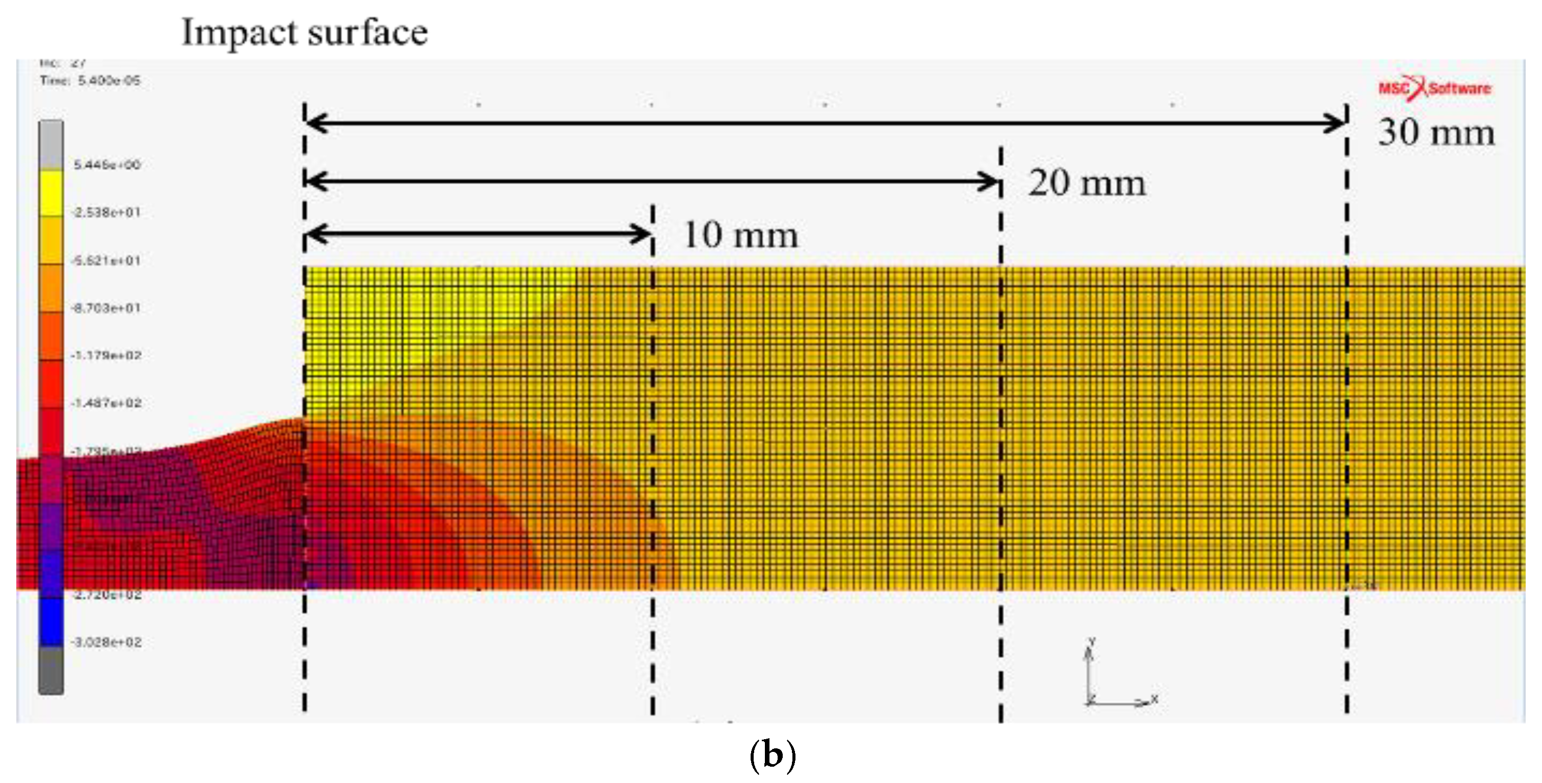
Figure 10.
Time histories of some important parameters in the specimen. (a) External force and velocity in the elastic part. (b) Length and position of the plastic wave front.
Figure 10.
Time histories of some important parameters in the specimen. (a) External force and velocity in the elastic part. (b) Length and position of the plastic wave front.

Figure 11.
Distribution of the true strain obtained by Equation (4), a contour as a result of FEA and average of strain at each elapsed time. (a) 20 μs; (b) 50 μs.
Figure 11.
Distribution of the true strain obtained by Equation (4), a contour as a result of FEA and average of strain at each elapsed time. (a) 20 μs; (b) 50 μs.

Figure 12.
Distribution of axial stress obtained by a bi-linear approximation using Equation (3), the FEA, and the calculated yield stress by Equation (1) at each elapsed time since the impact. (a) 20 μs, (b) 50 μs.
Figure 12.
Distribution of axial stress obtained by a bi-linear approximation using Equation (3), the FEA, and the calculated yield stress by Equation (1) at each elapsed time since the impact. (a) 20 μs, (b) 50 μs.

Figure 13.
Stress-strain curve at each elapsed time by combining Figure 11 and Figure 12. (a) 20 μs, (b) 50 μs.


Table 1.
The material parameters of the models by Allen et al. [14], determined by experimental results.
Table 1.
The material parameters of the models by Allen et al. [14], determined by experimental results.
| 49.7 | 60.6 | 0.282 | 0.001 | 0.0307 | 1.14 |
© 2018 by the authors. Licensee MDPI, Basel, Switzerland. This article is an open access article distributed under the terms and conditions of the Creative Commons Attribution (CC BY) license (http://creativecommons.org/licenses/by/4.0/).
Share and Cite
MDPI and ACS Style
Gao, C.; Iwamoto, T. Finite Element Analysis on a Newly-Modified Method for the Taylor Impact Test to Measure the Stress-Strain Curve by the Only Single Test Using Pure Aluminum. Metals 2018, 8, 642. https://doi.org/10.3390/met8080642
AMA Style
Gao C, Iwamoto T. Finite Element Analysis on a Newly-Modified Method for the Taylor Impact Test to Measure the Stress-Strain Curve by the Only Single Test Using Pure Aluminum. Metals. 2018; 8(8):642. https://doi.org/10.3390/met8080642
Chicago/Turabian StyleGao, Chong, and Takeshi Iwamoto. 2018. "Finite Element Analysis on a Newly-Modified Method for the Taylor Impact Test to Measure the Stress-Strain Curve by the Only Single Test Using Pure Aluminum" Metals 8, no. 8: 642. https://doi.org/10.3390/met8080642
Note that from the first issue of 2016, this journal uses article numbers instead of page numbers. See further details here.