1. Introduction
Flatness is a key quality indicator for cold-rolled steel strips [
1,
2], and the flatness roll is the core piece of detection equipment in a flatness measurement and control system [
3,
4,
5]. By coming into direct contact with the surface of the steel strip, the flatness roll can detect the tension distribution in the width direction of the steel strip and calculate the flatness distribution in real time. During detection, the steel strip fully covers the flatness roll and enables transmission. The roll surface not only bears periodic alternating loads from the steel strip but also experiences slipping and wear due to the different speeds between the strip and the roll [
6,
7].
Before leaving the factory, the whole-roll flatness roll is often subjected to surface heat treatment through electromagnetic induction quenching to strengthen the roll surface, resulting in a relatively thin martensitic hardened layer on the surface, while the original pearlitic structure in the core is retained. The depth of the hardened layer determines the service life of the flatness roll, and its uniformity affects the overall mechanical performance, while hardness is an important parameter for evaluating the wear resistance of the roll surface. Unlike the surface quenching process of work rolls [
8,
9], the whole-roll flatness roll has axial through-holes near the roll surface, where sensors are installed and subjected to high pre-tension, causing elastic deformation of the roll surface by tens of micrometers. This requires minimizing the depth of the hardened layer and ensuring its uniform distribution, so that the surface hardness and roll body toughness are coordinated to prevent cracking of the roll surface when the sensors are installed.
Many scholars have conducted detailed studies on electromagnetic induction quenching. Lu et al. [
10] used JIS SUJ2 steel as the material for induction quenching and studied the distribution of residual stress and residual austenite. The results showed that the microstructure of the specimen before induction quenching had a significant impact on the depth of the hardened layer, and the maximum residual compressive stress increased with the rise in austenitizing temperature. Derouiche et al. [
11] developed two data-driven models for the temperature–time evolution and austenite phase transformation during induction heating and created data-driven and hybrid models to predict hardness after quenching. Fang et al. [
12] used cold rolling and electromagnetic induction heating to manufacture gradient structures on AISI 316L stainless steel and studied the effect of surface softening on the fatigue behavior of AISI 316L stainless steel. Jian et al. [
13] successfully prepared a gradient microstructure using high-frequency induction quenching to improve the mechanical behavior of the Ti-6Al-4V alloy. Gao et al. [
14] evaluated the effect of induction quenching on the damage tolerance of the EA4T axle under fly ash impact damage, finding that the induction-quenched specimens exhibited higher stability. Smalcerz et al. [
15] performed induction quenching simulations and field tests on cylindrical components made of 38Mn6 steel and observed the microstructure after testing. The results showed that the components achieved appropriate performance and hardness layer thickness. Garstka et al. [
16] used the Barkhausen method for induction quenching tests on samples and discovered a relationship between the hardness change of the sample surface layer and Barkhausen noise parameters. Choi et al. [
17] measured the hardened depth of high-frequency induction-quenched specimens using a Vickers hardness tester and compared it with simulation results, finding that high-frequency induction quenching is beneficial for surface hardening. Slatter et al. [
18] studied the impact wear resistance of compacted graphite iron (CGI) before and after induction hardening.
The optimization of induction hardening process has demonstrated significant application value in industries such as automotive, aerospace, and steel production. It not only enhances the performance and production efficiency of critical components but also promotes the advancement of materials science and manufacturing technology. This paper uses numerical simulation methods to perform electromagnetic–thermal–microstructure multi-field simulations of the whole-roll flatness roll moving induction quenching process. At the same time, the induction quenching process is optimized using the Taguchi method [
19,
20] for specific hardened layer parameters, achieving satisfactory optimization results. Finally, a corrected formula for the Vickers hardness of MC3 high-carbon steel is established, and the accuracy of the numerical model and hardness correction formula is verified through metallographic and hardness experiments.
The dynamic mesh method employed in this study significantly enhances the realism and practicality of moving induction quenching simulations through adaptive mesh optimization, high-precision multi-field coupling, and efficient transient modeling. Its advantages are not only reflected in reducing R&D costs and cycle times but also in revealing transient physical mechanisms that are difficult to observe using traditional methods, thereby providing deeper theoretical support for process optimization. Compared to existing technologies and process optimizing approaches, this research provides a more targeted solution to the specific process requirements of a series of special industrial rolls, particularly the whole roll flatness meter rolls. Through geometric model reconstruction, dynamic mesh optimization, material property updates, phase transformation model adjustments, parametric design, and multi-physics coupling model updates, the proposed model in this study can be effectively adapted to industrial flatness rolls with varying geometric shapes or material selections.
2. Numerical Model of Moving Induction Quenching
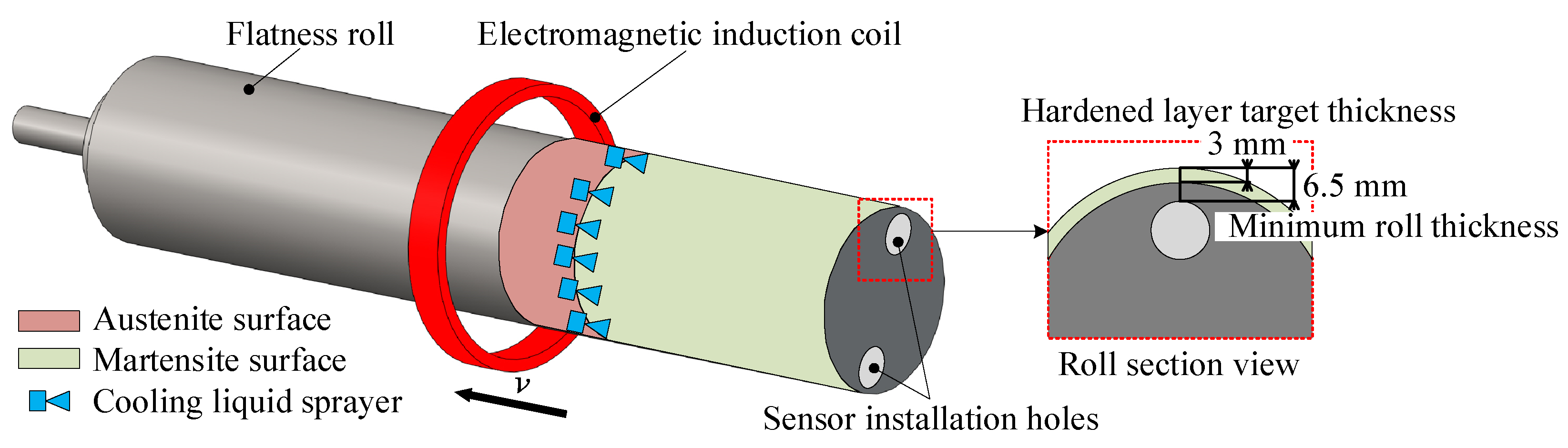
The moving induction quenching process of the flatness roll is shown in
Figure 1. The electrically energized coil surrounds the roll body and moves along the axial direction at a process-set speed
v, heating the roll and causing the matrix pearlitic structure to undergo a diffusion phase transformation to austenite. After a period of heating, the cooling liquid is introduced and the sprayer, which also surrounds the roll body, moves synchronously with the coil. This process causes the transition structure in the surface austenite to undergo a non-diffusion phase transformation to martensite, forming a hardened layer on the roll surface.
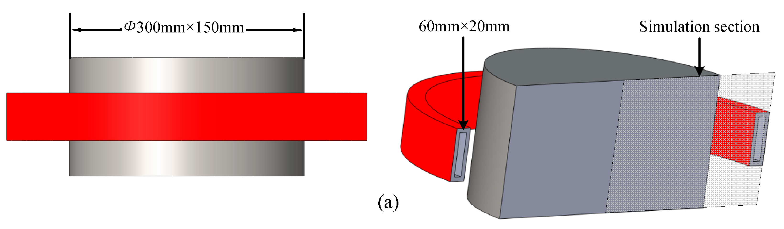
The process described above is simulated using COMSOL Multiphysics 5.5. The 3D schematic diagram of the model, dimensions, observation point locations, and mesh division are shown in
Figure 2. The induction heating 3D structure used for the simulation is shown in
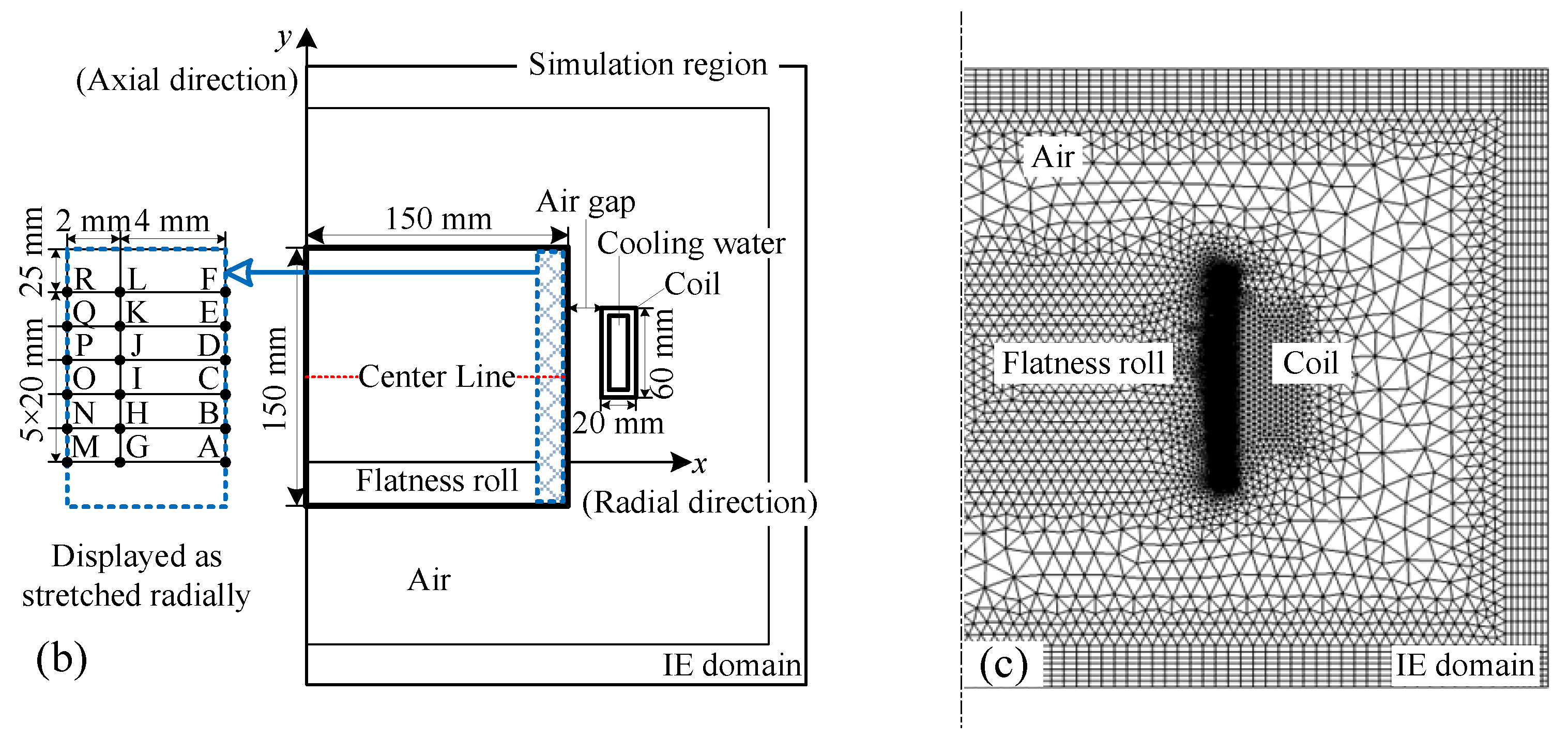
Figure 2a. The roll body specification is Φ 300 mm × 150 mm, and the coil cross-sectional dimensions are 60 mm × 20 mm. The space between the roll body and the coil is filled with air, with a gap of 12 mm between them. The coil cross-section is filled with cooling liquid. Each part of the model is made of the same material and is homogeneous. Due to the axisymmetric nature of the 3D model, it was simplified into a 2D model. A total of 18 observation points were taken along the roll surface and below it, numbered from A to R. The centerline of the model was used as the observation path. The dimensions and observation point locations of the 2D model are shown in
Figure 2b. It was assumed that the internal roll body follows Ampère’s law, and an infinite element domain [
21,
22] (essentially a diffusion-type control equation) is introduced, surrounding the entire simulation space, to model magnetic field dissipation. The boundary of the infinite element domain is set as magnetic insulation so that the high-frequency magnetic field generated by the induction coil only propagates within this region. Due to the skin effect, phase transformation mainly occurs in the surface region during induction heating.
By comparing the results from coarse, baseline, and refined meshes, convergence of multi-physics fields was verified by setting specific convergence criteria for the electromagnetic field, temperature field and stress field, respectively, and ensuring overall error control through coupled iterations. Using the single-variable variation method, the sensitivity of mesh density to stress concentration areas at the coil edges and roller ends was quantified (error reduced to <2%), with results meeting industrial standards. Based on an error estimator, the mesh density in critical regions (e.g., coil and roll edges) was dynamically adjusted to balance accuracy and computational efficiency. Through a local mesh partitioning strategy, the total number of mesh elements was controlled within 30,000. A dual criterion—residual <1 × 10
−5 and temperature gradient variation in critical regions <1%—was adopted to ensure result stability. A fine mesh with a size of 0.2 mm is applied to the surface layer, with a thickness of 10 mm. The infinite element domain uses a mapped mesh with seven layers of elements. The remaining regions use conventional triangular mesh sizes, as shown in
Figure 2c.
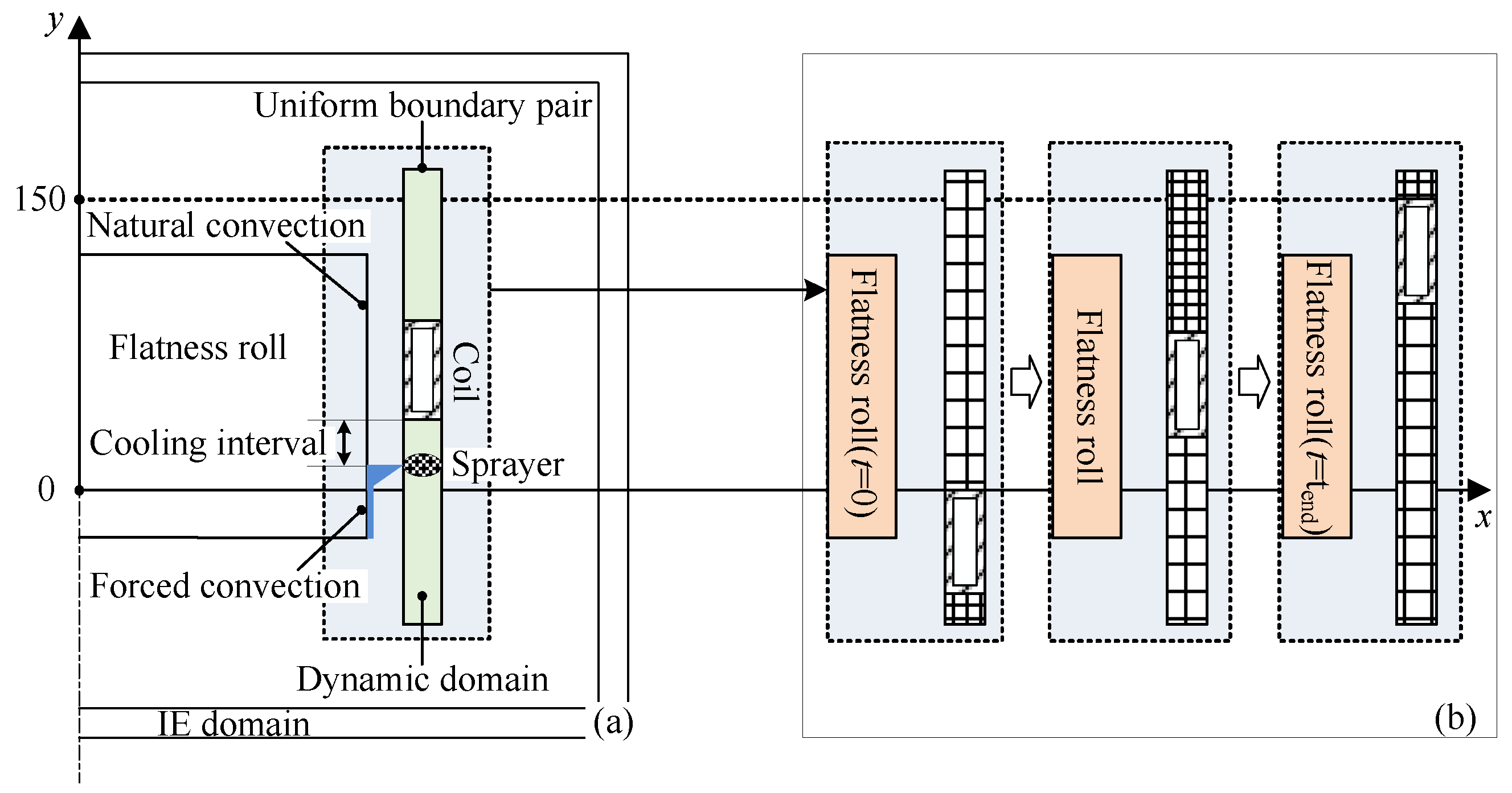
The boundary conditions of the model and the time-varying mesh division within the dynamic domain are shown in
Figure 3. During the moving induction quenching process, as the coil moves upwards, the lower surface area undergoes austenitization and the high-temperature region of the roll body experiences enhanced thermal radiation. After the coil passes the cooling interval, the sprayer begins spraying cooling liquid. The cooling liquid, under the effect of its own weight, causes the region of the roll body below the sprayer to undergo forced convection, while the area above it remains under natural convection with air. In the heating completion phase, the coil stops heating, but the sprayer continues to move and operate. When the sprayer reaches above the roll body, the entire roll surface undergoes forced convection with the cooling liquid.
Figure 3a is a schematic diagram of the model boundary condition changes. As can be seen, the simulation model needs to comprehensively set the boundary condition changes according to the actual situation at each stage [
23,
24].
The dynamic mesh is introduced to simulate the coil mesh movement process [
25,
26], enabling the continuous movement of the coil mesh. A consistent boundary pair is added to the model to divide the dynamic domain (the coil movement range, i.e., the area in which the mesh size changes in the figure) and the static domain (the stationary region outside the dynamic domain). The mesh within the dynamic domain is re-meshed in real time as the coil moves, as shown in
Figure 3b.
The initial overall temperature of the model is set to 20 °C, and a single-turn coil is used with the initial magnetic vector potential, set to 0. The incoming material is set as a 100% uniformly distributed pearlite structure.
5. Optimization of Moving Induction Quenching Process
The Taguchi method was used to optimize the induction quenching process, with the target value for the hardened layer depth set to 3 mm. An orthogonal experiment using a five-factor, four-level table was conducted. The five factors for evaluating the depth and uniformity of the hardened layer were the coil current density (
P1), moving speed (
P2), coil starting position (
P3), spray interval (
P4), and coil position at the end of heating (
P5). Based on the simulation model results, corresponding levels were selected for each factor, and the other levels were adjusted with small disturbances. The four levels of five factors are shown in
Table 3, and the sixteen sets of orthogonal experimental processes are shown in
Table 4.
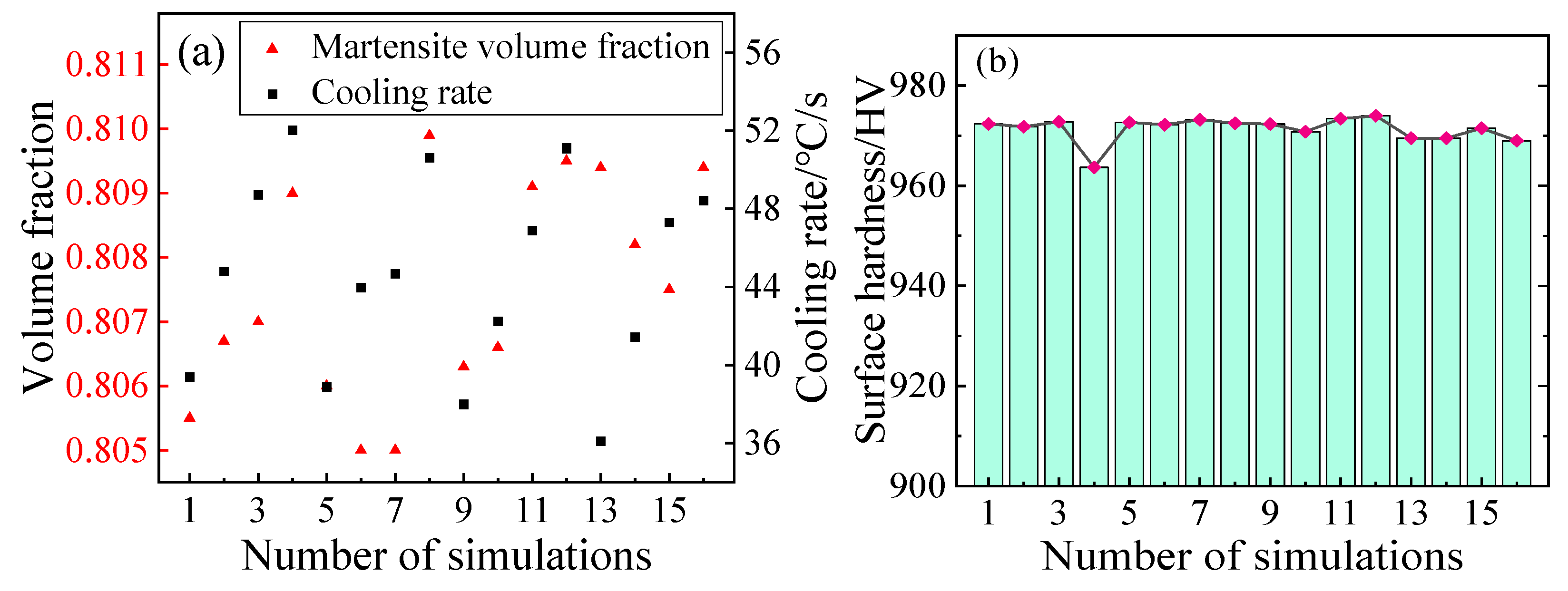
The model was recalculated according to the 16 sets of process parameters in the orthogonal table. The resulting martensite volume fraction at the centerline of the roll body, the cooling rate, and the surface hardness for the 16 sets are shown in
Figure 11. The surface hardness remained largely consistent under different process parameters, although significant differences were noted in the cooling rate and phase proportions at the center. It was therefore concluded that the post-quenching surface hardness primarily depends on the cooling capacity of the cooling liquid.
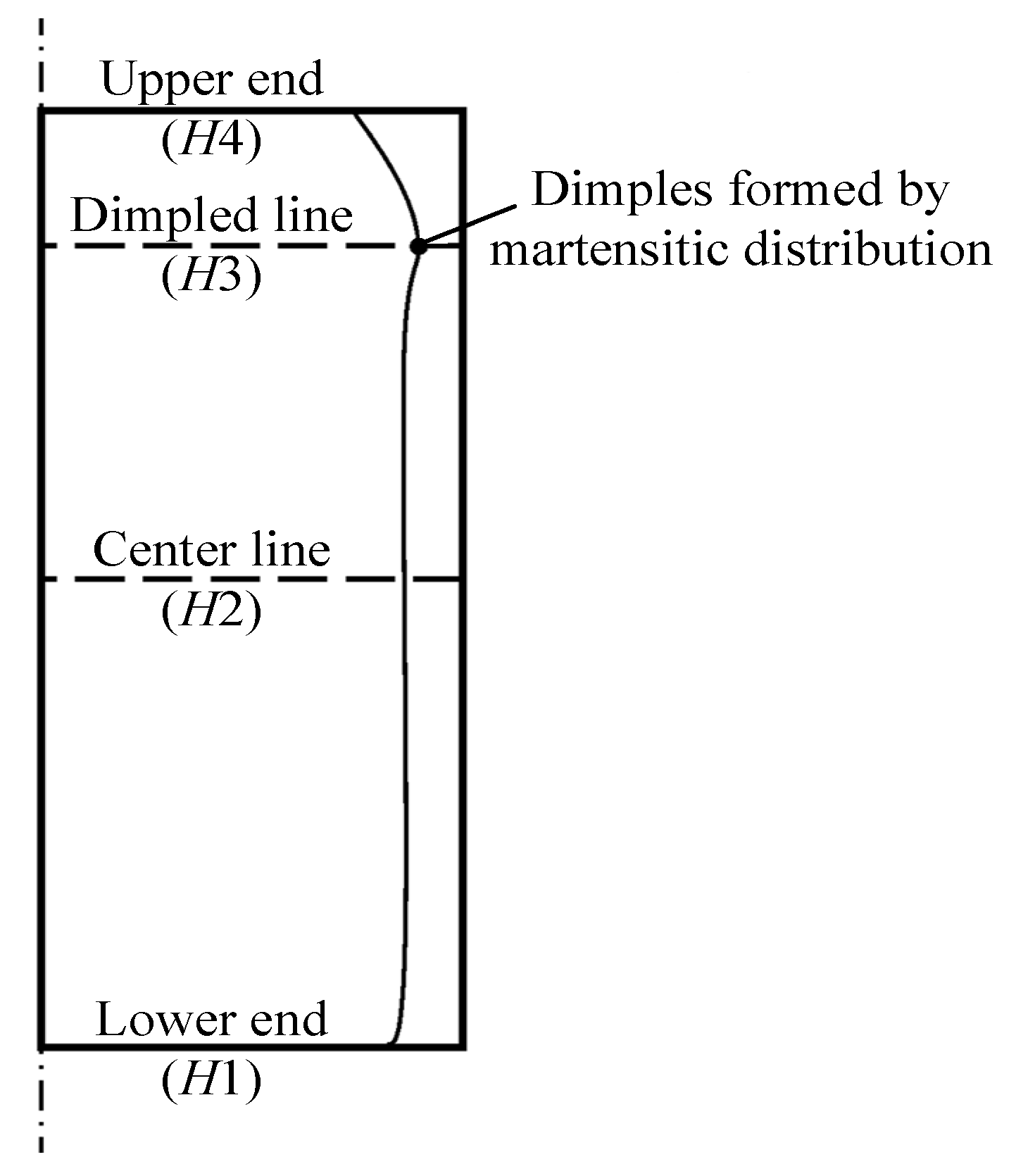
The designed orthogonal experimental table was substituted into the model, and the martensite depth at the lower end line, centerline, dimpled line, and upper end line positions was obtained after calculation, with the values denoted as
H1,
H2,
H3, and
H4, respectively, and with the line positions shown in
Figure 12. The influence weights of each parameter to be optimized on the current evaluation index were calculated, and the results are shown in
Table 5.
It can be seen that the martensite depth at the upper end face H4 was most influenced by P1; H1, H2, and H3 were mainly influenced by the coil moving speed P2, indicating that P2 played a decisive role in the depth of the hardened layer after quenching. Moreover, H1 was also influenced by P5. H2 was almost only affected by P2. H3 was also influenced by P4, P5. H4 was also influenced by P4, P5, and P2, and hardly affected by P3. After repeated simulations and comprehensive consideration, P1 was selected at level 1, P2 at level 1, P3 at level 2, P4 at level 3, and P5 at level 2.
The continuous induction quenching simulation was carried out again with the selected parameters, and the temperature variation at each point on the surface and the martensite depth (
H1~
H4) at each position after optimization are shown in
Figure 13.
It can be seen that compared to the original process, the maximum temperature near the upper and lower ends of the roll body had significantly decreased, effectively preventing material overburning caused by excessively high temperatures. The temperature variation trends at each point show good consistency, which resulted in a more uniform distribution of the hardened layer. Although not completely consistent, the dimpled area had largely been filled. H1~H4 were all close to the target value of 3 mm, effectively reducing the locally high residual stresses and significantly lowering the risk of cracking when the roll surface is subjected to loading.
Author Contributions
Conceptualization, H.Y. and S.L. (Shuang Liao); methodology, H.Y.; software, S.L. (Shan Li); validation, H.Y., S.L. (Shuang Liao) and Z.L.; formal analysis, Z.X.; investigation, S.L. (Shuang Liao); data curation, Z.L.; writing—original draft preparation, H.Y.; writing—review and editing, S.L. (Shuang Liao).; visualization, Z.X. and S.L. (Shan Li); project administration, H.Y.; funding acquisition, H.Y. All authors have read and agreed to the published version of the manuscript.
Funding
This research was funded by National Natural Science Foundation of China, grant number U21A20118 and S&T Program of Hebei, grant number 246Z1601G.
Data Availability Statement
The original contributions presented in this study are included in the article. Further inquiries can be directed to the corresponding author.
Acknowledgments
The studies were carried out on the equipment of the National Engineering Research Center for Equipment and Technology of Cold Rolling Strip of Yanshan University.
Conflicts of Interest
The authors declare no conflict of interest.
References
- Xu, Y.H.; Wang, D.C.; Duan, B.W.; Liu, H.M. Data-driven flatness intelligent representation method of cold rolled strip. J. Iron. Steel Res. Int. 2023, 30, 994–1012. [Google Scholar]
- Zhao, J.W.; Li, J.D.; Yang, Q.; Wang, X.C.; Ding, X.X.; Peng, G.Z.; Shao, J.; Gu, Z.W. A novel paradigm of flatness prediction and optimization for strip tandem cold rolling by cloud-edge collaboration. J. Mater. Process. Technol. 2023, 316, 117947. [Google Scholar] [CrossRef]
- Zhou, G.Y.; Li, H.; He, A.R.; Liu, C.; Sun, W.Q.; Liu, Z.Q.; Han, C. Simulation and control of high-order flatness defect in rolling wide titanium strip with 20-high mill. Int. J. Adv. Manuf. Technol. 2022, 120, 5483–5496. [Google Scholar] [CrossRef]
- Peng, W.; Lei, J.W.; Ding, C.Y.; Yue, C.X.; Ma, G.S.; Sun, J.; Zhang, D.Y. A novel deep ensemble reinforcement learning based control method for strip flatness in cold rolling steel industry. Eng. Appl. Artif. Intell. 2024, 134, 108695. [Google Scholar]
- Zhang, T.Y.; Liao, S.; Gao, J.T.; Hao, W.K.; Liu, H.M. Analysis of Generation Mechanism of Unimodal and Bimodal Waveform Detection Signals of a Whole Roll Flatness Meter. ISIJ Int. 2024, 64, 1783. [Google Scholar]
- Zhang, S.; Liao, S.; Li, S.; Zhang, T.Y.; Yu, H.X.; Liu, H.M. Study on Wear Resistance Evolution of Cold-Rolled Strip Flatness Meter Surface-Strengthened Layer. Metals 2023, 13, 914. [Google Scholar] [CrossRef]
- Zhang, S.; Yu, H.X.; Li, S.; Liao, S.; Zhang, T.Y.; Liu, H.M. Laser Cladding Strengthening Test on the Surface of Flatness Rollers. ISIJ Int. 2023, 63, 120. [Google Scholar]
- Šapek, A.; Kalin, M.; Godec, M.; Donik, Č.; Markoli, B. Effect of feed rate during induction hardening on the hardening depth, microstructure, and wear properties of tool-grade steel work roll. J. Mater. Sci. 2024, 19, 42. [Google Scholar] [CrossRef]
- Liu, L.G.; Yu, H.; Yang, Z.Q.; Zhao, C.M.; Zhai, T.G. Optimization of induction quenching processes for HSS roll based on MMPT model. Metals 2019, 9, 663. [Google Scholar] [CrossRef]
- Lu, S.Q.; Liu, H.C. Effect of Different Microstructures on Surface Residual Stress of Induction-Hardened Bearing Steel. Metals 2024, 14, 201. [Google Scholar] [CrossRef]
- Derouiche, K.; Garois, S.; Champaney, V.; Daoud, M.; Traidi, K.; Chinesta, F. Data-driven modeling for multiphysics parametrized problems-application to induction hardening process. Metals 2021, 11, 738. [Google Scholar] [CrossRef]
- Fang, T.H.; Cai, F. Effects of Surface Softening on the Mechanical Properties of an AISI 316L Stainless Steel under Cyclic Loading. Metals 2021, 11, 1788. [Google Scholar] [CrossRef]
- Jian, S.C.; Wang, J.X.; Xu, D.; Ma, R.; Huang, C.W.; Lei, M.; Liu, D.; Wan, M.P. Gradient microstructure and mechanical properties of Ti-6Al-4V titanium alloy fabricated by high-frequency induction quenching treatment. Mater. Des. 2022, 222, 111031. [Google Scholar]
- Gao, J.W.; Han, R.P.; Zhu, S.P.; Zhao, H.; Correia, J.A.F.O.; Wang, Q.Y. Influence of induction hardening on the damage tolerance of EA4T railway axles. Eng. Fail. Anal. 2023, 143, 106916. [Google Scholar]
- Smalcerz, A.; Barglik, J.; Kuc, D.; Ducki, K.; Wasinski, S. The microstructure and mechanical properties of cylindrical elements from steel 38Mn6 after continuous induction heating. Arch. Metall. Mater. 2016, 61, 1969–1974. [Google Scholar]
- Garstka, T.; Jagiela, K.; Gala, M. Investigations of the hardened layers by means of Barkhausen noise method. Pre. Elektrotechniczn 2010, 86, 41–44. [Google Scholar]
- Choi, J.K.; Park, K.S.; Lee, S.S. Prediction of High-Frequency Induction Hardening Depth of an AISI 1045 Specimen by Finite Element Analysis and Experiments. Int. J. Precis. Eng. Manuf. 2018, 19, 1821–1827. [Google Scholar]
- Slatter, T.; Lewis, R.; Jones, A.H. The influence of induction hardening on the impact wear resistance of compacted graphite iron (CGI). Wear 2011, 270, 302–311. [Google Scholar]
- Nguyen, V.T.; Minh, P.S.; Dang, H.S.; Ho, N. Optimization of arc quenching parameters for enhancing surface hardness and line width in S45C steel using Taguchi method. PLoS ONE 2024, 19, e0314648. [Google Scholar]
- Li, J.J.; Zhang, P.; Hu, J.L.; Zhang, Y.F. Study of the synergistic effect of induction heating parameters on heating efficiency using taguchi method and response surface method. Appl. Sci. 2022, 13, 555. [Google Scholar] [CrossRef]
- Haji, T.K.; Faramarzi, A.; Metje, N.; Chapman, D.; Rahimzadeh, F. Development of an infinite element boundary to model gravity for subsurface civil engineering applications. Int. J. Numer. Anal. Methods Geomech. 2020, 44, 418–431. [Google Scholar]
- Gozalpour, F.; Yavari, M. 2-D Axisymmetric Modeling of Circular PCB Coils and Solenoids in COMSOL Multiphysics. In Proceedings of the 2023 5th Iranian International Conference on Microelectronics (IICM), Tehran, Iran, 25–26 October 2023; pp. 102–106. [Google Scholar]
- Kubota, H.; Tomizawa, A.; Yamamoto, K.; Okada, N.; Hama, T.; Takuda, H. Finite element analysis of three-dimensional hot bending and direct quench process considering phase transformation and temperature distribution by induction heating. ISIJ Int. 2014, 54, 1856–1865. [Google Scholar]
- Areitioaurtena, M.; Segurajauregi, U.; Fisk, M.; Cabello, M.J.; Ukar, E. Numerical and experimental investigation of residual stresses during the induction hardening of 42CrMo4 steel. Eur. J. Mech. A/Solids 2022, 96, 104766. [Google Scholar]
- Yi, Q.Y.; Lan, J.Q.; Ye, J.H.; Zhu, H.C.; Yang, Y.; Wu, Y.Y.; Huang, K.M. A simulation method of coupled model for a microwave heating process with multiple moving elements. Chem. Eng. Sci. 2021, 231, 116339. [Google Scholar] [CrossRef]
- Yuan, X.J.; Ling, H.T.; Chen, J.J.; Feng, Y.; Qiu, T.Y.; Zhao, R.C. A dynamic modelling method for an electro-hydraulic proportional valve combining multi-systems and moving meshes. J. Braz. Soc. Mech. Sci. Eng. 2022, 44, 304. [Google Scholar]
- Iżowski, B.; Wojtyczka, A.; Motyka, M. Numerical Simulation of Low-Pressure Carburizing and Gas Quenching for Pyrowear 53 Steel. Metals 2023, 13, 371. [Google Scholar] [CrossRef]
- Oanh, N.T.H.; Viet, N.H. Precipitation of M23C6 Secondary Carbide Particles in Fe-Cr-Mn-C Alloy during Heat Treatment Process. Metals 2020, 10, 157. [Google Scholar] [CrossRef]
- Tan, Z.; Guo, G.Y. Thermophysical Properties of Engineering Alloys; Metallurgical Industry Press: Beijing, China, 1994. [Google Scholar]
- Maynier, P.H.; Dollet, J.; Bastien, P. Prediction of microstructure via empirical formulas based on CCT diagrams. Metall. Soc. AIME 1978, 1977, 163–178. [Google Scholar]
- Krauss, G. Steels: Heat Treatment and Processing Principles; ASM International: Materials Park, OH, USA, 1990; p. 457. [Google Scholar]
- Zhang, Y.F. Numerical Simulation and Experimental Study on Carburizing-Quenching Process of 18CrNiMo7-6 alloy Steel. Master’s Thesis, Zhengzhou University, Zhengzhou City, China, 2019. [Google Scholar]
Figure 1.
Process of moving induction quenching for flatness rolls.
Figure 2.
(a) The 3D schematic diagram of the model; (b) Dimensions and location of observation points; (c) Mesh division situation.
Figure 3.
(a) Model boundary conditions; (b) Time-varying mesh division within the dynamic domain.
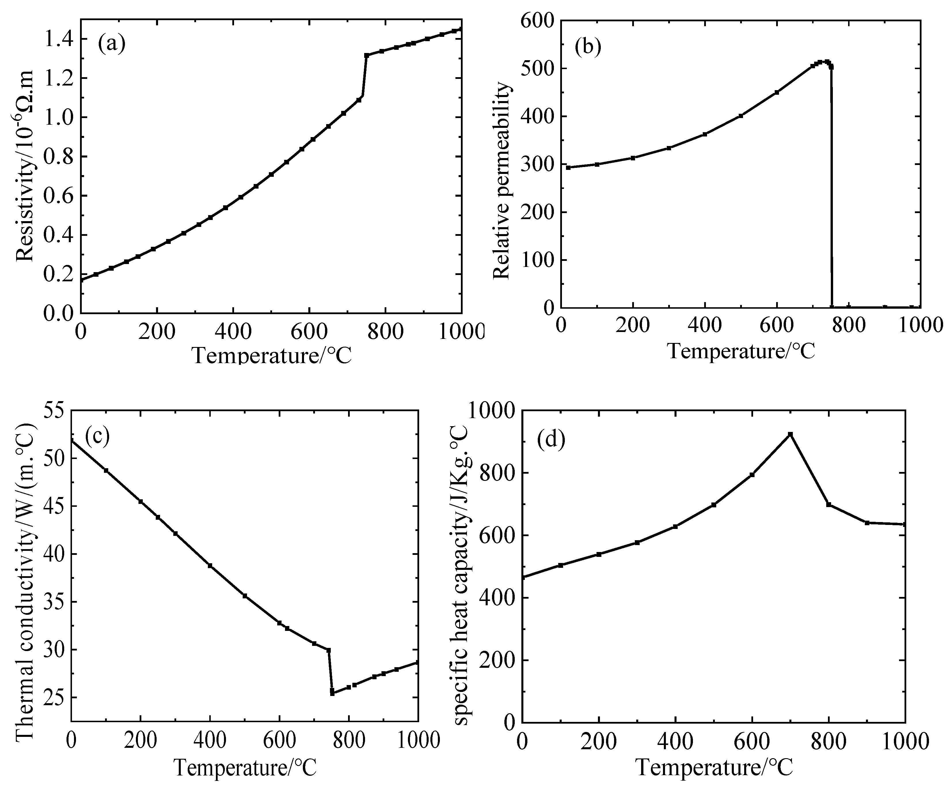
Figure 4.
Temperature-dependent curves of (a) resistivity; (b) relative magnetic permeability; (c) thermal conductivity; and (d) specific heat of MC3.
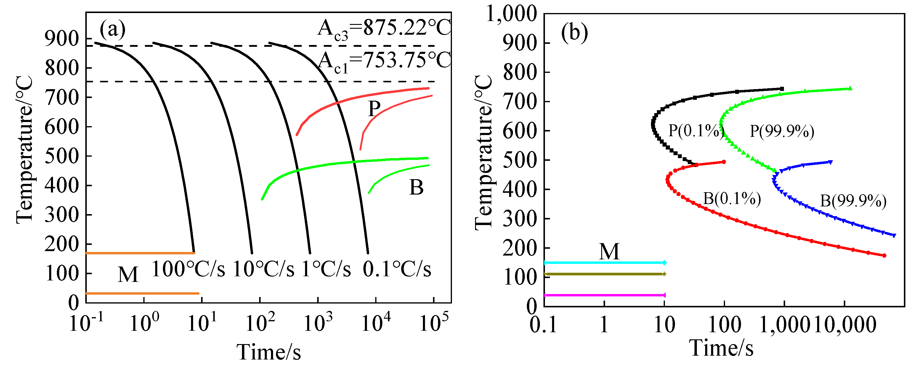
Figure 5.
(a) CCT curve; (b) TTT curve of MC3.
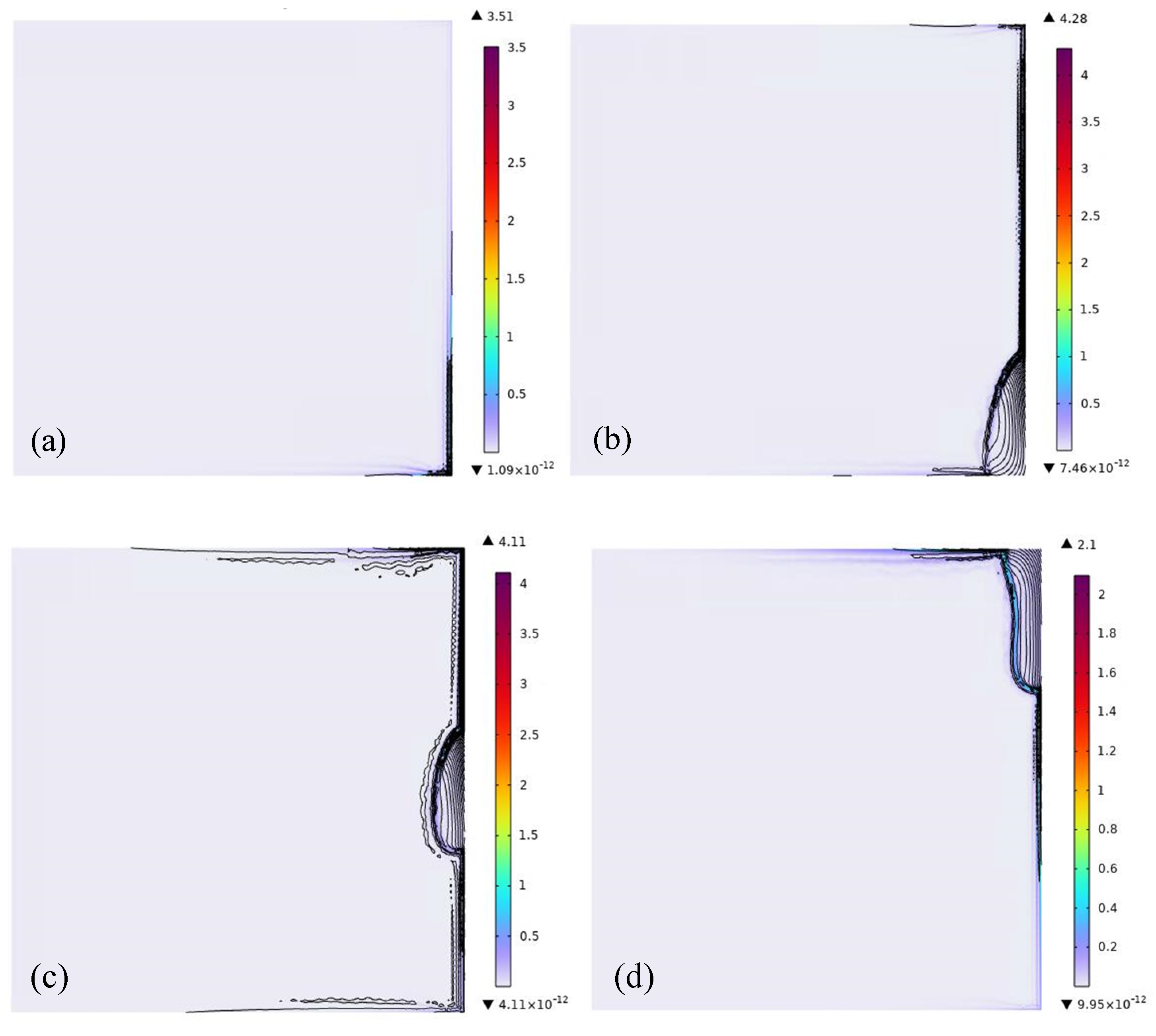
Figure 6.
Distribution of the electromagnetic field at the roll body cross-section: (a) 0 s; (b) 50 s; (c) 100 s; and (d) 150 s after processing begins.
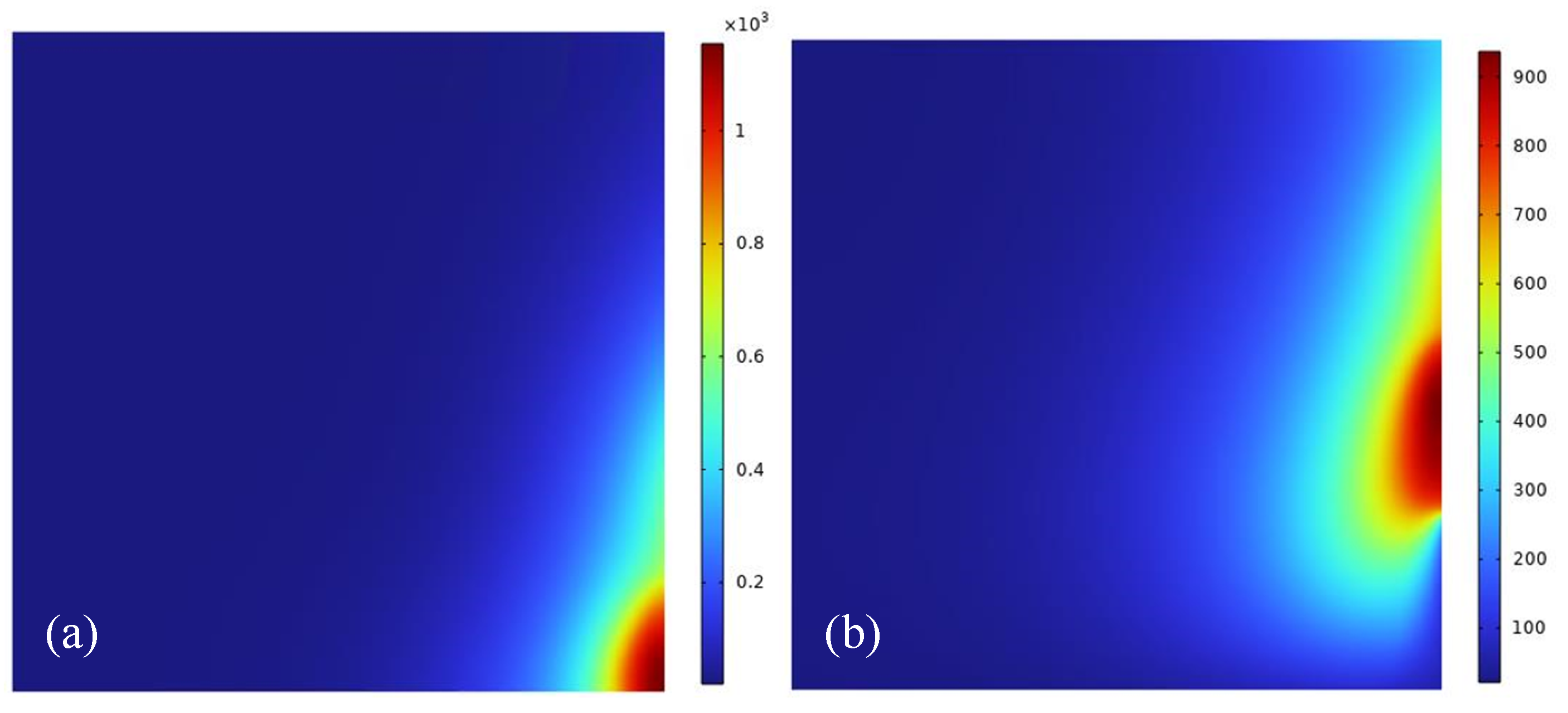
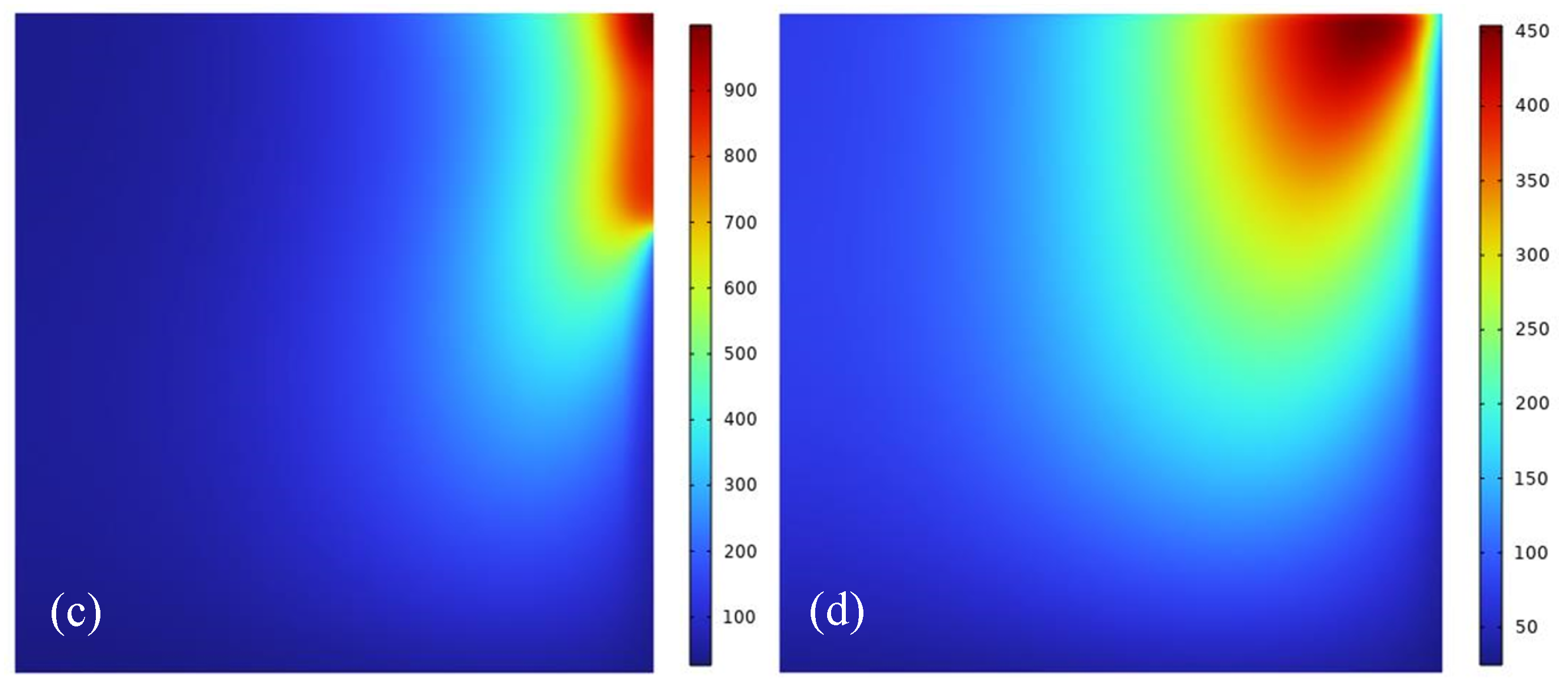
Figure 7.
Distribution of the temperature field at the roll body cross-section: (a) 30 s; (b) 90 s; (c) 150 s; and (d) 200 s after processing begins.
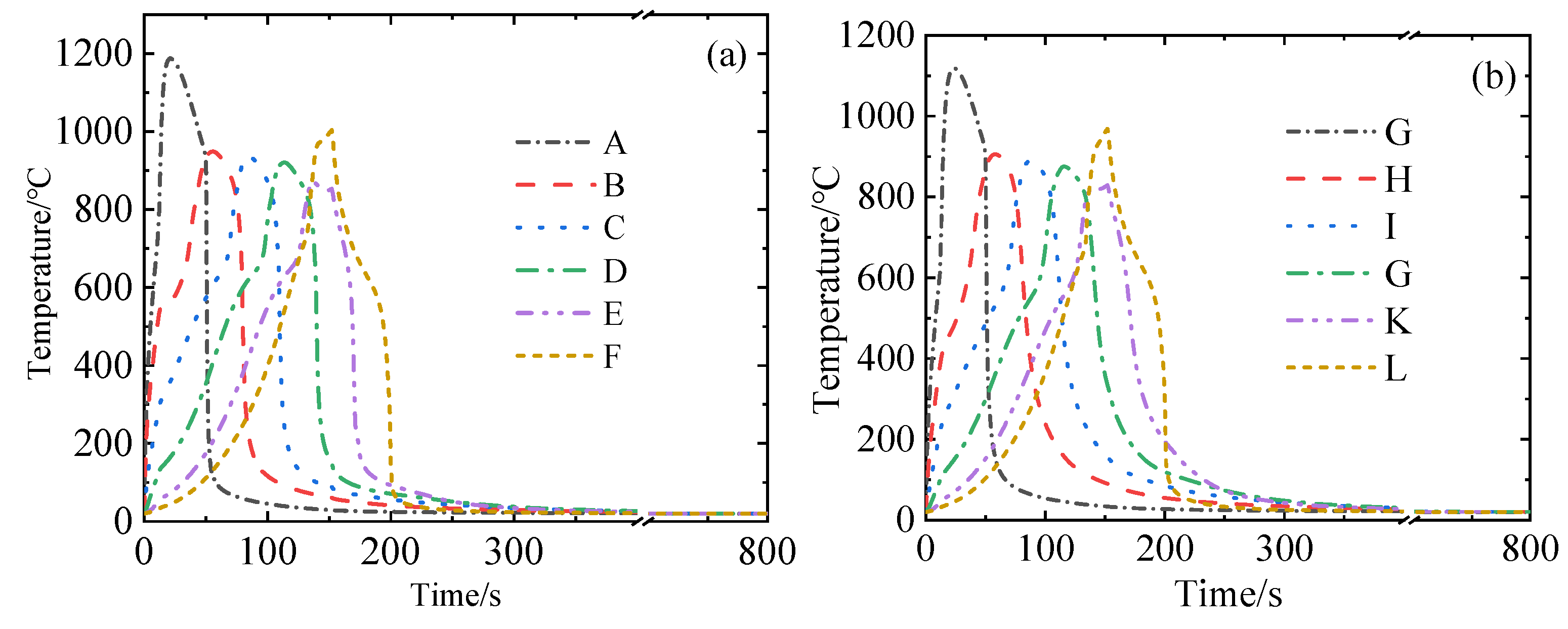
Figure 8.
Time-varying temperature curves at two sets of observation points: (a) surface; (b) internal.
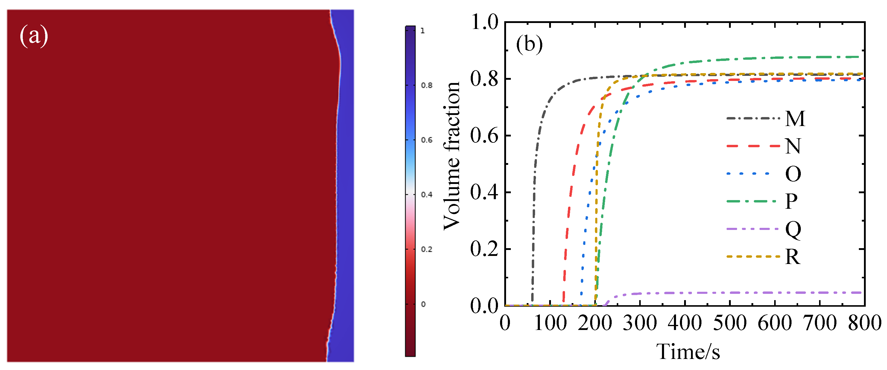
Figure 9.
(a) Martensite distribution within the cross-section; (b) Time-varying martensite volume fraction at the internal observation points after quenching.
Figure 10.
Volume fraction of austenite at centerline of the roll cross-section after quenching.
Figure 11.
(a) Martensite volume fraction and cooling rate at the centerline of the roll body; (b) Surface hardness for the 16 sets of process parameters.
Figure 12.
Line positions for the lower end line, centerline, dimpled line, and upper end line.
Figure 13.
(a) Temperature variation at points A~F on the surface after optimization; (b) Martensite depth (H1~H4) at each position.
Figure 14.
(a) Cooling curves at different thicknesses along the centerline of the roll body; (b) Temperature and hardness distribution along the centerline after quenching.
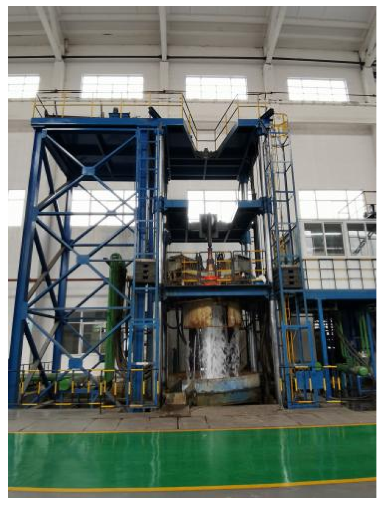
Figure 15.
Vertical high-frequency induction quenching equipment for rolls.
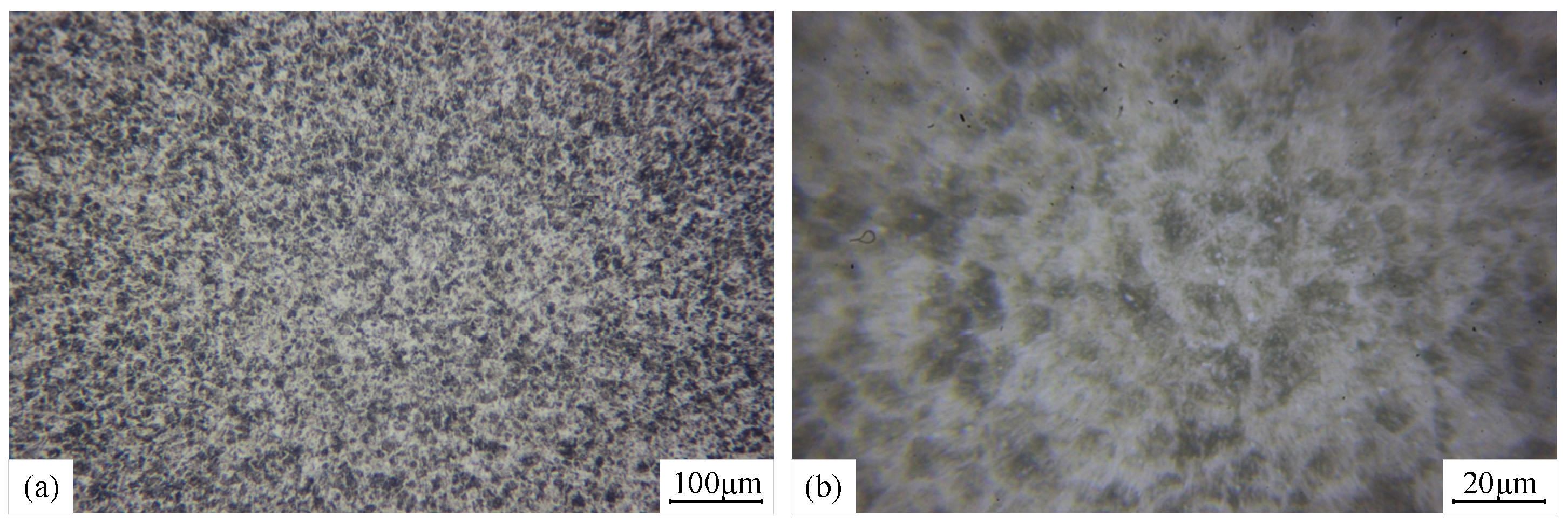
Figure 16.
Post-quenching microstructure: (a) 100× magnification; (b) 500× magnification.
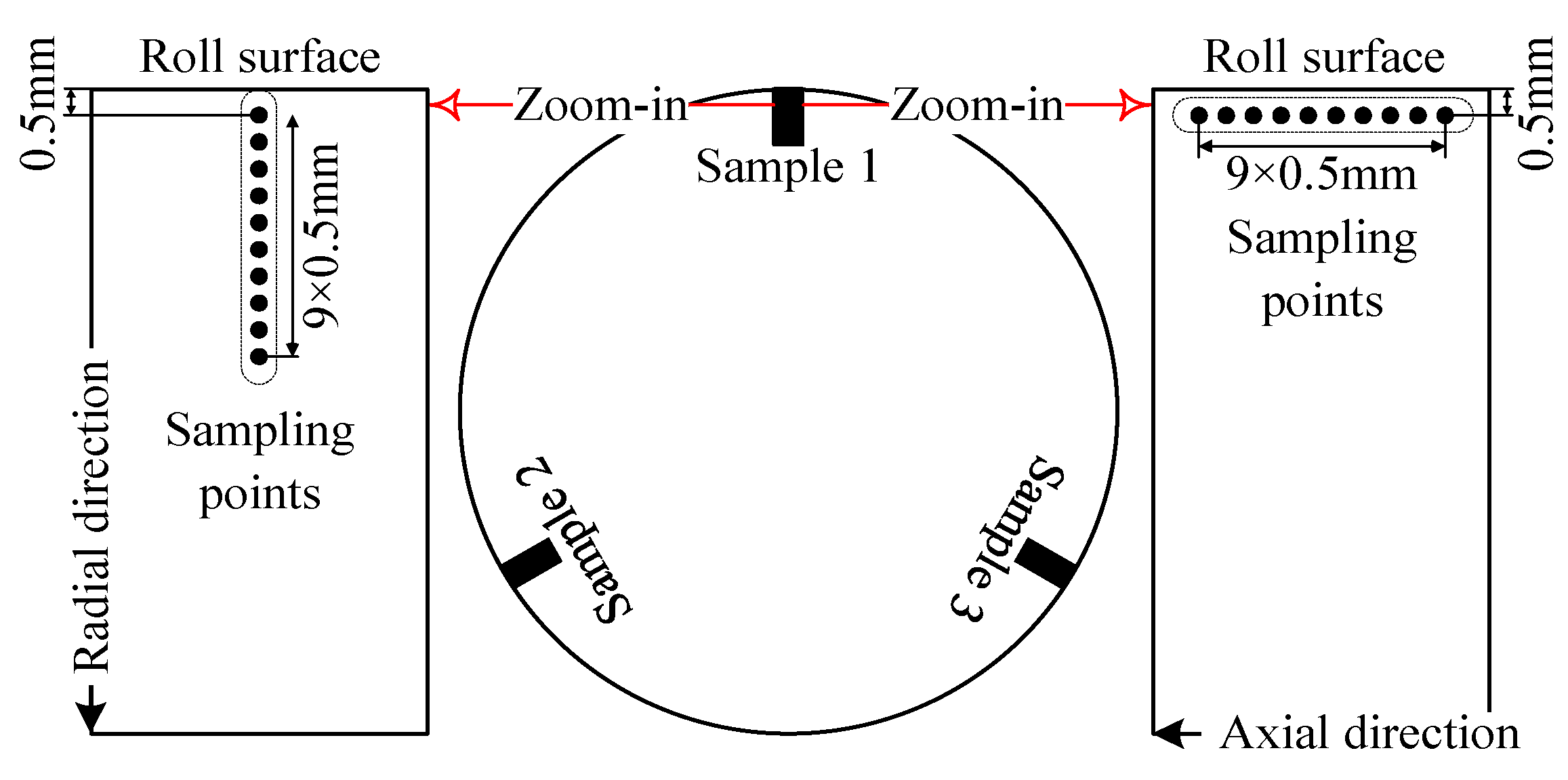
Figure 17.
Schematic diagram of the sampling locations along the axial and radial directions of the roll body.
Table 1.
Main chemical composition of MC3 (wt.%).
| Element | C | Mn | Cr | Mo | V | Si | S | P | Ni |
|---|
| Content | 0.87 | 0.58 | 2.92 | 0.3 | 0.12 | 0.45 | 0.009 | 0.014 | 0.7 |
Table 2.
Selected simulation parameters.
| Current Frequency (Hz) | Current Density (A/m2) | Air Gap (mm) | Moving Speed (mm/s) | Cooling Interval (s) | Initial Coil Position (mm) | Heating Time (s) | Total Time (s) |
|---|
| 7000 | 7 × 10⁶ | 12 | 1 | 50 | y = 0 | 150 | 800 |
Table 3.
Four levels of five factors of moving induction quenching processes.
| Experimental Factors | P1 (A/m2) | P2 (mm/s) | P3 (mm) | P4 (s) | P5 (mm) |
|---|
| Level 1 | 6.1 × 10⁶ | 0.8 | −25 | 36 | 130 |
| Level 2 | 6.15 × 10⁶ | 0.9 | −27.5 | 38 | 131 |
| Level 3 | 6.26 | 1 | −30 | 40 | 132 |
| Level 4 | 6.25 × 10⁶ | 1.1 | −32.5 | 42 | 133 |
Table 4.
Sixteen sets of orthogonal experimental processes.
| Number of Experiments | P1 (A/m2) | P2 (mm/s) | P3 (mm) | P4 (s) | P5 (mm) |
|---|
| 1 | 6100 | 0.8 | −25 | 36 | 130 |
| 2 | 6100 | 0.9 | −27.5 | 38 | 131 |
| 3 | 6100 | 1 | −30 | 40 | 132 |
| 4 | 6100 | 1.1 | −32.5 | 42 | 133 |
| 5 | 6150 | 0.8 | −27.5 | 40 | 133 |
| 6 | 6150 | 0.9 | −25 | 42 | 132 |
| 7 | 6150 | 1 | −32.5 | 36 | 131 |
| 8 | 6150 | 1.1 | −30 | 38 | 130 |
| 9 | 6200 | 0.8 | −30 | 42 | 131 |
| 10 | 6200 | 0.9 | −25 | 40 | 130 |
| 11 | 6200 | 1 | −32.5 | 38 | 133 |
| 12 | 6200 | 1.1 | −27.5 | 36 | 132 |
| 13 | 6250 | 0.8 | −32.5 | 38 | 132 |
| 14 | 6250 | 0.9 | −30 | 36 | 133 |
| 15 | 6250 | 1 | −27.5 | 42 | 130 |
| 16 | 6250 | 1.1 | −25 | 40 | 131 |
Table 5.
Influence weights of each optimization parameter.
| | H1 | H2 | H3 | H4 |
|---|
| | SSD | Weight (%) | SSD | Weight (%) | SSD | Weight (%) | SSD | Weight (%) |
|---|
| P1 | 1.5734 | 7.94 | 0.0721 | 2.8 | 0.6409 | 6.32 | 0.4826 | 39.27 |
| P2 | 12.5 | 63.11 | 2.4262 | 94.64 | 10.1048 | 67.91 | 0.2152 | 17.89 |
| P3 | 1.5727 | 7.94 | 0.0109 | 0.4 | 0.9267 | 6.23 | 0.0067 | 0.54 |
| P4 | 1.5727 | 7.94 | 0.0316 | 1.23 | 1.95 | 13.11 | 0.2936 | 23.86 |
| P5 | 2.5877 | 13.07 | 0.0227 | 0.93 | 1.2564 | 12.43 | 0.5258 | 18.44 |
| Total | 19.807 | 1 | 2.5635 | 1 | 14.879 | 1 | 1.231 | 1 |
Table 6.
Radial hardness distribution.
| Position | 1 | 2 | 3 | 4 | 5 | 6 | 7 | 8 | 9 | 10 |
|---|
| 890.3 | 885.2 | 881.6 | 876.7 | 872.6 | 741.5 | 460.3 | 346.3 | 344.7 | 342.3 |
| 957.2 | 951.8 | 950.5 | 947.5 | 945.0 | 783.3 | 456.1 | 343.5 | 343.6 | 343.5 |
| Error | −7.5 | −7.6 | −7.8 | −8.1 | −8.3 | −5.6 | −2.9 | 0.08 | 0.03 | −0.04 |
Table 7.
Axial hardness distribution.
| Position | 1 | 2 | 3 | 4 | 5 | 6 | 7 | 8 | 9 | 10 | Average |
|---|
| 894.4 | 886.4 | 890.2 | 892.1 | 889.0 | 898.7 | 893.4 | 900.2 | 897.6 | 898.2 | 893.7 |
| 957.4 | 957.2 | 958.1 | 957.1 | 957.6 | 957.4 | 958.2 | 958.8 | 957.3 | 957.4 | 957.3 |
| Error | 7.0 | 8.0 | 7.6 | 7.3 | 7.6 | 6.6 | 7.3 | 6.4 | 6.3 | 6.6 | 7.1 |
| Disclaimer/Publisher’s Note: The statements, opinions and data contained in all publications are solely those of the individual author(s) and contributor(s) and not of MDPI and/or the editor(s). MDPI and/or the editor(s) disclaim responsibility for any injury to people or property resulting from any ideas, methods, instructions or products referred to in the content. |
© 2025 by the authors. Licensee MDPI, Basel, Switzerland. This article is an open access article distributed under the terms and conditions of the Creative Commons Attribution (CC BY) license (https://creativecommons.org/licenses/by/4.0/).


