A Statistical-Based Model of Roll Force During Commercial Hot Rolling of Steel

Abstract

This research introduces a new model to predict the roll force during hot rolling of steel, based on a statistical analysis of approximately 38,980 sets of measurements in a commercial mill with five finishing stands. The study includes ten different steel grades and features models of both single grades and the entire dataset. Three models are developed and compared: a temperature-dependent strain rate model (M1), a strain rate model (M2), and a simplified strain rate model (M3). The decrease in temperature with roll stand has a strong cross-correlation with compensating decreases in strain and contact length by roll stand, such that both the temperature and strain terms are statistically insignificant. The final model (M3)—$F\left[\mathrm{N}\right]=113.1·\dot{ϵ}{\left[{\mathrm{s}}^{-1}\right]}^{0.3141}·w\left[\mathrm{mm}\right]·\ell \left[\mathrm{mm}\right]$—relates force (F) to strain rate ($\dot{ϵ}$), width (w), and contact length (ℓ) and achieves an $R^2$ fit of 0.946 over all 10 steel grades. Although the single-grade models show slightly higher accuracy, the final model retains robust predictive capability with only two fitting parameters. This model enables fast and easy estimation of roll force for commercial hot rolling of low-carbon, medium-carbon, and high-strength–low-alloy steels.

1. Introduction

Hot rolling plays a vital role in steel production, where accurate prediction of roll forces is crucial for product quality, operational efficiency and safety [1,2]. Although numerous types of models have been developed to predict roll forces, their performance across various steel grades and rolling conditions in industrial-scale rolling conditions still warrants more research [3,4].

Predicting roll forces during hot rolling processes is important because inaccurate predictions can lead to serious quality defects, catastrophic operational failures, such as cobbles, and significant safety hazards. When roll forces do not match expected gauge reductions, steel can accumulate between roll stands and fly off the roller conveyor, damaging equipment, and endangering personnel [1]. Furthermore, roll force directly affects roll life, as forces proportional to applied pressure cause progressive roll wear and profile degradation [2]. Roll-wear modeling is particularly significant for operational maintenance scheduling, cost management and associated surface defects on the rolled product, and depends on accurate modeling of roll force [5].

Roll force prediction is difficult because the phenomena which control the steel strength are extremely complex, and include microstructural phenomena at a scale smaller than the grain size up to phenomena at the macroscale of the rolling stands. Traditional approaches to predict roll force often rely on simplified analytical models to convey the results of laboratory measurements. These models require inputs not readily available in commercial settings [3] or involve empirical relationships that do not fully capture the dynamics of industrial-scale operations [4] and microstructural hardening mechanisms. The substantial differences between laboratory conditions and commercial processes with multiple sequential stands create significant challenges [6]. Specifically, the former environment exhibits smaller roll diameters, lower strain rates, single-stand configurations, and often different sample geometries and loading conditions. While recent advancements in data collection have enabled more sophisticated modeling approaches [7], there remains a critical need for simple, accurate, and implementable fundamental models suitable for real-time applications ranging from simple estimates to calculations in commercial hot rolling operations.

This research aims to develop a simple, yet accurate, regression model for predicting roll forces in commercial hot rolling operations across diverse steel grades using an extensive data set from a commercial hot rolling mill. This data set includes measurements across five finishing stands and 10 steel grades, including low carbon, medium carbon, and high-strength-low-alloy (HSLA) steels. This work is an extension of previous (Greivel et al. [8]) and seeks an equation that captures essential physics with as few estimate parameters as possible while maintaining reasonable predictive power. The objective is to provide readers with an easily implementable model that balances accuracy with practical utility.

2. Previous Models

Roll force models have been developed in previous work through several different methodologies, including fundamental equations based on laboratory experiments, finite element analysis, and data-driven statistical techniques. Each approach offers distinct advantages and limitations for predicting forces during hot rolling processes in steel manufacturing. In this section, these modeling approaches are examined to establish the foundation for the new statistical-based model.

2.1. Models of Laboratory-Scale Experiments

Foundational models for roll force prediction have been developed through controlled laboratory experiments, including: hot compression tests [9,10], torsion tests for studying high-strain deformation [11], and small-scale rolling mills [12]. The latter lab mills typically have roll diameters of 100–300 mm, significantly smaller than the 700–1000 mm rolls found in commercial operations.

The pioneering laboratory studies by Jonas et al. [11] established relationships between microstructure evolution and deformation behavior with particular focus on static and dynamic recrystallization of austenite in steels. Based on hot torsion tests at temperatures of 900–1200 °C and strain rates of 0.1–10 s⁻¹, they developed the constitutive equation:

$$\dot{ϵ}=Asinh{\left(\alpha \sigma \right)}^{n}exp\left({\displaystyle \frac{-Q}{RT}}\right)$$

(1)

where $\dot{ϵ}$ is the strain rate [s⁻¹], A is a material constant [s⁻¹], $\alpha$ is the stress multiplier [MPa⁻¹], $\sigma$ is the flow stress [MPa], n is the stress exponent [-], Q is the activation energy for deformation [J/mol], R is the universal gas constant (8.314 J/mol·K), and T is the absolute temperature [K]. For plain carbon steels, they determined activation energies ranging from 300 to 450 kJ/mol, with stress exponents between 3 and 5, and stress multipliers of 0.012–0.015 MPa⁻¹. While these parameters became industry standards, it is important to note that their experimental strain rates were 10 to 100 times lower than those encountered in commercial rolling, where rates can reach 100–1000 s⁻¹.

Building on this foundation, Sellars and McTegart [9] focused on understanding the microstructural evolution during deformation. Using plane strain compression tests in cam plastometers, they explored a wider range of strain rates (0.01–100 s⁻¹) at temperatures of 850–1150 °C, and quantified dynamic recrystallization kinetics with the Avrami equation:

$$X_{DRX}=1-exp\left[-0.693{\left({\displaystyle \frac{t}{t_{0.5}}}\right)}^n\right]$$

(2)

where $X_{DRX}$ is the fraction recrystallized [-], t is the time [s], $t_{0.5}$ is the time for 50% recrystallization [s], and n is the Avrami exponent [-]. They further predicted time for 50% recrystallization:

$$t_{0.5}=A{\dot{ϵ}}^{-p}{ϵ}^{-q}exp\left({\displaystyle \frac{Q_{rx}}{RT}}\right)$$

(3)

where A, p, and q are material constants, $ϵ$ is the strain [mm/mm], and $Q_{rx}$ is the activation energy for recrystallization [J/mol]. For low carbon steels, they found $Q_{rx}$ values between 230 and 270 kJ/mol. However, these interrupted tests cannot replicate the continuous deformation that occurs in multi-stand rolling for which inter-pass times are mere seconds (typically 0.5–2 s), barely allowing partial recrystallization between stands.

Choi et al. [12] investigated deformation path effects using a laboratory rolling mill with 225 mm diameter rolls. They compared plate rolling, which experiences monotonic compressive loading, with bar rolling, where cross-compressive loading due to 90-degree rotation between passes causes finer ferrite grain size and higher yield strength. This difference in properties caused by the different strain paths explains why laboratory studies using different loading conditions, such as compression tests, over-predict recrystallization kinetics compared to industrial rolling [13].

More recently, Ghosh et al. [10] designed compression tests using tantalum foils to lessen friction effects (barreling coefficient < 0.6). Based on Gleeble thermo-mechanical compression tests on Ti+Nb stabilized interstitial free (IF) steel at (650–1100 °C) and low strain rates (0.001–10 s⁻¹), separate constitutive equations for ferrite and austenite were developed [10]:

$$\sigma =({\sigma }_0+K{ϵ}^n){\dot{ϵ}}^{m}exp\left({\displaystyle \frac{Q}{RT}}\right)$$

(4)

where ${\sigma }_0$ is the yield stress [MPa], K is the strength coefficient [MPa], m is the strain rate sensitivity exponent [-], and other terms are as previously defined. This approach yielded $R^2$ values of 0.982 in curve fits for the $\gamma$-phase and 0.936 for the $\alpha$-phase, with an activation energy of 414.6 kJ/mol.

Laboratory rolling mills apply loading conditions closer to those found in the real commercial process, although at reduced scale. Brown and DeArdo [14] used a mill with 200 mm diameter rolls to investigate microstructure evolution in high-strength–low-alloy (HSLA) steels. The measured forces (0.5–2 MN) were an order of magnitude smaller than commercial operations (10–40 MN), but their work revealed crucial insights about retained strain between passes. They developed a model incorporating retained strain between rolling passes to quantify incomplete recrystallization:

$${ϵ}_{ret}={ϵ}_{applied}[1-X_{rx}]$$

(5)

where ${ϵ}_{ret}$ is the retained strain [mm/mm] and ${ϵ}_{applied}$ is the applied strain in the previous pass [mm/mm]. The significance of retained strain lies in its direct impact on flow stress predictions in subsequent passes. When recrystallization is incomplete, the material enters the next stand in a partially work-hardened state, requiring higher forces than predicted by models assuming full softening. They showed that incorporating retained strain into flow stress calculations improved force predictions by 10–15% in multi-pass operations, particularly for microalloyed steels where recrystallization is deliberately suppressed to achieve grain refinement.

Dynamic interactions between stands require consideration of load distribution, as investigated by Jia et al. [15], who developed a multi-objective optimization model for hot strip mills that accounts for rolling force margin balance, roll wear ratio, and strip shape control. Their work demonstrates that coordinated load distribution across stands directly influences product quality, making such considerations particularly relevant to the present work with a five-stand finishing mill, where roll forces must be balanced to maintain product quality while maximizing equipment longevity.

The persistent challenge with all laboratory models is that, when applied to commercial rolling processes, they consistently underpredict flow stress by 20–40%. This systematic error arises from several sources: extrapolation of constitutive equations beyond their calibrated strain rate ranges leading to underprediction of strain rate hardening effects at the 100–1000 s⁻¹ rates typical of commercial mills, the absence of realistic thermal gradients in laboratory tests, and the lack of roll flattening effects that become significant at the high contact pressures encountered in commercial rolling. Additionally, laboratory tests cannot replicate the accumulated strain history from multiple stands. These limitations mean that laboratory models, while invaluable for understanding fundamental mechanisms, require substantial empirical corrections when applied to industrial practice.

2.2. Finite Element Analysis Models

In order to gain a deeper insight into the complex phenomena of hot rolling, researchers have implemented comprehensive computational models that address the intertwined thermal-mechanical equations. These models account for spatial variations in temperature, stress, strain, and displacement fields, along with the impacts of microstructural changes. Notably, finite-element models are adept at representing the helical shape of the coil as it progresses through the roll contact area. Within these models, temperature fields are important due to their significant influence on the microstructure and flow stress. The governing heat equation includes the time-dependent effects of conduction, deformation, and friction heating, expressed as:

$$\rho C_p{\displaystyle \frac{\partial T}{\partial t}}=\nabla ·(k\nabla T)+{\dot{q}}_{plastic}+{\dot{q}}_{friction}$$

(6)

where $\rho$ is the material density [kg/m³], $C_p$ is the specific heat capacity [J/kg·K], T is temperature [K], t is time [s], k is thermal conductivity [W/m·K], ${\dot{q}}_{plastic}$ is the heat generation rate from plastic deformation [W/m³], and ${\dot{q}}_{friction}$ is the heat generation rate from friction [W/m³]. Heat losses from radiation, convection, and conduction to the rolls are incorporated via the boundary conditions. This equation should be solved simultaneously with the much more complex momentum, constitutive, and compatibility equations to simulate the mechanical behavior governing deformation, creating a computationally intensive problem.

Early finite element analysis (FEA) work by Jin et al. [16] demonstrated both the promise and limitations of computational modeling. They developed a 2D plane-strain model for roughing-stand rolling of plain carbon steel, implementing an elastic-viscoplastic constitutive relationship:

$$\sigma =K\left(T\right){ϵ}^n{\dot{ϵ}}^m$$

(7)

where $K\left(T\right)$ is the temperature-dependent strength coefficient [MPa], and n and m are the strain hardening and strain rate sensitivity exponents, respectively. When validated against five industrial rolling cases, their predictions matched within 8% of measured forces, ranging from 15 to 25 MN. Their analysis revealed that about 90% of deformation heat conducts into the rolls, surface temperatures plummet by 150–200 °C during the brief contact time, and neglecting these temperature gradients leads to force underpredictions of 15–20%.

Considering the importance of heat transfer during hot rolling, Devadas et al. [17] quantified heat transfer coefficients based on fitting measured temperatures:

$$h=20+1.5{\displaystyle \frac{P}{{\sigma }_y}}$$

(8)

where h is the heat transfer coefficient [kW/m²·K], P is the contact pressure [MPa], and ${\sigma }_y$ is the material yield stress [MPa]. This equation reveals dramatic changes in heat transfer along the contact length, increasing five-fold from 25 kW/m²·K at entry (and exit) to 120 kW/m²·K at the neutral point. This variation may help to explain why models assuming constant heat transfer coefficients consistently underpredict temperature drops and consequently underestimate roll forces by 10–15%.

Kumar et al. [18] conducted high-resolution finite-element simulations using DEFORM-3D with the Hansel–Spittel constitutive model:

$$\sigma =A{ϵ}^{n_1}{e}^{n_2/T}{\dot{ϵ}}^{n_3}{T}^{n_4}$$

(9)

where A is a material constant [MPa], and $n_1$, $n_2$, $n_3$, and $n_4$ are model parameters specific to each steel grade. For microalloyed steels, they found strain rate exponent values ($n_3$) between 0.13 and 0.22. Their extensive mesh sensitivity studies revealed that at least 50,000 elements are needed to achieve force predictions within 5%. Their model agreed with industrial force measurements within 6.3%, but each simulation required 4–8 h of computation time per rolling pass.

The dynamic nature of rolling, overlooked in steady-state analyses, was investigated by Bagheripoor and Bisadi [19]. Implementing a thermoviscoplastic model with Johnson-Cook flow stress relationships, they uncovered force fluctuations of ±5–8% occurring at frequencies of 10–15 Hz. These variations, caused by roll eccentricity and bearing clearances, translate directly into thickness variations of ±30–50 µm—accounting for approximately 40% of the gauge variation observed in commercial mills.

Clearly, FEA modeling is useful to identify, quantify, and understand the phenomena which govern hot rolling, including accurate force predictions within 5–10% of measurements. However, to achieve such accurate results requires adequate spatial resolution, which results in computation times of 4–24 h per rolling pass, and substantial effort to develop and calibrate the models. Thus, there remains a need for simple, easy-to-use, fast models which capture the essential physics and can make reasonable force predictions.

2.3. Statistical Modeling and Machine Learning Approaches

Statistical methods and machine learning models offer distinct advantages in roll force prediction compared to models based on lab experiments or finite element method models. These empirical models take advantage of large commercial data sets to establish relationships between process variables and roll forces using measurements of real industrial-scale operational data while requiring few computational resources and short development time.

2.3.1. Regression-Based Models

Poliak et al. [20] examined 50,000 plate rolling measurements, determining that 80% of the uncertainty in predicting roll force was due to model shortcomings and process variations, rather than errors in measurement. This encourages the pursuit of improved modeling techniques. The development of linear regression models for roll force by Santos et al. [21] utilized 5000 commercial data points:

$$lnF={\beta }_0+{\beta }_{1}ln\left(\dot{ϵ}\right)+{\beta }_2\left({\displaystyle \frac{1}{T}}\right)+{\beta }_{3}ln\left(ϵ\right)+{\beta }_{4}ln\left(w\right)+{\beta }_{5}ln(\ell )$$

(10)

where F denotes force in Newtons [N], w represents width in millimeters [mm], ℓ indicates contact length in millimeters [mm], and ${\beta }_i$ are regression coefficients. Yet, major multicollinearity involving temperature, strain, and stand position (correlation coefficients exceeding 0.85) led to non-viable outcomes. These included negative activation energies, suggesting an increase in force with rising temperature, which contradicts the expected material softening. Additionally, width exponents showed values from 0.7 to 1.3 instead of the theoretical value of 1.0. Employing ridge regression brought improved fit ($R^2$ = 0.92), although it compromised physical interpretation. The new width exponent of 0.85 failed to accurately capture the true physical influence.

Li et al. [22] addressed multicollinearity differently when predicting the friction coefficient:

$$\mu =f(v,T,r,N)$$

(11)

where $\mu$ represents the friction coefficient [-], v denotes the rolling speed [m/s], T stands for temperature [K], r signifies the reduction [-], and N indicates the number of strips rolled since the roll change [-]. By employing principal component analysis, they distilled these interrelated predictors into two components: thermal effects (which merge temperature and rolling speed, both crucial for determining lubricant film thickness and oxide scale behavior) and mechanical effects (which amalgamate reduction ratio and accumulated tonnage, both key factors in affecting surface roughness and contact mechanics). This methodology retained the physical interpretability while capturing 85% of the variance.

These regression analyses highlight a key issue: multicollinearity is an important feature of multi-stand commercial rolling operations. This necessitates great care in statistical model development to maintain both statistical and physical accuracy.

2.3.2. Neural Network Models

Neural networks are empirical models that use interconnected layers of computational nodes to predict outputs from specific inputs based on fitting with training data. Unlike regression models that assume a specific functional form, neural networks find their own complex relationships between parameters inside the model, but at the cost of being opaque.

Portmann et al. [23] pioneered the application of neural networks in rolling mill automation, demonstrating that a three-layer network could match the accuracy of traditional models. Building upon this work, Yang et al. [24] developed a model with 7 input neurons (which accept entry thickness, exit thickness, width, roll radius, and three stresses), 17 hidden neurons, and one output neuron for force prediction. Through back-propagation training on 5000 sample points from a commercial mill, they predicted roll force and used it to optimize rolling schedules to improve roll load distributions.

Lee and Lee [25] addressed a specific industrial challenge: the initial coil in each production campaign consistently exhibits 20–30% more thickness errors than subsequent coils. This occurs because the first coil lacks feedback from previous measurements and often experiences different thermal conditions as the mill transitions from idle to steady-state operation. They developed two separate neural networks: one trained on historical first-coil data, and another that incorporates thickness deviation measurements from the previous coil as an additional input. This approach reduced head-end thickness errors from ±45 µm to ±25 µm.

Liu et al. [7] implemented wavelet-based radial basis function networks for roll force prediction. Using five wavelet levels and 50 radial basis function centers, they achieved 5.2% mean absolute error on a test set of 500 rolling passes, outperforming standard neural networks (7.8% error) on the same data. However, their model required 5000 training samples compared to 1500 for standard networks, and computation time increased from 0.1 to 2.3 s per prediction.

While neural networks can capture complex nonlinear relationships, they share the common limitation of all empirical models regarding extrapolation beyond their training data range. Like regression models, neural networks trained on forces up to 25 MN may produce unreliable predictions for commercial roll forces requiring 30 MN. Additionally, neural networks function as “black boxes,” making it difficult to understand which physical relationships drive their predictions. This lack of interpretability, combined with their data requirements and computational complexity, limits their adoption in production environments despite achieving accuracy comparable to or better than traditional models.

2.3.3. Advanced Machine Learning Approaches

Machine learning applications in rolling mills include off-line models for research and on-line systems operating in real-time at commercial facilities. Many commercial operations feature a traditional model augmented with advanced machine learning implemented into a feedback control system.

Pican et al. [26] described one of the first neural network systems deployed online at Sollac’s temper mill in France. Their implementation used a hybrid model combining symbolic and connectionist modules for presetting the mill parameters. The system demonstrated that artificial neural networks could effectively model complex functions in the high-dimensional parameter space typical of rolling mill control. Their implementation updates model weights between coils based on the difference between predicted and measured forces from the previous coil. The adaptation mechanism adjusts only the output layer weights to maintain stability:

$$w_{new}=w_{old}+\eta ·(F_{measured}-F_{predicted})·h_j$$

(12)

where $\eta$ is a conservative learning rate (0.001–0.01), and $h_j$ are hidden layer activations. This limited adaptation prevents catastrophic forgetting while allowing the model to adjust for the effects of gradual process changes, such as those caused by roll wear. After processing 10,000 coils, their mean absolute error in roll force prediction decreased from initial 7.2% to 4.8%.

Hybrid approaches combining physics-based models with data-driven corrections have shown particular promise. Son et al. [27] developed an on-line learning neural network for roll force prediction in hot rolling mills, employing separate strategies for first-coil and subsequent-coil prediction. Their approach uses long-term learning for the first coil after lot replacement, where conventional short-term adaptation is insufficient due to the lack of prior data, while short-term learning handles the remaining coils. This dual-strategy approach significantly reduced thickness error at the head-end of strips, demonstrating the value of adaptive correction methods for roll force prediction.

Lee and Lee [25] developed an adaptive system that measures strip thickness at 50 mm intervals using X-ray gauges and adjusts hydraulic cylinder positions for the next coil when thickness errors exceed ±20 µm. The adaptation specifically modifies the gap settings for Stands 2–5 based on the error pattern from Stand 1, allowing compensation for systematic prediction errors between coils.

In contrast to these online systems, Thakur et al. [28] developed an off-line ensemble machine learning approach for microalloyed steel plate rolling that achieved $R^2$ values exceeding 0.98. Their approach incorporated detailed process parameters including roll dimensions, cumulative tonnage rolled since last roll change (0 to 50,000 tons), inter-pass time measurements (5–120 s), and pyrometer readings at multiple locations. The ensemble combined random forests, gradient boosting, and support vector regression. However, as an off-line analysis tool requiring 2–3 s per prediction and lacking real-time adaptation capability, this model serves research and planning purposes rather than mill control.

Barrios et al. [29] developed hybrid models for entry temperature prediction in hot strip mills, using physics-based models to predict 85% of the temperature drop between stands, then training neural networks on the residual 15% error to capture effects such as scale formation and varying interface conditions (friction, heat transfer coefficients, and contact pressure distribution).

2.4. Synthesis and Research Gap

Extensive previous literature on models of hot rolling reveals different types of models for different purposes. Laboratory-derived models [10,11,30] provide fundamental understanding of deformation mechanisms but consistently under-predict commercial flow stress due to differences in test conditions. FEA models [18,31,32,33] are accurate and provide detailed stress and temperature distributions but require hours of computation per rolling pass and are difficult to validate and apply. Traditional regression models [20,21] execute rapidly and offer clear relationships between variables but struggle with multicollinearity in mill data, often producing physically unrealistic coefficients. Machine learning approaches [7,25,28] capture complex nonlinear relationships and can adapt to changing conditions but sacrifice interpretability.

This research addresses these challenges by developing a physically-informed statistical model that maintains simplicity while capturing essential rolling mechanics. Simple, robust regression models of hot rolling force are presented which offer reliable predictions across multiple steel grades, enabling easy, rough-cut calculations.

3. Hot Rolling Process and Nucor Decatur Facility

This section describes the specific hot rolling operation at Nucor Steel’s Decatur plant, which provided the industrial-scale dataset used in this study.

3.1. Process Description and Facility Configuration

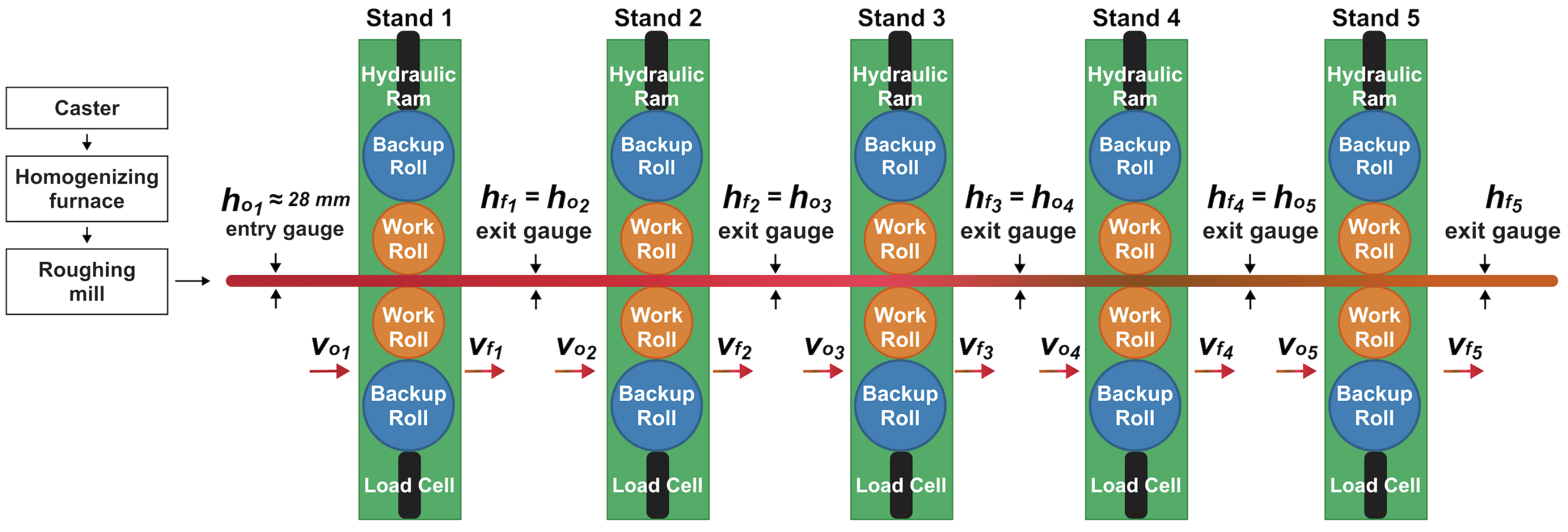
The Nucor Decatur facility features a comprehensive steelmaking operation with two continuous casters feeding a single hot rolling mill. In this process, two electric-arc steelmaking furnaces melt 150–175 ton “heats” from scrap, which are transferred to tundishes feeding two parallel casters. These casters produce 98 mm-thick slabs with varying width according to customer specifications. After reheating in tunnel furnaces to achieve temperature homogenization (typically 1100–1300 K), slabs alternate between the two production lines toward a single roughing mill where thickness is reduced to approximately 27 mm. The material then passes through a five-stand hot-finishing mill, the focus of this study, where roll forces are carefully controlled to incrementally reduce gauge to ordered specifications (Figure 1a). After exiting the final rolling stand, the steel strip is cooled along a runout table, coiled, and further processed prior to shipping to customers (Figure 1b).

Figure 2 illustrates the complete casting and rolling process at Nucor Decatur. The two parallel continuous casters alternate in feeding slabs to the single hot rolling mill with a roughing mill and five finishing stands.

3.2. Force Measurement and Control System

Each of the five roll stands consists of a pair of work rolls supported by backup rolls, which apply downward compressive force while rotating due to applied torque, which controls the exit velocity from each roll stand. The stands are equipped with load cells that continuously measure the separating forces. Force application is controlled through hydraulic systems that position the rolls to achieve specific gauge reductions. Initially, a mathematical model based on material properties, temperature, and deformation mechanics estimates required roll force. Once the first measurements of coil thickness become available, feedback control adjusts the force for the remainder of the strip to control the thickness. Any discrepancy between predicted and actual measurements informs force adjustments for subsequent coils using a machine learning algorithm.

Such an accurate real-time approach to control roll force is critical because inconsistencies in the resulting velocities and mass balance can lead to stretching of the coil between stands or rapid accumulation of steel at the next roll stand. The latter can result in a catastrophic “cobble”—a severe incident in which steel diverges from its planned route, resulting in mill damage and safety risks. Tight control of roll force, the consequent gauge, and inter-stand speed is essential to maintain proper tension as the strip becomes thinner and longer through successive stands. This ensures a consistent mass flow balance and proper tension between the stands and minimizes chatter and associated defects.

The empirical neural network models for adjusting force are only valid within specific ranges; straying outside these ranges can result in notable errors and process stability problems. Consequently, the system allows only minor adjustments in roll force between consecutive coils, necessitating minimal modifications in the machine-learning model parameters. This limitation is especially crucial in the later stands, where increased velocities can magnify any mass flow discrepancies, so gauge adjustments there must be smaller. Key process variables, including gauge changes and velocities, are given in Section 4.

3.3. Plant Measurements

Following standard data preparation procedures for regression analysis [34,35], the raw dataset underwent quality control checks to eliminate spurious data entries. A small number of observations (fewer than 10 out of nearly 40,000 data points) contained obviously erroneous values, such as negative forces, which are physically impossible in this compression process. These data entry errors were removed, resulting in the clean dataset of 38,980 measurements used throughout this study, and attached as Supplementary Material in a Datafile.

The dataset encompasses 7797 steel coils processed through the five finishing stands, yielding 38,980 individual measurements.

Table 1. Summary of Measured Variables.

Variable	Symbol	Range	Units
Entry gauge	$h_o$	1.87–35.6	mm
Exit gauge	$h_f$	1.51–27.83	mm
Roll radius	r	295–401	mm
Strip width	w	936–1720	mm
Strip temperature	T	1091–1306	K
Roll force	F	4.8–38.1	MN

summarizes the key variables recorded for each measured data “point.”

The dataset includes ten different steel grades, providing diverse material compositions for model development and validation. These grades represent a range of commercial low-carbon steel compositions, primarily varying in manganese content (0.6–1.2%), silicon (0.01–0.3%), and microalloying elements. The specific grade compositions are consistent with typical commercial hot rolled sheet products. Measurements are taken for each coil to obtain the data listed in Table 1.

Load cells embedded within the housing posts accurately measure the separating force transmitted via the backup rolls, facilitating real-time process control as explained in Section 3.2. Gauge thickness is measured by X-ray gauges, achieved by employing triangulation techniques that yield sub-millimeter measurement accuracy at the entry and exit of each stand. Velocity is measured upon exit from Stand 5, and used to calculate exit velocity from all stands, based on a mass balance with the measured gauges. The velocity entering Stand 1 was not measured in this study; thus, an average value of $1096\mathrm{mm}/\mathrm{s}$ was utilized to fit the models in this work. High-speed cameras monitor strip edges to provide real-time width measurements. Non-contact optical pyrometers monitor surface temperatures at the entry and exit of each stand. Roll radius is periodically assessed with profile gauges and this data is updated in the control system to account for wear.

3.4. Steel Grades Investigated

The dataset encompasses ten steel grades in three general groups. Plain low-carbon steels (Grades 1, 3, 7) have minimal alloying and are used for many general structural applications. Medium-carbon steels (Grades 2, 5, 8) have carbon content above the peritectic range up to 0.3% C, and therefore higher strength. Finally, HSLA steels (Grades 4, 6, 9, 10) are plain low-carbon steels which include microalloying elements (niobium, vanadium, or titanium, all <0.01%) that form carbonitride precipitates for grain refinement for applications requiring high toughness such as pipelines [36].

4. Fundamental Rolling Model Equations

This section presents the principle equations describing the mechanical relationships governing hot rolling forces, beginning with the foundational von Karman equations and progressing through equations to characterize simplified rolling mechanics and materials behavior needed for practical implementation. The variables used throughout this analysis are defined in

Table 2. Nomenclature.

Symbol	Definition	Units
	Material Properties and Stress Parameters
$\sigma$	Instantaneous flow stress	[MPa]
$\overline{\sigma }$	Mean flow stress	[MPa]
K	Strength coefficient (depends on grade, temperature, strain, and strain rate)	[MPa]
n	Strain hardening exponent	[-]
$ϵ$	True strain	[mm/mm]
$E_a$	Activation energy	[MPa·mm3/mol]
R	Universal gas constant ($8.314\times {10}^3$)	[MPa·mm3/(mol·K)]
T	Temperature	[K]
	Geometric and Force Parameters
F	Roll separating force	[MPa·mm2 = N]
		[MPa·m2 = MN]
w	Strip width	[mm]
ℓ	Contact length	[mm]
r	Roll radius	[mm]
$h_o$	Entry gauge	[mm]
$h_f$	Exit gauge	[mm]
$h_{o_1}$	Entry gauge of coil at roll Stand 1	[mm]
	Process Parameters
$\Delta t$	Contact time	[s]
v	Exit velocity	[mm/s]
${\overline{v}}_1$	Estimated mean entry velocity at Stand 1	[mm/s]
$\dot{ϵ}$	Strain rate	[s−1]
$n_{\dot{ϵ}}$	Strain rate exponent	[-]
	Model-Specific Parameters
Z	Zener–Hollomon parameter	[s−1]
A	Pre-exponential factor	[MPa]
$A_{sr}$	Strain-rate-adjusted pre-exponential factor	[MPa]
$A_i$	Pre-exponential factor for Model (Mi), $i=1,2,3$	[MPa]

.

4.1. Von Karman Equations

Governing differential equations for flat rolling were first derived by von Karman [37], by applying conditions of force equilibrium to a thin vertical slice through the roll gap. The classic von Karman equation for the distribution of normal pressure p along the roll arc is given by:

$${\displaystyle \frac{dp}{dx}}=\pm {\displaystyle \frac{2k}{\sqrt{1+{(dh/dx)}^2}}}·{\displaystyle \frac{dh}{dx}}$$

(13)

where k is the yield stress in pure shear, h is the instantaneous thickness of the material at position x along the arc of contact, and $dh/dx$ represents the thickness gradient along the roll arc [3,4]. The material flow during rolling is constrained by the roll geometry, leading to variations in pressure gradient along the arc of contact. Integrating Equation (13) along the region of contact gives the total roll force per unit width:

$${\displaystyle \frac{F}{w}}={\int }_{-\ell /2}^{\ell /2}p\left(x\right)cos\theta \left(x\right)dx$$

(14)

where $\theta \left(x\right)$ is the angle between the vertical and the normal to the roll surface at position x. Simpler models have derived from the von Karman equations [31,38] such as the widely referenced Sims’ solution [39] that forms the basis for many practical roll force models:

$$F=L·w·{\overline{Y}}_f·Q_p$$

(15)

where L is the projected length of the arc of contact, w is the strip width, ${\overline{Y}}_f$ is the mean flow stress, and $Q_p$ is a correction factor accounting for friction and inhomogeneous deformation. The relationship between the contact length ℓ and the projected length L is given by:

$$L\approx \ell cos\overline{\theta }$$

(16)

where $\overline{\theta }$ is the average angle of contact. Under typical hot rolling conditions in which the arc of contact is relatively small, L approximately equals ℓ. The correction factor $Q_p$ incorporates effects of friction, work hardening, and inhomogeneous deformation:

$$Q_p=1+{\displaystyle \frac{\mu }{k}}·{\displaystyle \frac{L}{h_{avg}}}+[\mathrm{terms}\mathrm{for}\mathrm{other}\mathrm{effects}]$$

(17)

where $\mu$ is the friction coefficient, $h_{avg}$ is the average thickness in the deformation zone, and additional terms account for factors such as work hardening. Following the approach from manufacturing texts [1,2], the roll force equation becomes:

$$F=\overline{\sigma }·w·\ell$$

(18)

where $\overline{\sigma }$ represents the effective mean flow stress that incorporates material properties, friction effects, and inhomogeneous deformation into a single term. This effective stress term $\overline{\sigma }$ captures the combined effects of the base flow stress ${\overline{Y}}_f$ and the correction factor $Q_p$ from Equation (15), such that $\overline{\sigma }={\overline{Y}}_f·Q_p$. This formulation, while maintaining the simplicity of the basic force equation, implicitly accounts for all factors affecting roll force through the empirically determined effective flow stress. It serves as the starting point for developing the statistical models in subsequent sections.

4.2. Rolling Mechanics

Hot rolling mechanics encompass intricate dynamics between the rolls and the steel strip, where the exerted forces reshape the material under carefully controlled conditions. Figure 3 demonstrates these interactions, highlighting the geometric factors and force correlations that define the rolling operation.

Because elastic strain is relatively small during the high-deformation process of hot rolling, instantaneous flow stress ($\sigma$) can be estimated from the inelastic flow strain (which combines the creep and plastic strains) as follows [40]:

$$\sigma =K{ϵ}^n$$

(19)

where K is the strength coefficient dependent on material properties and temperature, while n is the strain-hardening exponent. The mean flow stress during the entire contact length from entry to exit of the roll bite can be estimated by integrating over the strain range [40,41]:

$$\overline{\sigma }={\displaystyle \frac{1}{ϵ}}{\int }_0^{ϵ}K{\epsilon }^{n}d\epsilon ={\displaystyle \frac{K{ϵ}^n}{1+n}}$$

(20)

Substituting this expression for mean flow stress from Equation (20) into the basic roll force equation (Equation (18)), the following relationship is obtained:

$$F=\overline{\sigma }·w·\ell ={\displaystyle \frac{K{ϵ}^n}{1+n}}·w·\ell$$

(21)

This relationship combines the mean flow stress with the geometric parameters of width and contact length. However, the actual force requirements in industrial rolling depend on additional factors, particularly temperature and strain rate effects, which become increasingly important at the high temperatures and deformation rates characteristic of hot rolling operations.

4.3. Geometric and Kinematic Relationships

During hot rolling, the material undergoes both geometric and kinematic changes as it passes through the rolls. The contact length between the material and roller represents a critical parameter influencing force requirements. This length is determined by the geometry of the region where the metal is in contact with the rolls (as shown in Figure 3b) [1,2]:

$$\ell =\sqrt{r(h_o-h_f)}$$

(22)

where r is the roll radius, $h_o$ is the entry gauge, and $h_f$ is the exit gauge at a given roll stand.

The strain experienced by the material during rolling is approximated by the simple relationship [40]:

$$ϵ=ln\left({\displaystyle \frac{h_o}{h_f}}\right)$$

(23)

This logarithmic strain measure accounts for the true deformation during the thickness reduction process and length expansion.

The velocity of the material varies through the roll gap due to conservation of mass. As the material thickness decreases, its velocity must increase proportionally. This relationship follows from mass conservation [2]:

$$v={\overline{v}}_1·{\displaystyle \frac{h_{o_1}}{h_f}}$$

(24)

where v is the exit velocity at a given stand, ${\overline{v}}_1$ is the estimated mean velocity into the first stand, $h_{o_1}$ is the entry gauge into the first stand, and $h_f$ is the exit gauge from the current stand. In the regression analysis in this work, the reference velocity ${\overline{v}}_1$ was set to an estimated value of 1096 mm/s based on typical mill operating conditions. Similarly, $h_{o_1}$ was set to the average value of 25.8 mm for all 7797 coils in the dataset. With a standard deviation of only 2 mm, variations in these reference values had no significant effect on force prediction. This velocity relationship has important implications for the strain rate during rolling. The contact time between the material and rolls is estimated by:

$$\Delta t={\displaystyle \frac{\ell }{v}}$$

(25)

Combining Equations (23) and (25) allows for the calculation of the strain rate during rolling:

$$\dot{ϵ}={\displaystyle \frac{ϵ}{\Delta t}}=ln\left({\displaystyle \frac{h_o}{h_f}}\right)·{\displaystyle \frac{v}{\ell }}$$

(26)

These geometric and kinematic relationships provide the foundation for quantitative approximation of the deformation process during hot rolling and form essential inputs to the force prediction models.

4.4. Material Behavior During Hot Rolling

Steel undergoes complex deformation during hot rolling, with its response governed by metallurgical characteristics that vary across different grades according to microstructural phenomena at the grain scale and below. The material response includes elastic and inelastic (plastic and creep) strain. In hot rolling processes, the elastic strain is negligible. So, treating inelastic strain as a single term gives rise to a power-law approximation relating stress and strain [40,41], as shown in Equation (19).

The strength coefficient exhibits temperature dependence through an Arrhenius-type relationship [42]:

$$K=A·e^{{\displaystyle \frac{E_a}{RT}}}$$

(27)

where A is the pre-exponential factor, $E_a$ is the activation energy, R is the universal gas constant, and T is the absolute temperature. This equation applies generally to all temperature conditions, not just isothermal cases. However, at high deformation rates in commercial rolling, strain rate effects become significant [2]. Following the approach of Sellars and McTegart [42] and subsequent researchers, the combined effects of temperature and strain rate are captured through the Zener–Hollomon parameter [43]:

$$Z=\dot{ϵ}·e^{{\displaystyle \frac{E_a}{RT}}}$$

(28)

The strength coefficient including strain rate effects becomes:

$$K=A_{sr}·Z^{n_{\dot{ϵ}}}=A_{sr}·{\left[\dot{ϵ}·e^{{\displaystyle \frac{E_a}{RT}}}\right]}^{n_{\dot{ϵ}}}$$

(29)

where $A_{sr}$ is the strain-rate-adjusted pre-exponential factor and $n_{\dot{ϵ}}$ is the strain rate sensitivity exponent. Note that $A_{sr}$ differs from A because it incorporates the strain rate sensitivity of the material. Expanding Equation (29):

$$K=A_{sr}·{\dot{ϵ}}^{n_{\dot{ϵ}}}·e^{{\displaystyle \frac{n_{\dot{ϵ}}{E}_a}{RT}}}$$

(30)

The appearance of $n_{\dot{ϵ}}{E}_a$ in the exponential term has been debated in the literature. Some researchers [42,43] maintain both parameters separately to preserve their physical meaning, while others combine them into an effective activation energy $E_{eff}=n_{\dot{ϵ}}{E}_a$ for simplicity [11]. This work maintains them separately to facilitate physical interpretation. Substituting this expression for K into the mean flow stress equation (Equation (20)) yields:

$$\overline{\sigma }={\displaystyle \frac{K{ϵ}^n}{1+n}}={\displaystyle \frac{A_{sr}}{1+n}}·{\dot{ϵ}}^{n_{\dot{ϵ}}}·e^{{\displaystyle \frac{n_{\dot{ϵ}}{E}_a}{RT}}}·{\left[ln\left({\displaystyle \frac{h_o}{h_f}}\right)\right]}^n$$

(31)

4.5. Final Roll Force Physical Model

Inserting the mean flow stress expression (Equation (31)) into the basic roll force equation (Equation (18)) gives a comprehensive physical model for roll force:

$$F=\overline{\sigma }·w·\ell ={\displaystyle \frac{A_{sr}}{1+n}}·{\dot{ϵ}}^{n_{\dot{ϵ}}}·e^{{\displaystyle \frac{n_{\dot{ϵ}}{E}_a}{RT}}}·{\left[ln\left({\displaystyle \frac{h_o}{h_f}}\right)\right]}^n·w·\ell$$

(32)

This equation accounts for:

• Material properties through $A_{sr}$, n, and $n_{\dot{ϵ}}$
• Temperature effects through the Arrhenius term $e^{{\displaystyle \frac{n_{\dot{ϵ}}{E}_a}{RT}}}$
• Strain rate effects through ${\dot{ϵ}}^{n_{\dot{ϵ}}}$
• Strain hardening through ${\left[ln\left({\displaystyle \frac{h_o}{h_f}}\right)\right]}^n$
• Geometric factors through width w and contact length ℓ

The model presented in Equation (32) is similar to equations used in previous literature, and forms the basis for the statistical models developed in this work.

5. Visualization of Process Variable Relationships

The relationships between forces, stresses, and process variables from the commercial hot rolling process in the 38,980 data points uncover significant patterns that guide the modeling methodology. Identifying these connections is crucial to building statistical models of the hot rolling process.

Table 3. Variable statistics (mean ± standard deviation) across roll stands.

Variable	Stand 1	Stand 2	Stand 3	Stand 4	Stand 5	Overall
Measured Variables
Entry gauge [mm]	25.8 ± 2.1	18.2 ± 2.0	12.4 ± 1.8	8.5 ± 1.5	5.8 ± 1.2	14.1 ± 7.4
Exit gauge [mm]	18.2 ± 2.0	12.4 ± 1.8	8.5 ± 1.5	5.8 ± 1.2	4.0 ± 0.9	9.8 ± 5.6
Roll diameter [mm]	775 ± 45	760 ± 42	745 ± 40	730 ± 38	715 ± 35	745 ± 44
Width [mm]	1285 ± 185	1285 ± 185	1285 ± 185	1285 ± 185	1285 ± 185	1285 ± 185
Temperature [K]	1265 ± 18	1242 ± 17	1220 ± 16	1198 ± 16	1176 ± 15	1220 ± 38
Roll Force [MN]	24.2 ± 3.8	20.5 ± 3.2	17.1 ± 2.8	14.2 ± 2.4	11.8 ± 2.1	17.6 ± 5.4
Calculated Variables
Entry velocity [mm/s]	1096	1670 ± 185	2450 ± 350	3570 ± 520	5240 ± 780	2822 ± 1480
Exit velocity [mm/s]	1670 ± 185	2450 ± 350	3570 ± 520	5240 ± 780	7590 ± 1120	4104 ± 2150
Contact length [mm]	22.5 ± 2.8	18.2 ± 2.3	14.8 ± 2.0	11.5 ± 1.6	8.9 ± 1.3	15.2 ± 5.3
Contact time [s]	0.015 ± 0.004	0.008 ± 0.002	0.004 ± 0.001	0.002 ± 0.001	0.001 ± 0.0004	0.006 ± 0.005
Strain [mm/mm]	0.35 ± 0.06	0.38 ± 0.05	0.42 ± 0.05	0.45 ± 0.05	0.48 ± 0.06	0.42 ± 0.08
Strain rate [s−1]	35 ± 12	68 ± 22	142 ± 48	285 ± 95	520 ± 180	210 ± 195
Stress [MPa]	135 ± 22	162 ± 26	185 ± 30	208 ± 34	235 ± 38	185 ± 45

shows the ranges of both the measured and calculated process variables across the five roll stands. As characterized by standard deviation, the ranges generally indicate bigger differences between roll stands than within each roll stand. Gauge, temperature, force, contact length and contact time all decrease between stands, while stress, strain, and strain rate all consistently increase with stand.

5.1. Force and Stress vs. Temperature

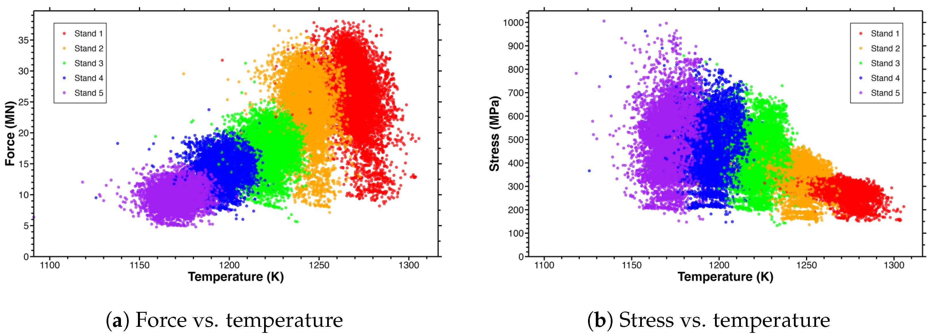
Plotting all of the data in Figure 4 shows the relationships between temperature and both force and stress across all five stands. In Figure 4a, each stand exhibits a clear, although weak, expected trend of decreasing force with increasing temperature within each stand. However, combining the data across all stands shows the opposite trend: Stand 1 operates at the highest temperatures and forces, while Stand 5 operates at the lowest temperatures and forces.

Figure 4b shows that stress levels consistently increase from Stand 1 to Stand 5. This trend aligns with known material behavior, in which flow stress increases with decreasing temperature. However, the increase may not appear to be as much as expected. Furthermore, within each stand, the trend is not clear. This unexpected behavior is due to plant practices designed to balance forces and to avoid excessive force in any stand. This gives rise to opposing trends for other process variables, discussed in the next sections.

5.2. Force and Stress vs. Strain

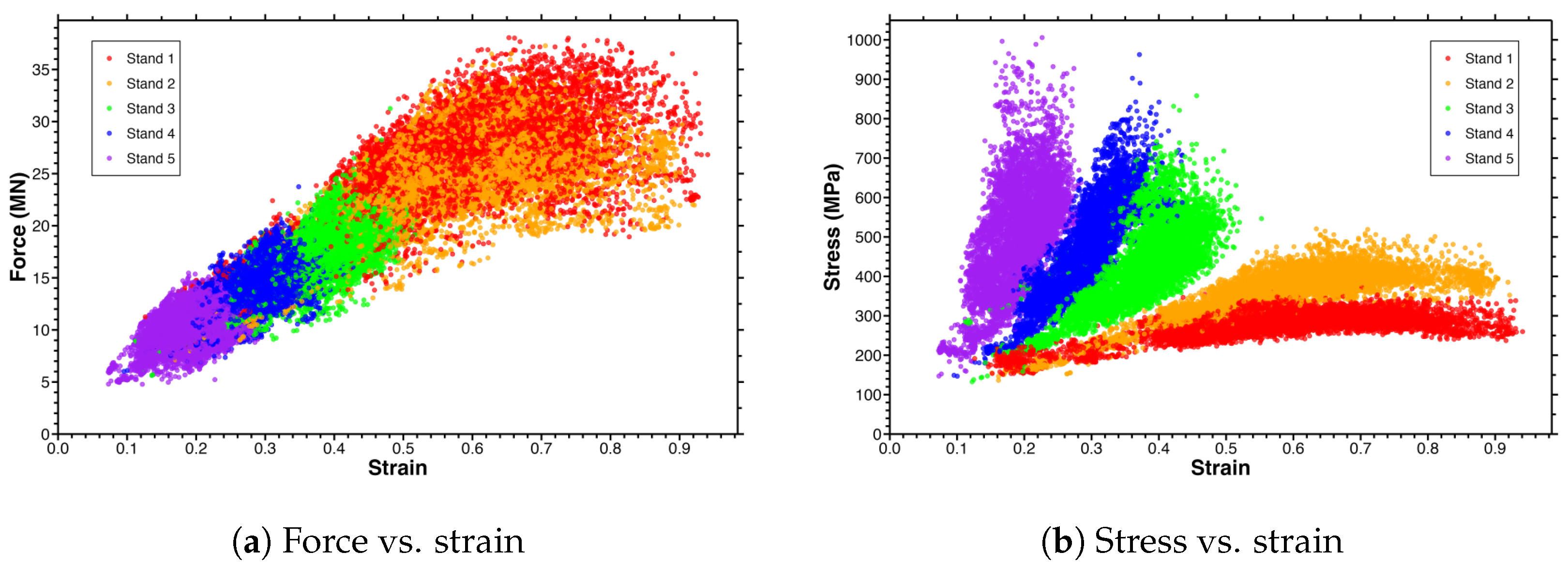
Figure 5 presents the relationships between strain and both force and stress. In Figure 5a, the data reveals clustering by stand, with force increasing almost proportionally with strain. Stand 1 operates at the highest strains and forces, demonstrating the mill’s approach of larger gauge reductions in early stands, where velocity is lower, stability is higher, and tolerances are not as critical.

In Figure 5b, stress clearly increases with strain within each stand. In Stand 1, stress is low, even at high strain, while stress increases greatly with strain in Stand 5. This matches expectations of material behavior, considering the effect of strength increasing with strain, especially at lower temperatures. However, the overall trend of stress variation between stands is not as clear. This is because strain decreases greatly with stand. These effects of decreasing strain and increasing stress with decreasing temperature, which occur between stands, tend to counter the expected increases in stress and force.

5.3. Force and Stress vs. Contact Length

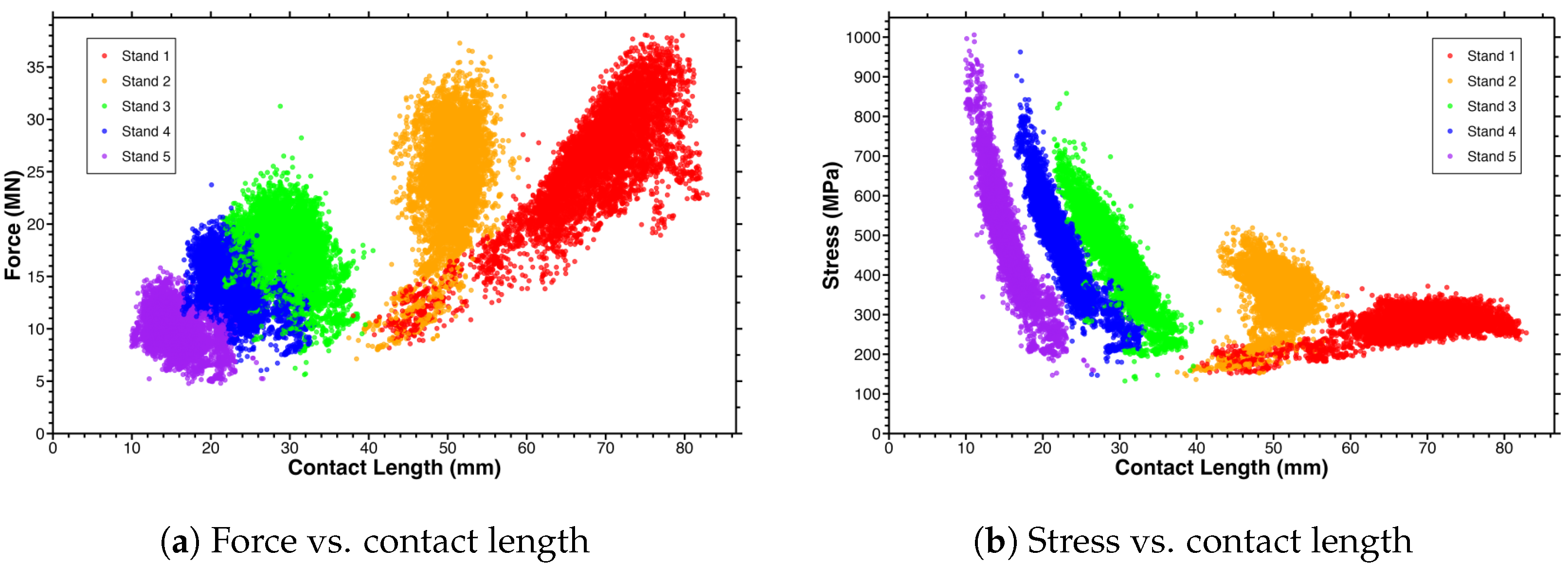
Figure 6 illustrates the relationships between contact length and both force and stress. Contact length naturally tends to decrease with stand, owing to the increase in strength with decreasing temperature. The relationships with force and stress are complicated, however. In Figure 6a, the overall trend across stands shows force increasing with contact length as expected, for a given material flow stress. The data forms distinct clusters for each stand, progressing from Stand 1 (highest forces and contact lengths) to Stand 5 (lowest forces and contact lengths).

In Figure 6b, stress in Stand 1 increases with contact length, as expected due to strain hardening. By contrast, stress in Stands 3–5 clearly decreases with contact length. The latter is likely due to the plant practice of maintaining reasonably constant force within the stand. When the steel is stronger (higher flow stress), this practice requires less strain, which needs less thickness reduction, which also shortens contact length.

5.4. Force and Stress vs. Width

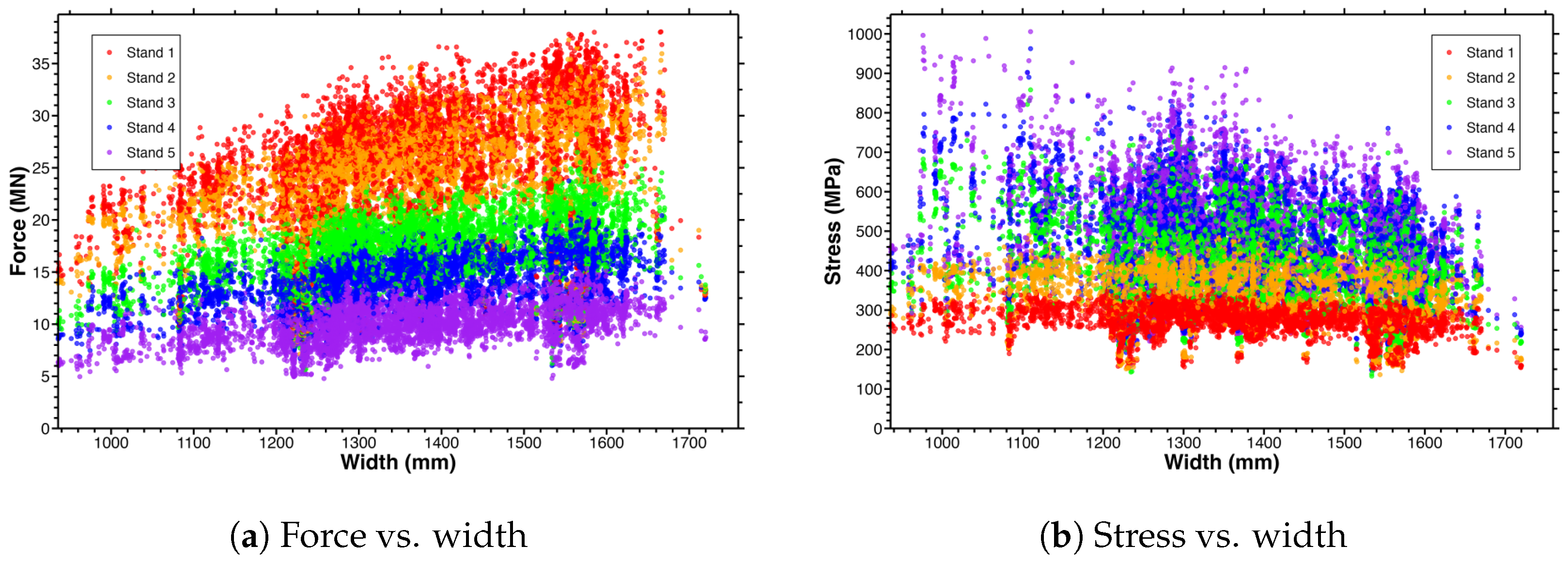
Figure 7 shows the relationships between strip width and both force and stress. In Figure 7a, force naturally increases linearly in direct proportion with width. This supports treating width as a fundamental geometric variable in the models according to Equation (18).

In Figure 7b, the data shows higher stress with increasing stand (from Stand 1 to Stand 5), which is likely attributable to the increasing strain rate as the steel progresses through the mill. The expectation of stress staying constant with width is not quite satisfied. Interestingly, in Stand 5, stress appears to decrease slightly with increasing width.

5.5. Force and Stress vs. Strain Rate

Figure 8 shows the effect of strain rate on both force and stress. In Figure 8a, within each stand, force increases greatly with strain rate, especially in the early stands. The sensitivity of force to strain rate decreases with successive stands, as evidenced by the progressively shallower slopes from Stand 1 to Stand 5, perhaps due to cumulative work hardening from prior deformation. In Figure 8b, stress increases with strain rate due to classic hardening behavior. Stand 1 operates at lower strain rates with lower stress levels, whereas subsequent stands operate at progressively higher strain rates with correspondingly higher stress levels.

5.6. Key Insights from Visualization

The data visualization reveals several critical patterns that inform the modeling approach. There is a strong cross-correlation between temperature, strain and contact length with stand position. As steel progresses through the stands, temperature decreases, which tends to increase stress and force; both strain and contact length decrease, which tends to decrease force. These offsetting trends are due to operational strategy, as mentioned earlier. This creates statistical relationships that can obfuscate the true physical relationships between individual variables when analyzed across all stands simultaneously. For example, within individual stands, force generally decreases with increasing temperature (as expected from material softening). However, when all stands are analyzed together, the opposite trend appears due to the operational strategy of applying higher forces at earlier, hotter stands. Force increases approximately linearly with width. The consistent influence of strain rate increasing both force and stress suggests that strain rate is likely to be well behaved in the statistical models.

6. Regression Model Formulation

Based on the insights gained from data visualization, a series of regression models have been developed by fitting the roll-force measurement data to different simplifications of the classic rolling equations presented in Section 4. Following standard regression modeling methodology [34,35,44], the approach involves: selection of the model equation, variable transformations, linear regression analysis, back-transformation, statistical evaluation, and validation with training and testing datasets. This aims to balance model accuracy with practical utility, addressing the cross-correlation challenges identified in the visualization phase.

To employ linear regression methods, the nonlinear equations in Section 4 are converted into the following linear form using a logarithmic transformation:

$$lnF={\beta }_0+{\beta }_1{X}_1+{\beta }_2{X}_2+{\beta }_3{X}_3+{\beta }_4{X}_4$$

(33)

where F is the predicted force from $X_i$, $X_i$ are the variables from the measured data, and ${\beta }_i$ are the fitted parameters resulting from the regression analysis. Linear regression was performed on this equation using least squares minimization [45] to find best-fit values of the beta parameters. These fitted parameters are then converted back into their corresponding physical parameters.

The initial comprehensive model (Model M0) includes temperature, strain, strain rate, and geometric factors. This is Equation (32) in which variation is permitted in the exponents for width and contact length:

$$F={\displaystyle \frac{A_{sr}}{n+1}}·{\left[\dot{ϵ}·e^{{\displaystyle \frac{E_a}{RT}}}\right]}^{n_{\dot{ϵ}}}·{\left[ln\left({\displaystyle \frac{h_o}{h_f}}\right)\right]}^n·w^{{\beta }_w}·{\ell }^{{\beta }_{\ell }}$$

(34)

Inserting the strain rate $\dot{ϵ}$, which is estimated from strain and deformation time period in Equation (26), and from the contact length, which is evaluated with Equation (22), Equation (34) becomes:

$$F={\displaystyle \frac{A_{sr}}{n+1}}·{\left[ln\left({\displaystyle \frac{h_o}{h_f}}\right)·{\displaystyle \frac{1}{\ell }}·\left({\overline{v}}_1·{\displaystyle \frac{h_{o_1}}{h_f}}\right)·e^{{\displaystyle \frac{E_a}{RT}}}\right]}^{n_{\dot{ϵ}}}·{\left[ln\left({\displaystyle \frac{h_o}{h_f}}\right)\right]}^n·w^{{\beta }_w}·{\ell }^{{\beta }_{\ell }}$$

(35)

Applying logarithms to Equation (35) and reformulating the expression gives:

$$\underset{F^{*}}{\underbrace{lnF}}=\underset{{\beta }_0}{\underbrace{ln\left({\displaystyle \frac{A_{sr}}{n+1}}\right)}}+\underset{{\beta }_1}{\underbrace{n_{\dot{ϵ}}}}·\underset{X_1}{\underbrace{\left[{\displaystyle \frac{E_a}{RT}}+ln\left({\overline{v}}_1·{\displaystyle \frac{h_{o_1}}{h_f}}\right)+lnϵ-ln\ell \right]}}+\underset{{\beta }_2}{\underbrace{n}}·\underset{X_2}{\underbrace{lnϵ}}+\underset{{\beta }_3}{\underbrace{1}}·\underset{X_3}{\underbrace{lnw}}$$

$$+\underset{{\beta }_4}{\underbrace{1}}·\underset{X_4}{\underbrace{ln\ell }}$$

(36)

After performing the linear regression, the fitted regression coefficients (${\beta }_i$) are transformed back to the physical parameters in the original model (Equation (34)) as follows:

$$\begin{array}{cc}\hfill A_{sr}& =(n+1)·e^{{\beta }_0}\hfill \end{array}$$

(37)

$$\begin{array}{cc}\hfill n_{\dot{ϵ}}& ={\beta }_1\hfill \end{array}$$

(38)

$$\begin{array}{cc}\hfill n& ={\beta }_2\hfill \end{array}$$

(39)

$$\begin{array}{cc}\hfill {\beta }_w& ={\beta }_3\hfill \end{array}$$

(40)

$$\begin{array}{cc}\hfill {\beta }_{\ell }& ={\beta }_4\hfill \end{array}$$

(41)

Note that the strain-rate-adjusted pre-exponential factor $A_{sr}$ requires the strain hardening exponent n (${\beta }_2$) for its calculation. The activation energy $E_a$ is embedded within the temperature-dependent term within $X_1$ and cannot be independently determined from this linear regression approach.

Although seemingly comprehensive, Model M0 yielded an $R^2$ value of 0.61 for the combined model over all coils (0.65 to 0.85 for specific grade models). Even more concerning were the trends that contradicted physical expectations: the model suggested that force rose with increasing temperature, and the exponents for width and contact length varied greatly from their anticipated value of 1. This poor performance is attributed to the high correlation among strain, temperature, and roll stand position in industrial hot rolling processes. The manufacturing facility intentionally controls strain for each coil and with roll stand to maintain an even distribution of forces. This approach, together with the inherent temperature decrease between stands and its effect on material strength, results in less strain and shorter contact lengths as the coils advance through the stands. Furthermore, the decrease in gauge causes the velocity and accompanying strain rate to increase with increasing stand. These interrelated factors create notable cross-correlations that counteract some of the expected physical behavior, resulting in coefficients in the regression model that are not physically realistic, particularly concerning activation energy ($E_a/R$) and the strain hardening exponent (n). Considering these difficulties, Model M0 was set aside in favor of simpler alternatives aimed at reducing the adverse impacts of these cross-correlations while maintaining predictive accuracy.

7. Combined Models

This section presents linear regression results of three simple “combined models” applied to the entire dataset of 7797 coils and 38,980 data points, combining all ten steel grades. These models are simplifications of Model M0 and were evaluated using the same logarithmic methodology for the linear regression analysis described in Section 6.

7.1. Model M1: Temperature-Dependent Strain Rate Model

Model M1 eliminates the strain hardening term in Model M0 while keeping the effects of temperature and strain rate:

$$F=A_1·{\dot{ϵ}}^{n_{\dot{ϵ}}}·e^{\left({\displaystyle \frac{E_a}{RT}}\right)n_{\dot{ϵ}}}·w^{{\beta }_w}·{\ell }^{{\beta }_{\ell }}$$

(42)

where $A_1$ represents a model-specific coefficient that includes strain hardening and other neglected terms in Model M0. This combined model yields:

$$F\left[\mathrm{N}\right]=1270.3·\dot{ϵ}{\left[{\mathrm{s}}^{-1}\right]}^{0.305}·e^{(-2207/T[\mathrm{K}\left]\right)·0.305}·w{\left[\mathrm{mm}\right]}^{0.971}·\ell {\left[\mathrm{mm}\right]}^{0.895}$$

(43)

This reveals a negative temperature coefficient ($E_a/R=-2207$ K), which contradicts metallurgical principles for hot steel deformation, where positive values around 200,000 to 400,000 K are expected [9,46]. This inconsistency stems from the cross-correlation between temperature, strain distribution, contact length, and roll stand position in the commercial rolling process. Despite achieving a strong fit (R² = 0.948), this physically unrealistic temperature coefficient makes Model M1 unsuitable for further analysis.

7.2. Model M2: Strain Rate Model

Based on the temperature coefficient complications identified in Model M1, Model M2 removes the temperature component but maintains the influence of strain rate:

$$F=A_2·{\dot{ϵ}}^{n_{\dot{ϵ}}}·w^{{\beta }_w}·{\ell }^{{\beta }_{\ell }}$$

(44)

where $A_2$ consolidates temperature and other influencing factors into a unified coefficient. This model achieves the following fitted equation:

$$F\left[\mathrm{N}\right]=154.5·\dot{ϵ}{\left[{\mathrm{s}}^{-1}\right]}^{0.310}·w{\left[\mathrm{mm}\right]}^{0.963}·\ell {\left[\mathrm{mm}\right]}^{0.992}$$

(45)

The geometric coefficients are close to their expected values, with width and contact length exponents near 1.0, demonstrating that the model is reasonable. This model achieves very good fit ($R^2=0.947$) with only a 0.19% decrease in $R^2$ compared to Model M1.

7.3. Model M3: Simplified Strain Rate Model

Model M3 enforces the physical expectation from the force–stress relationship that ${\beta }_w$ and ${\beta }_{\ell }$ should be 1, giving rise to the following equation:

$$F=A_3·{\dot{ϵ}}^{n_{\dot{ϵ}}}·w·\ell$$

(46)

where $A_3$ denotes the mean flow stress coefficient, encompassing all material characteristics and processing conditions except strain rate. This approach reduces the fitting parameters to two while maintaining physical consistency with rolling theory:

$$F\left[\mathrm{N}\right]=113.1·\dot{ϵ}{\left[{\mathrm{s}}^{-1}\right]}^{0.314}·w\left[\mathrm{mm}\right]·\ell \left[\mathrm{mm}\right]$$

(47)

The strain rate exponent of 0.314 characterizes the material response across all ten grades, providing a unified description of steel behavior during hot rolling. This model achieves $R^2$ = 0.946, which is almost the same as that of the four-parameter Model M2. Expanding the strain rate and contact length terms gives the following final Model M3, for practical implementation:

$$F\left[\mathrm{N}\right]=113.1·{\left[ln\left({\displaystyle \frac{h_o}{h_f}}\right)·{\displaystyle \frac{v}{\sqrt{r(h_o-h_f)}}}\right]}^{0.314}·w·\sqrt{r(h_o-h_f)}$$

(48)

where $h_o$ is entry gauge [mm], $h_f$ is exit gauge [mm], v is exit velocity [mm/s] from the stand, r is roll radius [mm], and w is strip width [mm]. This expanded form allows direct calculation of roll force from the five readily available rolling process variables.

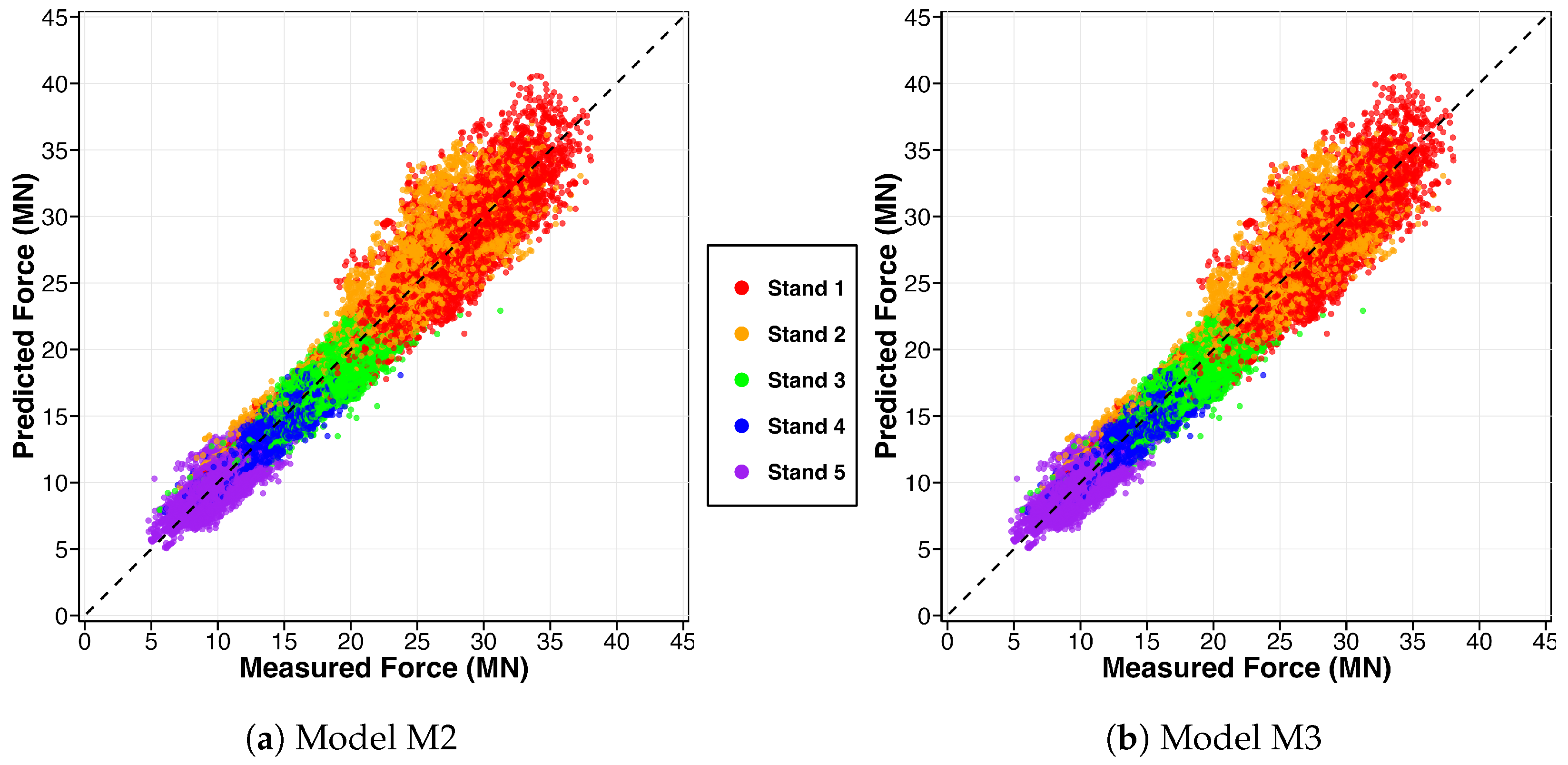
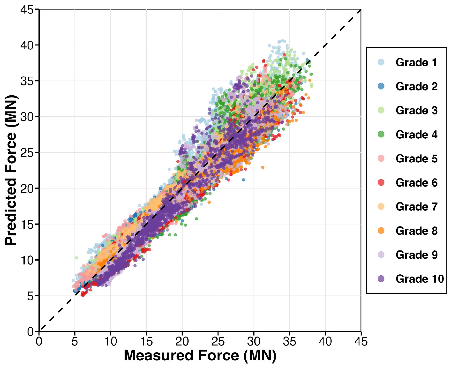
Figure 9 illustrates the performance of Models M2 and M3 grouped according to stand. Both models show acceptable prediction capability for a large industrial database. Figure 10 illustrates the performance of Model M3 grouped according to grade. The dashed diagonal line represents perfect prediction. Retaining high $R^2$ after simplification from four parameters in Model M2 to two parameters in Model M3 shows that enforcing the expected physical behavior is a good simplification. Thus, model M3 is recommended as the best combined model of this work.

Next, the generality of these combined models is checked with a train–test validity analysis. Then, the benefit of accounting for the effects of varying strengths between steel grades is investigated.

7.4. Train–Test Split Model Validation

Following standard validation practices in regression analysis [34,44], model validation is performed to ensure that the models can reliably predict unseen data rather than simply overfitting to the training dataset. The complete dataset ($n=38,980$ measurements) was randomly partitioned into training (80%, $n=31,184$) and testing (20%, $n=7796$) subsets using a random seed for reproducibility. The three combined models just presented were refitted using only the training data, and performance was evaluated on both the training and testing sets to assess generalization capability.

Model performance is assessed using two complementary metrics: (1) the coefficient of determination ($R^2$), which measures the proportion of variance explained by the model; and (2) the root mean square error (RMSE), which quantifies the average magnitude of prediction errors in the units (MN) of the response variable, force.

Table 4. Train-test validation of combined model performance on training and testing datasets.

Model	${\mathit{R}}^2$		Root Mean Square Error (MN)
(Combined Grade)	Training Data	Testing Data	Training Data	Testing Data
M1	0.949	0.948	1.61	1.60
M2	0.947	0.946	1.65	1.64
M3	0.945	0.945	1.66	1.65

summarizes the results.

All three models demonstrate excellent generalization, with testing values of $R^2$ within 0.001 of training values and testing values of RMSE within 0.01 MN of training values. This minimal performance degradation on unseen data indicates that the models are fitting general behavior in the data rather than overfitting to mask noise in the training data. Furthermore, both training and testing models roughly match the original models presented in the previous section.

However, strong statistical performance alone does not ensure a good model. Model M1, despite its excellent statistical metrics, was rejected in Section 7.1 due to its physically unrealistic negative temperature coefficient. Model M3, despite its simplified structure with only 2 fitted parameters, maintains performance equivalent to the more complex Model M2 (4 fitted parameters) on both training and testing datasets while also satisfying physically logical constraints.

This validation analysis provides strong evidence that Model M3 should perform reliably when applied to new rolling campaigns with similar steel grades and process conditions, combining both statistical validity and physically logical behavior.

8. Grade-Specific Models

This section applies the simplified Models M2 and M3 in Equations (44) and (46), respectively, to fit separate regression equations for each of the ten steel grades in this study. Each grade-specific model was fit from the subset of the database for coils of just that one grade. Results for all ten grade-specific models are provided in

Table 5. Grade-specific Model M2 Results.

Grade	# of Coils	Data Points	${\mathit{A}}_2$	${\mathit{n}}_{\dot{\mathit{ϵ}}}$	${\mathit{\beta }}_{\mathit{w}}$	${\mathit{\beta }}_{\mathit{\ell }}$	${\mathit{R}}^2$
1	2254	11,270	91.61	0.322	0.991	1.055	0.967
2	1543	7710	213.56	0.356	0.880	1.032	0.972
3	1182	5910	154.36	0.303	0.947	1.027	0.974
4	760	3800	208.50	0.267	1.017	0.864	0.965
5	392	1960	107.70	0.395	0.916	1.107	0.972
6	372	1860	81.53	0.290	1.131	0.872	0.977
7	335	1675	621.49	0.294	0.759	1.028	0.978
8	333	1665	113.84	0.325	0.982	1.043	0.983
9	320	1600	1247.30	0.216	0.827	0.799	0.954
10	306	1530	665.27	0.215	0.926	0.780	0.967
Total	7797	38,980

and

Table 6. Grade-specific Model M3 Results.

Grade	# of Coils	Data Points	${\mathit{A}}_3$	${\mathit{n}}_{\dot{\mathit{ϵ}}}$	${\mathit{R}}^2$
1	2254	11,270	117.6	0.291	0.958
2	1543	7710	103.6	0.346	0.970
3	1182	5910	122.6	0.288	0.967
4	760	3800	108.2	0.342	0.938
5	392	1960	94.9	0.362	0.971
6	372	1860	102.2	0.364	0.958
7	335	1675	123.1	0.285	0.969
8	333	1665	130.3	0.295	0.976
9	320	1600	103.8	0.344	0.907
10	306	1530	102.6	0.353	0.912
Total	7797	38,980

for Models M2 and M3 respectively, along with their performance, as indicated by $R^2$.

For example, inserting the parameter values from Table 6 for Grade 2 (comprising 1540 coils and 7700 data points) gives the following grade-specific Model M3:

$$F\left[\mathrm{N}\right]=103.6·\dot{ϵ}{\left[{\mathrm{s}}^{-1}\right]}^{0.346}·w\left[\mathrm{mm}\right]·\ell \left[\mathrm{mm}\right]$$

(49)

The strain rate exponent ($n_{\dot{ϵ}}$) in Model M3 varies systematically with steel composition. Low-carbon grades (1, 2, 3, 7, 8) exhibit values ranging from 0.285 to 0.346, medium-carbon grades (4, 5, 6) show consistently higher values from 0.342 to 0.364, while microalloyed grades (9, 10) fall in between at 0.344 and 0.353. The two highest strain rate exponents occur in the medium-carbon grades 6 (0.364) and 5 (0.362), indicating greater strain rate sensitivity in these higher-strength steels [47]. This systematic trend reflects the expected strengthening mechanisms: medium-carbon grades show enhanced strain rate sensitivity due to their higher carbon content and associated dislocation interactions, while the microalloyed grades exhibit intermediate behavior due to precipitation strengthening effects that partially restrict dynamic recovery [48,49]. The width coefficients lie close to 1 for Model M2, indicating that force increases linearly with width. The contact length exponents show greater variation than the width exponents. The reasonable behavior of the width and length exponents extends to every grade-specific Model M2, which further validates the formulation of Model M3. As expected, the grade-specific models show better performance than the combined models, with $R^2$ values ranging from 0.954 to 0.983 over the 10 grades for Model M2. Model M3 achieves similar performance in terms of fit, with $R^2$ values ranging from 0.948 to 0.981.

Figure 11 shows the performance of the grade-specific models M2 and M3, colored by stand. These predicted-vs.-measured force plots reveal distinct clustering patterns across different stands. In the early stands (Stands 1–2), where processing temperatures are higher, the data points exhibit greater scatter and separation between force levels. By contrast, the later stands (Stands 3–5), operating at lower strains and contact lengths, show more tightly clustered and uniform force predictions. This strain-dependent clustering pattern suggests that model accuracy improves as the range of deformation differences between coils lessens.

Comparing Figure 10 (combined Model M3) with Figure 12 (grade-specific M3 models), indicates only a slight variation in fit. The grade-specific models offer only minor enhancements in $R^2$ values despite their greatly increased complexity (from 2 to 20 estimated parameters). All models demonstrate consistent cross-correlation effects between temperature, strain, and stand position, affirming that these observed trends are intrinsic to the multi-stand rolling process, rather than being related to some steel grade effect. This observation supports the use of the simpler combined model with only two parameters for practical applications across all steel grades.

9. Discussion

This section explores the implications of the statistical models of roll force just presented. The three models, as applied to both the complete data set and each individual grade, are further compared and evaluated. The best model is then tested against other roll force measurements in previous literature to assess its wider applicability. Finally, the practical implications of this study are discussed, focusing on how the natural cross-correlations in multi-stand hot rolling operations strongly affect statistical analyses of this industrial process.

9.1. Model Selection

Table 7. Model Performance: Comparison of $R^2$ values.

Grade	M1	M2	M3
	Combined Models
-	0.948	0.947	0.946
	Grade-Specific Models
1	0.972	0.967	0.963
2	0.972	0.972	0.970
3	0.977	0.974	0.971
4	0.966	0.965	0.961
5	0.973	0.972	0.970
6	0.977	0.977	0.974
7	0.978	0.978	0.975
8	0.983	0.983	0.981
9	0.961	0.954	0.948
10	0.970	0.967	0.962

compares the performance of all three models developed in this study, including both combined and grade-specific models, based on $R^2$ values. All models show strong fit for big data analysis of industrial measurements, with $R^2$ consistently exceeding 0.94. Model M1 achieves marginally higher $R^2$ than Models M2 and M3; however, this minimal improvement (less than 0.002) does not justify the additional complexity of including temperature as a variable. Moreover, the temperature coefficient in M1 exhibits negative correlation with force, contradicting metallurgical expectations that flow stress increases with decreasing temperature. This physically implausible relationship occurs for both the combined model and all grade-specific models, leading us to reject Model M1.

Among the two viable models remaining, Model M2 achieves a slightly better fit with $R^2$ = 0.947 and fitted geometric coefficients (${\beta }_w$ = 0.963 and ${\beta }_{\ell }$ = 0.992) that deviate slightly from 1.0. While these deviations marginally improve statistical fit, they lack physical significance. Conversely, Model M3 sets both geometric coefficients to exactly 1, aligning with fundamental rolling theory while negligibly sacrificing fit ($R^2$ = 0.946, a difference of only 0.001). This constraint reduces the model to just two parameters (coefficient $A_3$ and strain rate exponent $n_{\dot{ϵ}}$) compared to M2’s four parameters, significantly simplifying parameter estimation and interpretation.

Crucially, Model M3’s formulation with geometric exponents of 1.0 enables direct stress prediction by dividing both sides of Equation (46) by the contact area ($w·\ell$), yielding a physically meaningful relationship between stress and strain rates. This theoretical consistency, combined with virtually identical predictive performance to M2, makes M3 particularly attractive for practical applications.

The grade-specific models show minimal improvement over the combined models (average $R^2$ increase less than 0.02), suggesting that the additional complexity of maintaining ten separate models and requiring prior knowledge of steel grade classification is not justified for most applications. Despite the clear grade-based clustering visible in Figure 12, the combined Model M3 captures the essential rolling behavior with a single strain rate exponent and coefficient, achieving $R^2$ = 0.946 across all grades. This combination of theoretical soundness, parameter parsimony, and fit similar to Model M2 makes Model M3 the recommended choice for practical use.

9.2. Comparison with Previous Literature

The best model, the simplified strain rate model M3, was further evaluated by comparing its predictions with force measurements from previous literature. Kumar et al. [18] conducted Gleebel-3500 tests at temperatures of 1132–14,132 K, entry gauges of 18–250 mm, and a roller diameter of 1095 mm, at strain rates of 0.2–0.9 s⁻¹, which is substantially lower than the 100–400 s⁻¹ typical of commercial hot rolling. Model M3 predictions of the roll force over 14 sets of their measurements produced an average error of −17%. Yilmaz et al. [50] measured roll force during hot rolling of low-carbon steel in a commercial rebar mill, processing 150 mm square billets at 1323–1423 K with 420 mm diameter rollers at a strain rate of 0.32 s⁻¹. Model M3 predictions had an average error of +11% over 6 sets of their measurement data. Despite these studies not involving coil rolling and with much lower strain rates than typical of commercial hot rolling such as the current study, Model M3 predictions showed a reasonable match with the measurements, demonstrating its applicability even beyond its calibration dataset domain.

9.3. Practical Implications

The success of Model M3, which omits specific terms for temperature and strain, is attributed to the intrinsic cross-correlations present in commercial multi-stand rolling processes. As the steel moves through the series of five finishing stands, its temperature naturally cools from roughly 1265 K to 1176 K. Concurrently, to prevent equipment overload and to achieve uniform force distribution, operators reduce the gauge at each successive stand. This operational practice consequently causes a decrease in both strain (from 0.48 to 0.35) and contact length (from 22.5 mm to 8.9 mm), creating correlation coefficients greater than 0.85 among temperature, strain, contact length, and stand position.

Multicollinearity accounts for the physically implausible negative temperature coefficients (−2207 K) in Model M1. With temperature, strain, and contact length declining collectively alongside stand position, regression analysis struggles to disentangle their individual impacts. The cross-correlation structure allows for accurate predictions without explicitly including temperature and strain. A decrease in temperature (which would raise force) occurs alongside a decrease in strain (which would lower force), enabling Model M3 to deliver accurate predictions using only strain rate, width and contact length.

In practical applications, Model M3 provides multiple advantages: (1) it achieves strong fit with extreme simplicity; (2) it requires minimal input data, relying only on readily available mill measurements (entry gauge, exit gauge, roll diameter, strip width, and roll velocity); (3) it can easily be manipulated to predict either force or stress, as desired; and, (4) it exhibits robustness across various steel grades without requiring grade-specific calibration or knowledge.

This model is likely to be most accurate when temperature and strain change with values and trends similar to those in this work. Future modeling studies could focus on disentangling the effects of steel grade, temperature, and strain—perhaps with nonlinear fitting methodologies involving more sophisticated model formulations, which include more independent phenomena from rolling equations, such as friction, and from materials behavior equations, such as temperature, strain, and perhaps other variables to quantify the state of the microstructure, such as grain size or dislocation density

Extending Model M3 beyond the conditions of the plant data used to create it would require more extensive plant data featuring atypical hot rolling conditions, such as involving lower strains and strain rates at higher temperature and higher strains and strain rates at lower temperature. This would enable useful incorporation of the other important hot rolling parameters into a more advanced model that is accurate beyond the range of Model M3. Model M3 assumes that the excluded parameters are cross-correlated with stand position as explained earlier; so major deviations from typical temperature and strain evolution are likely to impair its performance. For prediction of roll force in typical commercial hot rolling operations, however, Model M3 offers a viable approach which takes advantage of these correlations to simplify the fitted equation.

10. Conclusions

This study presents three simple models for estimating roll forces during the hot rolling of steel, utilizing linear regression analysis based on 38,980 data points from 7797 coils, hot rolled on a commercial mill through five finishing stands. The initial model (Model M1) indicates that temperature should not be included in the model. This unexpected finding is attributed to a strong cross-correlation with the rolling stand, which neutralizes the influence of temperature, strain, and contact length on roll force. This cross-correlation arises because the design of the hot rolling process involves a specific progression of reduction steps over several stands, where early stands experience higher temperatures, increased strains, and longer contact lengths, whereas later stands function at lower temperatures, reduced strains, and shorter contact lengths.

The visualization of process relationships confirms these correlations through the rolling stands and highlights that the strain rate is the sole statistically significant factor for predicting force, devoid of confounding influences. With a value of 0.314, the strain rate exponent is a critical property of the material. In models specific to each grade, this exponent varies moderately from 0.285 to 0.364, which indicates different material strengths linked to chemical composition variations.

Models predicting single grades achieve slightly better fit ($R^2\approx 0.97$), yet a single model applicable to all grades retains predictive power with simplicity. The final model, M3, i.e., $F\left[\mathrm{N}\right]=113.1·\dot{ϵ}{\left[{\mathrm{s}}^{-1}\right]}^{0.3141}·w\left[\mathrm{mm}\right]·\ell \left[\mathrm{mm}\right]$, relates roll force (F) to strain rate ($\dot{ϵ}$), width (w), and contact length (ℓ), requiring only two parameter estimates. This Model M3 equation, Equation (47), involves only the obvious five process variables (entry and exit gauges, roll diameter, roll velocity, and coil width), so it is easy to evaluate. This yields a straightforward method for predicting roll force in industrial hot rolling of low-carbon, medium-carbon, and HSLA steels. Setting both width and contact length coefficients to a value of 1 adheres to rolling mechanics principles and maintains the classic relationship between force and stress through the cross-sectional area, enabling comparison with either force or stress measurement data, while only slightly affecting the model’s predictive precision.

This research tool provides a simplified approach for analyzing hot rolling processes while capturing essential phenomena, including cross-sectional area effects, strain rate strengthening, and roll geometry influences, offering reliable predictions with great computational efficiency for industrial-scale applications.

Considering its empirical nature, the current Model, M3, is reliable only for conditions within the range of commercial hot rolling data used to create it (see Table 3). These include typical low-carbon, medium-carbon, and HSLA steel grades; temperatures from 1182 to 1258 K; strains from 0.34 to 0.50; and strain rates from 15 to 405 s⁻¹, which evolve together along the rolling stands of a five-stand hot-finishing mill according to strong cross-correlations. Future work might improve upon Model M3 by incorporating the important effects of steel grade, temperature, strain, and perhaps other measures of microstructural state into the model. This will likely require commercial-scale hot rolling data for conditions beyond those used to create Model M3, combined with more advanced modeling techniques than linear regression.

References

1. Roberts, W.L. Hot Rolling of Steel; CRC Press: Boca Raton, FL, USA, 1983. [Google Scholar] [CrossRef]
2. Kalpakjian, S.; Schmid, S.R. Manufacturing Engineering and Technology, 7th ed.; Pearson: London, UK, 2014; Chapter 13. [Google Scholar]
3. Alexander, J.M. On the Theory of Rolling. Proc. R. Soc. Lond. Ser. A 1972, 326, 535–563. [Google Scholar]
4. Guo, R.M. Recent Advances on Rolling Force Model—Solutions of von Karman Rolling Equations. In Proceedings of the METEC 2015, Düsseldorf, Germany, 15–19 June 2015. [Google Scholar]
5. Servín-Castañeda, R.; Nahuat Arreguín, J.J.; Domínguez Lugo, A.J.; Vega Lebrun, C.A.; Pérez Alcolea, R.; Espinosa Freyre, D. Making and Application of a Mathematical Model for the Hot Strip Rolling Process. In Proceedings of the 1st International Congress on Instrumentation and Applied Sciences, Cancun, Mexico, 26–29 October 2010. [Google Scholar]
6. Cao, X.; Zhu, G.; Yue, B.; Qiao, S.; Gao, X.; Guo, N.; Xu, M. Research on cast-rolling force in twin-roll continuous strip casting based on uncertainty analysis. Mater. Today Commun. 2020, 24, 101100. [Google Scholar] [CrossRef]
7. Liu, Y.; Tong, C.; Lin, F. Rolling Force Prediction Based on Wavelet Multiple-RBF Neural Network. In Proceedings of the 2012 IEEE International Conference on Information and Automation, Shenyang, China, 6–8 June 2012; pp. 941–944. [Google Scholar]
8. Greivel, G.; Bandyopadhyay, S.; Newman, A.M.; Thomas, B.G. Multiple Regression with Transformations and Variable Selection at the Industrial Scale. J. Stat. Data Sci. Educ. 2025, 33, 285–300. [Google Scholar] [CrossRef]
9. Sellars, C.M.; McTegart, W.J. On the mechanism of hot deformation. Acta Metall. 1966, 14, 1136–1138. [Google Scholar] [CrossRef]
10. Ghosh, S.; Somani, M.C.; Setman, D.; Mula, S. Hot Deformation Characteristic and Strain Dependent Constitutive Flow Stress Modelling of Ti+Nb Stabilized Interstitial Free Steel. Met. Mater. Int. 2021, 27, 2481–2498. [Google Scholar] [CrossRef]
11. Jonas, J.J.; Sellars, C.M.; Tegart, W.J.M. Strength and structure under hot-working conditions. Int. Metall. Rev. 1969, 14, 1–24. [Google Scholar] [CrossRef]
12. Choi, S.; Lee, Y.; Hodgson, P.D. A comparative study of microstructures and mechanical properties obtained by bar and plate rolling. J. Mater. Process. Technol. 2002, 124, 329–336. [Google Scholar] [CrossRef]
13. Dhinwal, S.S.; Toth, L.S.; Lapovok, R.; Hodgson, P.D. Tailoring one-pass asymmetric rolling of extra low carbon steel for shear texture and recrystallization. Materials 2019, 12, 1935. [Google Scholar] [CrossRef]
14. Brown, E.L.; DeArdo, A.J. On the origin of equiaxed austenite grains that result from the hot rolling of steel. Metall. Trans. A 1981, 12, 39–47. [Google Scholar] [CrossRef]
15. Jia, S.J.; Li, W.G.; Liu, X.H.; Du, F.S.; Shi, L.L.; Shi, Z.P. Multi-Objective Load Distribution Optimization for Hot Strip Mills. J. Iron Steel Res. Int. 2013, 20, 27–32. [Google Scholar] [CrossRef]
16. Jin, D.; Stachowiak, R.; Samarasekera, I.; Brimacombe, J. Mathematical Modelling of Deformation During Hot Rolling. In Conference Proceedings; CONF-9410290–3; The Centre for Metallurgical Process Engineering, UBC: Vancouver, BC, Canada, 1994. Available online: https://www.osti.gov/servlets/purl/34420-xHJJdH/webviewable/ (accessed on 13 November 2025).
17. Devadas, C.; Samarasekera, I.V.; Hawbolt, E.B. The thermal and metallurgical state of steel strip during hot rolling: Part I. Characterization of heat transfer. Metall. Trans. A 1991, 22, 307–319. [Google Scholar] [CrossRef]
18. Kumar, A.; Rath, S.; Kumar, M. Simulation of Plate Rolling Process Using Finite Element Method. Mater. Today Proc. 2021, 42, 650–659. [Google Scholar] [CrossRef]
19. Bagheripoor, M.; Bisadi, H. An Investigation on the Roll Force and Torque Fluctuations During Hot Strip Rolling Process. Prod. Manuf. Res. 2014, 2, 128–141. [Google Scholar] [CrossRef]
20. Poliak, E.; Shim, M.; Kim, G.; Choo, W. Application of linear regression analysis in accuracy assessment of rolling force calculations. Met. Mater. 1998, 4, 1047–1056. [Google Scholar] [CrossRef]
21. Santos, A.A.d.; Barbosa, J.V. Calculation of Rolling Force in the Hot Strip Finishing Mill Using an Empirical Model. Tecnol. Metal. Mater. Mineração 2020, 17, 149–156. [Google Scholar] [CrossRef]
22. Li, W.G.; Liu, C.; Liu, B.; Yan, B.K.; Liu, X.H. Modeling friction coefficient for roll force calculation during hot strip rolling. Int. J. Adv. Manuf. Technol. 2017, 92, 597–604. [Google Scholar] [CrossRef]
23. Portmann, N.F.; Lindhoff, D.; Sorgel, G.; Gramckow, O. Application of neural networks in rolling mill automation. Iron Steel Eng. 1995, 72, 33–36. [Google Scholar]
24. Yang, J.; Che, H.; Xu, Y.; Dou, F. Application of Adaptable Neural Networks for Rolling Force Set-Up in Optimization of Rolling Schedules. In Advances in Neural Networks – ISNN 2006; Wang, J., Yi, Z., Zurada, J.M., Lu, B.-L., Yin, H., Eds.; Lecture Notes in Computer Science; Springer: Berlin/Heidelberg, Germany, 2006; pp. 864–869. [Google Scholar] [CrossRef]
25. Lee, D.; Lee, Y. Application of Neural-Network for Improving Accuracy of Roll-Force Model in Hot-Rolling Mill. Control Eng. Pract. 2002, 10, 473–478. [Google Scholar] [CrossRef]
26. Pican, N.; Alexandre, F.; Bresson, P. Artificial Neural Networks for the Presetting of a Steel Temper Mill. IEEE Expert 1996, 11, 22–27. [Google Scholar] [CrossRef]
27. Son, J.S.; Lee, D.M.; Kim, I.S.; Choi, S.G. A Study on On-Line Learning Neural Network for Prediction for Rolling Force in Hot-Rolling Mill. J. Mater. Process. Technol. 2005, 164–165, 1612–1617. [Google Scholar] [CrossRef]
28. Thakur, S.K.; Das, A.K.; Jha, B.K. Application of Machine Learning Methods for the Prediction of Roll Force and Torque During Plate Rolling of Micro-Alloyed Steel. J. Alloys Metall. Syst. 2023, 4, 100044. [Google Scholar] [CrossRef]
29. Barrios, J.A.; Torres-Alvarado, M.; Cavazos, A.; Leduc, L. Neural and Neural Gray-Box Modeling for Entry Temperature Prediction in a Hot Strip Mill. J. Mater. Eng. Perform. 2011, 20, 1128–1139. [Google Scholar] [CrossRef]
30. Beynon, J.H.; Sellars, C.M. Modelling microstructure and its effects during multipass hot rolling. ISIJ Int. 1992, 32, 359–367. [Google Scholar] [CrossRef]
31. Li, S.; Wang, Z.; Guo, Y. A Novel Analytical Model for Prediction of Rolling Force in Hot Strip Rolling Based on Tangent Velocity Field and MY Criterion. J. Manuf. Processes 2019, 47, 202–210. [Google Scholar] [CrossRef]
32. Cavaliere, M.A.; Goldschmit, M.B.; Dvorkin, E. Finite Element Analysis of Steel Rolling Processes. Comput. Struct. 2001. [Google Scholar] [CrossRef]
33. Soulami, A.; Lavender, C.A.; Paxton, D.M.; Burkes, D.E. Rolling Process Modeling Report: Finite-Element Prediction of Roll-Separating Force and Rolling Defects; PNNL-23313; Pacific Northwest National Lab. (PNNL): Richland, WA, USA, 2014. [Google Scholar]
34. Kutner, M.H.; Nachtsheim, C.J.; Neter, J.; Li, W. Applied Linear Statistical Models, 5th ed.; McGraw-Hill/Irwin: Boston, MA, USA, 2005. [Google Scholar]
35. Montgomery, D.C.; Peck, E.A.; Vining, G.G. Introduction to Linear Regression Analysis, 5th ed.; John Wiley & Sons: Hoboken, NJ, USA, 2012. [Google Scholar]
36. Bhadeshia, H.K.D.H.; Honeycombe, R. Steels: Microstructure and Properties, 4th ed.; Butterworth-Heinemann: Oxford, UK, 2017. [Google Scholar]
37. Karman, T.V. On the Theory of Rolling. Z. Angew. Math. Mech 1925, 5, 130–141. [Google Scholar]
38. Li, S.; Wang, Z.; Liu, C.; Ruan, J.; Xu, Z. A Simplified Method to Calculate the Rolling Force in Hot Rolling. Int. J. Adv. Manuf. Technol. 2017, 88, 2053–2059. [Google Scholar] [CrossRef]
39. Sims, R.B. The calculation of roll force and torque in hot rolling mills. Proc. Inst. Mech. Eng. 1954, 168, 191–200. [Google Scholar] [CrossRef]
40. Dieter, G.E.; Bacon, D. Mechanical Metallurgy; McGraw-Hill: New York, NY, USA, 1986. [Google Scholar]
41. Abbaschian, R.; Abbaschian, L.; Reed-Hill, R.E. Physical Metallurgy Principles, 4th ed.; Cengage Learning: Boston, MA, USA, 2009. [Google Scholar]
42. Sellars, C.M.; Tegart, W.J.M. Hot Workability. Int. Metall. Rev. 1972, 17, 1–24. [Google Scholar] [CrossRef]
43. Zener, C.; Hollomon, J.H. Effect of Strain Rate upon Plastic Flow of Steel. J. Appl. Phys. 1944, 15, 22–32. [Google Scholar] [CrossRef]
44. Faraway, J.J. Linear Models with R, 2nd ed.; Chapman and Hall/CRC: Boca Raton, FL, USA, 2015. [Google Scholar]
45. Greene, W.H. Econometric Analysis, 8th ed.; Pearson: New York, NY, USA, 2018; pp. 56–57. [Google Scholar]
46. Medina, S.F.; Hernandez, C.A. Modelling of the dynamic recrystallization of austenite in low alloy and microalloyed steels. Acta Mater. 1996, 44, 165–171. [Google Scholar] [CrossRef]
47. Mecking, H.; Kocks, U. Kinetics of flow and strain-hardening. Acta Metall. 1981, 29, 1865–1875. [Google Scholar] [CrossRef]
48. Gladman, T. The Physical Metallurgy of Microalloyed Steels; Institute of Materials: London, UK, 1997. [Google Scholar]
49. Jonas, J.; Weiss, I. Effect of precipitation on recrystallization in microalloyed steels. Met. Sci. 1979, 13, 238–245. [Google Scholar] [CrossRef]
50. Yılmaz, F.; Güvenç, M.A.; Mıstıkoğlu, S. Prediction of rolling force and spread in hot rolling process by artificial neural network and multiple linear regression. Int. Adv. Res. Eng. J. 2025, 9, 26–34. [Google Scholar] [CrossRef]
Figure 1. Photo of the process and material: (a) Steel coil passing through a roll stand at Nucor Steel, and (b) finished coils ready for shipping. Reprinted from [8].
Metals 15 01346 g001
Figure 2. Schematic of the five-stand finishing mill at Nucor Decatur, showing the progression of steel strip through sequential roll stands. Each stand includes work rolls (orange) supported by backup rolls (blue), with hydraulic rams controlling the applied force and load cells measuring the roll-separating force.
Metals 15 01346 g002
Figure 3. Hot rolling process mechanics: (a) Schematic illustration of the flat rolling process showing geometric parameters of strip and roll, (b) Detail of the rolling process showing entry zone, contact length (), and exit zone, (c) Roll force (F) applied by rolls.
Metals 15 01346 g003
Figure 4. Temperature relationships with distinct clustering by roll stand.
Metals 15 01346 g004
Figure 5. Strain relationships across all five roll stands.
Metals 15 01346 g005
Figure 6. Contact length relationships with data segregation by roll stand.
Metals 15 01346 g006
Figure 7. Width relationships across all five roll stands.
Metals 15 01346 g007
Figure 8. Strain rate relationships with data grouped by roll stand.
Metals 15 01346 g008
Figure 9. Predicted vs. measured force for the combined models colored by stand.
Metals 15 01346 g009
Figure 10. Combined Model M3 applied to all grades, showing predicted vs. measured force with data points colored by grade.
Metals 15 01346 g010
Figure 11. Predicted vs. measured force for the grade-specific models colored by stand.
Metals 15 01346 g011
Figure 12. Model M3: Grade-specific models with each grade predicted using its own calibrated M3 model (see Table 6), colored by grade.
Metals 15 01346 g012