Theoretical and Computational Insights into a System of Time-Fractional Nonlinear Schrödinger Delay Equations

Abstract

This research focuses on the theoretical asymptotic stability and long-time decay of the zero solution for a system of time-fractional nonlinear Schrödinger delay equations (NSDEs) in the context of the Caputo fractional derivative. Using the fractional Halanay inequality, we demonstrate theoretically when the considered system decays and behaves asymptotically, employing an energy function in the sense of the L₂ norm. Together with utilizing the finite difference method for the spatial variables, we investigate the long-time stability for the semi-discrete system. Furthermore, we operate the L1 scheme to approximate the Caputo fractional derivative and analyze the long-time stability of the fully discrete system through the discrete energy of the system. Moreover, we demonstrate that the proposed numerical technique energetically captures the long-time behavior of the original system of NSDEs. Finally, we provide numerical examples to validate the theoretical results.

1. Introduction

Fractional calculus is a mathematical discipline that deals with integrals and derivatives of non-integer order and presents an essential tool for simulating complicated physical systems [1,2]. One of its significant merits is the capacity to give a more precise explanation of intricate physical.

In recent years, several authors have investigated coupled systems of nonlinear time-fractional Schrödinger equations (TFSEs). For example, Khan and Hameed [3] extended the Haar wavelet collocation method to solve coupled systems of TFSEs with Caputo fractional derivatives. Similarly, Okposo et al. [4] applied the q-homotopy analysis transform method to derive analytical solutions for coupled systems of nonlinear TFSEs with Caputo fractional derivatives and established the existence and uniqueness of solutions using fixed-point arguments. Ali and Maneea [5] employed the optimal homotopy analysis method to solve coupled systems of nonlinear TFSEs, demonstrating the method’s efficiency through numerical simulations and illustrating the impact of varying the fractional derivative parameter on solution behavior. Further, Ameen et al. [6] implemented two efficient techniques—the Laplace Adomian decomposition method and the modified generalized Mittag–Leffler function method—to analyze coupled systems of nonlinear TFSEs, indicating the influence of the fractional order on solution behavior. Zaky et al. [7] developed a numerical simulation technique for coupled systems of variable-order nonlinear TFSEs using finite difference methods to discretize the variable-order Caputo time-fractional derivative and spectral techniques for spatial approximation. Further, Hadhoud et al. [8] employed the L1 scheme to approximate the Caputo fractional derivative and the cubic trigonometric collocation method based on the Crank–Nicolson scheme to estimate the spatial derivative. Onder et al. [9] investigated coupled systems of nonlinear TFSEs with conformable derivatives using the new Kudryashov method and the Kudryashov auxiliary equation method, examining the effects of the conformable derivative operator and model parameters on wave behavior. Additionally, Mubashir Hayat et al. [10] introduced a numerical method for solving coupled systems of nonlinear TFSEs with the Atangana–Baleanu fractional derivative using B-spline functions. Their approach employed a finite difference scheme for time discretization and a θ—weighted scheme for spatial discretization, with numerical examples to demonstrate the method’s efficiency. Ahmad et al. [11] enhanced the modified extended tanh-expansion method to get analytical solutions for coupled systems of TFSEs involving conformable fractional derivatives, providing twenty seven additional solutions to generalize the Riccati equation. Wang and Mei [12] introduced a conservative spectral Galerkin approach combining Crank–Nicolson time stepping with Legendre spectral methods for the nonlinear coupled space-fractional Schrödinger equations (SFSEs). They proved that the proposed method satisfies the mass and energy conservation laws in the discrete sense and derived a rigorous analysis of the unique solvability and optimal error estimate in the L₂-norm of the proposed scheme. Further, Almushaira and Liu [13] devised an efficient fourth-order time-stepping compact finite difference scheme for the numerical solution of multi-dimensional coupled nonlinear SFSEs, which is based on the fourth-order exponential time differencing Runge–Kutta approximations for time integration and the fourth-order compact finite difference approximation in combination with the matrix transfer technique for spatial approximation. Zhao et al. [14] combined an efficient finite volume element method with the $L2-1_{\sigma }$ formula for solving the nonlinear coupled TFSEs. They designed the fully discrete scheme, where the space direction was approximated using the finite volume element method and the time direction was discretized using the $L2-1_{\sigma }$ formula. They then proved the stability for the fully discrete scheme and derived the optimal convergence result with second-order accuracy in both the temporal and spatial directions. Finally, Chen and Guo [15] proposed a numerical method based on the transformed L1 scheme for temporal discretization and the virtual element method for spatial discretization on polygonal meshes, enabling the simulation of generalized coupled nonlinear TFSEs to avoid rounding errors and handle the weak singularity of fractional derivatives.

Time delays are prevalent in real-world control systems, where it takes time to observe and respond to changes. This delay can make controlling systems more challenging and sometimes lead to instability or other serious issues. Recently, researchers have shown increasing interest in studying time delays [16,17,18], especially in systems described by partial differential equations (PDEs) [19,20,21,22]. Even a small delay can cause instability in such systems. As a result, there is a growing focus on finding ways to stabilize PDE-based systems that are highly sensitive to time delays [23,24,25]. For example, Čermák et al. [26] presented a rigorous investigation of stability and asymptotic behavior in fractional-order differential equations incorporating both delayed and non-delayed terms. They established explicit necessary and sufficient conditions for asymptotic stability of the zero solution. In addition, Wang et al. [27] conducted a comprehensive study of global stability in fractional-order Hopfield neural networks with time delays. They presented a stability theorem for linear fractional-order delayed systems, a comparison theorem for a class of fractional-order delayed systems, and proofs for the existence and uniqueness of equilibrium points in such networks. Further, a synchronization framework for fractional-order coupled systems with time-varying delays was developed by Xu et al. [28] using intermittent periodic control. By integrating Lyapunov methods with graph theoretic techniques, they established synchronization criteria and applied them to both fractional-order coupled chaotic and Hindmarsh–Rose neuron systems, deriving sufficient conditions for synchronization in each application. Additionally, Čermák et al. [29] discussed the asymptotic stability for both continuous and discrete fractional delay differential equations. Also, a thorough investigation of long-time numerical behavior in nonlinear fractional pantograph equations was conducted by Li and Zhang [30]. They developed an L1 scheme incorporating linear interpolation that successfully captured the asymptotic dynamics of the continuous system. Moreover, Wang et al. have made significant contributions to the analysis of Caputo-type fractional functional differential equations (F-FDEs) involving delay term. In [31], they established fundamental results on dissipativity and stability for nonlinear F-FDEs of order $0<\alpha <1$. They developed a fractional Halanay-type inequality, which became instrumental for stability analysis of delay F-FDEs. Also, they proved the asymptotic stability under one-sided Lipschitz conditions, supported by numerical implementations using the fractional Adams–Bashforth–Moulton method. Building on this foundation, the authors in [32] advanced a delay dependent fractional Halanay like inequality to characterize asymptotic behavior. They also developed two structure preserving numerical schemes: one based on the Grünwald–Letnikov formulation and another combining the L1 method with linear interpolation for delay terms. These schemes were shown to maintain the exact decay properties of the continuous system. Further extending this framework to neutral systems in [33], they derived a novel fractional Halanay inequality for time-fractional neutral FDEs. Their analysis revealed that while classical neural FDEs exhibit exponential decay, their fractional counterparts follow polynomial decay dynamics. The proposed approach based on the L1 scheme with linear interpolation preserved these essential qualitative features of the neutral system.

To the best of our knowledge, limited research has been conducted to address time-delay effects in Schrödinger equations (SEs). Nicaise and Rebiai [34] investigated the impact of constant time delays on the stabilization of multidimensional SEs using boundary and internal feedback mechanisms. Agirseven [35] analyzed stability estimates for the initial value problem of SEs with constant delay in a Hilbert space. Yao and Yang [36] explored the fully discrete numerical stability of TFSEs with constant delay. Zhao and Ge [37] studied traveling wave solutions of SEs with distributed delay by employing geometric singular perturbation theory, differential manifold theory, and regular perturbation analysis for Hamiltonian systems. Additionally, Yao et al. [38] examined nonlinear TFSEs with constant delay, incorporating nonlocal effects and time-memory reaction terms. They investigated the asymptotic stability of the analytical solutions and utilized the Galerkin finite element method to approximate the Laplacian term, the L1 scheme for the Caputo fractional derivative, and linear interpolation for the delay term.

Let $\Omega$⊂${\mathbb{R}}^d(d=1,2,3)$, $\partial \Omega$ denote the boundary of $\Omega$, ${\mathbf{i}}^2=-1$, $\zeta >0$ represents the time delay, ${\mathcal{F}}_s$ for $s=1,2,...,\mathbf{M}$, $\mathbf{M}\in \mathbb{N}$ are nonlinear coupling functions, and ${}_0{}^C\mathbf{D}_t^{\alpha }$ represents the Caputo time fractional derivative. Motivated by previous studies, we aim to investigate an $\mathbf{M}$-system of time-fractional nonlinear Schrödinger delay equations (NSDEs) in the following form:

$$\left\{\begin{array}{cc}\hfill {}_0{}^C\mathbf{D}_t^{\alpha }{u}_1(\mathbf{x},t)=& \mathbf{i}∆u_1(\mathbf{x},t)+{\mathcal{F}}_1(u_1(\mathbf{x},t),...,u_{\mathbf{M}}(\mathbf{x},t),u_1(\mathbf{x},t-\zeta ),...,u_{\mathbf{M}}(\mathbf{x},t-\zeta ),t),\hfill \\ \hfill {}_0{}^C\mathbf{D}_t^{\alpha }{u}_2(\mathbf{x},t)=& \mathbf{i}∆u_2(\mathbf{x},t)+{\mathcal{F}}_2(u_1(\mathbf{x},t),...,u_{\mathbf{M}}(\mathbf{x},t),u_1(\mathbf{x},t-\zeta ),...,u_{\mathbf{M}}(\mathbf{x},t-\zeta ),t),\hfill \\ \hfill & ⋮\hfill \\ \hfill {}_0{}^C\mathbf{D}_t^{\alpha }{u}_{\mathbf{M}}(\mathbf{x},t)=& \mathbf{i}∆u_{\mathbf{M}}(\mathbf{x},t)+{\mathcal{F}}_{\mathbf{M}}(u_1(\mathbf{x},t),...,u_{\mathbf{M}}(\mathbf{x},t),u_1(\mathbf{x},t-\zeta ),...,u_{\mathbf{M}}(\mathbf{x},t-\zeta ),t),\hfill \end{array}\right.$$

(1)

with the following boundary and initial conditions

$$\begin{array}{cc}& u_s(\mathbf{x},t)=0,\mathbf{x}\in \partial \Omega ,t>0,\hfill \\ & u_s(\mathbf{x},t)={\vartheta }_s(\mathbf{x},t),t\in [-\zeta ,0],\mathbf{x}\in \Omega ,\hfill \end{array}$$

where $u_s(\mathbf{x},t),s=1,...,\mathbf{M}$, are complex-valued wave functions that describe the state of M—interacting particles, $u_s(.,t)\in C^4(\Omega )$ and ${\vartheta }_s$ are known smooth functions. The system describes the evolution of wave functions through time and space, incorporating their mutual interactions in addition to the influence of external potentials. These equations serve as a fundamental framework for analyzing how quantum mechanical systems behave, especially when there are several interacting particles [8,14]. The coupled nonlinear Schrödinger equations arise in a great variety of physical situations, such as the beam propagation inside photorefractive crystals, the interaction of water waves, and the pulse propagation along orthogonal polarization axes in nonlinear optical fibers [39,40].

This work significantly advances previous research on a system of time-fractional NSDEs (1) through several key contributions. First, we establish novel results investigating the long-time Mittag–Leffler type decay behavior of solutions, demonstrating that the system maintains asymptotic stability despite the inherent memory effects of the Caputo derivative. Second, we present a robust numerical scheme combining the L1 scheme for temporal discretization of the fractional derivative with the finite difference method for spatial discretization, specifically proposed to preserve the system’s essential physical properties. Third, our comprehensive stability analysis proves that the semi-discrete solutions inherit the asymptotic stability of the continuous system, while the fully discrete scheme accurately captures the long-time stability, which is considered a crucial advantage that ensures the numerical solutions faithfully reproduce the long-time behavior of the original system.

This paper is organized as follows: In Section 2, we study the long-time analytical behavior of a system of time-fractional NSDEs. Section 3 is devoted to representing the spatial discretization using a central finite difference scheme. Moreover, in Section 4, temporal discretization of the Caputo fractional derivative using the L1 scheme is investigated, and the long-time numerical behavior of the fully discrete solutions is analyzed. In addition, the numerical examples are explained in Section 5. Finally, the conclusion of this paper is provided in Section 6.

2. Long-Time Stability of the Analytical Solution

To establish the long-time stability of the considered system (1), we show that the solutions $(u_1(\mathbf{x},t),...,u_{\mathbf{M}}(\mathbf{x},t))$ decay to zero as $t\to +\infty$. In this manner, we shall use the concept of energy function, which has a significant role in investigating the long-time stability of the system [41]. First, denote $H(\Omega )$ as a Hilbert space with the inner product $\langle v_1,v_2\rangle ={\int }_{\Omega }{v}_1{\overline{v}}_{2}d\mathbf{x}$, and $\parallel ·\parallel$ is the corresponding norm. Second, we shall mention the following significant preliminaries in our study.

Definition 1

([42]). For a complex-valued function $\psi (\mathbf{x},t)$ which has a continuous derivative with respect to t, the Caputo time fractional derivative, which is defined by

$${}_0{}^C\mathbf{D}_t^{\alpha }\psi (\mathbf{x},t)={\displaystyle \frac{1}{\Gamma (1-\alpha )}}{\int }_0^t{\displaystyle \frac{{\partial }_z\psi (\mathbf{x},z)}{{(t-z)}^{\alpha }}}dz,0<\alpha <1,$$

where $t>0$, and the Gamma function $\Gamma (.)$ is defined as $\Gamma \left(y\right)={\int }_0^{+\infty }{s}^{y-1}{e}^{-s}ds$.

Lemma 1

([43]). For any complex-valued function $\psi (\mathbf{x},t)$ that is absolutely continuous and differentiable with respect to t, the following inequality holds:

$$\mathfrak{Re}〈{\displaystyle \frac{{\partial }^{\alpha }\psi (\mathbf{x},t)}{\partial t^{\alpha }}},\psi (\mathbf{x},t)〉\ge {\displaystyle \frac{1}{2}}{\displaystyle \frac{{\partial }^{\alpha }}{\partial t^{\alpha }}}{\parallel \psi (\mathbf{x},t)\parallel }^2.$$

Lemma 2

([44]). Let $\mathcal{V}\left(t\right)$ be a continuous and non-negative function for all $t\in \mathbb{R}$, satisfying

$${}_0{}^C\mathbf{D}_t^{\alpha }\mathcal{V}\left(t\right)\le a\mathcal{V}\left(t\right)+b\mathcal{V}(t-\zeta ),t>0,$$

with $\mathcal{V}\left(t\right)=|\phi (t)|$ for $-\zeta \le t\le 0$, where $|\phi (t)|$ is bounded and continuous. If $b\ge 0$ and $a+b>0$, then:

$$\underset{t\to +\infty }{lim}\mathcal{V}\left(t\right)=0.$$

In our discussion, we shall consider the following hypothesis:

Assumption 1.

For $s=1,2,...,\mathbf{M}$, let the nonlinear coupling functions ${\mathcal{F}}_s$ fulfil ${\mathcal{F}}_s\left(\widehat{0}\right)=0$ and

$${\displaystyle \sum _{s=1}^{\mathbf{M}}}\mathfrak{Re}\langle {\mathcal{F}}_s(u_1,...,u_{\mathbf{M}},{\tilde{u}}_1,...,{\tilde{u}}_{\mathbf{M}},t),u_s\rangle \le {\rho }_1{\displaystyle \sum _{s=1}^{\mathbf{M}}}\parallel u_s{\parallel }^2+{\rho }_2{\displaystyle \sum _{s=1}^{\mathbf{M}}}{\parallel {\tilde{u}}_s\parallel }^2,$$

where the constants ${\rho }_1$ and ${\rho }_2$ satisfy that ${\rho }_2\ge 0$ and ${\rho }_1+{\rho }_2<0$.

Theorem 1.

If the system of time-fractional NSDEs (1) satisfies the hypothesis H1, then the zero solution is asymptotically stable.

Proof. 

Define the energy function,

$$\mathbf{E}\left(t\right)={\displaystyle \frac{1}{2}}{\displaystyle \sum _{s=1}^{\mathbf{M}}}{\parallel u_s(\mathbf{x},t)\parallel }^2.$$

Applying the Caputo fractional derivative to the above equation together with employing Lemma 1, we obtain

$$\begin{array}{cc}\hfill {}_0{}^C\mathbf{D}_t^{\alpha }\mathbf{E}\left(t\right)& ={\displaystyle \frac{1}{2}}{\displaystyle \sum _{s=1}^{\mathbf{M}}}{}_0{}^C\mathbf{D}_t^{\alpha }{\parallel u_s(\mathbf{x},t)\parallel }^2\le {\displaystyle \sum _{s=1}^{\mathbf{M}}}\mathfrak{Re}\langle {}_0{}^C\mathbf{D}_t^{\alpha }{u}_s(\mathbf{x},t),u_s(\mathbf{x},t)\rangle \hfill \\ \hfill & \le {\displaystyle \sum _{s=1}^{\mathbf{M}}}\mathfrak{Re}\langle \mathbf{i}∆u_s(\mathbf{x},t),u_s(\mathbf{x},t)\rangle \hfill \\ \hfill & +{\displaystyle \sum _{s=1}^{\mathbf{M}}}\mathfrak{Re}\langle {\mathcal{F}}_s(u_1(\mathbf{x},t),...,u_{\mathbf{M}}(\mathbf{x},t),u_1(\mathbf{x},t-\zeta ),...,u_{\mathbf{M}}(\mathbf{x},t-\zeta ),t),u_s(\mathbf{x},t)\rangle .\hfill \end{array}$$

(2)

For simplicity, we denote $u_s=u(\mathbf{x},t)$, and ${\tilde{u}}_s=u_s(\mathbf{x},t-\zeta )$. Thus, (2) can be expressed as

$$\begin{array}{cc}\hfill {}_0{}^C\mathbf{D}_t^{\alpha }\mathbf{E}\left(t\right)& \le {\displaystyle \sum _{s=1}^{\mathbf{M}}}\Re \langle {\mathcal{F}}_s(u_1,...,u_s,{\tilde{u}}_1,...,{\tilde{u}}_s,t),u_s\rangle .\hfill \end{array}$$

(3)

Denoting that $\mathbf{E}(t-\zeta )={\displaystyle \frac{1}{2}}{\displaystyle \sum _{s=1}^{\mathbf{M}}}{\parallel u_s(\mathbf{x},t-\zeta )\parallel }^2$ after applying the hypothesis H1, we get

$$\begin{array}{cc}\hfill {}_0{}^C\mathbf{D}_t^{\alpha }\mathbf{E}\left(t\right)& \le {\rho }_1{\displaystyle \sum _{s=1}^{\mathbf{M}}}\parallel u_s{(\mathbf{x},t)\parallel }^2+{\rho }_2{\displaystyle \sum _{s=1}^{\mathbf{M}}}{\parallel u_s(\mathbf{x},t-\zeta )\parallel }^2\hfill \\ \hfill & \le 2{\rho }_1\mathbf{E}\left(t\right)+2{\rho }_2\mathbf{E}(t-\zeta ).\hfill \end{array}$$

(4)

By Lemma 2, we conclude that

$$\underset{t\to +\infty }{lim}\mathbf{E}\left(t\right)=0,$$

and this completes the proof. □

Remark 1.

Theorem 1 establishes stability in the Mittag-Leffler sense, characterized by a decay rate governed by the Mittag-Leffler function. However, this stability is not exponential unlike classical systems even for the linear case of (1) [31,33].

3. Asymptotic Analysis for Spatial Semi-Discrete Numerical Solutions

Now, we present the finite difference scheme to discretize the spatial variable for a system of time-fractional NSDEs (1). Let $\Omega =(0,{\mathbf{x}}_R)$, $h={\displaystyle \frac{{\mathbf{x}}_R}{\mathcal{M}}}$, for $\mathcal{M}\in \mathbb{N},{\mathbf{x}}_j=jh$ for $0\le j\le \mathcal{M}$. Then, for $s=1,2,\dots ,\mathbf{M}$, the central finite difference approximations for ${\displaystyle \frac{{\partial }^2{u}_s(\mathbf{x},t)}{\partial {\mathbf{x}}^2}}$ at $\left({\mathbf{x}}_j,t\right)$ are defined by

$$\begin{array}{cc}\hfill {\delta }_x{u}_{s,j}\left(t\right)& :={\left.{\displaystyle \frac{{\partial }^2{u}_s(\mathbf{x},t)}{\partial {\mathbf{x}}^2}}\right|}_{\mathbf{x}={\mathbf{x}}_j}\hfill \\ \hfill & ={\displaystyle \frac{1}{h^2}}\left(u_{s,j+1}\left(t\right)-2u_{s,j}\left(t\right)+u_{s,j-1}\left(t\right)\right)+O\left(h^2\right),\hfill \end{array}$$

Thus, the finite difference approximation for a system of time-fractional NSDEs (1) is defined, for $j=1,2,\dots ,\mathcal{M}-1,$ by

$$\left\{\begin{array}{cc}\hfill {}_0{}^C\mathbf{D}_t^{\alpha }{u}_{1,j}\left(t\right)=& \mathbf{i}{\delta }_x{u}_{1,j}\left(t\right)+{\mathcal{F}}_1(u_{1,j}\left(t\right),...,u_{\mathbf{M},j}\left(t\right),u_{1,j}(t-\zeta ),...,u_{\mathbf{M},j}(t-\zeta ),t),\hfill \\ \hfill {}_0{}^C\mathbf{D}_t^{\alpha }{u}_{2,j}\left(t\right)=& \mathbf{i}{\delta }_x{u}_{2,j}\left(t\right)+{\mathcal{F}}_2(u_{1,j}\left(t\right),...,u_{\mathbf{M},j}\left(t\right),u_{1,j}(t-\zeta ),...,u_{\mathbf{M},j}(t-\zeta ),t),\hfill \\ \hfill & ⋮\hfill \\ \hfill {}_0{}^C\mathbf{D}_t^{\alpha }{u}_{\mathbf{M},j}\left(t\right)=& \mathbf{i}{\delta }_x{u}_{\mathbf{M},j}\left(t\right)+{\mathcal{F}}_{\mathbf{M}}(u_{1,j}\left(t\right),...,u_{\mathbf{M},j}\left(t\right),u_{1,j}(t-\zeta ),...,u_{\mathbf{M},j}(t-\zeta ),t),\hfill \end{array}\right.$$

(5)

with the following conditions

$$\begin{array}{cc}& u_{s,0}\left(t\right)=u_{s,\mathbf{M}}\left(t\right)=0,t>0,\hfill \\ & u_s(jh,t)={\vartheta }_s(jh,t),t\in [-\zeta ,0],0<j<\mathcal{M},\hfill \end{array}$$

where $u_{s,j}\left(t\right)=u_s({\mathbf{x}}_j,t)$, for $s=1,2,\dots ,\mathbf{M}$. Further, the matrix representation for (5) can be expressed as

$$\left\{\begin{array}{cc}\hfill {}_0{}^C\mathbf{D}_t^{\alpha }{U}_1\left(t\right)=& -\mathbf{i}{\mathcal{A}}_h{U}_1\left(t\right)+{\mathcal{F}}_1(U_1\left(t\right),...,U_{\mathbf{M}}\left(t\right),U_1(t-\zeta ),...,U_{\mathbf{M}}(t-\zeta ),t),\hfill \\ \hfill {}_0{}^C\mathbf{D}_t^{\alpha }{U}_2\left(t\right)=& -\mathbf{i}{\mathcal{A}}_h{U}_2\left(t\right)+{\mathcal{F}}_2(U_1\left(t\right),...,U_{\mathbf{M}}\left(t\right),U_1(t-\zeta ),...,U_{\mathbf{M}}(t-\zeta ),t),\hfill \\ \hfill & ⋮\hfill \\ \hfill {}_0{}^C\mathbf{D}_t^{\alpha }{U}_{\mathbf{M}}\left(t\right)=& -\mathbf{i}{\mathcal{A}}_h{U}_{\mathbf{M}}\left(t\right)+{\mathcal{F}}_{\mathbf{M}}(U_1\left(t\right),...,U_{\mathbf{M}}\left(t\right),U_1(t-\zeta ),...,U_{\mathbf{M}}(t-\zeta ),t),\hfill \end{array}\right.$$

(6)

where $U_s\left(t\right)={[u_{s,1}\left(t\right),...,u_{s,\mathcal{M}-1}\left(t\right)]}^T$, $U_s(t-\zeta )={[u_{s,1}(t-\zeta ),...,u_{s,\mathcal{M}-1}(t-\zeta )]}^T$ and ${\mathcal{A}}_h=diag\{-1,2,-1\}\in {\mathbb{R}}^{(\mathcal{M}-1)\times (\mathcal{M}-1)}$ denotes the Laplacian matrix for one-dimensional space. For higher-dimensional space, we refer to [45].

We will now demonstrate in long-time simulations how the suggested numerical approach (6) can capture the considered system’s long-time behavior. Consequently, we investigate an energy function for the system of semi-discretization as

$$\begin{array}{cc}\hfill {\mathbf{E}}_h\left(t\right)& ={\displaystyle \frac{1}{2}}{\displaystyle \sum _{s=1}^{\mathbf{M}}}{\parallel U_s\left(t\right)\parallel }^2.\hfill \end{array}$$

(7)

Theorem 2.

For the system (6), if the hypothesis H1 is fulfilled, then the zero solution is asymptotically stable for all step size $h>0$.

Proof. 

Applying the Caputo fractional derivative operator to both sides of (7) and substituting from (6) after using Lemma 1, one can get

$$\begin{array}{cc}\hfill {}_0{}^C\mathbf{D}_t^{\alpha }{\mathbf{E}}_h\left(t\right)& ={\displaystyle \frac{1}{2}}{\displaystyle \sum _{s=1}^{\mathbf{M}}}{}_0{}^C\mathbf{D}_t^{\alpha }{\parallel U_s\left(t\right)\parallel }^2\hfill \\ \hfill & \le {\displaystyle \sum _{s=1}^{\mathbf{M}}}\mathfrak{Re}\langle {}_0{}^C\mathbf{D}_t^{\alpha }{U}_s\left(t\right),U_s\left(t\right)\rangle \hfill \\ \hfill & \le {\displaystyle \sum _{s=1}^{\mathbf{M}}}\mathfrak{Re}\langle \mathbf{i}∆U_s\left(t\right)+{\mathcal{F}}_s(U_1\left(t\right),...,U_{\mathbf{M}}\left(t\right),U_1(t-\zeta ),...,U_{\mathbf{M}}(t-\zeta ),t),U_s\left(t\right)\rangle \hfill \\ \hfill & \le {\displaystyle \sum _{s=1}^{\mathbf{M}}}\mathfrak{Re}\langle {\mathcal{F}}_s(U_1\left(t\right),...,U_{\mathbf{M}}\left(t\right),U_1(t-\zeta ),...,U_{\mathbf{M}}(t-\zeta ),t),U_s\left(t\right)\rangle .\hfill \end{array}$$

(8)

Denoting ${\mathbf{E}}_h(t-\zeta )={\displaystyle \frac{1}{2}}{\displaystyle \sum _{s=1}^{\mathbf{M}}}{\parallel U_s(t-\zeta )\parallel }^2$ after applying the hypothesis H1, we obtain

$$\begin{array}{cc}\hfill {}_0{}^C\mathbf{D}_t^{\alpha }{\mathbf{E}}_h\left(t\right)& \le {\rho }_1{\displaystyle \sum _{s=1}^{\mathbf{M}}}\parallel U_s{\left(t\right)\parallel }^2+{\rho }_2{\displaystyle \sum _{s=1}^{\mathbf{M}}}{\parallel U_s(t-\zeta )\parallel }^2\hfill \\ \hfill & \le 2{\rho }_1{\mathbf{E}}_h\left(t\right)+2{\rho }_2{\mathbf{E}}_h(t-\zeta ).\hfill \end{array}$$

(9)

If we utilize Lemma 2, we can get $\underset{t\to +\infty }{lim}{\mathbf{E}}_h\left(t\right)=0$ and complete the proof. □

Remark 2.

Since the convergence properties of finite difference methods for fractional models have already been thoroughly studied in prior works [46,47], our analysis will instead focus on the long-time stability and decay behavior of the numerical solutions. Additionally, we investigate how well our numerical scheme preserves the key qualitative features of the system original (1) over extended time periods, particularly examining whether the semi discrete solutions maintain the same Mittag-Leffler type decay as the continuous model.

4. Temporal Discretization and Long-Time Stability

For the temporal discretization, we define $∆t={\displaystyle \frac{T}{N}},t_n=n∆t$ for $0\le n\le N$ and denote $m∆t=\zeta$. Therefore, the L1 scheme can approximate the Caputo fractional derivative as follows

$${\left.{}_0{}^C\mathbf{D}_t^{\alpha }{U}_s\left(t\right)\right|}_{t_n}\approx {\displaystyle \frac{1}{\mu }}{\displaystyle \sum _{k=0}^n}{\gamma }_{n-k}{U}_s^k,$$

where $U_s^n=U_s\left(t^n\right),n\ge 1$, $\mu ={(∆t)}^{\alpha }\Gamma (2-\alpha )$,${\gamma }_0={\omega }_0,{\gamma }_n=-{\omega }_{n-1}$, ${\gamma }_{n-j}={\omega }_{n-j}-{\omega }_{n-j-1},\mathrm{for}j=1,2,\dots ,n-1$ and ${\omega }_l={(l+1)}^{1-\alpha }-l^{1-\alpha },l\ge 0.$

Thus, the fully scheme for the system of time-fractional NSDEs (1) is

$$\left\{\begin{array}{cc}\hfill {\displaystyle \frac{1}{\mu }}{\displaystyle \sum _{k=0}^n}{\gamma }_{n-k}{U}_1^k=& -\mathbf{i}{\mathcal{A}}_h{U}_1^n+{\mathcal{F}}_1(U_1^n,...,U_{\mathbf{M}}^n,U_1^{n-m},U_{\mathbf{M}}^{n-m}),\hfill \\ \hfill {\displaystyle \frac{1}{\mu }}{\displaystyle \sum _{k=0}^n}{\gamma }_{n-k}{U}_2^k=& -\mathbf{i}{\mathcal{A}}_h{U}_2^n+{\mathcal{F}}_2(U_1^n,...,U_{\mathbf{M}}^n,U_1^{n-m},U_{\mathbf{M}}^{n-m}),\hfill \\ \hfill & ⋮\hfill \\ \hfill {\displaystyle \frac{1}{\mu }}{\displaystyle \sum _{k=0}^n}{\gamma }_{n-k}{U}_{\mathbf{M}}^k=& -\mathbf{i}{\mathcal{A}}_h{U}_{\mathbf{M}}^n+{\mathcal{F}}_{\mathbf{M}}(U_1^n,...,U_{\mathbf{M}}^n,U_1^{n-m},U_{\mathbf{M}}^{n-m}).\hfill \end{array}\right.$$

(10)

Now, we shall discuss the ability of the employed numerical technique (10) to acquire the long-time behavior of the system under consideration in long-time simulations. As a result, we provide the full-discretization system’s discrete energy.

$$\begin{array}{cc}\hfill {\mathbf{E}}^n& ={\displaystyle \frac{1}{2}}{\displaystyle \sum _{s=1}^{\mathbf{M}}}{\parallel U_s^n\parallel }^2.\hfill \end{array}$$

(11)

Lemma 3

([48]). Consider the Volterra difference equation

$$z_{n+1}=f_n+{\displaystyle \sum _{j=0}^n}{F}_{n-j}{z}_j,n\ge 1,$$

satisfying the spectral condition $p={\sum }_{j=0}^{\infty }\left|F_j\right|<1$. If ${lim}_{n\to \infty }{f}_n=f_{\infty }$, then ${lim}_{n\to \infty }{z}_n={(1-p)}^{-1}{f}_{\infty }$.

Theorem 3.

For all $∆t>0$, the system (10) has an asymptotically stable zero solution.

Proof. 

From (10), we have

$$\left\{\begin{array}{cc}\hfill \parallel U_1^n{\parallel }^2& =\mathfrak{Re}\left\{-{\displaystyle \sum _{k=0}^{n-1}}{\gamma }_{n-k}\langle U_1^k,U_1^n\rangle +\mu \langle {\mathcal{F}}_1(U_1^n,...,U_{\mathbf{M}}^n,U_1^{n-m},U_{\mathbf{M}}^{n-m}),U_1^n\rangle \right\},\hfill \\ \hfill \parallel U_2^n{\parallel }^2& =\mathfrak{Re}\left\{-{\displaystyle \sum _{k=0}^{n-1}}{\gamma }_{n-k}\langle U_2^k,U_2^n\rangle +\mu \langle {\mathcal{F}}_2(U_1^n,...,U_{\mathbf{M}}^n,U_1^{n-m},U_{\mathbf{M}}^{n-m}),U_2^n\rangle \right\},\hfill \\ \hfill & ⋮\hfill \\ \hfill \parallel U_{\mathbf{M}}^n{\parallel }^2& =\mathfrak{Re}\left\{-{\displaystyle \sum _{k=0}^{n-1}}{\gamma }_{n-k}\langle U_{\mathbf{M}}^k,U_{\mathbf{M}}^n\rangle +\mu \langle {\mathcal{F}}_{\mathbf{M}}(U_1^n,...,U_{\mathbf{M}}^n,U_{\mathbf{M}}^{n-m},U_{\mathbf{M}}^{n-m}),U_{\mathbf{M}}^n\rangle \right\}.\hfill \end{array}\right.$$

(12)

Employing the Cauchy–Schwarz inequality, we can get

$$\left\{\begin{array}{cc}\hfill \parallel U_1^n{\parallel }^2& \le -{\displaystyle \sum _{k=0}^{n-1}}{\gamma }_{n-k}{\displaystyle \frac{\parallel U_1^n{\parallel }^2}{2}}-{\displaystyle \sum _{k=0}^{n-1}}{\gamma }_{n-k}{\displaystyle \frac{\parallel U_1^k{\parallel }^2}{2}}+\mu \mathfrak{Re}\langle {\mathcal{F}}_1(U_1^n,...,U_{\mathbf{M}}^n,U_1^{n-m},U_{\mathbf{M}}^{n-m}),U_1^n\rangle ,\hfill \\ \hfill \parallel U_2^n{\parallel }^2& \le -{\displaystyle \sum _{k=0}^{n-1}}{\gamma }_{n-k}{\displaystyle \frac{\parallel U_2^n{\parallel }^2}{2}}-{\displaystyle \sum _{k=0}^{n-1}}{\gamma }_{n-k}{\displaystyle \frac{\parallel U_2^k{\parallel }^2}{2}}+\mu \mathfrak{Re}\langle {\mathcal{F}}_2(U_1^n,...,U_{\mathbf{M}}^n,U_1^{n-m},U_{\mathbf{M}}^{n-m}),U_2^n\rangle ,\hfill \\ \hfill & ⋮\hfill \\ \hfill \parallel U_{\mathbf{M}}^n{\parallel }^2& \le -{\displaystyle \sum _{k=0}^{n-1}}{\gamma }_{n-k}{\displaystyle \frac{\parallel U_{\mathbf{M}}^n{\parallel }^2}{2}}-{\displaystyle \sum _{k=0}^{n-1}}{\gamma }_{n-k}{\displaystyle \frac{\parallel U_{\mathbf{M}}^k{\parallel }^2}{2}}+\mu \mathfrak{Re}\langle {\mathcal{F}}_{\mathbf{M}}(U_1^n,...,U_{\mathbf{M}}^n,U_1^{n-m},U_{\mathbf{M}}^{n-m}),U_{\mathbf{M}}^n\rangle .\hfill \end{array}\right.$$

(13)

Due to ${\sum }_{k=0}^{n-1}{\gamma }_{n-k}=-1$ in addition to using (11) after operating the hypothesis H1, one can obtain

$$\begin{array}{cc}\hfill {\mathbf{E}}^n\le & -{\displaystyle \frac{1}{2}}{\displaystyle \sum _{k=0}^{n-1}}{\gamma }_{n-k}{\displaystyle \sum _{s=1}^{\mathbf{M}}}\parallel U_s^k{\parallel }^2+\mu {\rho }_1{\displaystyle \sum _{s=1}^{\mathbf{M}}}{\parallel U_s^n\parallel }^2+\mu {\rho }_2{\displaystyle \sum _{s=1}^{\mathbf{M}}}{\parallel U_s^{n-m}\parallel }^2\hfill \\ \hfill \le & -{\displaystyle \sum _{k=0}^{n-1}}{\gamma }_{n-k}{\mathbf{E}}^k+2\mu {\rho }_1{\mathbf{E}}^n+2\mu {\rho }_2{\mathbf{E}}^{n-m}\hfill \\ \hfill \le & -{\displaystyle \sum _{k=0}^{n-1}}{\gamma }_{n-k}{\mathbf{E}}^k+2\mu {\rho }_1{\mathbf{E}}^n+2\mu {\rho }_2\underset{n-m\le j\le n}{max}{\mathbf{E}}^j,\hfill \end{array}$$

(14)

which can be written in the following equivalent convolution Volterra inequality

$$\begin{array}{cc}\hfill {\mathbf{E}}^n\le & {\displaystyle \sum _{k=0}^{n-1}}{K}_{n-k}{\mathbf{E}}^k+G\underset{n-m\le j\le n}{max}{\mathbf{E}}^j,\hfill \end{array}$$

(15)

where $K_{n-k}={\displaystyle \frac{|{\gamma }_{n-k}|}{1-2\mu {\rho }_1}}$ and $G={\displaystyle \frac{2\mu {\rho }_2}{1-2\mu {\rho }_1}}$.

Following the same procedure in [32], we have two cases

$$\left(a\right)\underset{n-m\le j\le n}{max}{\mathbf{E}}^j={\mathbf{E}}^n,\left(b\right)\underset{n-m\le j\le n}{max}{\mathbf{E}}^j=\underset{n-m\le j\le n-1}{max}{\mathbf{E}}^j.$$

For case $\left(a\right)$, the inequality (15) is equivalent to

$$\begin{array}{cc}\hfill {\mathbf{E}}^n\le & {\displaystyle \frac{K_n}{1-G}}{\mathbf{E}}^0+{\displaystyle \sum _{k=1}^{n-1}}{\displaystyle \frac{K_{n-k}}{1-G}}{\mathbf{E}}^k.\hfill \end{array}$$

(16)

Since we have

$$p={\displaystyle \sum _{j=1}^{\infty }}{\displaystyle \frac{K_j}{1-G}}={\displaystyle \frac{1}{1-G}}{\displaystyle \frac{1}{1-2\mu {\rho }_1}}<1,$$

From Lemma 3, the proof is completed.

For case $\left(b\right)$, the inequality (15) is equivalent to

$$\begin{array}{cc}\hfill {\mathbf{E}}^n\le & K_n{\mathbf{E}}^0+{\displaystyle \sum _{k=1}^{n-1}}(K_{n-k}+{\chi }_{k}G){\mathbf{E}}^k,\hfill \end{array}$$

(17)

where

$${\chi }_j=\left\{\begin{array}{c}1\mathrm{if}\underset{n-m\le j\le n-1}{max}{\mathbf{E}}^j={\mathbf{E}}^j,\hfill \\ 0\mathrm{otherwise}.\hfill \end{array}\right.$$

(18)

Thus, we have

$$p={\displaystyle \sum _{j=1}^{\infty }}{K}_j+G={\displaystyle \frac{1+2\mu {\rho }_2}{1-2\mu {\rho }_1}}<1.$$

Hence, using Lemma 3, the proof is completed by ${\rho }_1+{\rho }_2<0$ and ${\rho }_2\ge 0$. □

Remark 3.

This work focuses on analyzing the long-time behavior of numerical solutions, as the convergence properties of the L1 scheme for time-fractional equations have been well-established in previous studies [49,50,51]. We also investigate how well our numerical method preserves the long time dynamics of the original system (1), especially its long-time stability and decay properties.

5. Numerical Results and Simulations

This section presents some numerical experiments to validate the theoretical results. The computational results indicate the key advantage of the proposed scheme, that the numerical scheme successfully captures the long-time behavior of the original system (1) without any step-size restrictions. The CPU time (in seconds) is also computed for the present method where the numerical calculations are carried out in Wolfram Mathematica 13.3, with an Intel(R) Core(TM) i5-5200U CPU @ 2.20GHz processor and 12.0 GB RAM.

Example 1.

Consider the following system of time-fractional NSDEs

$$\left\{\begin{array}{cc}\hfill {}_0{}^C\mathbf{D}_t^{\alpha }{u}_1=& \mathbf{i}∆u_1+{\beta }_1{u}_1-\left(c_{11}|u_1{|}^2+c_{12}|u_2{|}^2+c_{13}{|u_3|}^2\right)u_1+{\varrho }_1{\tilde{u}}_1\hfill \\ \hfill {}_0{}^C\mathbf{D}_t^{\alpha }{u}_2=& \mathbf{i}∆u_2+{\beta }_2{u}_2-\left(c_{21}|u_1{|}^2+c_{22}|u_2{|}^2+c_{23}{|u_3|}^2\right)u_2+{\varrho }_2{\tilde{u}}_2\hfill \\ \hfill {}_0{}^C\mathbf{D}_t^{\alpha }{u}_3=& \mathbf{i}∆u_3+{\beta }_3{u}_3-\left(c_{31}|u_1{|}^2+c_{32}|u_2{|}^2+c_{33}{|u_3|}^2\right)u_3+{\varrho }_3{\tilde{u}}_3\hfill \end{array}\right.$$

(19)

where ${\beta }_s<0$, $c_{s\widehat{s}}>0$ and ${\varrho }_s\ge 0$ for $s,\widehat{s}=1,2,3$, with conditions

$$\left\{\begin{array}{cc}\hfill & u_s(0,t)=u_s\left(1,t\right)=0,fort>0,\hfill \\ \hfill & u_s(x,t)=sin\left(\pi x\right)for\zeta =0,x\in \left[0,1\right],\hfill \\ \hfill & u_s(x,t)=\left(t+1\right)sin\left(\pi x\right)(1+\mathbf{i})for\zeta =1,t\in [-1,0],x\in \left[0,1\right].\hfill \end{array}\right.$$

In this example, one can verify that

$$\begin{array}{cc}\hfill {\displaystyle \sum _{s=1}^3}\mathfrak{Re}\langle {\mathcal{F}}_s(u_1,u_2,u_3,{\tilde{u}}_1,{\tilde{u}}_2,{\tilde{u}}_3,t),u_s\rangle & ={\displaystyle \sum _{s=1}^3}\mathfrak{Re}\langle {\beta }_s{u}_s-\left(c_{s1}|u_1{|}^2+c_{s2}|u_2{|}^2+c_{s3}{|u_3|}^2\right)u_s+{\varrho }_s{\tilde{u}}_s,u_s\rangle \hfill \\ \hfill & \le {\displaystyle \sum _{s=1}^3}{\beta }_s\parallel u_s{\parallel }^2-{\displaystyle \sum _{s=1}^3}{c}_{ss}\parallel u_s{\parallel }^4-{\displaystyle \sum _{s=1}^3}{\displaystyle \sum _{j=1,j\ne s}^3}{c}_{sj}|u_j{|}^2|·|u_s|+{\displaystyle \sum _{s=1}^3}{\varrho }_s|{\tilde{u}}_s|·|u_s|\hfill \\ \hfill & \le ({\rho }_1+{\displaystyle \frac{{\rho }_2}{2}}){\displaystyle \sum _{s=1}^3}\parallel u_s{\parallel }^2+{\displaystyle \frac{{\rho }_2}{2}}{\displaystyle \sum _{s=1}^3}{\parallel {\tilde{u}}_s\parallel }^2,\hfill \end{array}$$

where ${\rho }_1=min\{{\beta }_1,{\beta }_2,{\beta }_3\}$ and ${\rho }_2=min\{{\varrho }_1,{\varrho }_2,{\varrho }_3\}$. Thus, the hypothesis H1 is fulfilled if ${\rho }_2\ge 0$ and ${\rho }_1+{\rho }_2<0$.

In this instance, for mesh size $h=0.05$ and time step $∆t=0.05$ up to time level $n=600$, we demonstrate the behavior of the numerical solutions when ($c_{s1}=0.1, c_{s2}=0.2, c_{s3}=0.3$, for $s=1,2,3$) in two cases:

(i) 

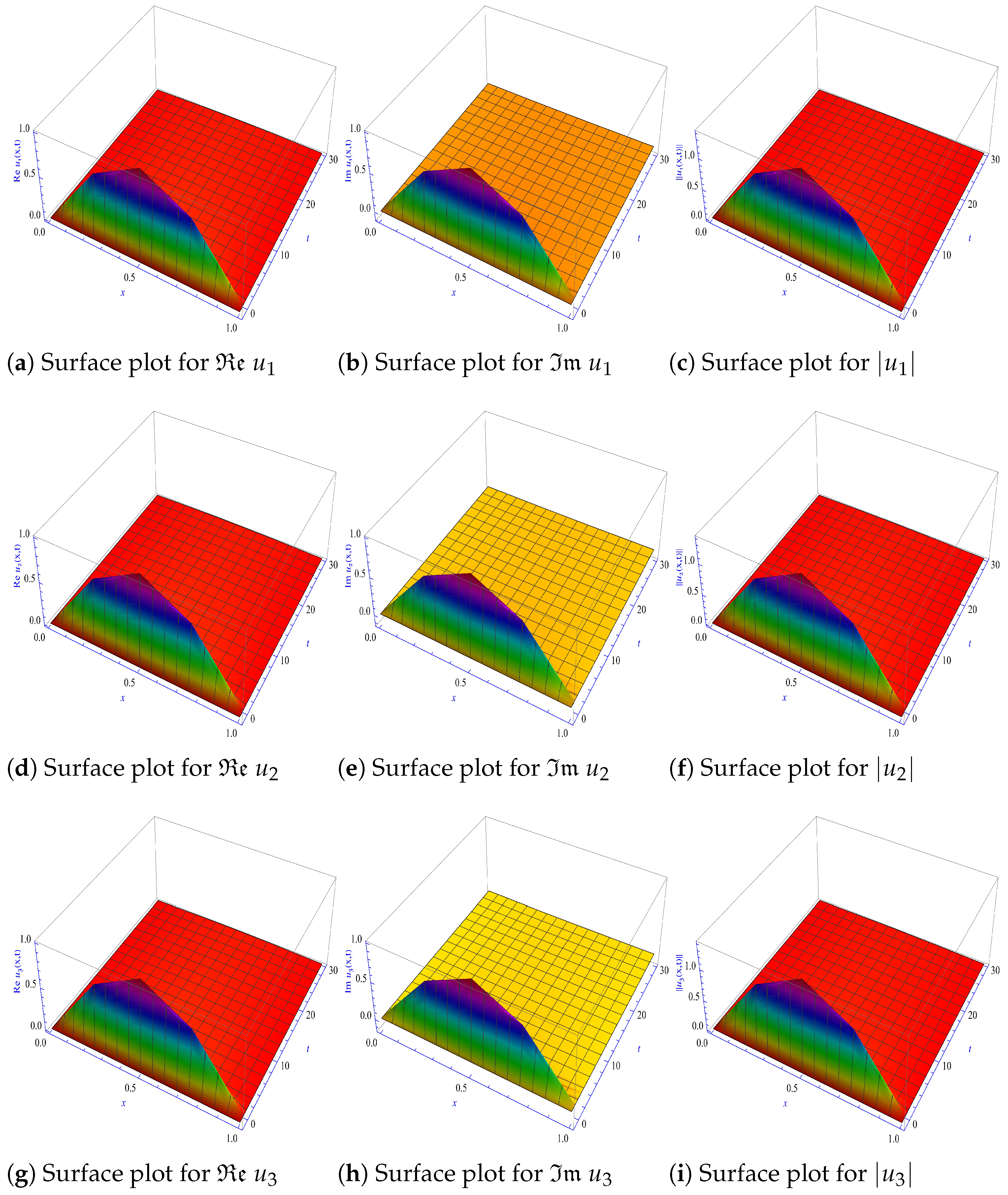
For (${\beta }_1=-4, {\beta }_2=-5, {\beta }_3=-6$) and (${\varrho }_1=1, \varrho =2, {\varrho }_3=3$); in this case, Figure 1 shows that the solutions are asymptotically stable and indicates that the findings are consistent theoretically with Theorem 1 and numerically with Theorems 2 and 3.

(ii) 

For (${\beta }_1=-1, {\beta }_2=-2, {\beta }_3=-3$) and (${\varrho }_1=15, {\varrho }_2=20, {\varrho }_3=25$), with and without delay. It was observed that the delay changes the solution’s behavior from decay (as seen in Figure 2) to non-decay (as shown in Figure 3). This highlights the significant impact of delay on the system’s dynamics.

To verify the temporal convergence, we set mesh size $h=0.1$ and the terminal time $T=1$ with time step size $\tau ={\displaystyle \frac{1}{N_{\tau }}}$. The convergence error in time is defined by ${\mathcal{E}}_{N_{\tau }}^2={\displaystyle \sum _{s=1}^3}{∥u_s^{N_{\tau }}-u_s^{N_{\tau }/2}∥}_{L_2}^2$, and the convergence order is numerically computed by

$$Order={log}_2{\displaystyle \frac{{\mathcal{E}}_{N_{\tau }}}{{\mathcal{E}}_{N_{\tau }/2}}}.$$

Additionally, we present in

Table 1. The $L_2$ norm error for (19) at mesh size $h=0.1$ and terminal time $T=1$ for $\alpha =0.2, 0.6$.

$\mathit{\alpha }$	0.2			0.6
${\mathit{N}}_{\mathbf{\tau }}$	${\mathcal{E}}_{{\mathit{N}}_{\mathbf{\tau }}}$	Order	CPU Time	${\mathcal{E}}_{{\mathit{N}}_{\mathbf{\tau }}}$	Order	CPU Time
$2^5$	$4.84082\times {10}^{-5}$	$1.04488$	$8.031$	$7.93595\times {10}^{-5}$	$1.05114$	$9.875$
$2^6$	$2.34627\times {10}^{-5}$	$1.0224$	$17.921$	$3.82979\times {10}^{-5}$	$1.03064$	$20.5$
$2^7$	$1.15506\times {10}^{-5}$	$1.0112$	$40.046$	$1.87466\times {10}^{-5}$	$1.01716$	$43.703$
$2^8$	$5.73065\times {10}^{-6}$	−	$96.218$	$9.26247\times {10}^{-6}$	−	$100.61$

, the $L_2$ norm error for the numerical solutions, order of convergence for the proposed scheme and CPU time in second for various values of α when (${\beta }_1=-2, {\beta }_2=-3, {\beta }_3=-4$), (${\varrho }_1=1, \varrho =2, {\varrho }_3=3$) and ($c_{s1}=0.2, c_{s2}=0.3, c_{s3}=0.4$), for $s=1,2,3$ in order to show the efficiency of the proposed scheme. Thus, Table 1 indicates that the present scheme achieves an $\mathcal{O}\left(\tau \right)$ order in the sense of $L_2$ norm.

Example 2.

In this example, we consider the system of time-fractional NSDEs

$$\left\{\begin{array}{cc}\hfill {}_0{}^C\mathbf{D}_t^{\alpha }{u}_1=& \mathbf{i}∆u_1+{\beta }_1{u}_1-\left(0.7|u_1{|}^2+0.8|u_2{|}^2+0.9{|u_3|}^2\right)u_1+{\varrho }_1{\tilde{u}}_1,\hfill \\ \hfill {}_0{}^C\mathbf{D}_t^{\alpha }{u}_2=& \mathbf{i}∆u_2+{\beta }_2{u}_2-\left(0.8|u_1{|}^2+0.7|u_2{|}^2+0.9{|u_3|}^2\right)u_2+{\varrho }_2{\tilde{u}}_2,\hfill \\ \hfill {}_0{}^C\mathbf{D}_t^{\alpha }{u}_3=& \mathbf{i}∆u_3+{\beta }_3{u}_3-\left(0.8|u_1{|}^2+0.9|u_2{|}^2+0.7{|u_3|}^2\right)u_3+{\varrho }_3{\tilde{u}}_3,\hfill \end{array}\right.$$

(20)

with the following conditions

$$\left\{\begin{array}{cc}\hfill & u_s(0,t)=u_s\left(2,t\right)=0,fors=1,2,3,t>0.\hfill \\ \hfill & u_s(x,t)=\left(t+2\right)x(2-x)(1+\mathbf{i})for\zeta =2,t\in [-2,0],x\in \left[0,2\right].\hfill \end{array}\right.$$

For this example, at $h=∆t=0.05$ and $n=400$, we analyze the numerical solutions behavior for varying values of $\alpha =0.25, 0.5, 0.75$ in two cases:

(i) 

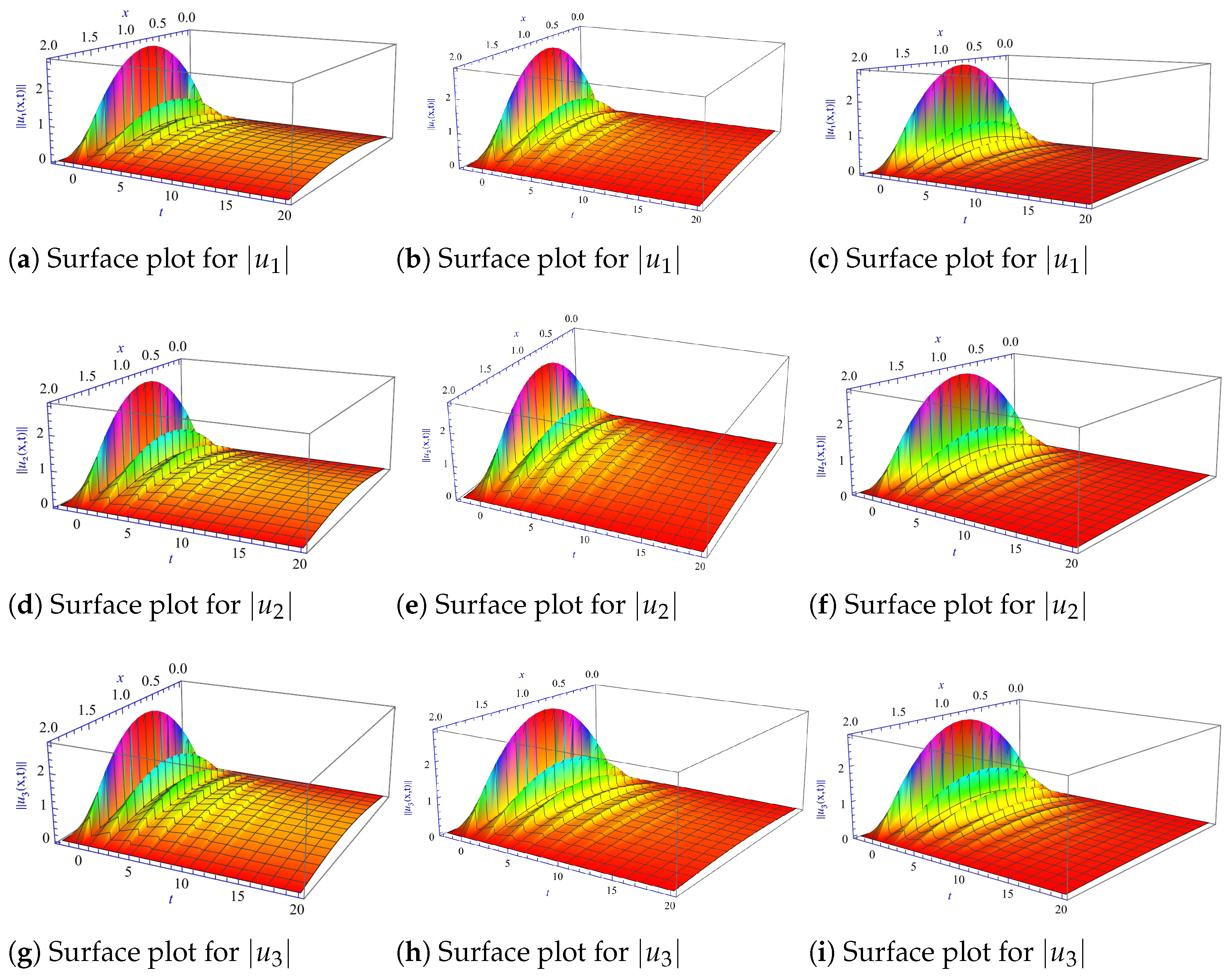
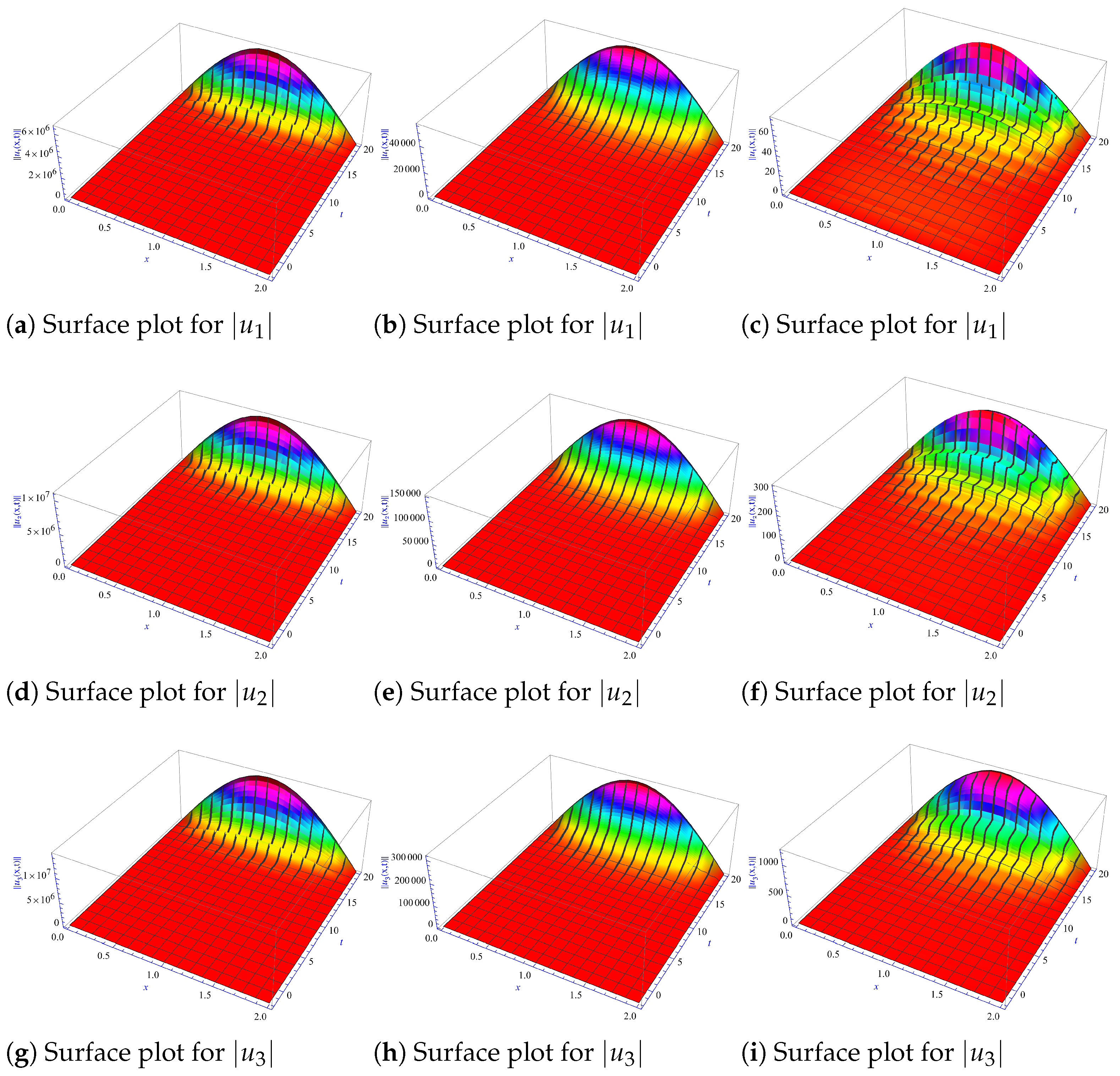
(${\beta }_1=-7, {\beta }_2=-8, {\beta }_3=-9$) and (${\varrho }_1=4, \varrho =5, {\varrho }_3=6$). In Figure 4, many patterns show that the solutions are asymptotically stable and have the same layout for all values of α and investigate that the results are in accordance theoretically with Theorem 1 and numerically with Theorems 2 and 3.

(ii) 

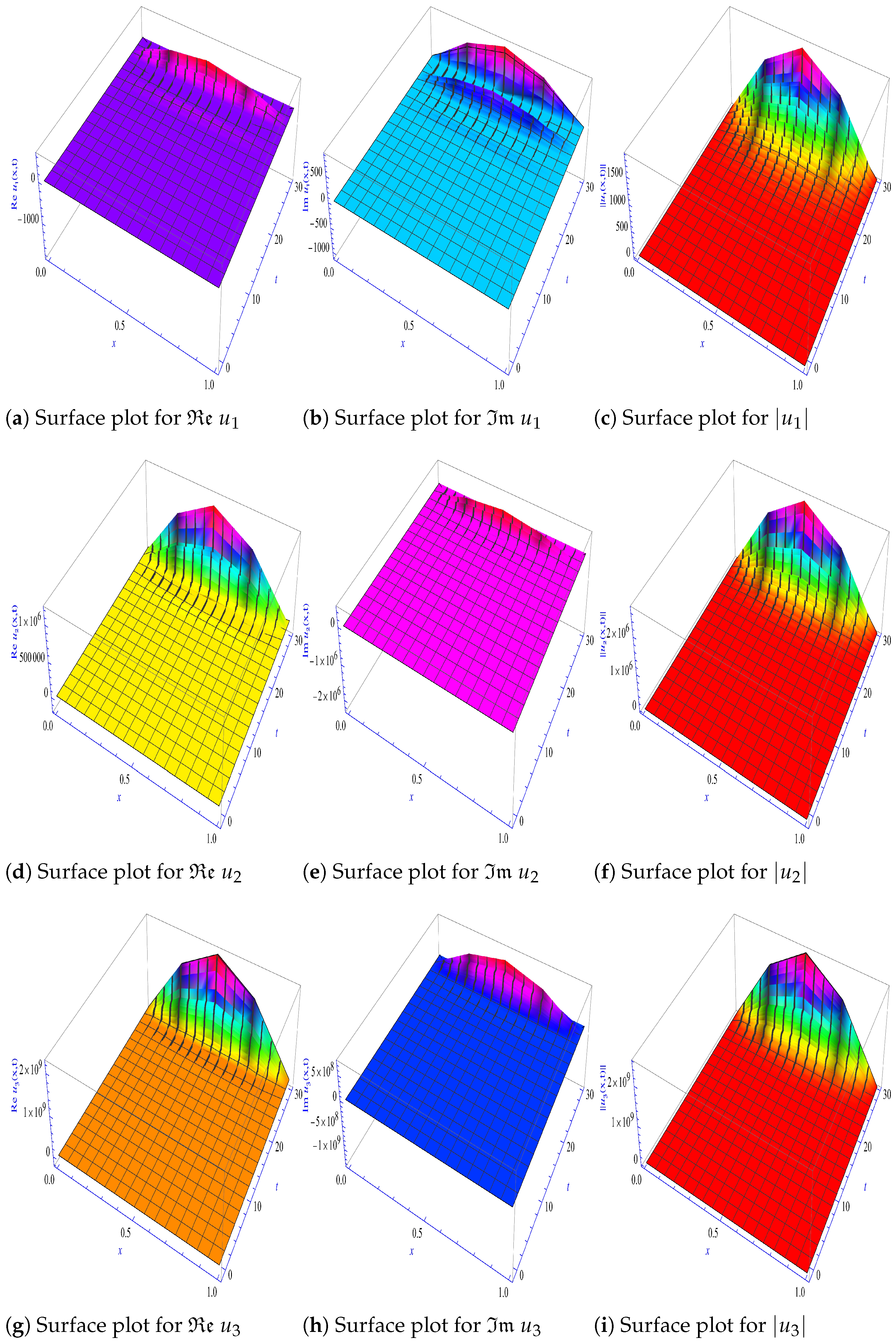
(${\beta }_1=-2, {\beta }_2=-3, {\beta }_3=-4$) and (${\varrho }_1=20, \varrho =25, {\varrho }_3=30$). The results, as shown in Figure 5, demonstrate that the solutions are unstable and also display consistent behavior for all values of α, but it seems that decreasing α makes the solution unstable energetically. These findings investigate that the fractional order α has a significant impact on the qualitative nature of the unstable solutions.

Remark 4.

1.

In Example 1, we illustrate the behavior of the numerical solutions under two scenarios: (i) When hypothesis H1 is satisfied, the solutions demonstrate asymptotic stability, aligning with the theoretical predictions.(ii) When hypothesis H1 is not satisfied, we analyze the solution behavior in two distinct cases: without delay and with delay. The results reveal that the presence of delay significantly influences the long-time stability of the solutions. These findings are in complete agreement with the theoretical results established in Theorem 1 and are further validated numerically through Theorems 2 and 3. The strong correspondence between the theoretical and numerical results investigates the critical role of delay in studying the stability properties of the system.

2.

These findings highlight the significant influence of the fractional order α on the qualitative behavior of the solutions. Specifically, when the solutions exhibit instability, it is evident that decreasing α leads to an energetically unstable solution, as clearly illustrated in the patterns shown in Figure 5.

6. Conclusions

In the context of the Caputo fractional derivative, this study examined the theoretical asymptotic stability and long-time decay of the zero solution for a system of time-fractional NSDEs. We used an energy function in the sense of the $L_2$ norm to theoretically illustrate when the considered system decays and behaves asymptotically via the fractional Halanay inequality. Along with spatial discretization for the space variables by implementing the finite difference approach, we examined the long-time stability for the semi-discrete system. Additionally, we used the L1 technique to approximate the Caputo fractional derivative and examined the long-time stability of the fully discrete system through the system’s discrete energy. Also, it was demonstrated that the numerical technique might accurately reflect the long-time behavior of the considered problem. Lastly, these findings were confirmed by numerical examples. For Higher-order Caputo fractional integro-differential inclusions of Volterra–Fredholm type with impulses and infinite delay: existence results, thorough analysis will be investigated in the future work.

References

- Berezin, F.A.; Shubin, M. The Schrödinger Equation; Springer Science & Business Media: Berlin/Heidelberg, Germany, 2012; Volume 66. [Google Scholar]
- Fibich, G. The Nonlinear Schrödinger Equation; Springer: Berlin/Heidelberg, Germany, 2015; Volume 192. [Google Scholar]
- Khan, N.A.; Hameed, T. An implementation of Haar wavelet based method for numerical treatment of time-fractional Schrödinger and coupled Schrödinger systems. IEEE/CAA J. Autom. Sin. 2016, 6, 177–187. [Google Scholar] [CrossRef]
- Okposo, N.I.; Veeresha, P.; Okposo, E.N. Solutions for time-fractional coupled nonlinear Schrödinger equations arising in optical solitons. Chin. J. Phys. 2022, 77, 965–984. [Google Scholar] [CrossRef]
- Ali, K.K.; Maneea, M. Optical solitons using optimal homotopy analysis method for time-fractional (1+1)-dimensional coupled nonlinear Schrödinger equations. Optik 2023, 283, 170907. [Google Scholar] [CrossRef]
- Ameen, I.G.; Taie, R.O.A.; Ali, H.M. Two effective methods for solving nonlinear coupled time-fractional Schrödinger equations. Alex. Eng. J. 2023, 70, 331–347. [Google Scholar] [CrossRef]
- Zaky, M.A.; Hendy, A.S.; Aldraiweesh, A.A. Numerical algorithm for the coupled system of nonlinear variable-order time fractional Schrödinger equations. Rom. Rep. Phys. 2023, 75, 106. [Google Scholar]
- Hadhoud, A.R.; Agarwal, P.; Rageh, A.A.M. Numerical treatments of the nonlinear coupled time-fractional Schrödinger equations. Math. Methods Appl. Sci. 2022, 45, 7119–7143. [Google Scholar] [CrossRef]
- Onder, I.; Secer, A.; Bayram, M. Optical soliton solutions of time-fractional coupled nonlinear Schrödinger system via Kudryashov-based methods. Optik 2023, 272, 170362. [Google Scholar] [CrossRef]
- Mubashir Hayat, A.; Abbas, M.; Emadifar, H.; Alzaidi, A.S.M.; Nazir, T.; Aini, A.F. An efficient computational scheme for solving coupled time-fractional Schrödinger equation via cubic B-spline functions. PLoS ONE 2024, 19, e0296909. [Google Scholar] [CrossRef] [PubMed]
- Ahmad, J.; Rani, S.; Turki, N.B.; Shah, N.A. Novel resonant multi-soliton solutions of time fractional coupled nonlinear Schrödinger equation in optical fiber via an analytical method. Results Phys. 2023, 52, 106761. [Google Scholar] [CrossRef]
- Wang, Y.; Mei, L. A conservative spectral Galerkin method for the coupled nonlinear space-fractional Schrödinger equations. Int. J. Comput. Math. 2019, 96, 2387–2410. [Google Scholar] [CrossRef]
- Almushaira, M.; Liu, F. Fourth-order time-stepping compact finite difference method for multi-dimensional space-fractional coupled nonlinear Schrödinger equations. SN Partial. Differ. Equ. Appl. 2020, 1, 45. [Google Scholar] [CrossRef]
- Zhao, X.; Yang, Y.; Li, H.; Fang, Z.; Liu, Y. Numerical analysis and computation of the finite volume element method for the nonlinear coupled time-fractional Schrödinger equations. Fractal Fract. 2024, 8, 480. [Google Scholar] [CrossRef]
- Chen, Y.; Guo, J. Unconditional error analysis of the linearized transformed L1 virtual element method for nonlinear coupled time-fractional Schrödinger equation. J. Comput. Appl. Math. 2025, 457, 116283. [Google Scholar] [CrossRef]
- Fridman, E. Introduction to Time-Delay Systems: Analysis and Control; Springer: Cham, Switzerland, 2014. [Google Scholar]
- Gao, Y.; Kostyukova, O.; Chong, K.T. Worst-case optimal control for an electrical drive system with time-delay. Asian J. Control 2009, 11, 386–395. [Google Scholar] [CrossRef]
- Shao, C.; Sheng, J. The framework for linear periodic time-delay systems based on semi-discretization: Stability analysis and control. Asian J. Control 2014, 16, 1350–1360. [Google Scholar] [CrossRef]
- Gumowski, I.; Mira, C.; Pearson, A.E. Optimization in Control Theory and Practice. J. Appl. Mech. Jun 1969, 36, 383. [Google Scholar] [CrossRef]
- Yang, K.Y.; Wang, J.M. Pointwise stabilisation of a string with time delay in the observation. Int. J. Control 2017, 90, 2394–2405. [Google Scholar] [CrossRef]
- Datko, R.; Lagnese, J.; Polis, M. An example on the effect of time delays in boundary feedback stabilization of wave equations. SIAM J. Control Optim. 1986, 24, 152–156. [Google Scholar] [CrossRef]
- Datko, R. Two examples of ill-posedness with respect to time delays revisited. IEEE Trans. Autom. Control 1997, 42, 511–515. [Google Scholar] [CrossRef]
- Tang, S.; Xie, C. State and output feedback boundary control for a coupled PDE–ODE system. Syst. Control Lett. 2011, 60, 540–545. [Google Scholar] [CrossRef]
- Wang, J.M.; Guo, B.Z.; Krstic, M. Wave equation stabilization by delays equal to even multiples of the wave propagation time. SIAM J. Control Optim. 2011, 49, 517–554. [Google Scholar] [CrossRef]
- Guo, B.Z.; Xu, C.Z.; Hammouri, H. Output feedback stabilization of a one–dimensional wave equation with an arbitrary time delay in boundary observation. ESAIM Control. Optim. Calc. Var. 2012, 18, 22–35. [Google Scholar] [CrossRef]
- Čermák, J.; Došlá, Z.; Kisela, T. Fractional differential equations with a constant delay: Stability and asymptotics of solutions. Appl. Math. Comput. 2017, 298, 336–350. [Google Scholar] [CrossRef]
- Wang, H.; Yu, Y.; Wen, G.; Zhang, S.; Yu, J. Global stability analysis of fractional-order Hopfield neural networks with time delay. Neurocomputing 2015, 154, 15–23. [Google Scholar] [CrossRef]
- Xu, Y.; Li, Y.; Li, W. Graph-theoretic approach to synchronization of fractional-order coupled systems with time-varying delays via periodically intermittent control. Chaos Solitons Fractals 2019, 121, 108–118. [Google Scholar] [CrossRef]
- Čermák, J.; Nechvátal, L. On exact and discretized stability of a linear fractional delay differential equation. Appl. Math. Lett. 2020, 105, 106296. [Google Scholar] [CrossRef]
- Li, D.; Zhang, C. Long time numerical behaviors of fractional pantograph equations. Math. Comput. Simul. 2020, 172, 244–257. [Google Scholar] [CrossRef]
- Wang, D.; Xiao, A.; Liu, H. Dissipativity and stability analysis for fractional functional differential equations. Fract. Calc. Appl. Anal. 2015, 18, 1399–1422. [Google Scholar] [CrossRef]
- Wang, D.; Zou, J. Dissipativity and contractivity analysis for fractional functional differential equations and their numerical approximations. SIAM J. Numer. Anal. 2019, 57, 1445–1470. [Google Scholar] [CrossRef]
- Wang, D.; Xiao, A.; Sun, S. Asymptotic behavior of solutions to time fractional neutral functional differential equations. J. Comput. Appl. Math. 2021, 382, 113086. [Google Scholar] [CrossRef]
- Nicaise, S.; Rebiai, S.E. Stabilization of the Schrödinger equation with a delay term in boundary feedback or internal feedback. Port. Math. 2011, 68, 19–39. [Google Scholar] [CrossRef] [PubMed]
- Agirseven, D. On the stability of the Schrödinger equation with time delay. Filomat 2018, 32, 759–766. [Google Scholar] [CrossRef]
- Yao, Z.; Yang, Z. Numerical stability analysis of spatial-temporal fully discrete scheme for time-fractional delay Schrödinger equations. Numer. Algorithms 2024, 97, 1237–1265. [Google Scholar] [CrossRef]
- Zhao, Z.; Ge, W. Traveling wave solutions for Schrödinger equation with distributed delay. Appl. Math. Model. 2011, 35, 675–687. [Google Scholar] [CrossRef]
- Yao, Z.; Yang, Z.; Cheng, L. On the stability preserving of L1 scheme to nonlinear time-fractional Schrödinger delay equations. Math. Comput. Simul. 2025, 231, 209–220. [Google Scholar] [CrossRef]
- Nady, A.; Mathkoor, F.H.; Harun, S.W. Theoretical study on passively mode-locked fiber lasers with saturable absorber. Fiber Integr. Opt. 2019, 38, 76–89. [Google Scholar] [CrossRef]
- Wadati, M.; Iizuka, T.; Hisakado, M. A coupled nonlinear Schrödinger equation and optical solitons. J. Phys. Soc. Jpn. 1992, 61, 2241–2245. [Google Scholar] [CrossRef]
- Rahby, A.S.; Yang, Z. Asymptotic analysis for time fractional FitzHugh-Nagumo equations. J. Appl. Math. Comput. 2025, 71, 3509–3532. [Google Scholar] [CrossRef]
- Podlubny, I. Fractional Differential Equations; Academic Press: San Diego, CA, USA, 1999. [Google Scholar]
- Alikhanov, A. A Priori Estimates for Solutions of Boundary Value Problems for Fractional-Order Equations. Differ. Equ. 2010, 46, 660–666. [Google Scholar] [CrossRef]
- He, B.B.; Zhou, H.C.; Kou, C.H.; Chen, Y. New integral inequalities and asymptotic stability of fractional-order systems with unbounded time delay. Nonlinear Dyn. 2018, 94, 1523–1534. [Google Scholar] [CrossRef]
- Duo, S.; Ju, L.; Zhang, Y. A fast algorithm for solving the space-time fractional diffusion equation. Comput. Math. Appl. 2018, 75, 1929–1941. [Google Scholar] [CrossRef]
- Aksoy, N.Y. On the Convergence of Finite Difference Scheme for a Schrödinger Type Equation. New Trends Math. Sci. 2022, 10, 32–46. [Google Scholar]
- Wang, S.; Nissen, A.; Kreiss, G. Convergence of Finite Difference Methods for the Wave Equation in Two Space Dimensions. Math. Comput. 2018, 87, 2737–2763. [Google Scholar] [CrossRef]
- Applelby, J.A.D.; Győri, I.; Reynolds, D.W. On exact convergence rates for solutions of linear systems of Volterra difference equations. J. Differ. Equ. Appl. 2006, 12, 1257–1275. [Google Scholar] [CrossRef]
- Sun, Z.; Wu, X. A Fully Discrete Difference Scheme for a Diffusion-Wave System. Appl. Numer. Math. 2006, 56, 193–209. [Google Scholar] [CrossRef]
- Lin, Y.; Xu, C. Finite Difference/Spectral Approximations for the Time-Fractional Diffusion Equation. J. Comput. Phys. 2007, 225, 1533–1552. [Google Scholar] [CrossRef]
- Jin, B.; Lazarov, R.; Zhou, Z. An Analysis of the L1 Scheme for the Subdiffusion Equation with Nonsmooth Data. IMA J. Numer. Anal. 2016, 36, 197–221. [Google Scholar] [CrossRef]