Article

Research on the Flexible Job Shop Scheduling Problem with Job Priorities Considering Transportation Time and Setup Time

School of Computer Science and Technology, Harbin University of Science and Technology, Harbin 150080, China
*
Author to whom correspondence should be addressed.
Axioms 2025, 14(12), 914; https://doi.org/10.3390/axioms14120914
Submission received: 6 November 2025 / Revised: 7 December 2025 / Accepted: 9 December 2025 / Published: 12 December 2025

Abstract

This paper addresses the flexible job-shop scheduling problem with multiple time factors—namely, transportation time and setup time—as well as job priorities (referred to as FJSP-JPC-TST). An optimization model is established with the objective of minimizing the completion time. Considering the characteristics of the FJSP-JPC-TST, we propose an improved whale optimization algorithm that incorporates multiple strategies. First, a two-layer encoding mechanism based on operations and machines is introduced. To prevent illegal solutions, a priority-based encoding repair mechanism is designed, along with an active scheduling decoding method that fully considers multiple time factors and job priorities. Subsequently, a multi-level sub-population optimization strategy, an adaptive inertia weight, and a cross-population differential evolution strategy are implemented to enhance the optimization efficiency of the algorithm. Finally, extensive simulation experiments demonstrate that the proposed algorithm offers significant advantages and exhibits high reliability in effectively solving such scheduling problems.

1. Introduction

The Flexible Job-shop Scheduling Problem (FJSP), first introduced by Brucker and Schlie in 1990 [1], has attracted significant research attention due to its broad industrial applicability [2,3]. A key characteristic of the FJSP is that each operation can be processed by multiple functionally similar machines, with processing times for the same operation potentially varying across different machines [4,5]. The primary objective is to optimize the utilization of job-shop resources through efficient allocation of limited available equipment [6]. In recent years, growing demand for customized, low-volume, high-variety production has imposed stricter requirements on production scheduling, particularly for complex product structures. In the manufacturing of industrial products with intricate designs, final products are often assembled from various intermediate components, which are organized hierarchically according to the Bill of Materials (BOM). The completion of child jobs imposes strict constraints on the start times of their parent jobs. Thus, the process flow forms a structured tree that captures both the sequential constraints of operations and the hierarchical constraints among jobs.
On the other hand, the job-shop production time not only refers to the processing time but also includes auxiliary times such as setup time and transportation time. In actual production, enterprises often need to face challenges such as a large variety of products, complex process flows, and parallel production of multiple models, resulting in frequent cross-device transportation and machine setup. Ignoring these auxiliary times will significantly reduce the feasibility of the scheduling plan [7]. In specific job-shop environments such as steelmaking and welding, not considering the setup and transportation times may even cause serious quality problems [8]. It is necessary to further incorporate transportation and setup times into the constraint system in job shop scheduling research, considering job priorities, to optimize process route design and equipment resource allocation, thereby achieving overall scheduling optimization for flexible job shops.
Existing scheduling models often address job priority, transportation time, or setup time in isolation, lacking an integrated approach that captures their synergistic effects in real production environments. To the best of our knowledge, this work is the first to investigate these three constraints simultaneously within a unified framework. Aiming to minimize the makespan, we propose the Flexible Job-shop Scheduling Problem with Job Priority Constraints, Transportation Time, and Setup Time (FJSP-JPC-TST). Unlike the traditional FJSP, where jobs are independent, the FJSP-JPC-TST model incorporates hierarchical job dependencies derived from product BOMs, along with non-negligible transportation and setup times. This integrated approach not only enhances the practical relevance of the scheduling model but also increases its complexity, ultimately supporting the generation of more feasible and effective scheduling solutions for complex manufacturing systems.
Since the FJSP has been proven to be a strongly NP-hard problem [9], the FJSP-JPC-TST studied in this paper also belongs to the NP-hard problem, and a meta-heuristic algorithm with excellent performance needs to be designed to solve this problem. Therefore, we propose an Improved Whale Optimization Algorithm (IWOA) to solve it. IWOA balances global exploration and local exploitation through different hunting methods, and further incorporates a multi-level sub-population optimization strategy, an adaptive inertia weight, and a cross-population differential evolution strategy for optimization. To effectively combine the model and the algorithm, a two-vector coding scheme is proposed, and a correction mechanism is designed to meet the job priority constraints. Finally, the accurate mapping of the production scenario is achieved through decoding.
The structure of this work is arranged as follows: The second section systematically expounds the current research status in the relevant field; Section 3 describes in detail the problem definition and mathematical model of the FJSP-JPC-TST problem; Section 4 proposes a solution method based on the improved whale optimization algorithm; Section 5 covers experimental design, parameter configuration and comparative analysis, verifying the performance of the algorithm through experiments. Section 6 summarizes the research results of the entire text and looks forward to future research directions.

2. Related Work

In traditional FJSP, it is assumed that jobs are independent of each other. To address the production scheduling problem of complex assembly products, researchers introduced job priority constraints into the machining-assembly shop. Vilcot and Billaut [10] were the first to study the priority relationship where multiple predecessors are allowed between operations, but only a single successor. Birgin et al. [11] defined such problems as the extended Flexible Job-shop Scheduling Problem (eFJSP) and established a mixed-integer programming model to simultaneously handle job priority constraints and operation sequence constraints. Based on the above model, researchers have been committed to developing efficient heuristic solution methods. Zou et al. [12] designed a crossover operator and a mutation operator based on hierarchical constraints. However, since the encoded solution needs to be decomposed into multiple levels, it leads to extremely complex solutions for actual large-scale problems. Zhu et al. [13] proposed an ant colony algorithm combined with simulation and the Neo4j semantic graph method to handle FJSP with priority constraints. However, the frequent modification of graphical data in the Neo4j database significantly reduces the computational efficiency. Zhu and Zhou [14] adopted a three-vector encoding combined with a binary sorting tree priority correction mechanism and designed a discrete gray wolf algorithm embedded with a cellular structure to solve the problem. Gao et al. [15] proposed an improved genetic algorithm. The algorithm designed a new genetic operator to ensure the legality of the encoding and enhanced the optimization ability based on local search of machines. Xie et al. [16] proposed an improved artificial bee colony algorithm. The algorithm introduced the evaluation of machining structure and adopted strategies such as dynamic perturbation step size, double-chain similarity, and migration time factor to optimize the scheduling scheme. Lei et al. [17] proposed an improved genetic algorithm based on an operation relationship matrix table. The algorithm designed an encoding based on a dynamic relationship matrix to ensure sequence constraints, designed new crossover and mutation operators to ensure feasibility, and developed a matrix table decoding method. Zhu et al. [18] proposed a shuffling cell evolutionary gray wolf optimizer, which handles job priority constraints through three-vector coding and binary sort tree repair mechanisms, and achieves parallel optimization by leveraging the cell neighborhood structure. With the in-depth research, more complex scenarios have been taken into consideration. Zhu et al. [14] proposed an optimization algorithm based on the leadership hierarchy of multi-micro groups for the FJSP-JPC problem with interval gray processing time. This algorithm implements dynamic decision-making for machine allocation and the construction of uncertain gray scheduling schemes by establishing a multi-micro-group leadership hierarchy, dividing multiple independent micro-group systems for parallel search, and designing bidirectional quantitative encoding and heuristic active gray decoding methods. Li et al. [19] proposed a hybrid adaptive differential evolution algorithm for the FJSP-JPC problem that considers outsourcing strategies, aiming to minimize the number of work-weighted overdue days under different priority weights. By introducing a constraint processing mechanism, the satisfaction of outsourcing conditions is ensured.
However, the above-mentioned research, while accounting for job priority constraints, failed to fully consider the synergistic impact of job transportation time and machine setup time on scheduling decisions. In actual production and manufacturing, time-consuming auxiliary links, such as transportation and setup time, are key factors that cannot be ignored. Even though the auxiliary time is often shorter than the processing time, the machine may not be able to start actual processing due to waiting for the job to arrive and the machine to be ready, which affects the efficiency and smoothness of the overall production plan [20,21].
In the job-shop scheduling considering transportation time, Zhang et al. [20] proposed an improved memetic algorithm, constructed an elite library and distinguished the treatment of solutions, performed simulated annealing on the general solutions to improve the quality, and applied mutation to the local optimal solutions to enhance diversity. Jiang et al. [22] considered both transportation time and deteriorating processes and designed an improved animal migration optimization algorithm to solve it. Pal et al. [23] proposed a decentralized scheduling based on a multi-agent system, which dynamically allocates machine resources through an auction mechanism. The scheduling agent optimizes the operation sequence by combining Gray Wolf Optimization with critical path-based neighborhood search. Chen et al. [24] proposed a cooperative co-evolutionary algorithm based on genetic programming, using hyper-heuristics to generate scheduling rules and combining with adaptive local search. He et al. [25] considered dynamic events arising from uncertainties in industrial production, established a rescheduling model with time compensation based on transportation time, and proposed a Monte Carlo tree search-based algorithm to solve it. In the job-shop scheduling considering setup time, Meng et al. [26] designed three mixed integer linear programming models and a constraint programming model. Li and Lei [27] proposed an imperialist competitive algorithm with feedback. Song et al. [28] proposed a two-stage heuristic algorithm for the distributed assembly permutation flow job-shop scheduling with setup time. Korhan et al. [29] proposed an adaptive evolutionary strategy algorithm for the distributed permutation flow-shop scheduling problem. Chen et al. [30] proposed an evolutionary multitasking optimization framework that adaptively adjusts the knowledge transfer ratio via dynamic migration rates and employs a genetic programming algorithm as a generative hyper-heuristic to handle dynamic uncertainties in the FJSP, considering transportation and setup times.
In summary, research on the FJSP with job priority constraints (JPC) has predominantly focused on JPC alone, with only a few works extending it to scenarios such as outsourcing strategies or fuzzy processing times. On the other hand, studies on FJSP that consider transportation time (T) or setup time (ST) have mostly extended T or ST to contexts like machine deterioration, distributed scheduling, or uncertain environment. However, no existing work has jointly modeled and optimized job priority constraints together with transportation time and setup time. Integrating job priority constraints (JPC), transportation time (T), and setup time (ST) into a unified scheduling framework not only significantly increases the model’s practical relevance but also poses greater challenges to the constraint-handling and search capabilities of solution algorithms. Therefore, we construct the FJSP-JPC-TST model to fill this gap in current research.
As an extension of the FJSP, FJSP-JPC-TST is also NP-hard. Due to the high computational complexity of NP-hard problems, traditional exact algorithms find it difficult to solve them within a reasonable time. Therefore, in recent years, researchers have been committed to developing various meta-heuristic optimization algorithms to effectively handle such problems. These algorithms include genetic algorithm [31,32], particle swarm optimization algorithm [33], ant colony optimization algorithm [34], gray wolf optimization algorithm [35], immune algorithm [36], Harris hawk optimization algorithm [37], memetic algorithm [38], osprey optimization algorithm [39], and sparrow optimization algorithm [40], etc. The Whale Optimization Algorithm (WOA) was proposed by Mirjalili and Lewis [41]. This algorithm simulates the search behavior of whale groups and has the characteristics of simple structure, fast convergence, and strong robustness. It can balance the exploration and exploitation stages of the search space to achieve optimal convergence, and has been practically applied in fields such as feature selection [42], image retrieval [43], robot path planning [44], automatic text summarization [45], and engineering design [46]. As a typical bionic intelligent algorithm, WOA has inherent defects such as being prone to falling into local optima and having a slow convergence speed during the iterative process. For this reason, based on the design of three targeted improvement strategies, we propose an Improved Whale Optimization Algorithm (IWOA) with stronger search ability.

3. Problem Description and Mathematical Model

3.1. Problem Description

In the flexible job shop scheduling scenario, job priorities, transportation time, and setup time need to be clearly defined. Transportation time refers to the time required for a job to transfer between different processing machines; its calculation rule depends on the operation sequence: If the operation is the first operation of a job and the job consists of multiple sub-jobs, the transportation time is the maximum of the times required for each sub-job to independently transfer to the target processing machine. If it is not the first operation, it refers to the time required to transfer the job from the processing machine of the previous operations to the processing machine of the current operations. Setup time refers to the time required for the machine to perform the preparatory work necessary to meet the processing requirements before starting a new processing task. The specific operations include fixture replacement and equipment parameter reset. Optimizing transportation time can significantly reduce non-productive waiting, and optimizing setup time can enhance the production line’s adaptability to multi-variety and small-batch tasks.
The FJSP-JPC-TST model, considering setup time and transportation time, is described as follows. Product P is decomposed into a set J = { J 1 , J 2 , , J n } containing n jobs according to its tree-shaped bill of materials (BOM). Hierarchical constraint relationships are formed among the jobs through the tree-shaped processing technology structure. In the tree structure, the processing of a parent-node job must wait for the completion of all its child-node jobs. It is defined that a child-node job is a predecessor job of the parent-node job, and the parent node is the successor of the child node. Each job J i J contains a set O i = { O i , 1 , O i , 2 , , O i , o i } of o i operations that need to be processed sequentially. Among them, operation O i , j + 1 must start processing only after its predecessor operation O i , j is completed ( j { 1 , 2 , , o i 1 } ). The set of available processing equipment is M = { M 1 , M 2 , , M m } . Each operation O i , j needs to select a machine M k C M i , j from the candidate machine set C M i , j M for processing, and its processing time T i , j , k p r o c depends on the production capacity of the assigned machine. In addition, there are transportation time and setup time during the processing gap of the operation. Machine M k needs a preparation time before processing operation O i , j , denoted as T i , j , k s e t u p . When operation O i , j is completed on machine M k , job J i needs to be transported to the processing machine M q of the next operation via AGV or robot. The fixed transportation time between machines M k and M q is denoted as T R k , q t r a n s . The setup of the machine and the transportation of the job do not interfere with each other and can be carried out simultaneously.
To describe the problem model more specifically, the following assumptions are proposed:
(1)
Each operation can only be processed by one machine, and once processing starts, it must be completed continuously without preemption or interruption allowed.
(2)
Each machine can only process one operation at the same time.
(3)
An operation cannot be interrupted during processing until the operation is completed.
(4)
The processing of a parent job must wait for all its child jobs to be completed.
(5)
There is a sufficient number of AGVs or robots, and all jobs can be immediately transported by any available transportation equipment without AGV competition or waiting time.
(6)
The setup time of an operation on a machine only depends on the machine and the operation and is not affected by other factors.
(7)
Situations such as equipment failures, order insertions, and order cancellations are not considered.
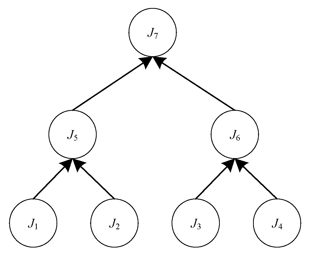
Table 1 and Table 2 and Figure 1 show an example problem instance. The processing operations within each dashed box belong to the same job. Multiple operations of the same job need to be executed in sequence, and the processing sequence among jobs needs to follow the hierarchical constraint relationship based on BOM. Taking job J 5 as an example, the set of predecessor jobs of job J 5 is { J 1 , J 2 } . Assuming that the first operation O 5 , 1 of job J 5 is planned to be processed on machine M 1 , then processing can only start after J 1 completes its last operation O 1 , 3 and J 2 completes its last operation O 2 , 2 , and jobs { J 1 , J 2 } are all transported to machine M 1 , and M 1 also completes the previous processing tasks and the setup time T R 5 , 1 , , 1 s e t u p for operation O 5 , 1 . Table 1 gives the basic processing time and setup time of jobs on machines, separated by “/”, and “-” indicates that this operation cannot be processed on this machine. Table 2 gives the fixed transportation time matrix between machines, with the numbers representing the transportation time.
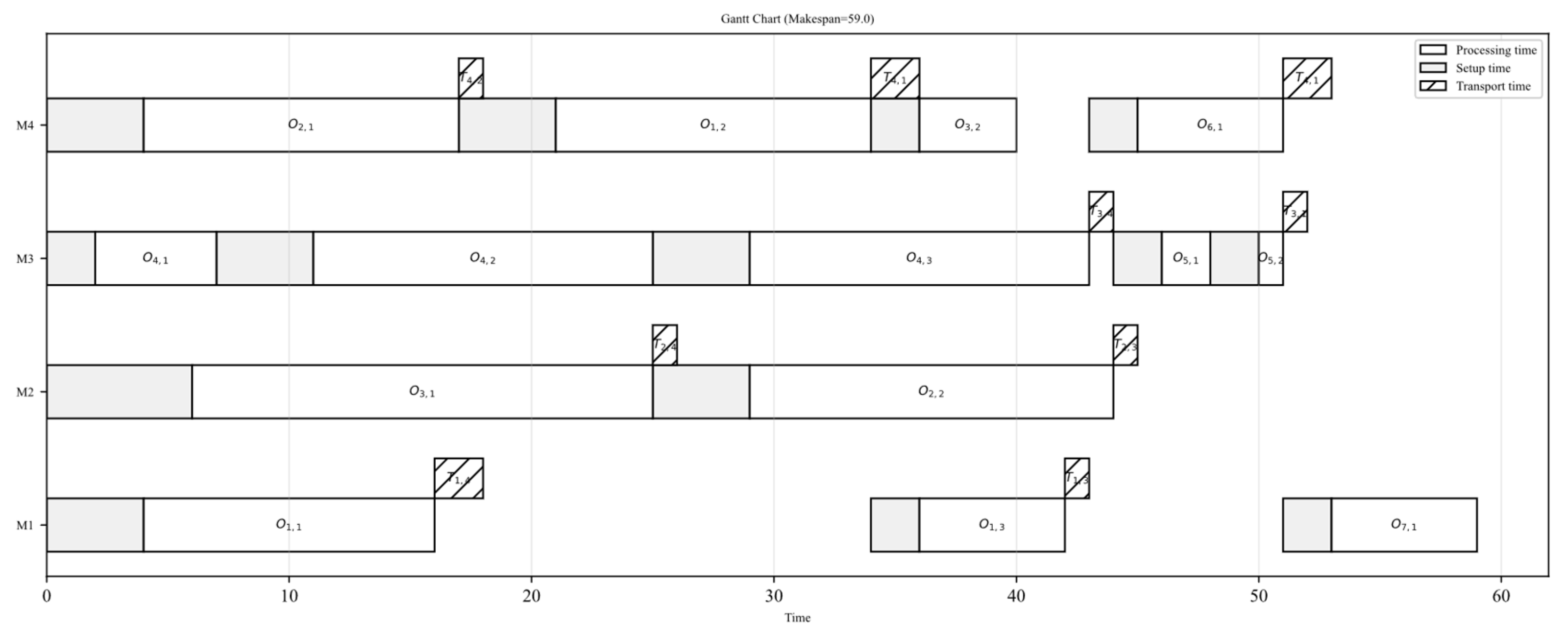
The scheduling scheme Gantt charts of product P are presented in Figure 2. In the figure, processing time is represented by blank bars, with numbers indicating the job and operation numbers. Job transportation time is represented by diagonally striped bars, with numbers identifying destination machine codes. For example, “ T 2 , 1 ” indicates the job is being transported from the current machine M 1 to the target machine M 2 for its next operation. Setup time is represented by gray-shaded bars.

3.2. Mathematical Model

The symbol definitions used in the model are shown in Table 3.
The research problem in this paper is an extension of the classical NP-hard problem. Its core lies in determining the processing sequence to minimize the makespan. The makespan is a key performance indicator for production scheduling problems, ensuring the production cycle and on-time delivery of enterprises. The objective function and related constraints of the FJSP-JPC-TST model in this paper are defined as follows:
The objective aims to minimize the latest completion time among all jobs, i.e., the global makespan. Define the global makespan as C m a x = m a x 1 i n c i . The objective is to minimize C m a x .
f = m i n ( C m a x ) = m i n ( m a x 1 i n c i )
The constraints are grouped into the following categories:
(1)
Non-negativity and variable definitions:
s i , j 0 ,     i = 1 , ,   j n ,   j = 1 , , o i  
c i , j = s i , j + k M T i , j , k p r o c x i , j , k ,     i = 1 , ,   j n , j = 1 , , o i  
c i = c i , J i ,   i = 1 , , j n
(2)
Machine assignment constraints:
k M x i , j , k = 1 ,     i = 1 , , j n   , j = 1 , , o i  
x i , j , k a i , j , k ,     i = 1 , , j n   , j = 1 , , o i   , k M
(3)
Intra-job sequence and transportation constraints:
s i , j c i , j 1 + k M k M T k , k t r a n s z i , j , k , k ,     i = 1 , , j n   , j = 2 , , n i
z i , j , k , k x i , j 1 , k ,     i = 1 , , j n , j = 2 , , o i   , k , k M
z i , j , k , k x i , j , k ,     i = 1 , , j n , j = 2 , , o i   , k , k M
z i , j , k , k x i , j 1 , k + x i , j , k 1 ,     i = 1 , , j n , j = 2 , , o i   , k , k M
(4)
Inter-job precedence (BOM) and transportation constraints:
s i , 1 c i , J i + k M k M T k k t r a n s v i , i , k , k ,     i = 1 , , j n : P i , J i P i
v i , i , k , k x i , J i , k ,     i = 1 , , j n : P i , J i P i , k , k M
v i , i , k , k x i , 1 , k ,     i = 1 , , j n : P i , J i P i , k , k M
v i , i , k , k x i , J i , k + x i , 1 , k 1 ,     i = 1 , , j n : P i , J i P i , k , k M
(5)
Machine processing sequence with setup time constraints:
y i , j , i , j , k + y i , j , i , j , k x i , j , k + x i , j , k 1 ,     k M , ( i , j , i , j ) : ( i , j ) ( i , j )
s i , j c i , j + T i , j , k s e t u p M ( 1 y i , j , i , j , k ) ,     k M , ( i , j , i , j ) : i ( i , j ) ( i , j )
s i , j c i , j + T i , j , k s e t u p M ( 1 y i , j , i , j , k ) ,     k M , ( i , j , i , j ) : ( i , j ) ( i , j )
Equation (2) indicates that the start time of all operations must be non-negative. Equation (3) calculates the end time of each operation. Equation (4) calculates the end time of each job, and the end time of a job is the end time of its last operation. Equation (5) ensures that each operation can only be completed on one machine. Equation (6) ensures that each operation must be processed by its candidate machine. Equation (7) represents the operation sequence constraints (within the same job), which define that the start time of each non-first operation in a job must wait for the completion of the previous operation and add the transportation time. Equations (8)–(10) together ensure that the transportation indicator variable z i , j , k , k equals 1 if and only if operation O i , j 1 is processed on machine M k and operation O i , j is assigned to machine M k . Equation (11) represents the job hierarchy constraints (between jobs), which define that the first operation of the parent job must wait for all child jobs to be completed, and add the transportation time. Equations (12)–(14) activate the transportation variable v i , i , k , k precisely when the last operation of child job J i is finished on machine M k and the first operation of parent job J i is scheduled on machine M k . Equations (15) and (16) define the machine processing sequence constraints, stipulating that for two adjacent operations processed on the same machine, the processing times cannot overlap, and the subsequent operation needs to wait for the previous one to end and add the machine setup time.

4. Solution Method

We propose an improved whale optimization algorithm (IWOA). First, a designed encoding scheme transforms the actual production job-shop scenario into a mathematical representation, and a repair mechanism based on job priorities is designed to ensure feasibility. Second, a hierarchical sub-population collaboration strategy is established to achieve intensive local optimization within sub-populations and enable the migration of high-quality solutions between them. Concurrently, an adaptive inertia weight and a cross-population differential evolution strategy are introduced to enhance the balance between exploration and exploitation, thereby optimizing the population update process. Finally, the solutions are decoded and restored into an executable production scheduling plan.

4.1. Encoding and Decoding

We adopt a two-vector coding scheme, considering job sequencing and machine allocation. To ensure the feasibility of the solution and meet the job priority constraints, a repair mechanism based on job priority is used.

4.1.1. Encoding

A two-vector encoding scheme is adopted. The first layer is the operation sequence vector (OS), which determines the processing order of job operations. Repeated integers represent different operations belonging to the same job. The second layer is the machine selection vector (MS), which identifies the specific machine chosen from the available equipment set for each corresponding operation. Both encoding layers have the same length, equal to the total number of operations, calculated as I = i n o i . Taking the instance of 7 jobs and 4 machines described in Section 3.1 (hereafter referred to as Example 1), the OS vector has a length of 14. As shown in Figure 3, the first element “2” in the OS vector represents operation O 2 , 1 . According to the corresponding element in the MS vector, this operation is assigned to be processed on machine M 2 , selected from its available alternatives. The second element “2” in OS represents operation O 2 , 2 , which is assigned to machine M 1 .
The standard Whale Optimization Algorithm (WOA) is primarily designed for continuous optimization problems. To adapt it for solving discrete scheduling problems, specific conversion rules for both machine encoding and operation encoding are introduced. For machine encoding conversion, the values in the machine position vector are transformed into indices pointing to the candidate machine sets for the corresponding operations, thereby determining the final machine assignments. The conversion is defined by Equation (18).
u ( e ) = round x ( e ) + ϵ 2 ϵ ( s ( e ) 1 ) + 1 , 1 e I
In this context, s ( e ) denotes the number of available machines for the operation corresponding to element e ; x ( e ) represents the value of element e in the machine encoding layer; u ( e ) signifies the index within the candidate machine set assigned to this operation. The element values at individual positions are confined to the interval [ ε , ε ] . Here, ε is a normalization constant. Based on empirical tuning, we set ε = 8 for our experiments. The experiment found that this value provides a sufficient numerical range to stably map continuous values to discrete machine indexes. Correspondingly, when converting a scheduling plan back into machine encoding, the inverse operation of Equation (18) is applied. A numeric example is provided to illustrate the steps. Suppose ε = 8, and for a certain operation, the number of candidate machines is 3, and the continuous value x = −1.5. Then, the machine index is calculated as follows: u   =   r o u n d 1.5 + 8 / 2 × 8 × 3 1 + 1   = 2 . Thus, the second machine in the candidate set is selected.
For operation encoding conversion, the Ranked Order Value (ROV) rule is employed. First, the element values within the operation encoding vector are sorted in ascending order, and corresponding ROVs are assigned to each element. Subsequently, based on the sequence of these ROVs, the operations represented by the elements are ordered to generate an operation sequence, as illustrated in Figure 4. Similarly, the reverse process is adopted when converting a scheduling plan back into operation encoding.
To address the prevalence of infeasible candidate solutions that violate the mixed constraints among randomly generated solutions, we design a correction mechanism based on job priorities to rectify these solutions. First, the original operation sequence (OS) and the given job priority tree, which defines the precedence constraints between jobs, are taken as input. Then, a binary search tree is constructed using the first element in the OS sequence as the root node. For each subsequent element, starting from the root node, a recursive comparison based on priority relationships is performed. If the job corresponding to the current element has a higher priority than the job of the comparison node, the element is inserted into the left subtree; otherwise, it is inserted into the right subtree. This recursive process continues downward until an empty position is found for insertion, causing higher-priority jobs to progressively gather toward the lower-left corner of the tree. Finally, an in-order traversal is performed on the constructed binary search tree, visiting nodes in the order of left subtree, root node, and right subtree, thereby generating a new operation sequence that fully complies with the priority constraints.
The job priority tree for Example 1 is shown in Figure 5. By applying the aforementioned correction mechanism, the solution presented in Figure 5 is adjusted to obtain an encoding scheme that satisfies the mixed constraints, as demonstrated in Figure 6.

4.1.2. Decoding

An active scheduling decoding strategy is adopted. Without violating the mixed priority constraints, the decoding process is not strictly bound by the sequence defined in the operation encoding. Instead, it preferentially selects the arrangement that allows the operation to start processing at the earliest possible time. The specific steps are as follows: Traverse all operations in the OS from left to right. For the current operation O i , j to be scheduled, read the assigned machine M k from the MS encoding and calculate its earliest start time E S T i , j , considering multiple constraints:
(1)
For the non-first operation O i , j ( j 2 ) of any job, its start time E S T i , j must meet the following combined conditions: First, it is necessary to wait for the previous operation O i , j 1 to be completed on machine M p , and add the transportation time T p , k t r a n s of the job from machine M p to the current machine M k ; at the same time, the current machine M k needs to complete the previous processing task and the setup time T i , j , k s e t u p for operation O i , j . Since the transportation process and machine setup can be executed in parallel, the actual value of E S T i , j is determined by the maximum of the transportation ready time and the machine ready time, that is:
E S T i , j = m a x ( c i , j 1 + T p , k t r a n s , F k + T i , j , k s e t u p )
where F k is the completion time of the last operation processed on machine M k .
(2)
For the first operation O i , 1 of any job, if job J i is a parent job, it must additionally wait for the processing and transportation of all its child jobs to be completed, while still satisfying the machine setup constraint as follows:
E S T i , 1 = m a x ( m a x i P i ( c i + T m i , k t r a n s ) ,   F k + T i , 1 , k s e t u p )
where m i is the processing machine of the child job J i . If job J i has no predecessor job, then:
E S T i , 1 = F k + T i , 1 , k s e t u p
Subsequently, select the earliest feasible time interval that can accommodate the operation’s processing time by identifying the earliest idle window on the timeline of machine M k where the current operation can be inserted. Specifically, check each idle period of the machine in chronological order from left to right to determine if it can accommodate the processing time of the current operation. Once a suitable period is found, schedule the operation to start at the beginning of that period and dynamically update the machine’s timeline. If no existing idle window meets the requirement, append the operation to the end of the machine’s task queue. Let the scheduled working time window of machine M k be W k = { ( m s t k , 1 , m e t k , 1 ) , ( m s t k , 2 , m e t k , 2 ) , , ( m s t k , n , m e t k , n ) } , representing the set of already scheduled operations in chronological order. The idle windows can then be derived as F k = { ( 0 , m s t k , 1 ) , ( e t k , 1 , m s t k , 2 ) , , ( m e t k , n , ) } . For each idle window | A , B | , if it satisfies:
A + T i , j , k p r o c B   a n d A E S T i , j
Then, schedule O i , j in this window the actual start time of the operation s i , j = A . If no window satisfies the conditions, append the operation to the end of the machine’s schedule, setting its actual start time s i , j = m a x ( m e t n , E S T i , j ) , then calculate the actual end time of the operation c i , j = A + T i , j , k p r o c , update the working time window of machine M k , and reorder.
W k = W k { ( s i , j , c i , j ) }
Iterate through the above process sequentially and record the start and completion times of each operation. Finally, obtain a complete scheduling plan and use the total production makespan as the fitness value.

4.1.3. Population Initialization

An initial population is generated using a random initialization strategy. For the OS encoding, solutions are initialized randomly. For the MS encoding, three distinct initialization methods are employed with equal probability: (1) randomly selecting a machine from the candidate set; (2) selecting the machine with the shortest processing time for the operation from the candidate set; (3) selecting the machine with the smallest current workload from the candidate set.

4.2. Traditional WOA

The Whale Optimization Algorithm (WOA) simulates the hunting behavior of humpback whales, where initial solutions are iteratively updated to approach the global optimum. The hunting process consists of three main phases: encircling prey, bubble-net attacking, and searching for prey. An adaptive switching strategy governs the transition between these phases.
Encircling Prey: Individuals move towards the current best solution to narrow the encirclement. The position update formulas are:
X i t + 1 = X b e s t t A D 1
D 1 = | C X b e s t t X i t |
A = 2 a r 1 a
C = 2 r 2
a = 2 2 t / T max
Here, X i t + 1 is the position vector of the individual i at the t-th iteration; X b e s t t is the position vector of the individual with the optimal fitness at the t-th iteration; D 1 is the encirclement vector. The parameter a is a linear convergence factor, and its value gradually decreases from 2 to 0 as the number of iterations increases. r 1 and r 2 are random vectors in the [0, 1] interval, and T max is the maximum number of population updates. A and C continuously adjust the change of the whale individual’s position according to the change of a , enabling the current individual to reach different positions around the best whale individual.
Bubble-net Attacking: After encircling the prey, whales perform a spiral bubble-net attack. They move towards the prey along a logarithmic spiral path while the attack radius decays with iterations. The position update formula is:
X i t + 1 = X b e s t t + e b l c o s ( 2 π l ) D 2
D 2 = | X b e s t t X i t |
Here, e b l c o s ( 2 π l ) controls the whale individual to search for the prey in a logarithmic spiral descent manner. The constant b is a constant used to control the spiral shape, usually set to 1. l is a random number in the [0, 1] interval. D 2 is the absolute value of the distance between the current individual and the best individual.
Searching for Prey: To explore new areas, whales randomly select another individual and move towards it. The position update formulas are:
X i t + 1 = X r a n d t A D 3
D 3 = | C X r a n d t X i t |
Here, X r a n d t is a randomly selected whale’s position at iteration t ; D 3 is the random search vector.
Adaptive Switching Strategy: This strategy intelligently balances global exploration and local exploitation through the dynamic parameter A . The absolute value | A | exhibits distinct phase characteristics. In early iterations, a larger a often results in | A | 1 , promoting global exploration. Whales are guided toward a randomly selected individual X r a n d t (Equation (31)), introducing random perturbations that help escape local optima and explore unknown regions, thus maintaining population diversity. As iterations progress and a decays, | A | typically falls below 1, switching to local exploitation. Whales then focus on the current best solution X b e s t t and select with equal probability (50%) either the shrinking encirclement (Equation (24)) or the spiral update path (Equation (29)). This dual mechanism enables fine-grained search near the optimum, using spiral paths to avoid local traps, thereby enhancing convergence accuracy and speed.

4.3. Improved IWOA

4.3.1. Multi-Level Sub-Population Optimization Strategy

In nature, most organisms exist in groups. Individuals with similar habits congregate in specific environments, forming smaller sub-populations. Within each sub-population, individuals share similar living characteristics. The “survival of the fittest” co-evolution is achieved through resource competition within populations, while information exchange occurs between them [47].
Inspired by this ecological mechanism, we establish a hierarchical sub-population collaborative optimization strategy. During initialization, the population is randomly divided into several sub-populations of equal size, each operating as an independent evolutionary unit. Different from traditional methods, we further introduce a hierarchical stratification mechanism. The population is evenly stratified into multiple levels based on fitness values. Each sub-population is then constructed through stratified random sampling to ensure it contains an equal number of individuals from different levels. This approach balances the guidance from elite solutions with the stability of global search. Each sub-population evolves autonomously according to the position update rules of the whale optimization algorithm. This distributed strategy enables different sub-populations to deeply explore distinct regions of the solution space, forming local convergence cores.
To avoid local optima, a recombination mechanism is implemented. After each round of evolution, the quality of the solution set is evaluated based on fitness values. If the optimal solution shows significant improvement, the current structure is maintained. Otherwise, the recombination process is initiated: sub-populations are merged into a complete population, and new sub-populations are reconstructed through stratified random sampling. This facilitates information exchange between sub-populations and helps prevent each sub-population from becoming trapped in local optima during optimization. Geographical overlap may exist between sub-populations, leading to repeated searches of the same region by individuals from different sub-populations during iterations. Although such regional overlap might reduce search efficiency, it can accelerate the location of the global optimum when that optimum lies within the overlapping region. Furthermore, as problem dimensionality increases, overlapping searches in multi-dimensional space contribute to obtaining higher-precision solutions.

4.3.2. Adaptive Inertia Weight

As a key parameter in the Whale Optimization Algorithm (WOA), the inertia weight significantly influences the position update process. The core mechanism of its adaptive adjustment lies in adopting a larger weight during the initial algorithm phase to enhance global exploration capability, and a smaller weight during later iterations to improve local exploitation ability. By adaptively configuring the inertia weight, the algorithm achieves a better balance between exploration and exploitation stages, thereby effectively improving search efficiency and overall performance. Therefore, we design two inertia weight coefficients: the cosine decay inertia weight coefficient w and the exponential inertia weight coefficient v , defined as follows:
w ( t ) = w min + w max w min × 1 + cos ( π × t T ) 2
v ( t ) = w max × w min w max t T k
Here, w max and w min represent the maximum and minimum values of the decaying inertia weight coefficient, respectively, and the decay behavior is governed by the current iteration count t and the maximum iteration number T . The parameter k controls the decay rate of the exponential weight. Finally, the individual position update formulas are modified by incorporating w and v . Table 4 summarizes how w ( t ) and v ( t ) are assigned to each update mode of IWOA, and the corresponding modifications to the position-update formulas are given in Equation (35).
X i t + 1 = w ( t ) X b e s t t A D 1 if   p < 0.5   and   | A | < 1 w ( t ) X b e s t t + e b l c o s ( 2 π l ) D 2 if   p < 0.5   and   | A | 1 v ( t ) X r a n d t A D 3 if   p 0.5

4.3.3. Cross-Population Differential Evolution Strategy

To address the limitation of the Whale Optimization Algorithm (WOA) being prone to local optima, we propose a cross-population differential evolution strategy that integrates the differential evolution (DE) mutation operator with inter-population communication. This strategy operates through two main mechanisms: First, the DE mutation operator is introduced, leveraging the positional differences between the current population’s optimal solution and neighboring individuals to drive the population away from local optima. Second, by incorporating elite solution information from other sub-populations, a gradient-like search direction across sub-populations is constructed, thereby expanding the global exploration scope. Additionally, the random perturbation characteristics of the Gaussian function are utilized to introduce multi-directional disturbances when population stagnation is detected.
In the DE algorithm, the mutation process serves as the core mechanism for population evolution. It achieves a balance between global exploration and local exploitation by applying directional perturbations to each dimension of an individual’s position. We adopt the “DE/current-to-best/1” mutation operator [48], whose formulation is as follows:
X a , c u r r t + 1 = X a , c u r r t + F ( X a , best t X a , c u r r t ) + F ( X a , r 1 t X a , r 2 t ) ,       rand 0 X a , c u r r t + F X a , best t X a , c u r r t + F X b , e l i t e t X b , r 3 t ,       rand > 0
Here, X a , best t , X a , c u r r t , X a , r 1 t , X a , r 2 t represent the position vectors of the best individual, the current individual c u r r being updated, and random individuals r 1 and r 2 from the current sub-population s u b a at iteration t, respectively, with r 1 r 2 c u r r . X b , e l i t e t , X b , r 3 t represent the position vectors of an arbitrarily selected elite individual and a random individual r 3 from another sub-population s u b b at iteration t, respectively. F is a random scaling factor within [0, 0.5], r a n d is a random number uniformly distributed in [0, 1], and p is a predefined probability threshold controlling the operator selection.
The Gaussian function is employed to perturb each dimension of the position vector. The probability density function of the Gaussian distribution is:
N ( x   |   μ , σ 2 ) = 1 σ 2 π exp ( x μ ) 2 2 σ 2
The DE mutant solution X a , c u r r t + 1 after adding a Gaussian perturbation is as follows:
X a , c u r r t + 1 = X a , c u r r t + 1 + N ( 0 , σ 2 ) ( U L )
Here, σ = e λ t / T max is the adaptive standard deviation, λ is a random attenuation coefficient with values between [1, 5], and U L is the solution space scale vector. Since the solution space is normalized to [ ε , ε ] , U L is a constant vector with each component equal to 2 ε . If a component exceeds the interval [ ε , ε ] , after perturbation, a reflection method is used to map it back into the feasible domain. For a value x , the corrected value x is corrected as follows:
x = 2 ε x if   x > ε , 2 ε x if   x < ε , x otherwise .

4.4. Algorithm Steps

Step 1: Parameter Initialization. Set the current number of iterations i t e r = 1 , the maximum number of iterations T _ max , population size N P , number of sub-populations n , and inertia weight coefficients w min and w max . Calculate the sub-population size as N _ s u b = N P / n .
Step 2: Population Initialization and Repair. Generate the initial population using the encoding scheme. Apply the priority constraint repair mechanism to each individual’s Operation Sequence (OS) to ensure compliance with the job hierarchy constraints defined by the Bill of Materials (BOM) tree structure.
Step 3: Fitness Evaluation. Calculate the fitness value for each individual using the active scheduling decoding strategy, where fitness is defined as 1 / C m a x . Record the global best solution and its corresponding fitness value.
Step 4: Hierarchical Sub-population Construction. Sort the entire population in ascending order of fitness and stratify it evenly into four tiers: top 25%, second 25%, third 25%, and bottom 25%. Construct each sub-population through stratified random sampling, ensuring an equal number of individuals are selected from each tier to maintain diversity across solution qualities.
Step 5: Sub-population Evolution. For each whale individual within every sub-population, execute the following steps:
Step 5.1: Update search parameters using adaptive inertia weights.
Step 5.2: Designate the individual with the best fitness as the leader and update positions according to the WOA strategy, followed by priority constraint repair.
Step 5.3: Apply the cross-population differential evolution strategy to the top 20% of elite individuals, followed by priority constraint repair. Replace the original solution if the new solution demonstrates improved fitness.
Step 5.4: Merge the updated sub-population with its previous version, then select the top N _ s u b solutions based on fitness to form the new sub-population.
Step 6: Global Best Solution Update. Compare the best individual from each sub-population against the current global best solution. Update the global best solution if a superior candidate is found.
Step 7: Termination Check. If the i t e r reaches T _ max , terminate the algorithm and output the complete scheduling plan corresponding to the global best solution. Otherwise, i t e r = i t e r + 1 , proceed to Step 8.
Step 8: Population Reorganization. If the global best solution shows improvement in the current iteration, return to Step 5 to continue sub-population evolution. If no improvement occurs, merge all sub-populations into a unified population and return to Step 4 to reconstruct new sub-populations through re-stratification.
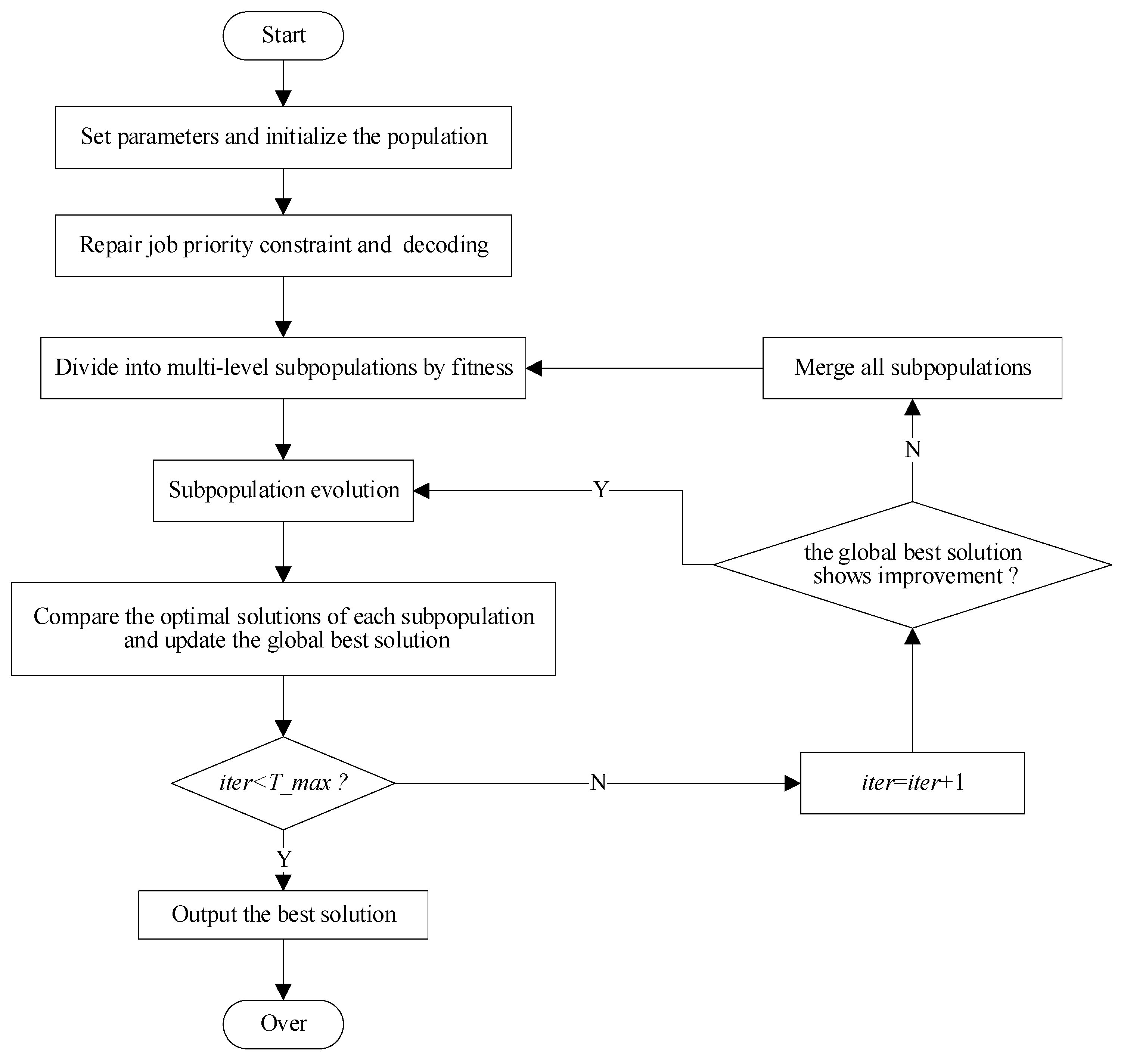
The complete algorithm workflow is illustrated in Figure 7.

4.5. Computational Complexity Analysis

The time complexity per iteration of IWOA is determined by the following key procedures. Initializing the population and applying the priority-based repair mechanism to each individual’s operation sequence collectively require O ( N P I l o g   I ) time. Subsequently, the fitness evaluation, which involves the active scheduling decoder, is performed for each individual. The decoder schedules all I operations sequentially. For each operation, its earliest start time (EST) is computed in O ( 1 ) time. Then, using EST as a lower bound, a binary search is conducted to locate the first possible start position in the sorted timeline of the assigned machine. This search step costs O ( l o g   K ) , where K denotes the current number of scheduled operations on that machine, averaging O ( I / m ) . Following this, a constant number of subsequent idle windows are examined on average until a feasible window is found. Therefore, scheduling a single operation has an average-case time complexity of O ( l o g   ( I / m ) ) , leading to an average decoding complexity of O ( I l o g   ( I / m ) ) per individual. In the worst-case scenario, when all operations are concentrated on a single machine and their EST values are all very small, and the binary search provides limited pruning, potentially raising the cost per operation to O ( I / m ) . Consequently, decoding an individual could reach O ( I 2 / m ) in the worst case. The overall decoding complexity for the population is correspondingly O ( N P I l o g   ( I / m ) ) on average, or O ( N P I 2 / m ) in the worst case. The core position update of the Whale Optimization Algorithm involves arithmetic operations on the 2 I -dimensional encoding vectors, incurring O ( N P I ) time. The cross-population differential evolution strategy also requires vector operations, contributing O ( N P I ) time per iteration. Hierarchical sub-population management, including sorting and reconstruction, is triggered only upon stagnation, with an amortized cost of O ( N P l o g   N P ) per iteration.
Since fitness evaluation is executed in every iteration and dominates the computational cost, the overall average-case time complexity per iteration of IWOA is O ( N P I l o g   ( I / m ) ) , while the worst-case complexity is O ( N P I 2 / m ) .

5. Simulation Experiment Analysis

5.1. Instance Generation

In order to prove the effectiveness of the improved whale algorithm proposed in this paper for solving the FJSP-JPC-TST problem, a large number of experiments were carried out. Due to the lack of a standard benchmark dataset for FJSP-JPC-TST in the open literature, we constructed 12 sets of instance tests that conform to the characteristics of this problem. The rules for generating instances are shown in Table 5. Specifically, the number of jobs ranges from [10, 50], the total number of operations ranges from [30, 210], the number of operations for each job ranges from [1, 5], the number of machines ranges from [4, 9], the job priority depth is set according to the case scale, the processing time follows a discrete uniform distribution in the interval [1, 20], and the transportation time and setup time both follow a discrete uniform distribution in the interval [1, 5]. All the experiments were coded using Python 3.12 and conducted on a computer with an Intel Core i5-12450H@2.80 GHz and 8 GB RAM. In all subsequent experiments, algorithms were independently tested 10 times on each experimental instance.

5.2. Parameter Experiments

The proposed Improved Whale Optimization Algorithm (IWOA) primarily involves four key parameters: the population size N P , the number of subpopulations n , and the non-inertial weight coefficients w min and w max . To determine their optimal values, a Taguchi orthogonal experimental design with four factors and four levels was employed. The parameter levels were set as follows: N P { 100 , 150 , 200 , 250 } , n { 2 , 3 , 4 , 5 } , w min { 0.2 , 0.3 , 0.4 , 0.5 } , w max { 0.6 , 0.7 , 0.8 , 0.9 } . This configuration formed an L 16 ( 4 4 ) orthogonal array, as detailed in Table 6. Using the medium-scale instance T05 as an example, ten independent experiments were conducted for each parameter combination. Each experiment was run for a maximum of 200 iterations. The global optimal solution (i.e., the minimum makespan C _ max obtained in each experiment was recorded, and the mean makespan (denoted as “avg”) across the ten experiments was calculated for each parameter combination. Smaller mean values indicate better performance of the parameter combination. Based on the data in Table 6, the results presented in Figure 8 were obtained. The analysis indicates that the optimal parameter combination is N P = 250 ,   n = 4 ,   w min = 0.3 ,   w max = 0.9 .

5.3. Ablation Experiments

To verify the effectiveness of the proposed improvement strategies, variant algorithms and ablation experiments were designed. IWOA was compared with IWOA1 (IWOA with the Multi-level sub-population optimization strategy removed), IWOA2 (IWOA with the Adaptive Inertia Weight removed), and IWOA3 (IWOA with the Cross-Population Differential Evolution Strategy removed). All algorithms were independently run 10 times, with the minimum (Best) and average (Avg) values of the objective function over multiple runs used as evaluation metrics. Due to the stochastic nature of the algorithms, Wilcoxon rank-sum tests were conducted between IWOA and the variant algorithms at a 95% confidence level. A p-value less than 0.05 indicates a significant difference between the two algorithms. In the ‘win’ column, ‘+’, ‘=’, and ‘−’ indicate that IWOA significantly outperforms, shows no significant difference from, or is significantly worse than the variant algorithm on the corresponding instance, respectively. The last row of the table counts the occurrences of these comparison symbols between IWOA and the compared algorithms, with the results shown in Table 7.
As shown in Table 7, IWOA achieved the smallest Best value in 10 out of 12 instances and the smallest Avg value in 11 instances, demonstrating the effectiveness of the proposed improvement strategies. The Wilcoxon test results show that the comparison outcomes between IWOA and the three variant algorithms are 11/1/0, 10/2/0, and 4/8/0, respectively, indicating that IWOA significantly outperforms the compared algorithms on the vast majority of instances. Specifically, the removal of the Multi-level sub-population optimization strategy has the most significant impact on algorithm performance. This strategy effectively maintains population diversity and avoids premature convergence through hierarchical sampling and a recombination mechanism. The removal of the Adaptive Inertia Weight strategy also leads to significant performance degradation in 10 instances, indicating that this strategy significantly improves the algorithm’s balance between global exploration and local exploitation by dynamically adjusting the search step size. The impact of removing the Cross-Population Differential Evolution Strategy is relatively limited. IWOA significantly outperforms IWOA3 on the four complex instances T07, T09, and T12, while showing no significant difference on the remaining eight instances. This suggests that this strategy primarily serves as an auxiliary enhancement mechanism, providing crucial mutation when the problem structure is complex and local optima traps are deep.

5.4. Comparative Experiments

To validate the performance of the proposed Improved Whale Optimization Algorithm (IWOA), comparative experiments were conducted against other algorithms using extended benchmark instances. Given the limited number of studies specifically addressing the FJSP-JPC-TST problem, we selected FISA_RWPS [15], ABC_MSE [16], ISA_VCLDC [17], MAS_HGWO [23], and the standard WOA, which have been applied to similar scheduling problems, for comparison. To ensure fairness, the population size for all algorithms was uniformly set to 250, and the maximum number of iterations was set to 200.
The remaining parameters were set to their optimal values as reported in the original literature, specifically as follows: In FISA_RWPS, the crossover rate is 0.9 and the mutation rate is 0.3. In ABC_MSE, the search threshold is 30, and the number of scout bees is 3. In ISA_VCLDC, for each small- and medium-scale instance, the crossover rate is 0.9, and the mutation rate is 0.3; for large-scale instances, the crossover rate is 0.6, and the mutation rate is 0.01. The above algorithms are all heuristic algorithms considering job priorities, but do not consider transportation time and setup time. Therefore, the decoding method proposed in this paper is used for adjustment during the decoding stage. In MAS_HGWO, the crossover rate is 0.9. In WOA, parameter α linearly decreases from 2 to 0, the selection probability is a random number in the interval [0, 1], the spiral constant is 1, and a binary tree-based repair mechanism is further used in MAS_HGWO and WOA to ensure job priority constraints. All algorithms were independently run 10 times, and the minimum (Best), average (Avg) of the objective function over multiple runs, and the average CPU running time (Time) of the algorithms are reported, with the results shown in Table 8. Similarly, Wilcoxon rank-sum tests were conducted between IWOA and the comparison algorithms at a 95% confidence level, where a p-value less than 0.05 indicates a significant difference between the two algorithms, and the results are shown in Table 9.
As can be seen from Table 8, IWOA achieved the minimum Best value in 9 out of 12 cases and the minimum Avg value in all instances. The Wilcoxon test results in Table 9 show that the Avg index of the IWOA is not significantly inferior to that of the comparison algorithm in all instances, and it demonstrates a significant advantage in most instances. This indicates that the solutions obtained by IWOA are of higher quality compared to those from the other four algorithms, effectively validating the contribution of the introduced improvement strategies. The superior performance of IWOA can be attributed to several factors: First, the hierarchical sub-population optimization strategy mitigates local search stagnation through collaborative search among stratified sub-populations and a stagnation restart mechanism, thereby enhancing overall convergence performance. Second, the cross-population differential evolution strategy enriches population diversity by applying mutation perturbations to high-quality individuals. Finally, the adaptive inertia weight prioritizes global exploration during the early search stages, and shifts focus to local exploitation in later stages, improving both convergence capability and solution accuracy. In terms of runtime, IWOA demonstrates good scalability. Although its CPU time is higher than that of the standard WOA, it maintains competitive computational efficiency while obtaining better solutions. As the problem scale increases, particularly with the growth in the number of operations, the runtime of IWOA rises accordingly, which primarily stems from the computational burden of fitness evaluation. The largest test instance we used, T12, includes 50 jobs, 220 operations, and 9 machines, which represents a large-scale problem. In this instance, IWOA requires approximately 141.3 s of runtime, whereas the smaller-scale instance T01 needs only 10.3 s. This comparison indicates that although runtime increases significantly with the total number of operations, it remains within an acceptable range. It is worth noting that the parameters of IWOA were optimized through orthogonal experiments under the current testing scale. When the problem scale increases significantly, the optimal parameter configuration may change, and the algorithm may require parameter readjustment. Overall, IWOA achieves an effective balance between computational efficiency and solution quality.
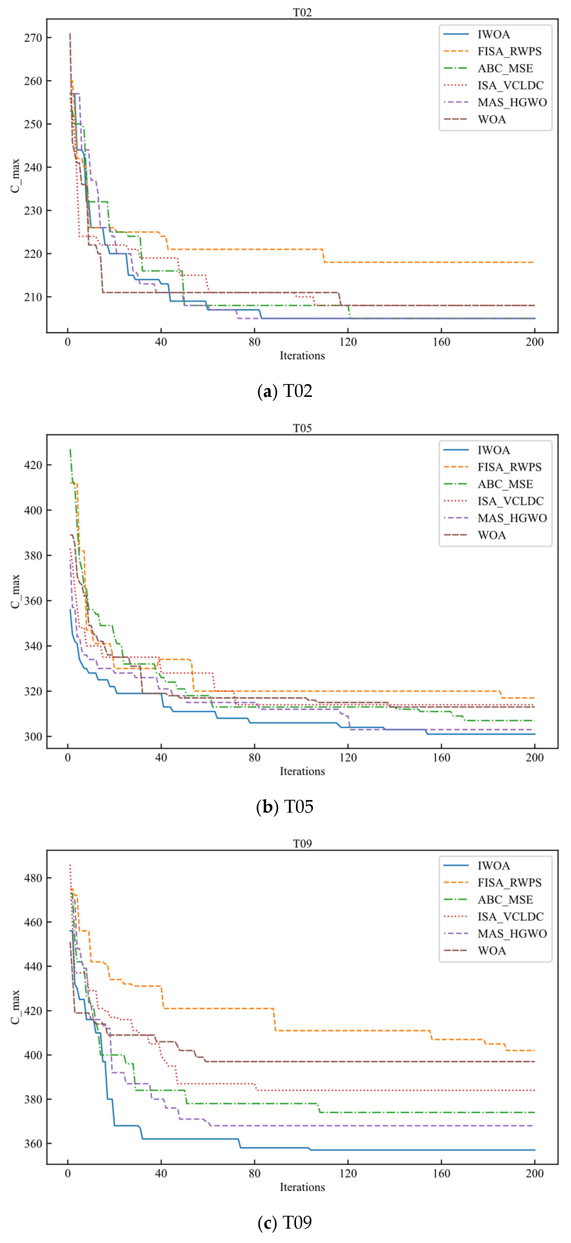
To quantify the stability of the algorithms over multiple runs, we further compared the standard deviation of the results across different algorithms, as shown in Table 10. Table 10 lists the standard deviation of the makespan obtained from 10 independent runs for each compared algorithm on 12 test instances, as well as the performance rank of IWOA in the comparative experiment (denoted by rank, where rank 1 indicates the best performance). The standard deviation directly reflects the fluctuation in solution quality when the algorithm is run multiple times; a smaller standard deviation indicates stronger robustness and repeatability of the algorithm. From Table 10, it can be seen that IWOA achieved the smallest standard deviation in 7 out of the 12 instances, demonstrating optimal stability. For a visual comparison of algorithm performance, representative test instances T02, T05, and T09 were selected for in-depth analysis. Figure 9 presents box plots comparing the results for these three instances. In terms of convergence behavior analysis, Figure 10 displays the convergence curves of the five algorithms on the three test instances. It can be observed that IWOA not only exhibits a faster initial convergence rate but also maintains a continuous improvement trend in the later iterations. The final convergence quality of IWOA is markedly superior to that of the other algorithms. Furthermore, to illustrate the practical scheduling outcomes of IWOA, Figure 11 provides feasible Gantt charts for instances T02, T05, and T09. In summary, when solving the FJSP-JPC-TST problem, compared with the comparison algorithms, the proposed IWOA demonstrates superior performance.

6. Conclusions

This work addresses the flexible job-shop scheduling problem with consideration of multiple time factors and job priorities, and establishes an FJSP-JPC-TST optimization model. To solve this model, we propose an improved whale optimization algorithm (IWOA) incorporating multiple strategies. The algorithm employs a two-layer encoding scheme based on the Ranked Order Value rule, along with an encoding repair mechanism and an active scheduling decoding method, to accommodate scheduling requirements involving multiple time factors and job priorities. Furthermore, a multi-level sub-population optimization strategy is designed to prevent local search stagnation through collaborative search among stratified sub-populations and a stagnation restart mechanism. Additionally, a cross-population differential evolution strategy is introduced to enhance convergence capability and solution accuracy by applying mutation perturbations to high-quality individuals and incorporating adaptive inertia weights. Comparative experimental results demonstrate that IWOA exhibits significant advantages and reliability in solving such scheduling problems.
This research does not account for disruptions caused by dynamic events in actual job-shop production, such as machine failures and order changes, which may affect scheduling plan execution. Meanwhile, the experimental validation in this work is primarily based on simulation instances. Although we have referred to typical characteristics from the industrial scheduling literature when constructing the test cases, conclusions drawn from simulation data still require caution when directly generalizing to specific industrial production scenarios. Therefore, future work will focus on the following aspects: First, a more comprehensive modeling and analysis of dynamic events such as machine failures and urgent order insertions will be conducted to develop more robust scheduling optimization models. More importantly, we will actively seek collaboration with the industrial sector to validate and optimize this method on real manufacturing data platforms, which includes obtaining scheduling logs from actual production environments such as machining centers or assembly lines, so as to further solidify the practicality and application value of the algorithm.

Author Contributions

Conceptualization, C.Z.; Funding acquisition, Z.X.; Methodology, C.Z.; Project administration, C.Z.; Software, Z.X.; Writing—original draft, C.Z.; Writing—Review and Editing, Z.X. and C.Z. All authors have read and agreed to the published version of the manuscript.

Funding

This work was partially supported by the National Natural Science Foundation of China (61772160, Author: Z.X.).

Data Availability Statement

The datasets GENERATED for this work can be found at https://gitee.com/zhengchuchu0807/fjsp-jpc-tst.git (accessed on 6 December 2025).

Conflicts of Interest

The authors declare no conflicts of interest.

Abbreviations

The following abbreviations are used in this manuscript:
FJSPFlexible Job-shop Scheduling Problem
BOMBill of Materials
FJSP-JPC-TSTflexible job-shop scheduling problem with job priority constraints, transportation time, and setup time
IWOAImproved Whale Optimization Algorithm
ROVRanked Order Value

References

  1. Brucker, P.; Schlie, R. Job-shop scheduling with multi-purpose machines. Computing 1990, 45, 369–375. [Google Scholar] [CrossRef]
  2. Gao, K.; Cao, Z.; Zhang, L.; Chen, Z.; Han, Y.; Pan, Q. A review on swarm intelligence and evolutionary algorithms for solving flexible job shop scheduling problems. IEEE/CAA J. Autom. Sin. 2019, 6, 904–916. [Google Scholar] [CrossRef]
  3. Jiang, T.; Liu, L.; Zhu, H.; Li, Y. An Improved Elephant Herding Optimization for Energy-Saving Assembly Job Shop Scheduling Problem with Transportation Times. Axioms 2022, 11, 561. [Google Scholar] [CrossRef]
  4. Liu, L.; Jiang, T.; Zhu, H.; Shang, C. A New Interior Search Algorithm for Energy-Saving Flexible Job Shop Scheduling with Overlapping Operations and Transportation Times. Axioms 2022, 11, 306. [Google Scholar] [CrossRef]
  5. Yin, N.; He, H.; Zhao, Y.; Chang, Y.; Wang, N. Integrating Group Setup Time Deterioration Effects and Job Processing Time Learning Effects with Group Technology in Single-Machine Green Scheduling. Axioms 2025, 14, 480. [Google Scholar] [CrossRef]
  6. Branke, J.; Su, N.; Pickardt, C.W.; Zhang, M. Automated design of production scheduling heuristics: A review. IEEE Trans. Evol. Comput. 2016, 20, 110–124. [Google Scholar] [CrossRef]
  7. Sun, J.; Zhang, G.; Lu, J.; Zhang, W. A hybrid many-objective evolutionary algorithm for flexible job-shop scheduling problem with transportation and setup times. Comput. Oper. Res. 2021, 135, 105263. [Google Scholar] [CrossRef]
  8. Zhang, H.; Xu, G.; Pan, R.; Ge, H. A novel heuristic method for the energy-efficient flexible job-shop scheduling problem with sequence-dependent set-up and transportation time. Eng. Optim. 2022, 54, 1646–1667. [Google Scholar] [CrossRef]
  9. Brandimarte, P. Routing and scheduling in a flexible job shop by tabu search. Ann. Oper. Res. 1993, 41, 157–183. [Google Scholar] [CrossRef]
  10. Vilcot, G.; Billaut, J.C. A tabu search and a genetic algorithm for solving a bicriteria general job shop scheduling problem. Eur. J. Oper. Res. 2008, 190, 398–411. [Google Scholar] [CrossRef]
  11. Birgin, E.G.; Feofiloff, P.; Fernandes, C.G.; de Paula, F.L.; Pedrosa, D.P.; Toffolo, T.A.M. A MILP model for an extended version of the flexible job shop problem. Optim. Lett. 2014, 8, 1417–1431. [Google Scholar] [CrossRef]
  12. Zou, P.; Rajora, M.; Liang, S.Y. A new algorithm based on evolutionary computation for hierarchically coupled constraint optimization: Methodology and application to assembly job-shop scheduling. J. Sched. 2018, 21, 545–563. [Google Scholar] [CrossRef]
  13. Zhu, Z.; Zhou, X.; Shao, K. A novel approach based on Neo4j for multi-constrained flexible job shop scheduling problem. Comput. Ind. Eng. 2019, 130, 671–686. [Google Scholar] [CrossRef]
  14. Zhu, Z.; Zhou, X. Flexible job-shop scheduling problem with job precedence constraints and interval grey processing time. Comput. Ind. Eng. 2020, 148, 106781. [Google Scholar] [CrossRef]
  15. Gao, Y.; Xie, Z.; Yang, D.; Yu, X. Flexible integrated scheduling algorithm based on remaining work probability selection coding. Expert Syst. 2021, 38, e12690. [Google Scholar] [CrossRef]
  16. Xie, Z.; Yang, D.; Ma, M.; Yu, X. An improved artificial bee colony algorithm for the flexible integrated scheduling problem using networked devices collaboration. Int. J. Coop. Inf. Syst. 2020, 29, 2050015. [Google Scholar] [CrossRef]
  17. Lei, Q.; Guo, W.; Song, Y. Integrated scheduling algorithm based on an operation relationship matrix table for tree-structured products. Int. J. Prod. Res. 2018, 56, 5437–5456. [Google Scholar] [CrossRef]
  18. Zhu, Z.; Zhou, X.; Cao, D.; Li, M. A shuffled cellular evolutionary grey wolf optimizer for flexible job shop scheduling problem with tree-structure job precedence constraints. Appl. Soft Comput. 2022, 125, 109235. [Google Scholar] [CrossRef]
  19. Li, H.; Wang, X.; Peng, J. A hybrid differential evolution algorithm for flexible job shop scheduling with outsourcing operations and job priority constraints. Expert Syst. Appl. 2022, 201, 117182. [Google Scholar] [CrossRef]
  20. Zhang, G.; Sun, J.; Lu, X.; Zhang, H. An improved memetic algorithm for the flexible job shop scheduling problem with transportation times. Meas. Control 2020, 53, 1518–1528. [Google Scholar] [CrossRef]
  21. Homayouni, S.M.; Fontes, D.B.M.M. Production and transport scheduling in flexible job shop manufacturing systems. J. Glob. Optim. 2021, 79, 437–465. [Google Scholar] [CrossRef]
  22. Jiang, T.; Zhu, H.; Liu, L.; Gong, Q. Energy-conscious flexible job shop scheduling problem considering transportation time and deterioration effect simultaneously. Sustain. Comput. Inform. Syst. 2022, 35, 100680. [Google Scholar] [CrossRef]
  23. Pal, M.; Mittal, M.L.; Soni, G.; Chouhan, S.S.; Kumar, M. A multi-agent system for FJSP with setup and transportation times. Expert Syst. Appl. 2023, 216, 119474. [Google Scholar] [CrossRef]
  24. Chen, X.; Li, J.; Wang, Z.; Li, J.; Gao, K. A genetic programming based cooperative evolutionary algorithm for flexible job shop with crane transportation and setup times. Appl. Soft Comput. 2025, 169, 111456. [Google Scholar] [CrossRef]
  25. He, Z.; Tang, B.; Gu, C.; Ran, N. Enhanced Monte-Carlo tree search for dynamic flexible job shop scheduling with transportation time constraints. Expert Syst. 2025, 42, e13727. [Google Scholar] [CrossRef]
  26. Meng, L.; Gao, K.; Ren, Y.; Zhang, B.; Sang, H.; Zhang, C. Novel MILP and CP models for distributed hybrid flowshop scheduling problem with sequence-dependent setup times. Swarm Evol. Comput. 2022, 71, 101063. [Google Scholar] [CrossRef]
  27. Li, M.; Lei, D. An imperialist competitive algorithm with feedback for energy-efficient flexible job shop scheduling with transportation and sequence-dependent setup times. Eng. Appl. Artif. Intell. 2021, 103, 104320. [Google Scholar] [CrossRef]
  28. Sun, H.-B.; Chen, Y.-R.; Lin, J. An effective two-stage heuristic for scheduling the distributed assembly flowshops with sequence dependent setup times. Comput. Oper. Res. 2025, 173, 106890. [Google Scholar] [CrossRef]
  29. Karabulut, K.; Ztop, H.; Kizilay, D.; Tasgetiren, M.F.; Kandiller, L. An evolution strategy approach for the distributed permutation flowshop scheduling problem with sequence-dependent setup times. Comput. Oper. Res. 2022, 142, 105733. [Google Scholar] [CrossRef]
  30. Chen, X.; Li, J.; Wang, Z.; Chen, Q.; Gao, K.; Pan, Q. Optimizing Dynamic Flexible Job Shop Scheduling Using an Evolutionary Multi-Task Optimization Framework and Genetic Programming. IEEE Trans. Evol. Comput. 2025, 29, 1502–1516. [Google Scholar] [CrossRef]
  31. Liu, X.; Jiang, D.; Tao, B.; Jiang, G.Z.; Sun, Y.; Kong, J.Y.; Chen, B.J. Genetic algorithm-based trajectory optimization for digital twin robots. Front. Bioeng. Biotechnol. 2021, 9, 793782. [Google Scholar] [CrossRef] [PubMed]
  32. Teng, G. An improved genetic algorithm for dual-resource constrained flexible job shop scheduling problem with tool-switching dependent setup time. Expert Syst. Appl. 2025, 281, 123456. [Google Scholar] [CrossRef]
  33. Kong, J.; Wang, Z. Research on flexible job shop scheduling problem with handling and setup time based on improved discrete particle swarm algorithm. Appl. Sci. 2024, 14, 2586. [Google Scholar] [CrossRef]
  34. Shi, K.J.; Huang, L.; Jiang, D.; Sun, Y.; Tong, X.L.; Xie, Y.M.; Fang, Z.F. Path planning optimization of intelligent vehicle based on improved genetic and ant colony hybrid algorithm. Front. Bioeng. Biotechnol. 2022, 10, 905983. [Google Scholar] [CrossRef]
  35. Jasim, A.M.; Jasim, B.H.; Bures, V. A novel grid-connected microgrid energy management system with optimal sizing using hybrid grey wolf and cuckoo search optimization algorithm. Front. Energy Res. 2022, 10, 960141. [Google Scholar] [CrossRef]
  36. Chen, X.L.; Li, J.Q.; Xu, Y. Q-learning based multi-objective immune algorithm for fuzzy flexible job shop scheduling problem considering dynamic disruptions. Swarm Evol. Comput. 2023, 83, 101398. [Google Scholar] [CrossRef]
  37. Lv, Z.; Zhao, Y.; Kang, H.; Gao, Z.; Qin, Y. An improved Harris hawk optimization algorithm for flexible job shop scheduling problem. Comput. Mater. Contin. 2024, 78, 2337–2360. [Google Scholar] [CrossRef]
  38. Luo, Q.; Deng, Q.; Gong, G.; Guo, X.; Liu, X. A distributed flexible job shop scheduling problem considering worker arrangement using an improved memetic algorithm. Expert Syst. Appl. 2024, 239, 117984. [Google Scholar] [CrossRef]
  39. Dehghani, M.; Trojovský, P. Osprey optimization algorithm: A new bio-inspired metaheuristic algorithm for solving engineering optimization problems. Sci. Rep. 2023, 13, 19583. [Google Scholar] [CrossRef]
  40. Zhang, X.F.; Xiao, F.; Tong, X.L.; Yun, J.T.; Liu, Y.; Sun, Y.; Chen, B.J. Time optimal trajectory planning based on improved sparrow search algorithm. Front. Bioeng. Biotechnol. 2022, 10, 852408. [Google Scholar] [CrossRef]
  41. Mirjalili, S.; Lewis, A. The whale optimization algorithm. Adv. Eng. Softw. 2016, 95, 51–67. [Google Scholar] [CrossRef]
  42. Got, A.; Moussaoui, A.; Zouache, D. Hybrid filter-wrapper feature selection using whale optimization algorithm: A multi-objective approach. Expert Syst. Appl. 2021, 183, 115312. [Google Scholar] [CrossRef]
  43. Aziz, M.A.E.; Ewees, A.A.; Hassanien, A.E. Multi-objective whale optimization algorithm for content-based image retrieval. Multimed. Tools Appl. 2018, 77, 27659–27679. [Google Scholar] [CrossRef]
  44. Tang, R.; Tang, X.; Zhao, H. Enhancing whale optimization algorithm with differential evolution and Lévy flight for robot path planning. Int. J. Adv. Comput. Sci. Appl. 2024, 15, 401. [Google Scholar] [CrossRef]
  45. Gurusamy, B.M.; Rangarajan, P.K.; Altalbe, A. Whale-optimized LSTM networks for enhanced automatic text summarization. Front. Artif. Intell. 2024, 7, 1399168. [Google Scholar] [CrossRef] [PubMed]
  46. Got, A.; Moussaoui, A.; Zouache, D. A guided population archive whale optimization algorithm for solving multiobjective optimization problems. Expert Syst. Appl. 2020, 141, 112972. [Google Scholar] [CrossRef]
  47. Feng, S.; Jia, J. Acceleration sensor placement technique for vibration test in structural health monitoring using microhabitat frog-leaping algorithm. Struct. Health Monit. 2017, 16, 589–602. [Google Scholar] [CrossRef]
  48. Yi, W.; Chen, Y.; Pei, Z.; Lu, J. Adaptive differential evolution with ensembling operators for continuous optimization problems. Swarm Evol. Comput. 2022, 69, 100994. [Google Scholar] [CrossRef]
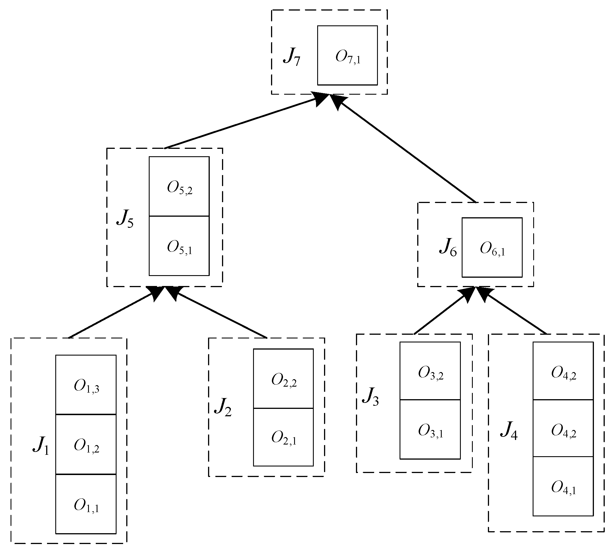
Figure 1. The processing technology tree of Product P (An arrow denotes the precedence constraint between jobs, where the job at the arrow tail must be processed before the job at the arrowhead).
Axioms 14 00914 g001
Figure 2. Gantt chart for the scheduling of Product P (Blank bars represent processing time, diagonally striped bars represent transportation time, and gray-shaded bars represent setup time).
Axioms 14 00914 g002
Figure 3. Example of decoding OS and MS into a scheduling solution (In the OS, the numbers represent Job IDs. Their sequence indicates the processing order of operations. The nth occurrence of the same number represents the nth operation of that job. In the MS, the numbers represent Machine IDs assigned to the corresponding operation. The same applies hereafter).
Axioms 14 00914 g003
Figure 4. Illustration of the ROV rule for OS (Row 2 lists the job IDs for all operations. Each of these IDs is assigned a random value from Row 1. The values are sorted ascendingly to produce the ROV sequence (Row 3), whose order is then mapped back to the job IDs in Row 2 to yield the final operation sequence (Row 4)).
Axioms 14 00914 g004
Figure 5. Job priority tree (defined by the BOM structure; an arrow from a child job points to its parent job, indicating that the job at the tail of the arrow must be processed before the job at the head of the arrow can start).
Axioms 14 00914 g005
Figure 6. A repaired OS encoding after applying the job-priority correction mechanism.
Axioms 14 00914 g006
Figure 7. Flowchart of the proposed IWOA.
Axioms 14 00914 g007
Figure 8. Influence of key algorithm parameters on the average makespan: (a) population size N P , (b) number of subpopulations n , (c) minimum inertia weight w m i n , (d) maximum inertia weight w m a x .
Axioms 14 00914 g008
Figure 9. Box plots for different algorithms for instances (a) T02, (b) T05, and (c) T09 (The horizontal line and the dots within the box represent the median and the mean, respectively).
Axioms 14 00914 g009
Figure 10. Convergence Curves of different algorithms for instances (a) T02, (b) T05, and (c) T09.
Axioms 14 00914 g010
Figure 11. Gantt charts of the optimal schedules generated by the IWOA for instances (a) T02, (b) T05, and (c) T09 (The legends in Figures T05 follow the same convention as established in Figure T02).
Axioms 14 00914 g011aAxioms 14 00914 g011b
Table 1. Data model of Product P .
JobsOperations
M 1
M 2
M 3
M 4
J1O1,112/4---
O1,2-8/22/213/4
O1,36/2-20/6-
J2O2,1-17/59/313/4
O2,2-15/4-20/6
J3O3,1-19/6--
O3,2--20/64/2
J4O4,1--5/216/5
O4,212/4-14/4-
O4,3--14/4-
J5O5,1--2/219/6
O5,2-16/51/2-
J6O6,1-17/5-6/2
J7O7,16/215/4-18/5
Table 2. Transportation Time between Machines.
M 1 M 2 M 3 M 4
M 1 0112
M 2 1011
M 3 1101
M 4 2110
Table 3. Symbol definitions.
Symbol TypeSymbolSymbol Description
Parameter J Set of all jobs
J i The i -th job, i = 1 , 2 , , n
O i , j The j -th operation of job J i , j = 1 , 2 , , o i
M Set of all machines
M k The k -th machine, k = 1 , 2 , , m
P i Set of predecessor jobs of job J i
M A sufficiently large constant
j n Total number of jobs in the product
o i Number of operations in job J i
m n Total number of machines
a i , j , k 1 if machine M k is a candidate machine for operation O i , j , otherwise 0
T i , j , k p r o c Processing time of operation O i , j on machine M k
T i j , k s e t u p Setup time of operation O i , j on machine M k
T k , q t r a n s Transportation time between machines M k and M q
Variable S i , j Start time of operation O i , j
C i , j Completion time of operation O i , j
C i Completion time of job J i
x i , j , k 1 if O i , j is processed on machine M k , otherwise 0
y i , j , i , j , k y i , j , i , j , k = 1 when operation O i , j is processed on machine M k before another operation O i , j , otherwise 0
z i , j , k , k z i , j , k , k = 1 when operation O i , j 1 is processed on machine M k and O i , j is processed on another machine M k , otherwise 0
v i , i , k , k v i , i , k , k = 1 when the last operation of sub-job J i is processed on M k and the first operation of the parent job J i is processed on another machine M k , otherwise 0
Table 4. Inertia Weight Usage in IWOA Update Modes.
Update ModeConditionInertia WeightCorresponding Behavior
Encircling prey p < 0.5   and   | A | < 1 w ( t ) Local exploitation:
shrinking towards the current best
Bubble-net attacking p < 0.5   and   | A | 1 w ( t ) Local exploitation:
spiral search around the best
Searching for prey p 0.5 v ( t ) Global exploration:
moving towards the random individual
Table 5. Instance settings. JN, ON, and MN denote the number of jobs, the total number of operations, and the number of machines, respectively.
InstanceJNONMNInstanceJNONMN
T0110394T07351407
T0215584T08401557
T0320805T09401708
T04251175T10451828
T05301236T11452019
T06301336T12502209
Table 6. Experimental Table of Parameter Combinations.
Number of ExperimentsParameterAvg
N P n W min W m a x
110020.20.6326.8
210030.30.7324.7
310040.40.8322.3
410050.50.9324.8
515020.30.8310.9
615030.20.9312.1
715040.50.6330.2
815050.40.7320.9
920020.40.9318.8
1020030.50.8319.0
1120040.20.7308.7
1220050.30.6322.1
1325020.50.7322.8
1425030.40.6317.3
1525040.30.9306.4
1625050.20.8320.1
Table 7. Results of ablation experiments.
InstanceIWOAIWOA1IWOA2IWOA3
BestAvgBestAvgpWinBestAvgpWinBestAvgpWin
T01145.0145.0145.0145.01.0000=145.0145.01.0000=145.0145.01.0000=
T02205.0207.5208.0210.80.0102+210.9210.00.0091+205.0210.80.0588=
T03199.0204.9206.0209.90.0113+208.4208.00.0821=205.0208.10.0757=
T04292.0296.7303.0306.00.0002+304.8306.00.0004+297.0303.20.0058+
T05301.0304.9306.0309.00.0312+309.8315.00.0211+301.0307.20.1988=
T06306.0313.0317.0324.50.0004+319.3329.00.0041+312.0316.90.1405=
T07318.0328.0330.0341.10.0010+338.8351.00.0032+330.0337.10.0028+
T08347.0358.8361.0373.60.0012+371.6378.00.0022+356.0362.80.2730=
T09354.0363.1388.0402.90.0002+390.4402.00.0002+372.0378.80.0004+
T10341.0347.5358.0365.80.0002+359.7382.00.0009+348.0354.90.0588=
T11326.0338.0342.0351.10.0073+351.5356.00.0025+331.0343.60.1124=
T12483.0495.7514.0523.10.0002+519.0536.00.0002+496.0505.80.0343+
+/=/−11/1/010/2/04/8/0
Table 8. Results of comparative experiments.
InstanceIWOAFISA_RWPSABC_MSEISA-VCLDCMAS_HGWOWOA
BestAvgTimeBestAvgTimeBestAvgTimeBestAvgTimeBestAvgTimeBestAvgTime
T01145.0145.010.3145.0147.112.8145.0145.511.7145.0146.310.7145.0145.213.5 145.0145.910.4
T02205.0207.514.9210.0214.426.6205.0211.023.3208.0212.121.7205.0209.726.8 208.0211.213.5
T03199.0204.922.8208.0213.639.8205.0209.034.9208.0210.330.7199.0205.448.5 206.0210.219.3
T04292.0296.733.9306.0310.373.6297.0301.057.2301.0305.738.8296.0301.876.6 302.0306.031.3
T05301.0304.954.3315.0318.4100.1305.0310.777.9311.0317.057.3303.0308.283.1 310.0315.148.3
T06306.0313.062.3329.0335.7129.2312.0317.885.4316.0327.568.8313.0318.492.7 320.0326.451.9
T07318.0328.077.8349.0362.9159.2327.0340.779.4332.0341.285.9325.0335.1122.5 336.0343.569.8
T08347.0358.8107.1378.0386.7170.5358.0365.9142.7364.0374.5118.3352.0363.8138.7 368.0376.6102.3
T09354.0363.1114.7402.0409.0218.3372.0379.8117.1382.0395.1131.6368.0381.6148.8 396.0404.595.6
T10341.0347.5123.1382.0389.2259.1349.0357.0135.2376.0382.5149.3344.0353.8183.9 393.0399.2122.6
T11326.0338.0129.7356.0376.7277.2339352.2164.8348.0360.5189.1337.0348.8205.4 386.0394.2128.1
T12483.0495.7141.3536.0546.9314.4510.0517.2194.7522.0530.9215.0505.0515.6232.5 546.0558.8137.8
Table 9. The Wilcoxon test results of the comparative experiment.
InstanceFISA_RWPSABC_MSEISA-VCLDCMAS_HGWOWOA
pWinpWinpWinpWinpWin
T010.0588=0.4497=0.0588=1.0000=0.1306=
T020.0012+0.0233+0.0058+0.1405=0.0065+
T030.0012+0.0640=0.0046+0.7055=0.0113+
T040.0002+0.1041=0.0006+0.0312+0.0002+
T050.0002+0.0082+0.0004+0.0696=0.0005+
T060.0002+0.0452+0.0003+0.0173+0.0002+
T070.0002+0.0013+0.0003+0.0091+0.0002+
T080.0002+0.0312+0.0003+0.1620=0.0002+
T090.0002+0.0002+0.0002+0.0007+0.0002+
T100.0002+0.0062+0.0002+0.0376+0.0002+
T110.0002+0.0036+0.0002+0.0156+0.0002+
T120.0002+0.0002+0.0002+0.0002+0.0002+
+/=/−11/1/09/3/011/1/07/5/011/1/0
Table 10. Standard deviation of the comparative experiment.
InstanceIWOAFISA_RWPSABC_MSEISA-VCLDCMAS_HGWOWOARank
T010.02.21.11.50.01.31
T022.63.73.04.13.42.22
T033.74.22.63.23.73.64
T043.94.24.84.04.64.51
T054.04.25.24.74.74.31
T064.35.94.76.94.44.71
T074.86.06.38.75.35.31
T086.47.05.67.57.98.22
T096.25.55.58.811.56.63
T105.46.76.67.17.05.71
T117.69.48.78.67.97.22
T128.29.89.78.59.39.71
Disclaimer/Publisher’s Note: The statements, opinions and data contained in all publications are solely those of the individual author(s) and contributor(s) and not of MDPI and/or the editor(s). MDPI and/or the editor(s) disclaim responsibility for any injury to people or property resulting from any ideas, methods, instructions or products referred to in the content.