
Automatic Frequency Identification under Sample Loss in Sinusoidal Pulse Width Modulation Signals Using an Iterative Autocorrelation Algorithm

 ,
,
Abstract
:
1. Introduction
2. Signal Analysis Background Theory
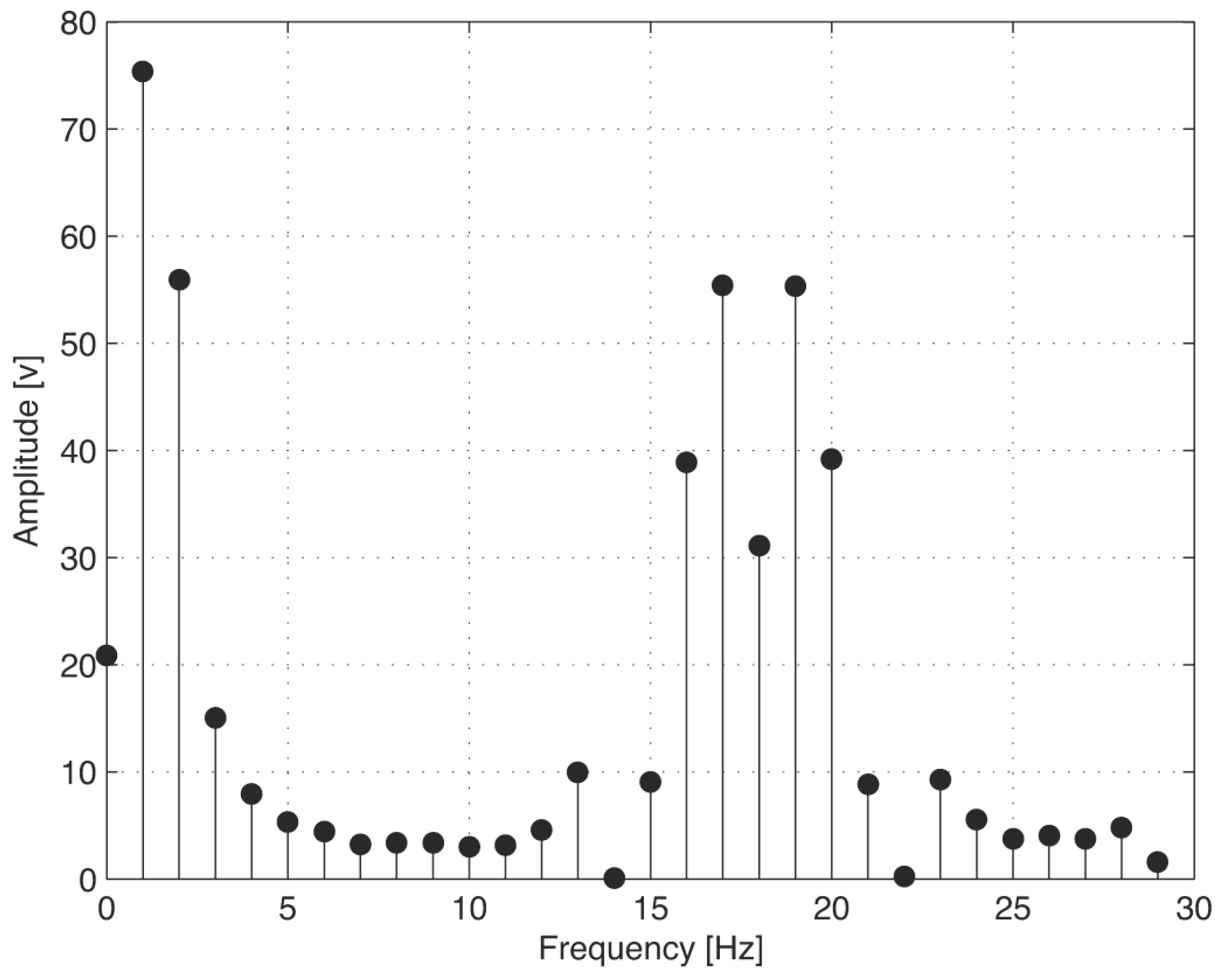
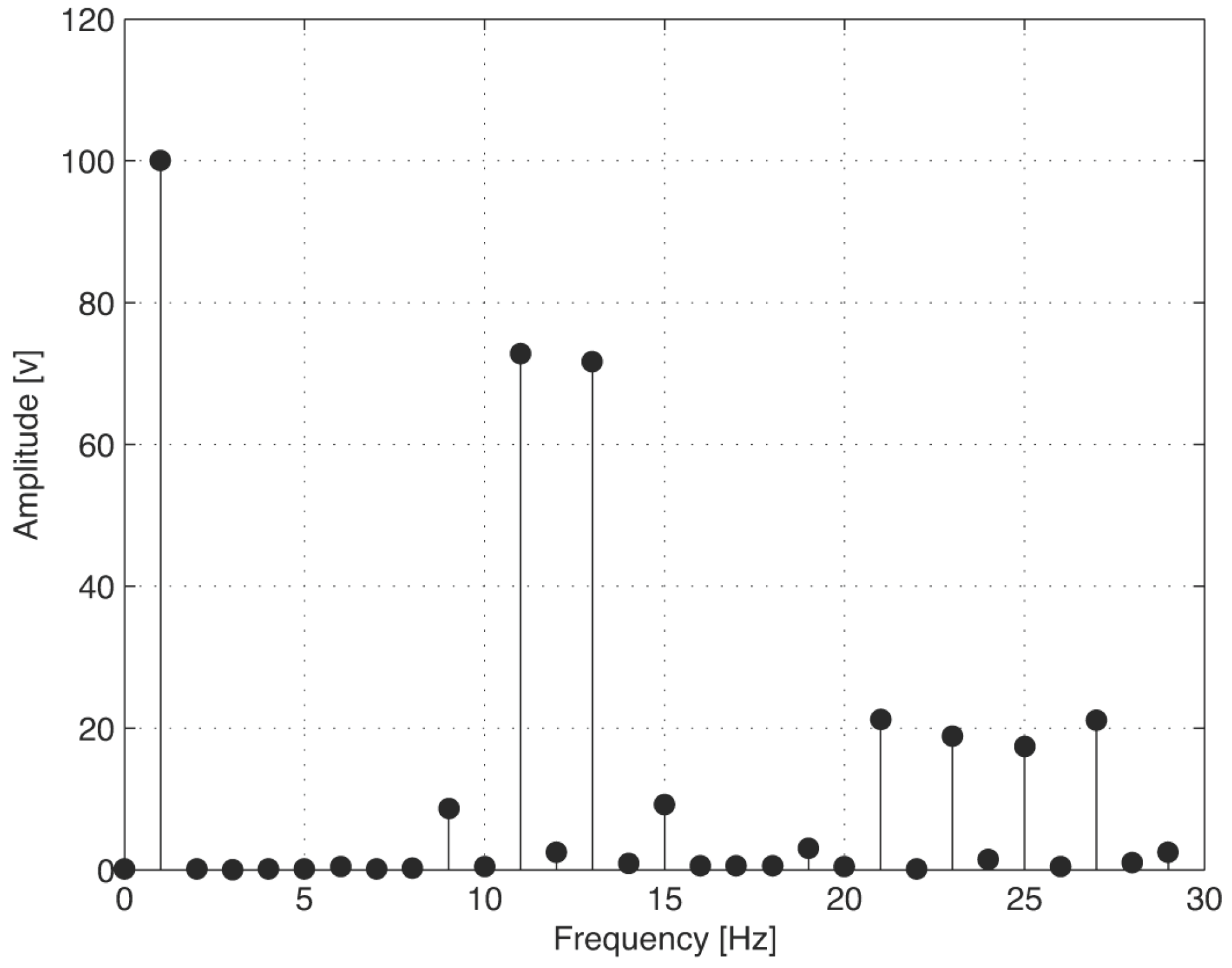
2.1. Analysis of the Spectrum Leakage at Sinusoidal Signals
2.2. Acquisition of a Signal Time-Lapse
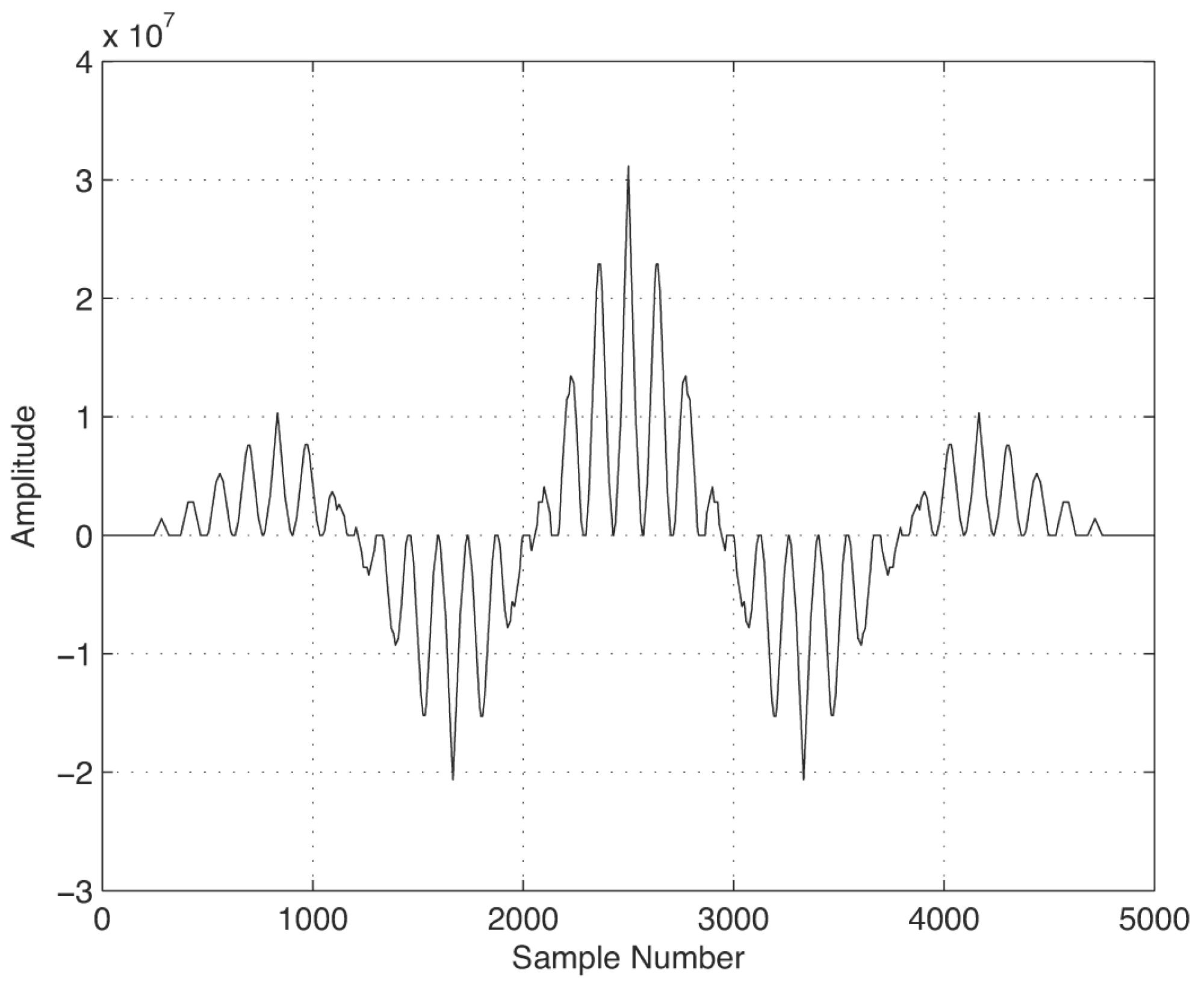
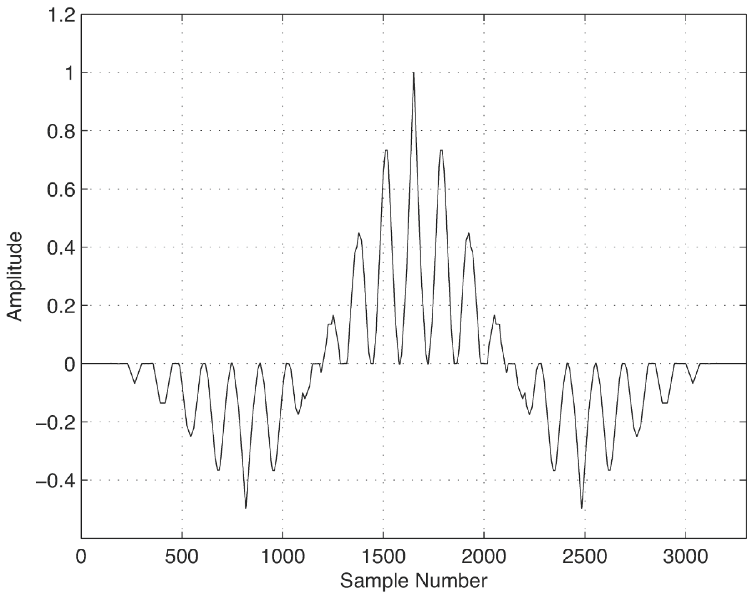
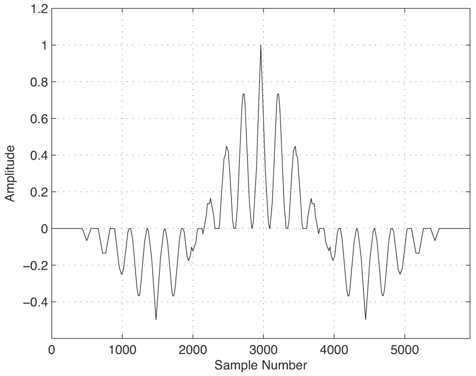
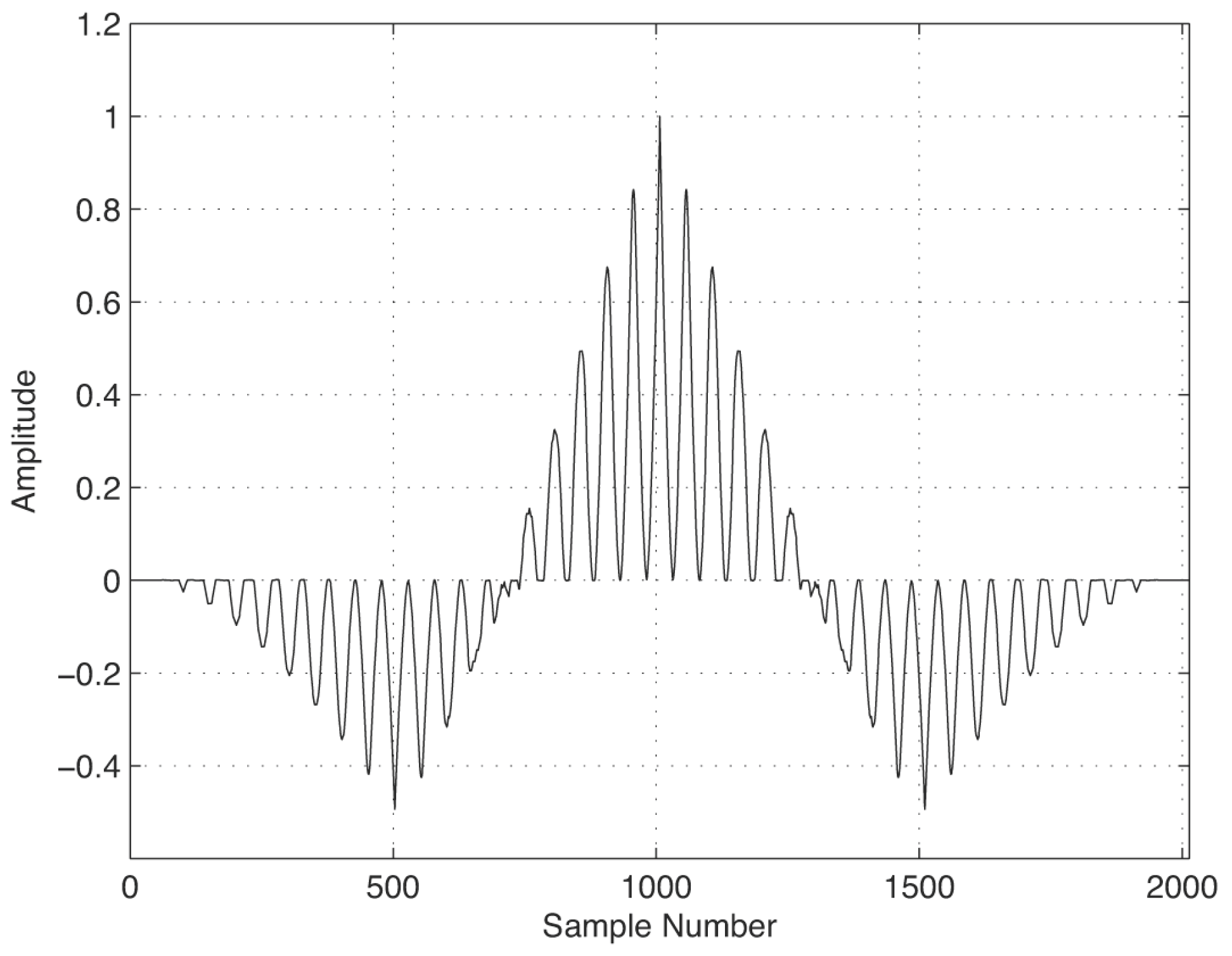
2.3. The Autocorrelation Function
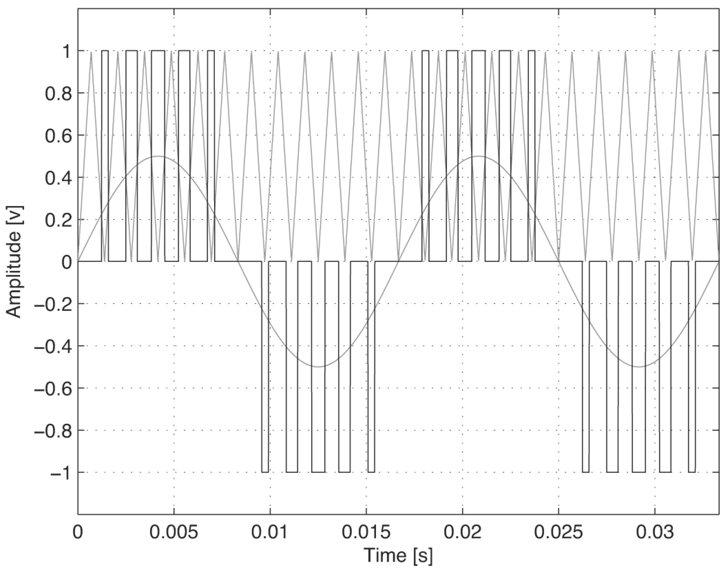
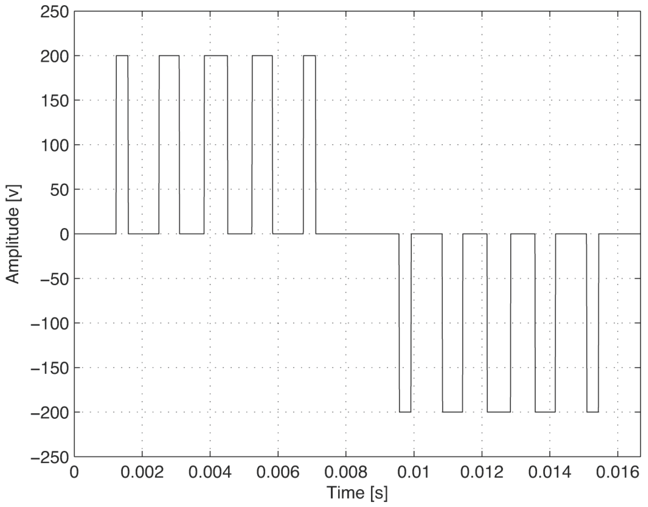
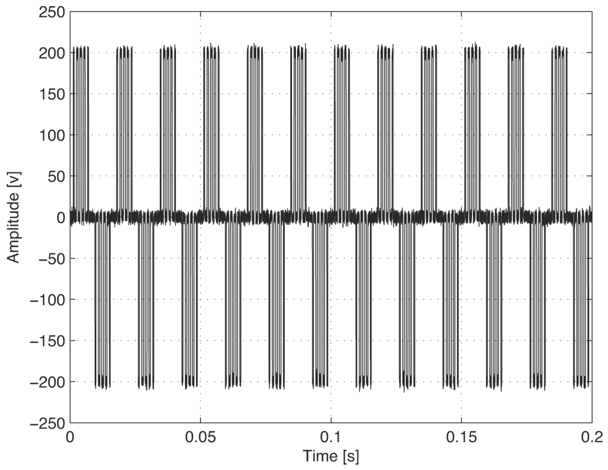
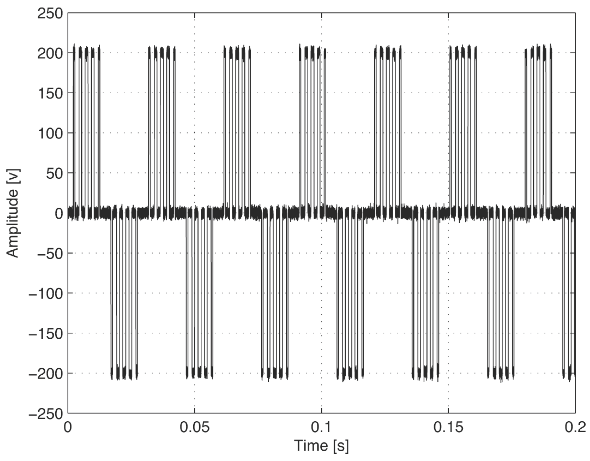
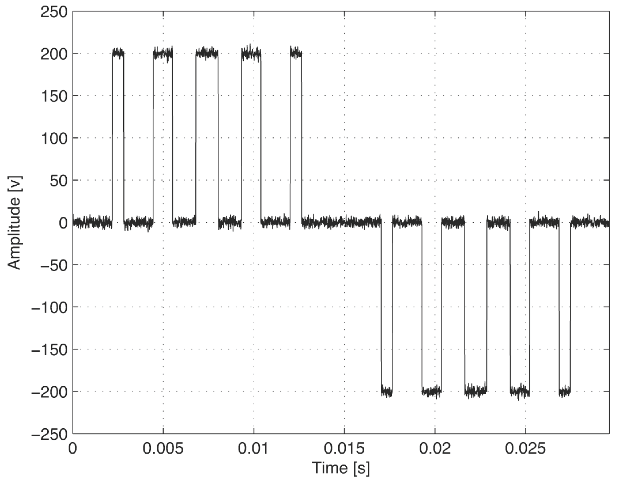
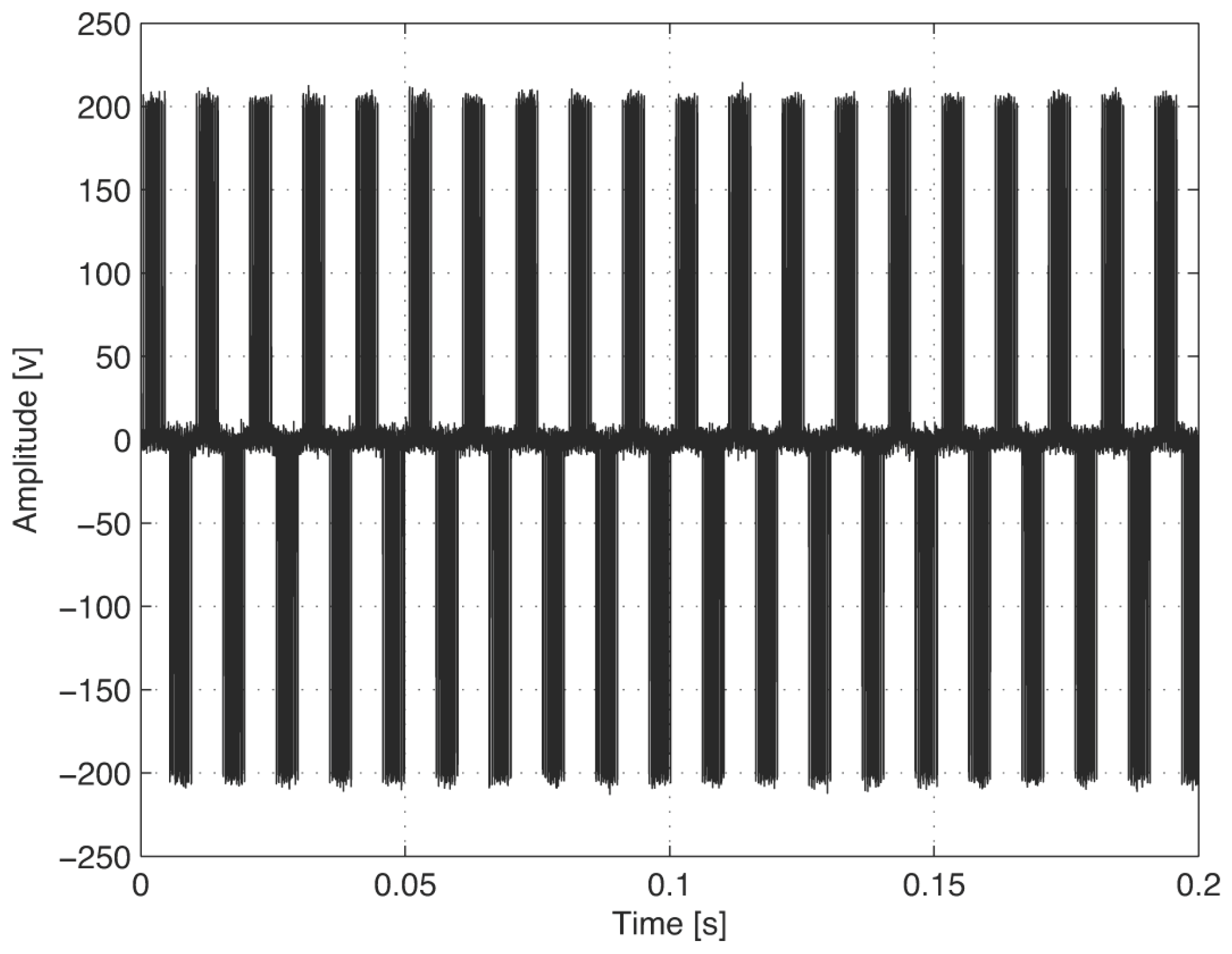
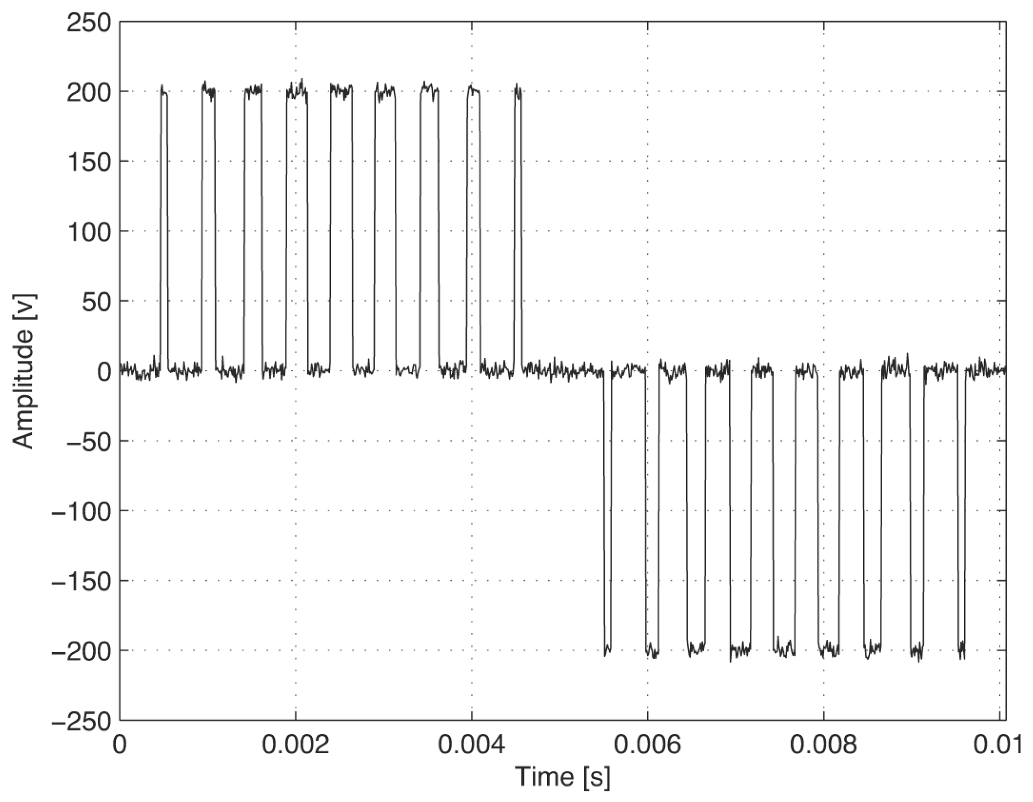
2.4. The Sinusoidal Pulse Width Modulation
3. Automatic Fourier Spectrum Detection Using Autocorrelation
- (1)
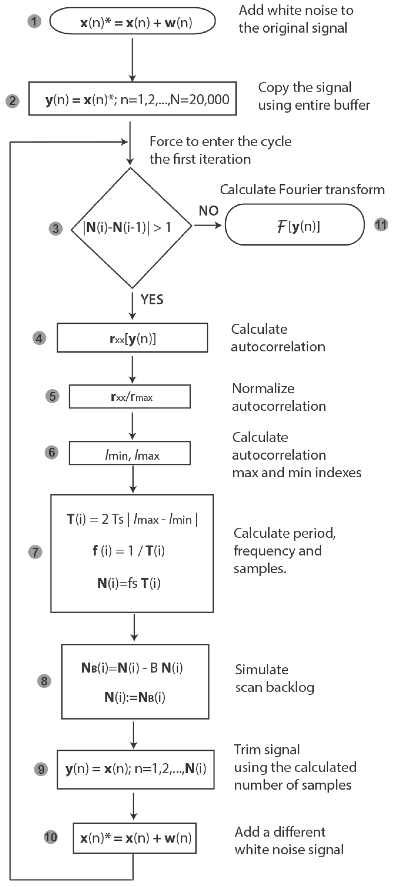
- In this step, a white noise signal is added to the original SPWM signal to simulate the effect of the acquisition noise.
- (2)
- Initially, because there is no information about the signal frequency, the algorithm retrieves the entire buffer to obtain a first approximation. In this step, the scan backlog is neglected because the sample loss is irrelevant.
- (3)
- After being forced to enter the cycle for the first iteration, the algorithm compares the last two values regarding the number of samples needed to represent a single period. If these values differ for more than one sample, then the algorithm continues with the calculation; else, the Fourier spectrum is computed and displayed as indicated by Step 11.
- (4)
- The signal autocorrelation is calculated. If this is the first iteration, the autocorrelation is calculated for the 20 Ksamples; else, a trimmed version of the signal is used.
- (5)
- The result of the autocorrelation is normalized in order to maintain a constant size in the vertical axis of the screen.
- (6)
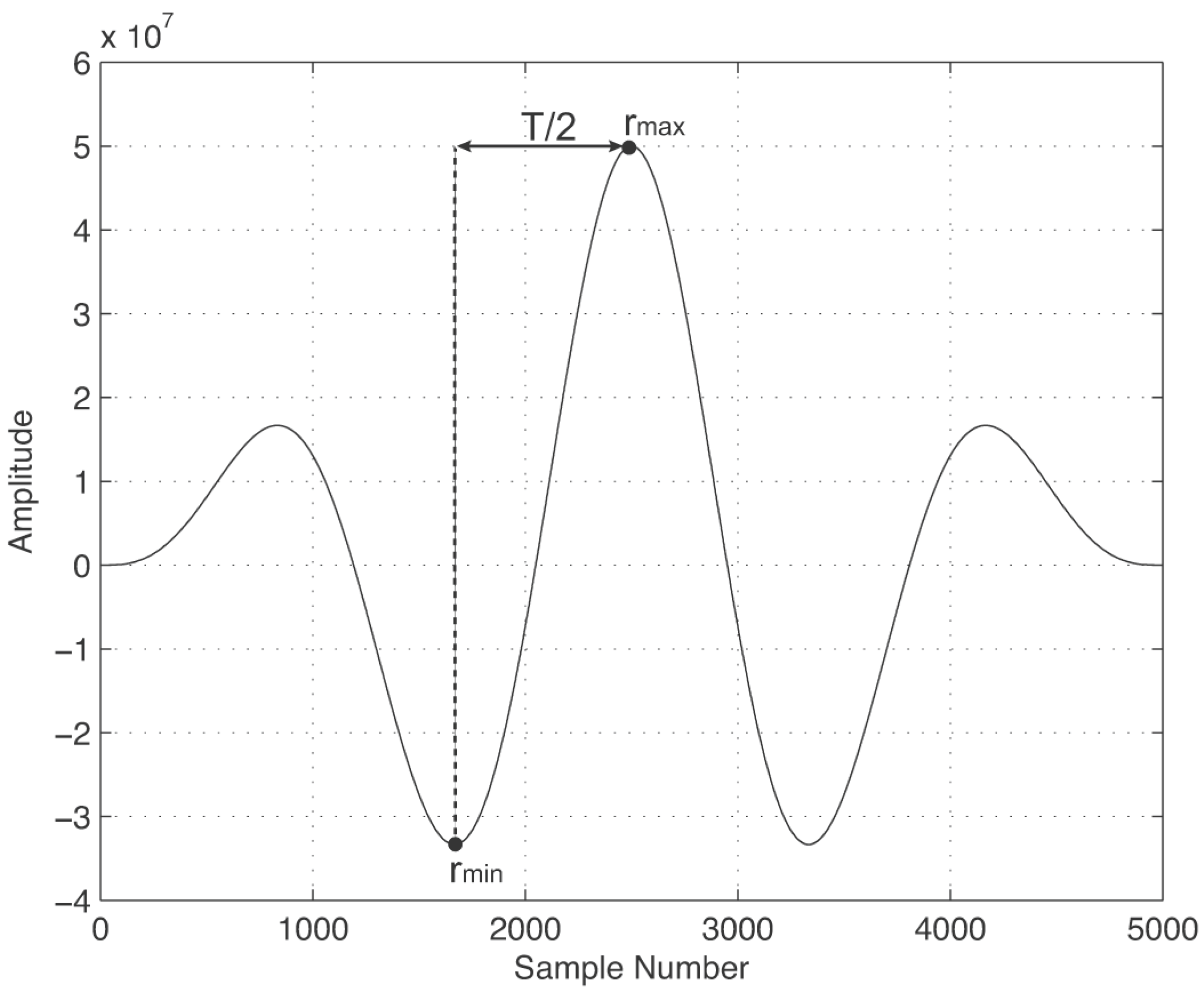
- The lag indexes for maximum and minimum values in the autocorrelation are obtained. This is achieved by using the MATLAB functions and , where X is a discrete sequence, M is the maximum or minimum value (according to the function used) and I is the index where the value of interest is located.
- (7)
- (8)
- In this step, a simulation of the scan backlog effect is considered. The scan backlog indicates how much data remain in the buffer after each retrieval, providing a measure of how well the application is maintaining the throughput rate [20,23]; i.e., a Data Acquisition Card (DAQ) does not retrieve the data at the same rate as the sampling frequency . The retrieval speed refers to how fast the computer is taking samples from the buffer toward a specific application.In this simulation, we assume a constant sampling frequency; hence, all of the samples are separated by a time interval of regardless of the retrieval speed.Equation (18) shows our proposed model of the scan backlog. The scan backlog factor B is treated as a random variable that follows a uniform distribution; i.e., B~u(0,0.01). Therefore, the acquired number of N samples is reduced by 1% towards the actual number of samples processed in the worst case. For example, a number of samples less than or equal to 200 samples can be lost from a total of 20 K samples.
- (9)
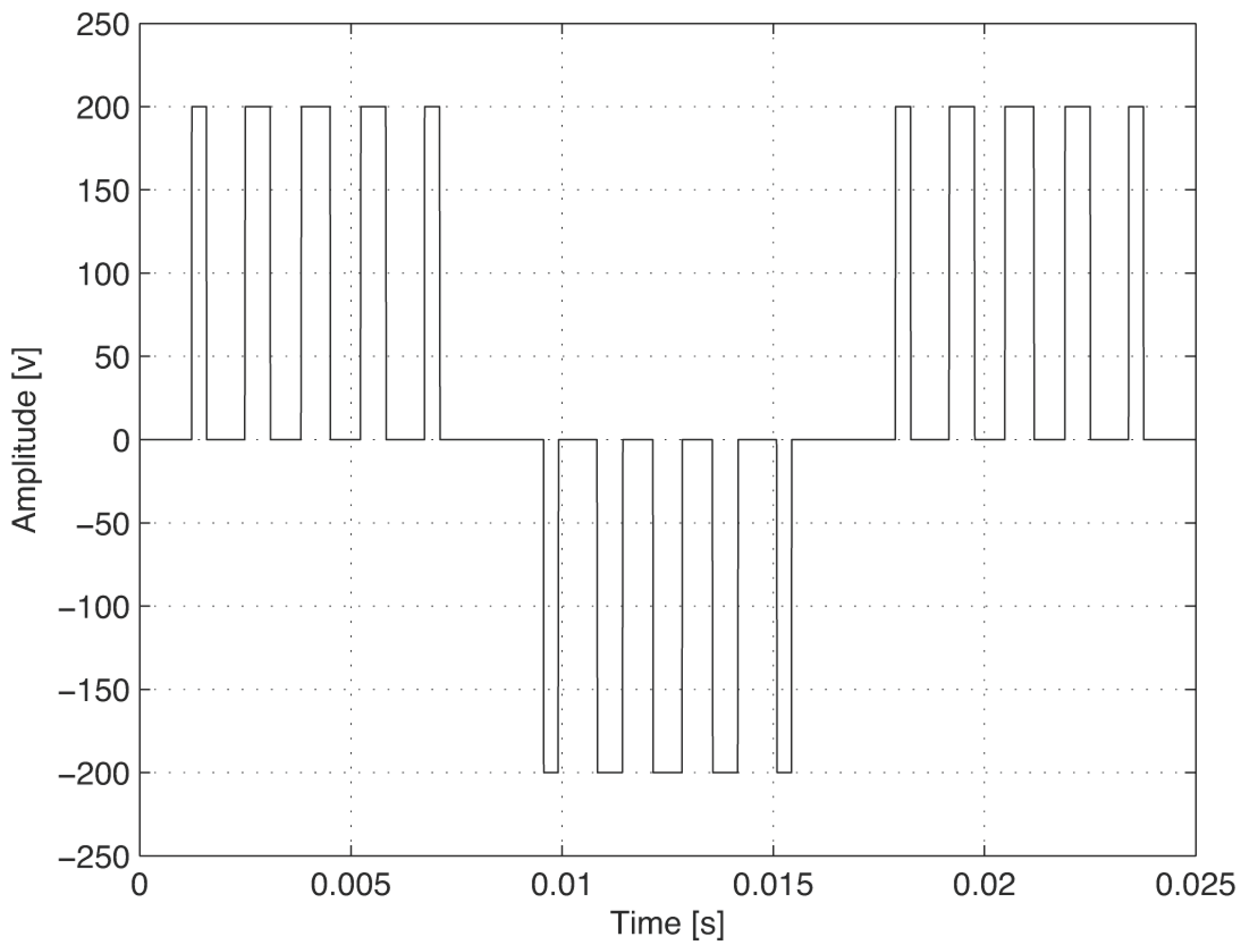
- In this step, the original digital sequence is trimmed according to the computed number of samples necessary to represent a single cycle; however, this parameter is affected by the scan backlog effect; therefore, the algorithm needs at least two iterations to decide if the computed number of samples is correct.
- (10)
- In this step, a white-noise signal with a signal to noise ratio dB is added to the acquired SPWM signal to model the acquisition noise. In every iteration, a different white noise signal is used because the computer must simulate the start of a new acquisition.
4. Algorithm Evaluation Methodology
5. Conclusions and Future Work
- It is important to represent a single SPWM signal period in the Fourier analysis; otherwise, the amplitude non-existing harmonics could lead to a poor electrical diagnosis. In industry, this could affect the preventive and corrective actions taken regarding the AC motors and their drives.
- The autocorrelation function can be applied to calculate the period of SPMW signals regardless of the magnitude of the pattern of pulses.
- The autocorrelation function can be used to estimate the period of SPWM signals under the loss of samples.
- The acquisition noise had no substantial effect in the calculation of the required number of samples.
- Taking advantage of the symmetry of the autocorrelation, we have searched for the maximum and minimum value indexes regardless of the global maximum and minimum locations. This allowed for a rapid estimation of the signal period.
- We have provided a simple stochastic model for the scan backlog, to analyze the sample loss.
- We have implemented an algorithm that uses the autocorrelation to iteratively calculate an SPWM signal period despite the loss of samples and acquisition noise. Thus, we have provided a simulation under realistic conditions for an acquisition process.
- The scan backlog can also be modeled with variations in the sampling frequency around a set point.
- In this study, the acquisition process commenced at the beginning of the positive semi-cycle; however, the variation of a specified trigger level can also be analyzed.
- The analysis of other PWM techniques using this algorithm is encouraged.
- The proposed algorithm can be programmed into a real acquisition device to analyze SPWM voltage and current signals.
Acknowledgments
Author Contributions
Conflicts of Interest
Appendix A


Appendix B
References
- Reza, S.E. A Study on SPWM Boost Inverter and Its Reactive Power Control Strategy; Lap Lambert Academic Publishing: Saarbrücken, Germany, 2012; pp. 12–19. [Google Scholar]
- Rapuano, S.; Harris, F.J. An Introduction to FFT and Time Domain Windows. IEEE Trans. Instrum. Meas. 2007, 10, 32–44. [Google Scholar] [CrossRef]
- Chugani, M.L.; Samant, A.R.; Cerna, M. LabView Signal Processing; Prentice Hall PTR: Upper Saddle River, NJ, USA, 1998; pp. 76–104. [Google Scholar]
- Rashid, M.H. Power Electronics: Circuits, Devices and Applications; Pearson Prentice Hall: Upper Saddle River, NJ, USA, 2004; pp. 253–256. [Google Scholar]
- Mohan, N.; Undeland, T.M.; Robbins, W.P. Power Electronics: Converters, Applications and Design; John Wiley and Sons, Inc.: Hoboken, NJ, USA, 2003; pp. 212–216. [Google Scholar]
- Brown, M. Power Electronics in Motor Drives; Elektor International Media: London, UK, 2010; pp. 92–95. [Google Scholar]
- Llamas, A.; Acevedo, S.; Baez, J.A.; Reyes, J.A. Armónicas en Sistemas Eléctricos Industriales; Innovación Editorial Lagares: Monterrey, México, 2004; pp. 56–59. [Google Scholar]
- Nam, S.; Kang, S.; Kang, S. Real-Time Estimation of Power System Frequency Using A Three-Level Discrete Fourier Transform Method. Energies 2014, 8, 79–93. [Google Scholar] [CrossRef]
- Proakis, J.G.; Manolakis, D.G. Digital Signal Processing; Pearson Prentice Hall: Madrid, Spain, 2007; pp. 109–457. [Google Scholar]
- Rabiner, L.R. On the Use of Autocorrelation Analysis for Pitch Detection. IEEE Trans. Acoust. Speech Signal Process. 1977, 25, 24–33. [Google Scholar] [CrossRef]
- Shahnaz, C.; Zhu, W.; Ahmad, M.O. Pitch Estimation Based on a Harmonic Sinusoidal Autocorrelation Model and a Time-Domain Matching Scheme. IEEE Trans. Audio Speech Lang. Process. 2012, 20, 310–323. [Google Scholar] [CrossRef]
- Xiao, Y.; Wei, P.; Tai, H. Autocorrelation-Based algorithm for single-frequency estimation. Signal Process. 2007, 87, 1224–1233. [Google Scholar] [CrossRef]
- Elasmi-Ksibi, R.; Besbes, H.; López-Valcarce, R.; Cherif, S. Frequency estimation of real-valued single-tone in colored noise using multiple autocorrelation lags. Signal Process. 2010, 90, 2303–2307. [Google Scholar] [CrossRef]
- Cao, Y.; Wei, G.; Chen, F.A. A closed-form expanded autocorrelation method for frequency estimation of a sinusoid. Signal Process. 2012, 92, 885–892. [Google Scholar] [CrossRef]
- Stoica, P.; Randolph, L.M. Spectral Analysis of Signals; Pearson Prentice Hall: Upper Saddle River, NJ, USA, 2005. [Google Scholar]
- Hayes, M.H. Statistical Digital Signal Processing and Modeling; John Wiley and Sons: New York, NY, USA, 2009. [Google Scholar]
- Parker, B.J.; Luenberger, D.G.; Wenger, D.L. Estimation of structured covariance matrices. Proc. IEEE 1982, 70, 963–974. [Google Scholar]
- Zorzi, M.; Ferrante, A. On the estimation of structured covariance matrices. Automatica 2012, 48, 2145–2151. [Google Scholar] [CrossRef]
- Cai, T.T.; Ren, Z.; Zhou, H.H. Estimating structured high-dimensional covariance and precision matrices: Optimal rates and adaptive estimation. Electr. J. Stat. 2016, 10, 1–59. [Google Scholar] [CrossRef]
- Eltahir, W.E.; Lai, W.K.; Ismail, A.F.; Salami, M.J. Hardware Design, Development and Evaluation of a Pressure-based Typing Biometrics Authentication System. In Proceedings of the Eighth Australian and New Zealand Intelligent Information Systems Conference (ANZIIS), Sidney, Australia, 10–12 December 2003; pp. 49–54.
- Wei, C.; Zhuang, Z. A CAN Network for Temperature Monitoring of Car Engine and Train Bogie. In Proceedings of the International Conference on Internet Computing and Information Services, (ICICIS), Hong Kong, China, 17–18 September 2011; pp. 302–305.
- Skibinski, G.L.; Kerkman, R.J.; Schlegel, D. EMI emissions of modern PWM AC drives. IEEE Trans. Ind. Appl. 1999, 5, 47–81. [Google Scholar] [CrossRef]
- Rabiner, L.; Cooley, J.; Helms, H.; Jackson, L.; Kaiser, J. Terminology in digital signal processing. IEEE Trans. Audio Electroacoust. 1972, 20, 322–337. [Google Scholar] [CrossRef]
- Prandoni, P.; Vetterli, M. Signal Processing for Communications; CRC Press: Boca Raton, FL, USA, 2008; pp. 63–65. [Google Scholar]
- Matlab. The MathWorks, Inc. Available online: http://www.mathworks.com/ (accessed on 16 July 2016).
- Yue, X.; Ma, X.; Wang, H. A conceit of unipolar N-multiple frequency SPWM and the main circuit topology. In Proceedings of the IEEE 6th International Power Electronics and Motion Control Conference, Wuhan, China, 17–20 May 2009; pp. 1531–1534.
- Patel, M.A.; Patel, A.R.; Vyas, D.R.; Patel, K.M. Use of PWM techniques for power quality improvement. J. Recent Trends Eng. Technol. 2009, 1, 99–102. [Google Scholar]


© 2016 by the authors; licensee MDPI, Basel, Switzerland. This article is an open access article distributed under the terms and conditions of the Creative Commons Attribution (CC-BY) license (http://creativecommons.org/licenses/by/4.0/).
Share and Cite
Said, A.; Davizón, Y.A.; Espino-Román, P.; Rodríguez-Said, R.; Hernández-Santos, C. Automatic Frequency Identification under Sample Loss in Sinusoidal Pulse Width Modulation Signals Using an Iterative Autocorrelation Algorithm. Symmetry 2016, 8, 78. https://doi.org/10.3390/sym8080078
Said A, Davizón YA, Espino-Román P, Rodríguez-Said R, Hernández-Santos C. Automatic Frequency Identification under Sample Loss in Sinusoidal Pulse Width Modulation Signals Using an Iterative Autocorrelation Algorithm. Symmetry. 2016; 8(8):78. https://doi.org/10.3390/sym8080078
Chicago/Turabian StyleSaid, Alejandro, Yasser A. Davizón, Piero Espino-Román, Roberto Rodríguez-Said, and Carlos Hernández-Santos. 2016. "Automatic Frequency Identification under Sample Loss in Sinusoidal Pulse Width Modulation Signals Using an Iterative Autocorrelation Algorithm" Symmetry 8, no. 8: 78. https://doi.org/10.3390/sym8080078