Linear Recurrent Double Sequences with Constant Border in M₂(F₂) are Classified According to Their Geometric Content

Abstract

The author used the automatic proof procedure introduced in [1] and verified that the 4096 homomorphic recurrent double sequences with constant borders defined over Klein’s Vierergruppe $\mathbb{K}$ and the 4096 linear recurrent double sequences with constant border defined over the matrix ring $M_2\left({\mathbb{F}}_2\right)$ can be also produced by systems of substitutions with finitely many rules. This permits the definition of a sound notion of geometric content for most of these sequences, more exactly for those which are not primitive. We group the 4096 many linear recurrent double sequences with constant border I over the ring $M_2\left({\mathbb{F}}_2\right)$ in 90 geometric types. The classification over Klein’s Vierergruppe $\mathbb{K}$ is not explicitly displayed and consists of the same geometric types like for $M_2\left({\mathbb{F}}_2\right)$, but contains more exceptions. There are a lot of cases of unsymmetric double sequences converging to symmetric geometric contents. We display also geometric types occurring both in a monochromatic and in a dichromatic version.

1. Introduction

Recurrent double sequences are double sequences $a:{\mathbb{N}}^2\to A$ which are defined by initial conditions $a(i,0)=g\left(i\right)$, $a(0,j)=h\left(j\right)$ and by a recurrence $a(i,j)=f\left(a\right(i,j-1),a(i-1,j-1)$, $a(i-1,j))$. The author proved in [2] that recurrent double sequences with finite alphabets A and constant initial conditions are Turing-complete. Other recurrent double sequences of interest are those which are self-similar, like some sequences given by linear recurrences studied in [3], where a conjecture first appeared in [4] has been solved. Continuing on this direction, the author has found an automatic proof method able to prove that some concrete recurrent double sequences can be also obtained by systems of substitutions [1], and applied it also for some recurrent double sequences with periodic (instead of constant) initial conditions [5]. Although not all recurrent double sequences can be alternatively generated by systems of substitutions, as shown in [6], it is interesting to find out more about those doing so. After a big number of experiments the author conjectured that for all finite Abelian groups G, all homomorphisms $f:G^3\to G$ and all periodic initial conditions $g,h:\mathbb{N}\to G$, the resulting recurrent double sequence can also be generated by an system of substitutions.

At the beginning of this research, we have verified the Abelian group conjecture for the group $G=\mathbb{K}={\mathbb{F}}_2\times {\mathbb{F}}_2$, Klein’s four-element group, also called here (like in German) Klein’s Vierergruppe. We think that $\mathbb{K}$ is an example of interest, because $\mathbb{K}$ is the smallest non-cyclic group. All the 4096 recurrent double sequences defined by homomorphisms of ${\mathbb{K}}^3$ in $\mathbb{K}$ and starting with constant initial conditions $g\equiv h\equiv (1,0)$ proved to be also generated by systems of substitutions. Most of them are generated by systems of type $2\to 4$, but there are some needing $4\to 8$, $2\to 8$ or $3\to 6$. The notation $x\to sx$ used here has been already used by the author in [1,5,6] and will be explained again with details and some examples in the present paper. Roughly, it says that we are concerned with substitution rules in which $x\times x$ square matrices are substituted with $sx\times sx$ square matrices. Those bigger matrices are composed by $s\times s$ blocks, each of those blocks being a $x\times x$ matrix found as the left hand side of a substitution rule. In this way the process of substitution starting with one $x\times x$ matrix that is the left hand side of a substitution rule can continue indefinitely. In our case only expansive systems of substitution are useful: in these systems of substitution the starting $x\times x$ matrix is substituted by a $sx\times sx$ matrix, whose left-upper $x\times x$ sub-block is again the starting matrix. If this condition is fulfilled, every production of a substitution step is the corresponding left-upper minor of its successor, as one can immediately see by induction.

The number of rules in the systems of substitutions occurring in the present article varies from one to more than one hundred.

The mathematical topics related with the phenomenon studied here belong to a large emerging mathematical movement. Although the first problems of this kind occurred in the nineteenth century with the Prouhet Sequence (see [7,8]; the sequence has been rediscovered by Axel Thue and Marston Morse and is currently called the Thue–Morse sequence) or even long time before with numeric recurrent sequences like Fibonacci’s Sequence or Pascal’s Triangle (see [9]), this complex and still crystallizing direction of research, which mixes up elements of discrete and continuous mathematics and touches fractals, aperiodic tilings, cellular automata, Lindenmayer systems, quasicrystals, mathematical diffraction, but also number theory (like Collatz’ Problem) and combinatorics, exploded in the second half of the twentieth century and form one of the main lines of feed-back in pure science produced by the applied one, specially by the development of computers. Being still in a crystallization process, it is difficult to speak about one big source of reference for this dynamic field of research. However, one can recall some works that became important references in special sub-fields. The recurrent double sequences defined by the more rudimentary rule of recurrence $a(i,j)=f\left(a\right(i-1,j),a(i,j-1\left)\right)$ are time diagrams of one-dimensional cellular automata. To see classical studies concerning time-diagrams of cellular automata and fractals, read the Wilson’s paper [10], Mandelbrot’s celebrated monograph [11] or the survey by Kari [12]. Other time-diagrams of Turing machines and a lot of phenomena present also in general recurrent double sequences have been described by Stephen Wolfram in his exceptional monograph “A new kind of science”, see [13]. The substitution for one-dimensional sequences is very well treated in the survey [9] by Muchnik and coauthors, and in the monograph [7] by Allouche and Shallit. The substitution had a sensational come-back in geometry by the discovery of Penrose’ aperiodic tilings [14], although other works concerning aperiodic tilings have already used it before—notably by Wang [15] and Raphael Robinson [16]. For substitution in tilings see also the monograph [17]. The abstract idea of substitution is essentially present in Lindenmayer Systems, a discrete work tool able to analyze morphogenesis in plants and the structure of quasicrystals [18,19]. For further applications and developments concerning substitution there is a huge literature on quasicrystals and mathematical diffraction. We cite here only [20] and [21].

Definition 1.1

The homomorphisms $h:\mathbb{K}\to \mathbb{K}$ itself are functions given by $h(\overrightarrow{x})=A·{\overrightarrow{x}}^T$, with $A\in M_2\left({\mathbb{F}}_2\right)$. The homomorphisms of groups $f:{\mathbb{K}}^3\to \mathbb{K}$ have the form

$$f(\overrightarrow{x},\overrightarrow{y},\overrightarrow{z})=A·{\overrightarrow{x}}^T+B·{\overrightarrow{y}}^T+C·{\overrightarrow{z}}^T$$

where $A,B,C\in M_2\left({\mathbb{F}}_2\right)$ are matrices. We identify the homomorphism $f:{\mathbb{K}}^3\to \mathbb{K}$ with the triple $ABC\in M_2{\left({\mathbb{F}}_2\right)}^3$

Definition 1.2

The matrix ring $M_2\left({\mathbb{F}}_2\right)$ contains 16 elements and it is necessary to have a fixed notation for each of them. If we write down the matrix

$$\left(\begin{array}{cc}{x}_1& x_2\\ x_3& x_4\end{array}\right)$$

as $x_1{x}_2{x}_3{x}_4$, then we call: $o=0000$, $u=0100$, $v=0010$, $z=1111$, $a=1100$, $b=0011$, $c=1010$, $d=0101$, $e=1000$, $f=0001$, $I=1001$, $J=0110$, $K=1011$, $L=1101$, $X=0111$, $Y=1110$.

The matrices $\{I,J,K,L,X,Y\}$ are exactly the invertible matrices in $M_2\left({\mathbb{F}}_2\right)$. So those 6 matrices build together the group $G{L}_2\left({\mathbb{F}}_2\right)$ of the isomorphisms of $\mathbb{K}$ seen as an ${\mathbb{F}}_2$-vector space. $G{L}_2\left({\mathbb{F}}_2\right)$ is isomorphic with $S_3$, the group of all permutations of three objects. Indeed, $G{L}_2\left({\mathbb{F}}_2\right)$ acts on the three non-zero elements of the group $\mathbb{K}$ such that every permutation of them can be trivially extended to a linear application. I is the identity, J, K and L correspond to two-element transpositions and have order two, and X, Y correspond to 3-cyclic permutations and have order three. The partition $\left\{I\right\}\cup \{J,K,L\}\cup \{X,Y\}$ is the decomposition of $G{L}_2\left({\mathbb{F}}_2\right)$ in classes of conjugation, according to the theory of groups. It will be useful to extend this partition to a partition of the whole ring $M_2\left({\mathbb{F}}_2\right)$ in classes of conjugation.

Definition 1.3

Let $R=(R,+,·,0,1)$ be a ring and $R^{\times }=(R^{\times },·,1)$ be its multiplicative group of units. Two elements $x,y\in R$ are called conjugated if and only if there is some $\phi \in R^{\times }$ such that $y={\phi }^{-1}x\phi$. In this situation we write $y=x^{\phi }$.

We observe that the conjugation is a relation of equivalence in R. Consequently, $\widehat{x}:=x^{R^{\times }}=\left\{{\phi }^{-1}x\phi \right|\phi \in R^{\times }\}$ is the class of conjugation of x. If $R=M_2\left({\mathbb{F}}_2\right)$, then $R^{\times }=G{L}_2\left({\mathbb{F}}_2\right)$ and R decomposes in classes of conjugation as follows:

$$R=\left\{I\right\}\cup \{J,K,L\}\cup \{X,Y\}\cup \{a,b,c,d,e,f\}\cup \{u,v,z\}\cup \left\{o\right\}$$

Denote by $\widehat{y}$ the conjugation class of y. We observe that $\widehat{a}=\{x\in R|x^2=x\}$ collects all the idempotents, and $\widehat{z}=\{x\in R\backslash \left\{0\right\}|x^2=0\}$ collects all the non-zero nilpotents.

Definition 1.4

Let $f:{\mathbb{K}}^3\to \mathbb{K}$ be a homomorphism of groups and $\phi \in G{L}_2\left({\mathbb{F}}_2\right)$. We call ${\phi }^{-1}\circ f\circ (\phi ,\phi ,\phi ):=f^{\phi }$ the conjugated of f by $\phi$. We observe that $f^{\phi }:{\mathbb{K}}^3\to \mathbb{K}$ is itself a homomorphism of groups.

If $f=ABC$ then $f^{\phi }=A^{\phi }{C}^{\phi }{D}^{\phi }$. The conjugation class of f shall be denoted by $\widehat{f}=\widehat{ABC}$ and is the set $\left\{f^{\phi }\right|\phi \in G{L}_2\left({\mathbb{F}}_2\right)\}$.

Definition 1.5

Let M and N be two sets and $a:{\mathbb{N}}^2\to M$, $b:{\mathbb{N}}^2\to N$ be two double sequences. Let $\mu :{\mathbb{N}}^2\to {\mathbb{N}}^2$ be the mirroring $\mu (x,y)=(y,x)$, and $id:{\mathbb{N}}^2\to {\mathbb{N}}^2$ be the identity. We say that a and b are isomorphic if and only if there is a bijection $\iota :a\left({\mathbb{N}}^2\right)\to b\left({\mathbb{N}}^2\right)$ and a function $\nu \in \{\mu ,id\}$ such that for all $i,j\in \mathbb{N}$, $\iota \left(a\right(i,j\left)\right)=b\left(\nu \right(i,j\left)\right)$.

Lemma 1.6

Let $x_0\in K\backslash \left\{0\right\}$ be an element, $f:{\mathbb{K}}^3\to \mathbb{K}$ a homomorphism of groups, and $\phi \in G{L}_2\left({\mathbb{F}}_2\right)$ an automorphism of $\mathbb{K}$. Let a be the recurrent double sequence generated by f with initial conditions $a(i,0)=a(0,j)=x_0$ and b the recurrent double sequence generated by $f^{\phi }$ with initial conditions $b(i,0)=b(0,j)={\phi }^{-1}\left(x_0\right)$. Then a and b are isomorphic. Consequently, in order to make a geometric classification of the homomorphic recurrent double sequences of Klein’s Vieregruppe $\mathbb{K}$ with constant initial conditions, it is sufficient to consider only one value for the initial conditions, like $x_0=(1,0)$.

Proof: 

One immediately proves by induction that for all $i,j\in \mathbb{N}$, $a(i,j)=\phi \left(b\right(i,j\left)\right)$. But $\phi :\mathbb{K}\to \mathbb{K}$ is a bijection, and the restriction to $b\left({\mathbb{N}}^2\right)$ is also a bijection with its own image, so the recurrent double sequences are isomorphic.   □

For the homomorphic recurrent double sequences with initial value $x_0=(1,0)$ over $\mathbb{K}$ we observed the following facts:

• A recurrent double sequence remains constant if and only if it satisfies the relation $f(x_0,x_0,x_0)=x_0$ for $x_0=(1,0)$. Exactly 1024 sequences, i.e., a quarter of 4096, are constant.
• All homomorphic recurrent double sequences over $\mathbb{K}$ can be also generated by systems of substitutions. Moreover, most of them can be easily associated a geometric content, and there are only 90 such contents occurring in the 4096 homomorphisms.
• Recurrent double sequences produced by homomorphisms lying in the same class of conjugation (tend to) have the same geometric content. This fact is at the first sight a surprise, and was not foreseen by Lemma 1.6. Moreover there are two different kinds of exceptions:

  A

  A normal exception is the situation when two homomorphisms in a class of conjugation of six homomorphisms or one homomorphism in a class of conjugation of three homomorphisms produce a constant recurrent double sequence, although the other homomorphisms in the class of conjugation remain in the same (non-uniform) type.

  B

  A sporadic exception is the situation in which some recurrent double sequences with different geometric content are produced by conjugated homomorphisms. Only some few classes of conjugation (only 33 classes in 736) split in different geometric contents. Pairs of contents occurring in sporadic exceptions are from sets that were called later type 1 and type 2, type 2 and type 19, type 19 and 74, type 2 and type 74. See the Classification for the definition of those geometric types.

These exceptions made clear that the appropriate structure to make a geometric classification of the recurrent double sequences is not Klein’s Vieregruppe $\mathbb{K}$ with the homomorphisms $f:{\mathbb{K}}^3\to \mathbb{K}$, $f(x,y,z)=A·{\overrightarrow{x}}^T+B·{\overrightarrow{y}}^T+C·{\overrightarrow{z}}^T$ but the group $\mathbb{K}\times \mathbb{K}$ with the linear recurrence rules $F:{(\mathbb{K}\times \mathbb{K})}^3\to \mathbb{K}\times \mathbb{K}$, $F(X,Y,Z)=AX+BY+CZ$, where in both cases $A,B,C\in M_2\left({\mathbb{F}}_2\right)$. In order to understand this, $\mathbb{K}\times \mathbb{K}$ must be identified with the matrix group $M_2\left({\mathbb{F}}_2\right)$ itself, as it follows:

Definition 1.7

A matrix $A\in M_2\left({\mathbb{F}}_2\right)$ can be seen column-wise as a pair of elements of $\mathbb{K}$. For $i=1,2$ let ${\pi }_i:M_2\left({\mathbb{F}}_2\right)\to \mathbb{K}$ be the projection on column i: if $A=({\overrightarrow{c}}_1^T,{\overrightarrow{c}}_2^T)$ then ${\pi }_i\left(A\right)={\overrightarrow{c}}_i$. ${\pi }_i$ are homomorphisms of Abelian groups. If $\left(a(i,j)\right):{\mathbb{N}}^2\to M_2\left({\mathbb{F}}_2\right)$ is the linear recurrent double sequence over $M_2\left({\mathbb{F}}_2\right)$ with constant border $a(i,0)=a(0,j)=I$ and rule $a(i,j)=Aa(i,j-1)+Ba(i-1,j-1)+Ca(i-1,j)$ with some fixed $A,B,C\in M_2\left({\mathbb{F}}_2\right)$, then $b(i,j)={\pi }_1\left(a(i,j)\right)$ is the homomorphic recurrent double sequence over $\mathbb{K}$ with constant border $b(i,0)=b(0,j)=(1,0)$ and the same recurrence rule like $\left(a\right(i,j\left)\right)$.

If one graphically represents recurrent double sequences by square plots consisting of colored little squares, then the recurrent double sequences over $\mathbb{K}$ need at most four colors to be represented, while the linear recurrent double sequences over $M_2\left({\mathbb{F}}_2\right)$ need at most sixteen colors. One can imagine this construction in the following way: a homomorphic $\mathbb{K}$-sequence with border $(1,0)$ is paint on a transparent slide using a set of four distinct colors corresponding to the elements of $\mathbb{K}$. The homomorphic $\mathbb{K}$-sequence given by the same rule but with border $(0,1)$ is paint on another transparent slide using another set of four colors, which is disjoint from the set used before. If one overlaps the two slides, a maximum of sixteen colors can arise—if all pairs of colors do really occur in this overlapping. In fact the overlapping is the corresponding linear recurrent double sequence with border I over $M_2\left({\mathbb{F}}_2\right)$. This comparison is still not good enough, because a yellow and a blue overlapped slides mostly produce the same green if one reverses the overlapping, but $({{\overrightarrow{c}}_1}^T,{{\overrightarrow{c}}_2}^T)\ne ({{\overrightarrow{c}}_2}^T,{{\overrightarrow{c}}_1}^T)$ if ${\overrightarrow{c}}_1\ne {\overrightarrow{c}}_2$.

Observing the linear recurrent double sequences over $M_2\left({\mathbb{F}}_2\right)$, one finds out following:

• A linear recurrent double sequence over $M_2\left({\mathbb{F}}_2\right)$ remains constant if and only if it satisfies the relation $f(I,I,I)=I$. Exactly 256 sequences, i.e., $1/16$ of 4096, are constant. Moreover, the set of matrix triples producing constant sequences is a union of classes of conjugation of triples, because the given condition is compatible with the conjugation. Otherwise said, the normal exception noticed in $\mathbb{K}$ for homomorphic double sequences does not take place anymore.
• All linear recurrent double sequences over $\mathbb{K}$ can be also generated by systems of substitutions. Moreover, most of them can be easily associated with a geometric content, and there are only 90 such contents occurring in the 4096 homomorphisms. The geometric contents are very similar with those met in the homomorphic double sequences of $\mathbb{K}$. More on this is discussed in the third section.
• Recurrent double sequences produced by matrix triples lying in the same class of conjugation always have the same geometric content. More exactly, we will prove in the next section that homomorphisms lying in the same class of conjugation produce isomorphic recurrent double sequences over $M_2\left({\mathbb{F}}_2\right)$. Consequently, the fact that the geometric types are unions of classes of conjugation is no more surprising. Both the normal and the sporadic exceptions noticed in homomorphic double sequences over $\mathbb{K}$ completely disappear in $M_2\left({\mathbb{F}}_2\right)$. The sporadic exception was produced by the fact that the projection ${\pi }_1$ is sometimes bad and can map neighboring different elements from a double sequence onto neighboring equal elements in the other one.

We hope that this comparison between $\mathbb{K}$ and $M_2\left({\mathbb{F}}_2\right)$ completely justifies why we consider the ring $M_2\left({\mathbb{F}}_2\right)$ to be better than the group $\mathbb{K}$ in order to study and classify the homomorphic recurrent double sequences over $\mathbb{K}$.

2. Linear Recurrent Double Sequences Over Rings

In this section, $R=(R,+,·,0,1)$ is a ring with 1, not necessarily commutative or finite. $R^{\times }$ is the set of multiplicatively invertible elements (units of the ring). Always $1\in R^{\times }$ and $(R^{\times },·,1)$ is a group.

Definition 2.1

Let $A,B,C,x_0\in R$ be fixed elements. The linear recurrent double sequence with constant border over R defined by the tuple $(A,B,C,x_0)$ is a function $a:{\mathbb{N}}^2\to R$ satisfying the initial condition $a(i,0)=a(0,j)=x_0$ and the linear recurrence rule $a(i,j)=Aa(i,j-1)+Ba(i-1,j-1)+$ $Ca(i-1,j)$ for all $i,j\le 1$. We will use also the notation $(ABC,x_0)$ for the tuple defining the sequence.

There are many natural examples of linear recurrent double sequences. For $R=\mathbb{Z}$, the tuple $(1,0,1,1)$ defines a well-known recurrent double sequence called Pascal’s Triangle. Indeed, in this case $a(i,j)=\left(\genfrac{}{}{0pt}{}{i}{i+j}\right)$. For $p,k\in \mathbb{N}$, p prime, $k\ge 1$ and $R=\mathbb{Z}/p^k\mathbb{Z}$, one gets Pascal’s Triangle modulo $p^k$, which seems to always have a substitution structure—see [5], where we have studied some particular cases. In [1] we have studied the case of linear recurrent double sequences defined by the tuple $(1,m,1,1)$ for $R={\mathbb{F}}_q$, which is an arbitrary finite field of characteristic p with $q=p^k$ elements.

Definition 2.2

For a tuple $\overrightarrow{x}\in R^n$, $\overrightarrow{x}=(x_1,\cdots ,x_n)$ let $\widehat{\overrightarrow{x}}$ denote its class of conjugation relatively to the group of units of R:

$$\widehat{\overrightarrow{x}}=\widehat{(x_1,\cdots ,x_n)}=\left\{({\phi }^{-1}{x}_1\phi ,\cdots ,{\phi }^{-1}{x}_n\phi )\right|\phi \in R^{\times }\}$$

Only classes of conjugation $\widehat{a}$ for elements and $\widehat{ABC}$ for triples will occur here. The conjugate of the tuple $ABC$ by $\phi$ shall be also denoted ${\left[ABC\right]}^{\phi }$.

Lemma 2.3

Let $\phi \in R^{\times }$ be a unit. Then the mappings $m,c:R\to R$ given by $m\left(x\right)=x\phi$ and $c\left(x\right)=x^{\phi }={\phi }^{-1}x\phi$ are bijections.

Definition 2.4

Let A and B be two sets, $a:{\mathbb{N}}^2\to A$ and $b:{\mathbb{N}}^2\to B$ two double sequences. If there is a function $f:A\to B$ such that for all $i,j\in \mathbb{N}$, $b(i,j)=f\left(a\right(i,j\left)\right)$, we say that b is a projection of a and that f realizes a projection of a onto b.

For example the projections on the i-th column ${\pi }_i:M_2\left({\mathbb{F}}_2\right)\to \mathbb{K}$ defined in the Introduction realizes projections of linear recurrent double sequences in $M_2\left({\mathbb{F}}_2\right)$ onto homomorphic recurrent double sequences onto $\mathbb{K}$. Another natural projection is given in the next Corollary.

Corollary 2.5

Let R be an arbitrary ring with 1.

1.

Let $y\in R$ be an element. Then the recurrent double sequence defined by $(ABC,y)$ is the projection of the recurrent double sequence $(ABC,1)$ realized by the application $x⇝xy$. In particular, the recurrent double sequence defined by $(ABC,y)$ lives in the principal ideal $Ry$.

2.

Let $\phi ,\psi \in R^{\times }$ be units. Then the linear double sequences defined by $(ABC,1)$, $(ABC,\phi )$ and $({\left[ABC\right]}^{\phi },1)$ are isomorphic. They are also isomorphic with the linear double sequence defined by $({\left[ABC\right]}^{\phi },\psi )$.

3.

All recurrent double sequences $(DEF,1)$ produced by triples $DEF$ in some class of conjugation $\widehat{ABC}$ are isomorphic.

Proof: 

Let $s(i,j)$ be the sequence defined by $(ABC,1)$ and $t(i,j)$ be the recurrent double sequence defined by $(ABC,y)$. One shows by induction that for all $i,j\in \mathbb{N}$, $t(i,j)=s(i,j)y$. The first point is proved. For the second point: if now $t(i,j)$ is the sequence defined by $(ABC,\phi )$ and $u(i,j)$ is the sequence defined by $({\left[ABC\right]}^{\phi },1)$, we already know that $i,j\in \mathbb{N}$, $t(i,j)=s(i,j)\phi$ and we prove by induction that $u(i,j)=s{(i,j)}^{\phi }$. For both situations we apply now Lemma 2.3. The result for $({\left[ABC\right]}^{\phi },\psi )$ follows now by the transitivity of the isomorphism. The third point is only an emphasis of the second point.  □

In our case $R=M_2\left({\mathbb{F}}_2\right)$ is a noncommutative matrix ring, and $R^{\times }=G{L}_2\left({\mathbb{F}}_2\right)$ is the smallest general linear group. There are six classes of conjugation of elements, but already 736 classes of conjugation of triples. One of the most important observation made in the introduction was concerning the recurrent double sequences generated by conjugated triples and is now proved.

It follows that the criterion concerning similar geometric contents is quite weak, because only 90 types are found. However, we will always put the recurrent double sequences produced by $ABC$ and by $CBA$ in the same geometric type. Otherwise said, the symmetry around the first diagonal does not change the geometric content. This is not the case for other kinds of symmetry. This decision was motivated by the fact that the generation by recurrence is itself not symmetric, starting with the upper left corner $a(0,0)$. More on this is discussed in the next section.

3. Substitution

In this section we recall the expansive systems of substitutions in the form introduced in [1].

We must warn the reader: the notion of matrix used in this section has a slightly modified content as in the previous sections. If until now we called “matrices” only elements of matrix rings over fields, now we will call “matrix” every rectangular segment in a double sequence. The double sequence itself is an (infinite) matrix. If the double sequences happens to have elements originally belonging to a matrix ring, we must be quite attentive which sense does the word “matrix” really have in its context. However, in order to make things clear we start with some (re)definitions:

Definition 3.1

A starting segment of natural numbers o is the whole set of natural numbers $\mathbb{N}$ or a set $[0,n]\cap \mathbb{N}$ for some $n\in \mathbb{N}$. In other words, o is some ordinal $o\le \omega$, where $\omega$ is the first infinite limit ordinal. A matrix over a set A is a function $M:o_1\times o_2\to A$, where $o_1$ and $o_2$ are starting segments of natural numbers. In particular, a double sequence is a matrix. The element $M(i,j)\in A$ is the intersection of the row i and the column j in M.

Definition 3.2

One says that a matrix $N:o_1\times o_2\to A$ occurs in $M:o_3\times o_4\to A$ in position $(i,j)$ if and only if $i+o_1\le o_3$, $j+o_2\le o_4$ and for all $a<o_1$ and $b<o_2$ one has $M(i+a,j+b)=N(a,b)$.

Definition 3.3

Let x be a natural number. We say that a matrix N occurs in a matrix M in an x-position if and only if N occurs in M in position $(ix,jx)$ for two natural numbers i and j.

Notation: All matrix representations occurring in this section are indexed starting with 0.

Definition 3.4

A system of substitutions of type $x\to sx$ is a tuple $(A,\mathcal{X},\mathcal{Y},\mathsf{\Sigma },X_1)$ where: A is a finite set, also called alphabet, and $\mathcal{X}$ is a set of $x\times x$ matrices with elements in A.

The elements of $\mathcal{X}$ are called minors.

$X_1$ is a special element of $\mathcal{X}$ called the starting minor.

The elements of the set $\mathcal{Y}$ are $sx\times sx$ matrices $Y=\left(y\right(a,b\left)\right)$ with elements in A, with the property that every element $Y\in \mathcal{Y}$ admits a $s\times s$ block-wise representation

$$Y=\left(\begin{array}{cccc}{X}_{0,0}& X_{0,1}& \cdots & X_{0,s-1}\\ X_{1,0}& X_{1,1}& \cdots & X_{1,s-1}\\ ⋮& ⋮& \ddots & ⋮\\ X_{s-1,1}& X_{s-1,2}& \cdots & X_{s-1,s-1}\end{array}\right)$$

where all $X_{ij}\in \mathcal{X}$.

• In other words: in every x-position of Y occurs an element of $\mathcal{X}$.
• The last symbol $\mathsf{\Sigma }$ denotes a function $\mathsf{\Sigma }:\mathcal{X}\to \mathcal{Y}$ called substitution. The natural number s must be $\ge 2$ and is called expansion factor.
• The elements of $\mathsf{\Sigma }$ seen as (finite) subset of $\mathcal{X}\times \mathcal{Y}$ are called substitution rules.
• The cardinality r of $\mathcal{X}$ is the number of substitution rules.

Definition 3.5

The substitution $\mathsf{\Sigma }$ can be naturally extended to all matrices admitting a block-wise representation in $\mathcal{X}$-minors:

$$A=\left(\begin{array}{ccc}{X}_{0,0}& \cdots & X_{0,t-1}\\ ⋮& \ddots & ⋮\\ X_{w-1,0}& \cdots & X_{w-1,t-1}\end{array}\right)\Rightarrow \mathsf{\Sigma }\left(A\right):=\left(\begin{array}{ccc}\mathsf{\Sigma }\left(X_{0,0}\right)& \cdots & \mathsf{\Sigma }\left(X_{0,t-1}\right)\\ ⋮& \ddots & ⋮\\ \mathsf{\Sigma }\left(X_{w-1,0}\right)& \cdots & \mathsf{\Sigma }\left(X_{w-1,t-1}\right)\end{array}\right)$$

In particular we define the following sequence of matrices: $S_1=X_1$, ⋯, $S_k=\mathsf{\Sigma }\left(S_{k-1}\right)={\mathsf{\Sigma }}^{k-1}\left(X_1\right)$, ⋯. We observe that $S_k$ is a $x{s}^{k-1}\times x{s}^{k-1}$ matrix with elements in A.

Definition 3.6

A system of substitutions is called expansive if $X_1$ occurs in $\mathsf{\Sigma }\left(X_1\right)$ in position $(0,0)$—or, which is equivalent, in 0-position.

The following Lemma is proven in [1]:

Lemma 3.7

An expansive system of substitutions has the property that for all $k\in \mathbb{N}$, $S_k$ occurs in $S_{k+1}$ in 0-position.

Definition 3.8

Let $\mathsf{\Sigma }=(A,\mathcal{X},\mathcal{Y},X_1,\mathsf{\Sigma })$ be an expansive system of substitutions of type $n\to sn$ and let $S_n$ be the sequence of consecutive substitutions of $X_1$.

We say that $\mathsf{\Sigma }$ defines a double sequence $a:\mathbb{N}\times \mathbb{N}\to A$ if and only if for all $(i,j)\in \mathbb{N}\times \mathbb{N}$ and for all $k\in \mathbb{N}$ such that $i,j<x{s}^k$, one has $a(i,j)=S_k(i,j)$.

This definition is correct only because Lemma 3.7 works.

In this situation one writes:

$$a=lim\mathsf{\Sigma }=\underset{k\to \infty }{lim}{S}_k$$

Definition 3.9

Let A be a finite set and $\overrightarrow{\lambda }\in A^n$, $\overrightarrow{\mu }\in A^m$ two tuples over A.

We say that the structure $(A,f,\overrightarrow{\lambda },\overrightarrow{\mu })$ produces a recurrent double sequence $R=\left(a\right(i,j\left)\right)$ if and only if R satisfies the initial conditions $a(i,0)=\overrightarrow{\lambda }(imodn)$, $a(0,j)=\overrightarrow{\mu }(jmodm)$ and R satisfies the recurrence rule $a(i,j)=f\left(a\right(i,j-1),a(i-1,j-1),a(i-1,j\left)\right)$.

Definition 3.10

Let x be a fixed natural number and T be a $wx\times zx$ matrix over A.

We denote ${\mathcal{N}}_x\left(T\right)$ the set of all $2x\times 2x$ matrices occurring in x-position in T.

Definition 3.11

Let $(A,f,\overrightarrow{\lambda },\overrightarrow{\mu })$ produce a recurrent double sequence $R=\left(a\right(i,j\left)\right)$ and let $x\ge 1$, $s\ge 2$ be two fixed natural numbers.

For $n\ge 1$ let $R\left(n\right)$ be the $x{s}^{n-1}\times x{s}^{n-1}$ matrix occurring in R in 0-position.

The next Theorem is proved in [1] and in this slightly modified form in [5]:

Theorem 3.12

Suppose that $(A,f,\overrightarrow{\lambda },\overrightarrow{\mu })$ produces a recurrent double sequence $R=\left(a\right(i,j\left)\right)$ and that an expansive system of substitutions $(\mathcal{X},\mathcal{Y},\mathsf{\Sigma },X_1)$ of type $x\to y=sx$ produces the double sequence $S=\left(b\right(i,j\left)\right)$. For $n\in \mathbb{N}$ we define $R\left(n\right)$ according to the type $x\to y$ like in Definition 3.11. We assume that:

1.

$\forall i\ge 0b(i,0)=\overrightarrow{\lambda }(imodn)$.

2.

$\forall j\ge 0b(0,j)=\overrightarrow{\mu }(jmodm)$.

3.

There exists $Q\in \mathbb{N}$ such that $R\left(Q\right)=S\left(Q\right)$ and ${\mathcal{N}}_x\left(S\left(Q\right)\right)={\mathcal{N}}_x\left(S(Q-1)\right)$.

In this case, $R=S$.

Notation: All systems of substitution used in this article are expansive systems of (context-free) substitutions. As a shorthand we call them systems of substitution, or only substitutions. A double sequence produced by such systems is said to be of substitution.

Using Theorem 3.12 and the resulting automatic proof procedure described in [1,5] one shows the following Lemma. The proof works by element-wise verification and is not really to be done by human beings. Computer programs explore recurrent double sequences when they are constructing them. The corresponding system of substitutions is constructed and verified at the same time. A grid of $1000\times 1000$ minors is sufficient for all double sequences occurring here, not only for guessing the system of substitutions but also for verifying the conditions given in the Theorem 3.12 for constant borders. It is of course the third condition which will always be the point. In the case of the ring $M_2\left({\mathbb{F}}_2\right)$ one can make less verifications, because conjugate recurrent double sequences are isomorphic.

The system of substitutions $\mathsf{\Sigma }$ is constructed by inspecting the recurrent two-dimensional sequence $R\left(M\right)$. Instances that fulfill the theorem are normally very large. A possible way to implement the method and to prevent out of memory errors works as follows: one initialize in the memory two linear buffers of length $kx$ and $ksx$ for a big value of k, like $k=1000$, and two 2-dimensional buffers of $x\times x$ and $y\times y$ respectively. In a given moment of the computation the first linear buffer contains values $\left(a\right(i,j\left)\right)$ with $i=lx$ and $0\le j<kx$, the second linear buffer contains values $\left(a\right(i,j\left)\right)$ with $i=ly$ and $0\le j<ky$, the first 2-dimensional buffer contains the $x\times x$ minor of R starting in $(lx,tx)$ and the second 2-dimensional buffer contains the $y\times y$ minor of R starting at $(ly,ty)$.

Lemma 3.13

All 4096 homomorphic recurrent double series over Klein’s Vierergruppe $\mathbb{K}$ and all 4096 linear recurrent double sequences over $M_2\left({\mathbb{F}}_2\right)$ are double sequences of substitution.

To give an example, we look now at the matrix triple $LKI$, according to the notation given in the introduction. This example will equally illustrate the concept of system of substitution, and will make clear that one and the same triple of elements of $M_2\left({\mathbb{F}}_2\right)$ produces in most cases different structures of substitutions in the group and in the ring itself. However, the different structures of substitution belong to the same geometric type, shown in the Figure A20.

First we describe the system of substitutions producing the recurrent double sequence $(\mathbb{K},LKI,x_0)$ with $x_0=(1,0)$. This is a system of substitutions of type $2\to 4$ with 5 rules.

We denote the elements of $\mathbb{K}$ with the symbols $(0,0)=0$, $(1,0)=1$, $(0,1)=2$ and $(1,1)=3$. The set $\mathcal{X}$ consists of the elements $X_1$, ⋯, $X_5$ as follows:

$$\left(\begin{array}{cc}1& 1\\ 1& 3\end{array}\right)\left(\begin{array}{cc}1& 1\\ 0& 2\end{array}\right)\left(\begin{array}{cc}0& 2\\ 1& 3\end{array}\right)\left(\begin{array}{cc}0& 0\\ 0& 0\end{array}\right)\left(\begin{array}{cc}1& 3\\ 1& 1\end{array}\right)$$

$\mathsf{\Sigma }\left(X_1\right)$, ⋯, $\mathsf{\Sigma }\left(X_5\right)$ are the following matrices in block-wise representation:

$$\left(\begin{array}{cc}{X}_1& X_2\\ X_1& X_3\end{array}\right)\left(\begin{array}{cc}{X}_1& X_2\\ X_4& X_5\end{array}\right)\left(\begin{array}{cc}{X}_4& X_5\\ X_1& X_3\end{array}\right)\left(\begin{array}{cc}{X}_4& X_4\\ X_4& X_4\end{array}\right)\left(\begin{array}{cc}{X}_1& X_3\\ X_1& X_2\end{array}\right)$$

Now comes the system of substitutions producing the recurrent double sequence $(M_2\left({\mathbb{F}}_2\right),LKI,I)$. This is a system of substitutions of type $2\to 4$ with 10 rules. For the elements of $M_2\left({\mathbb{F}}_2\right)$ we use the notations given in the Introduction.

The set $\mathcal{X}$ consists of the elements $X_1$, ⋯, $X_{10}$ as follows:

$$\left(\begin{array}{cc}I& I\\ I& z\end{array}\right)\left(\begin{array}{cc}I& I\\ f& X\end{array}\right)\left(\begin{array}{cc}o& J\\ e& Y\end{array}\right)\left(\begin{array}{cc}f& f\\ o& o\end{array}\right)\left(\begin{array}{cc}e& Y\\ I& I\end{array}\right)$$

$$\left(\begin{array}{cc}o& o\\ o& o\end{array}\right)\left(\begin{array}{cc}I& z\\ I& I\end{array}\right)\left(\begin{array}{cc}e& e\\ I& z\end{array}\right)\left(\begin{array}{cc}f& X\\ e& Y\end{array}\right)\left(\begin{array}{cc}e& e\\ f& X\end{array}\right)$$

$\mathsf{\Sigma }\left(X_1\right)$, ⋯, $\mathsf{\Sigma }\left(X_{10}\right)$ are the following matrices in block-wise representation:

$$\left(\begin{array}{cc}{X}_1& X_2\\ X_1& X_3\end{array}\right)\left(\begin{array}{cc}{X}_1& X_2\\ X_4& X_5\end{array}\right)\left(\begin{array}{cc}{X}_6& X_7\\ X_8& X_9\end{array}\right)\left(\begin{array}{cc}{X}_4& X_4\\ X_6& X_6\end{array}\right)\left(\begin{array}{cc}{X}_8& X_9\\ X_1& X_2\end{array}\right)$$

$$\left(\begin{array}{cc}{X}_6& X_6\\ X_6& X_6\end{array}\right)\left(\begin{array}{cc}{X}_1& X_3\\ X_1& X_2\end{array}\right)\left(\begin{array}{cc}{X}_8& X_{10}\\ X_1& X_3\end{array}\right)\left(\begin{array}{cc}{X}_4& X_5\\ X_8& X_9\end{array}\right)\left(\begin{array}{cc}{X}_8& X_{10}\\ X_4& X_5\end{array}\right)$$

A last commentary in this section: as already told in the Introduction, the first motivation for this research was to verify the conjecture that all homomorphic recurrent double sequences with periodic borders over finite Abelian groups are substitution sequences. We considered the case of Klein’s group $\mathbb{K}$, which is the smallest non-cyclic group, to be an interesting candidate for an exhaustive verification. During those calculations it became clear that for a geometric classification of those sequences one should better study the linear recurrent double sequences with constant border over the ring $M_2\left({\mathbb{F}}_2\right)$. The first step was again to positively verify the conjecture for these double sequences. We want to stress that this verification just completes the verification of the conjecture with a further case. Indeed, the additive group $(M_2\left({\mathbb{F}}_2\right),+,o)$ is a finite Abelian group and the function $f:M_2{\left({\mathbb{F}}_2\right)}^3\to M_2\left({\mathbb{F}}_2\right)$ given by $f(X,Y,Z)=AX+BY+CZ$ with $A,B,C\in M_2\left({\mathbb{F}}_2\right)$ is a homomorphism of finite Abelian groups.

4. Skeleton

We introduce the new notion of skeleton of a system of substitutions.

If a double sequence is produced by a system of context-free substitutions, this system is far from unique. It is very easy to see that if a double sequence is produced by a system of substitutions of type $x\to sx$, it will be also produced by systems of substitution of types $kx\to s\left(kx\right)$ and $x\to s^{k}x$ for all $k\in \mathbb{N}$, $k\ge 1$. Moreover, sometimes there are also other systems of substitution of some type $y\to ty$ producing the same double sequence, where $(y,x)=1$, and by periodic double sequences even with $(s,t)=1$.

Being aware of the remark above, we speak about one skeleton of a recurrent double sequence and not about its skeleton.

Definition 4.1

Let $\mathsf{\Sigma }=(A,\mathcal{X},\mathcal{Y},X_1,\mathsf{\Sigma })$ be a system of substitutions of type $x\to sx$.

We call its skeleton a system of substitutions $\sigma =(N,N,\mathcal{Z},1,\sigma )$ of type $1\to s$, where $N=\{1,2,\cdots ,n\}$, $n=\left|\mathcal{X}\right|$, one has a bijection $X:N\to \mathcal{X}$ given by $X\left(i\right)=X_i$, the natural block-wise extension of X is called also X, $\mathcal{Z}$ is a set of n many $s\times s$ matrices with elements in N, and the following diagram commutes:

$$\begin{array}{ccc}N& \stackrel{\sigma }{\to }& \mathcal{Z}\\ \phantom{X}\downarrow X& & \phantom{X}\downarrow X\\ \mathcal{X}& \stackrel{\mathsf{\Sigma }}{\to }& \mathcal{Y}\end{array}$$

Keeping the notation introduced above, let $s_n={\sigma }^n\left(1\right)=\sigma \left(s_{n-1}\right)$.

One has that $S_n=X\left(s_n\right)$ for all $n\in \mathbb{N}$ and if the double sequence $b:=lim\sigma =\underset{n\to \infty }{lim}{s}_n$ one has $a=X\left(b\right)$. The last equality must be understood block-wise.

We have defined the systems of substitutions only for matrices and not automatically for n-dimensional tensors, because we intended to keep an easy notation. However, we cannot state a fundamental property of the skeletons without the notion of expansive system of one-dimensional context-free substitutions, or expansive systems of context-free substitution of words. These objects are known in the literature as fix-points of homomorphisms of monoids of words. We have two reasons not to use these name. First, we want to keep the unity with the two-dimensional systems of substitutions. Second, we are dealing also with homomorphisms of Abelian groups, and we do not want to increase the confusion too much.

Definition 4.2

Let A be a finite set, also called alphabet.

Let $A^u$ be the set of all words of length u over A.

A system of substitutions of words, of type $x\to sx$, is a tuple $(A,\mathcal{X},\mathcal{Y},\mathsf{\Lambda },x_1)$ where: $\mathcal{X}\subset A^x$ is a set of A-words of length x and $x_1$ is a special element of $\mathcal{X}$ called the starting word.

The elements of the set $\mathcal{Y}\subset A^{sx}$ are A-words of length $sx$, with the property that every element $y\in \mathcal{Y}$ is the concatenation of s many words $x_i$ where all $x_i\in \mathcal{X}$:

$$y=x_1{x}_2\cdots x_s$$

The last symbol $\mathsf{\Lambda }$ denotes a function $\mathsf{\Lambda }:\mathcal{X}\to \mathcal{Y}$ called substitution.

The natural number s must be $\ge 2$ and is called expansion factor.

The elements of $\mathsf{\Lambda }$ seen as (finite) subset of $\mathcal{X}\times \mathcal{Y}$ are called substitution rules.

The cardinality r of $\mathcal{X}$ is the number of substitution rules.

Definition 4.3

Like before, the substitution-rule $\mathsf{\Lambda }$ has a natural block-wise extension called also $\mathsf{\Lambda }$.

The system of substitutions of words is called expansive if there is a word w such that $\mathsf{\Lambda }\left(x_1\right)=x_{1}w$.

In this case one has words $L_n={\mathsf{\Lambda }}^n\left(x_1\right)$ with the property that $L_{n-1}$ is always the starting subword of $L_n$ and one defines an infinite sequence $q=\underset{n\to \infty }{lim}{L}_n=lim\mathsf{\Lambda }$.

The most classical example of sequence generated by substitutions is the Thue–Morse sequence, a sequence of substitution type $1\to 2$ generated by $\mathsf{\Lambda }=\{0\to 01,1\to 10\}$ with starting word 0. This sequence has a multitude of applications across mathematics [8,9].

Definition 4.4

A recurrent double sequence with borders produced by context-free substitutions is a double sequence $a:{\mathbb{N}}^2\to A$ satisfying the following conditions:

• Let $s\left(i\right):=a(i,0)$. There exists a system of word substitutions generating the sequence s.
• Let $t\left(j\right):=a(0,j)$. There exists a system of word substitutions generating the sequence t.
• For some $f:A^3\to A$, $a(i,j)=f\left(a\right(i,j-1),a(i-1,j-1),a(i-1,j\left)\right)$ for all $i,j\ge 1$.

Lemma 4.5

Suppose that a recurrent double sequence a (with no conditions about its borders) can be itself produced by a two-dimensional system of substitutions Σ. Let σ be the skeleton of Σ. Then σ is a recurrent double sequence with borders produced by substitution. If a has periodic borders, then σ has ultimately periodic borders.

Proof: 

Let $f:A^3\to A$ be the recurrence rule of the double sequence a. Let $\mathsf{\Sigma }=(A,\mathcal{X},\mathcal{Y},X_1,\mathsf{\Sigma })$ be the system of substitutions of type $x\to sx$ generating a and $\sigma =(N,N,\mathcal{Z},1,\sigma )$ its skeleton. Let b be the double sequence generated by the skeleton $\sigma$. First of all, b is a recurrent double sequence. Indeed, if b contains some configuration:

$$\left(\begin{array}{cc}p& q\\ r& s\end{array}\right)$$

then a contains the block-wise configuration:

$$\left(\begin{array}{cc}{X}_p& X_q\\ X_r& X_s\end{array}\right)$$

The first element of $X_s$ which is $X_s(0,0)$ has the value $f(X_r(0,x-1),X_p(x-1,x-1),X_q(x-1,0))$. Further, the elements $X_s(0,j)$, $X_s(i,0)$ and generally $X_s(i,j)$ are uniquely determined by the three minors $X_p$, $X_q$ and $X_r$. For all triples $(p,q,r)\in N^3$ occurring in b like in this example, one defines the function $\tilde{f}$ by $\tilde{f}(p,q,r):=s$. For the other triples $(p,q,r)\in N^3$ one defines $\tilde{f}$ arbitrary. Now we show that the borders of b are generated by systems of word substitutions. Consider the border $b(0,j)$. $b(0,0)=1$. Let $M=\{m_1=1,m_2,\cdots ,m_k\}$ the set consisting of all elements of N that occur in the border sequence $b(0,j)$. One defines a substitution $\alpha :M\to M^s$ by:

$$\alpha \left(m\right):=\sigma \left(m\right)(0,0)\sigma \left(m\right)(0,1)\cdots \sigma \left(m\right)(0,s-1)$$

In the same way for the border $b(i,0)$ one defines a set P of all elements of N occurring in this sequence and the corresponding substitution $\beta :P\to P^s$. Finally, b is the recurrent double sequence with borders generated by word substitution given by:

$$(N,\tilde{f},(M,M,\alpha \left(M\right),1,\alpha ),(P,P,\beta \left(P\right),1,\beta ))$$

Lastly, suppose that the upper border of a, i.e., the sequence $a(0,j)$, is periodic: there is a b such that $a(0,j)=a(0,j+b)$ for all j. Let c be the least common multiple of the period b and of minor edge x. Of course, c is a period of the sequence $a(0,j)$ and every subword $a(0,uc)\cdots a(0,(u+1\left)c\right)$ is composed by a concatenation of upper edges of $\mathcal{X}$-minors. Now we consider the sequence of vertical words of length x starting in every $a(0,nc)$: for $n\ge 0$, $w_n=a(0,nc)a(1,nc)\cdots a(x-1,nc)$. Over the finite alphabet A there are only finitely many words of length x, so there will be a repetition $w_n=w_{n+r}$. Because of the periodicity of the upper border and of the recurrence, all the rectangle with vertices $a(0,nc)a(0,(n+r\left)c\right)a(x-1,(n+r\left)c\right)a(x-1,nc)$ will be periodically repeated on the upper border of a, and all the $\mathcal{X}$-minors which are composing this rectangle will be periodically repeated also. The same argument works also for the other border.  □

Definition 4.6

Let $a_i$ ($i\in \{1,2\}$) be two double sequences, ${\mathsf{\Sigma }}_i$ two systems of context-free substitutions producing the sequences $a_i$ and ${\sigma }_i=(N_i,N_i,{\mathcal{Z}}_i,1_i,\sigma i)$ their skeletons.

We say that the skeletons are isomorphic if there is a bijection $\rho :N_1\to N_2$ such that for all $u\in N_1$ one has $\rho \left(\sigma \right(u\left)\right)=\sigma \left(\rho \right(u\left)\right)$. The notation $\rho \left(\sigma \right(u\left)\right)$ means that $\rho$ acts element-wise on the matrix $\sigma \left(u\right)$.

Consider for the $a_i$ in the definition above recurrent double sequences. Applying Lemma 4.5 we see that their skeletons produce also recurrent double sequences. It is easy to see that if those skeletons are isomorphic, then they produce isomorphic recurrent double sequences in the sense defined in the introduction. The skeleton will be a criterion of classification for the concrete sequences studied in this article.

5. Convergence and Geometric Content

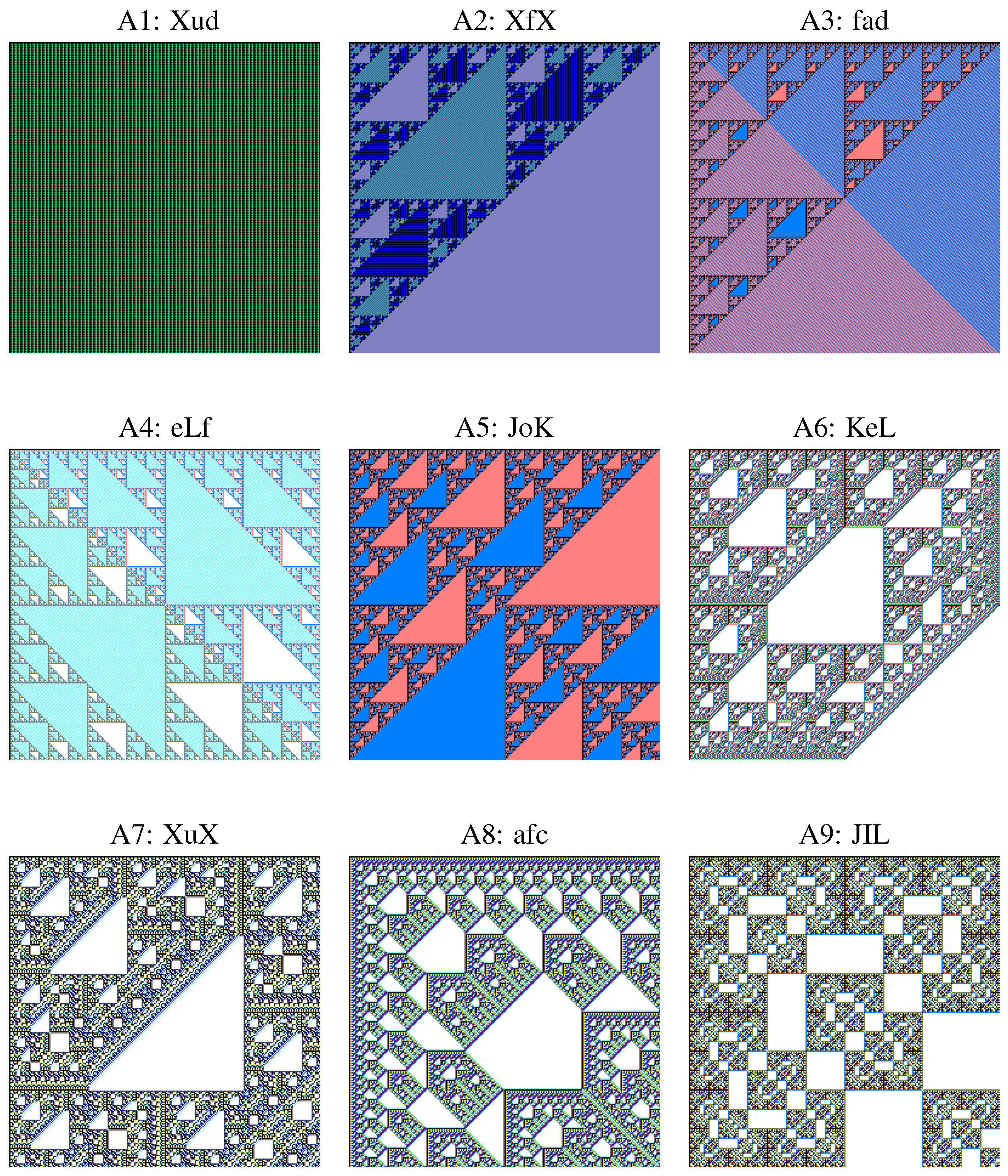
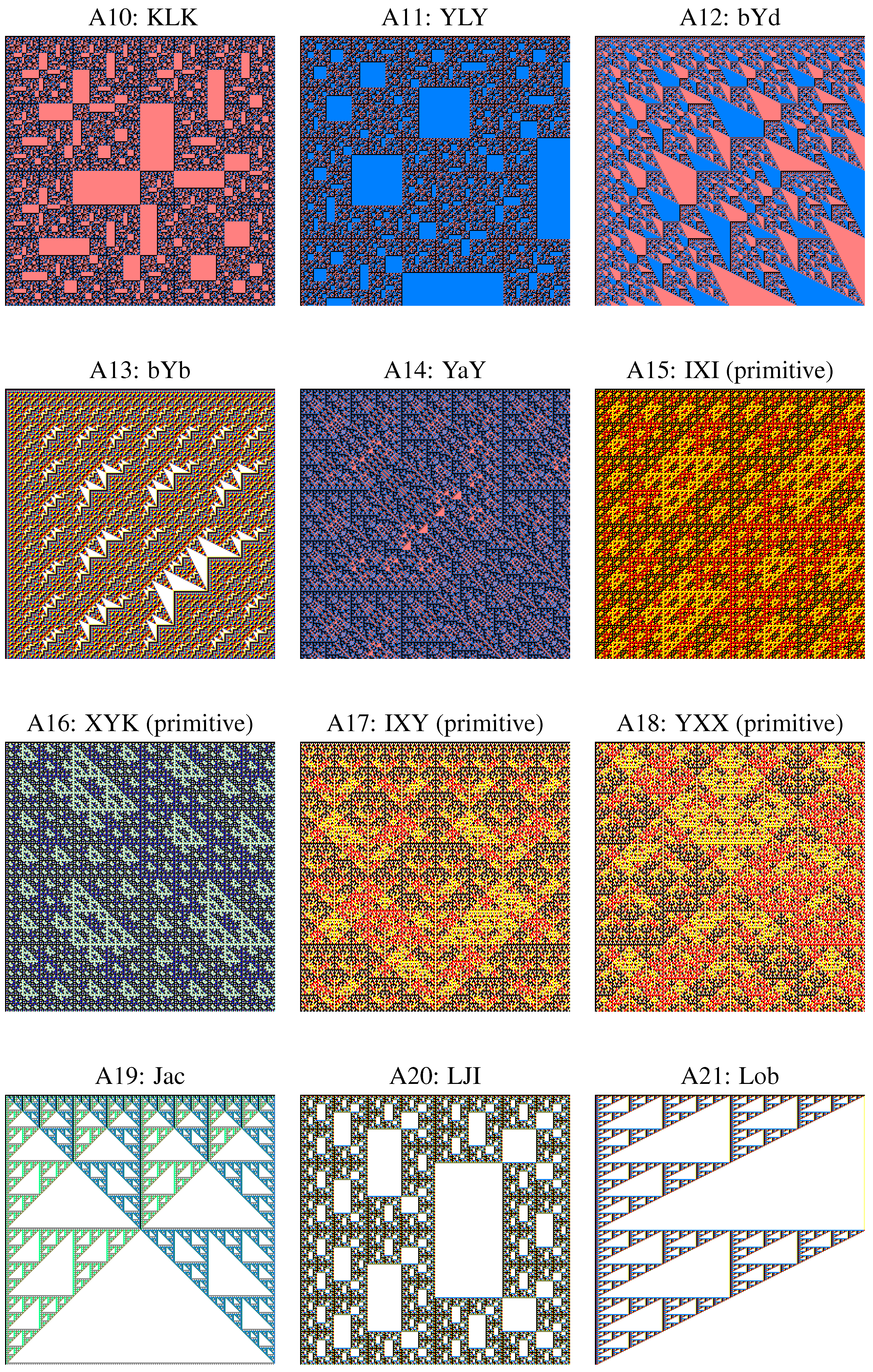
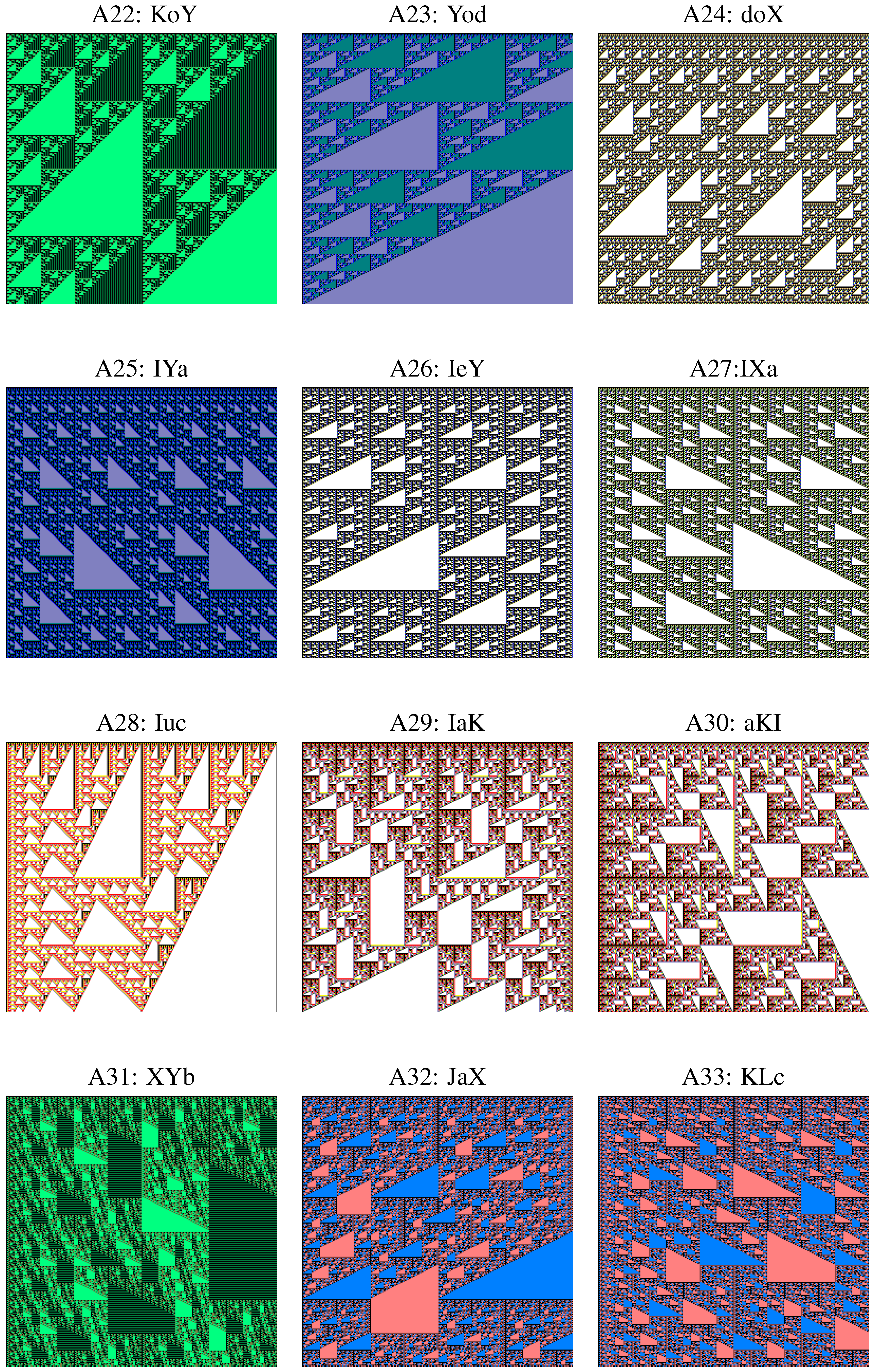
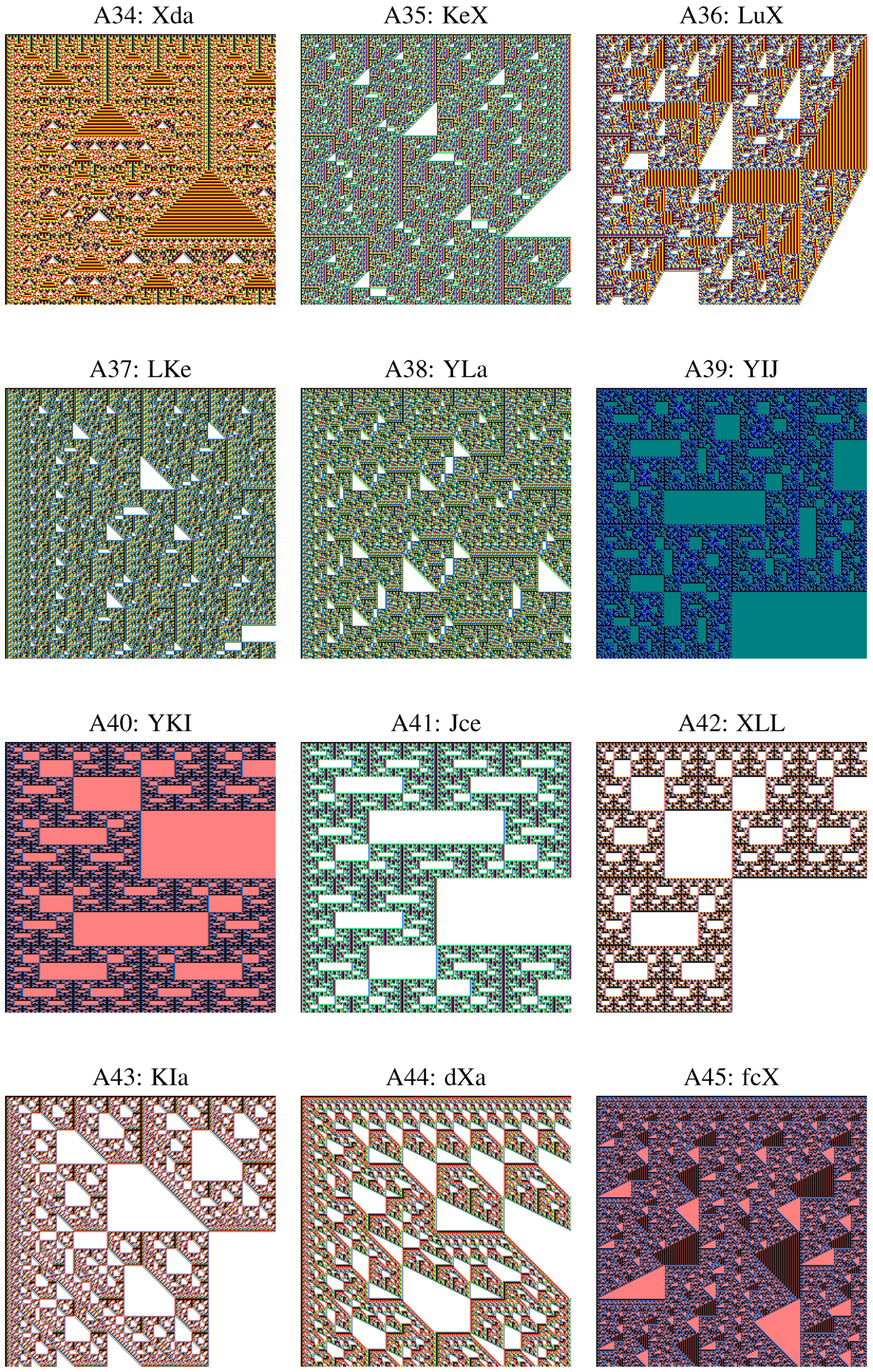
The notion of geometric content that will be defined in this section is based on the following observation: Let a be a double sequence produced by a system of substitutions, of some type $x\to sx$, and let $S_n$ be the $x{s}^{n-1}\times x{s}^{n-1}$ left upper minors defined in the Section 3. Every matrix $S_n$ is graphically represented in the unit square $[0,1]\times [0,1]$: one considers a partition of the unit square in $x{s}^{n-1}\times x{s}^{n-1}$ many equal squares and a set of colors (which is a bijective image of the set) A. One colors the square $s_{ij}$ in the color $S_n(i,j)$. Let us call $G_n$ the graphic obtained. Looking at the sequence of graphics $\left(G_n\right)$ one gets the feeling to see a sequence of images representing the same object with increasing resolution. This justifies the use of the notion of limit of a sequence of sets according to the Hausdorff metric space of compact subsets of ${\mathbb{R}}^2$, as we already have done in [1,3,5]. The problem in doing so is how to define the sequence of converging sets, if one has an arbitrary set of colors, and not only two colors, as in the classical examples of the Sierpinski Gasket, defined by the author in [3] in the form of Pascal’s Triangle mod 2 $({\mathbb{F}}_2,x+z,1)$ or of the Sierpinski Carpet, defined by the author in [3] in the form $({\mathbb{F}}_3,x+y+z,1)$. In this article the author declared those squares $s_{ij}$ corresponding to elements which were $\ne 0$ as belonging to the compact to define. The same was done by the author also in [1], but the convergence had to be proved ad hoc, because the double sequence studied in [1] was already not a tensor product of matrices anymore, like in [3], but the result of an expansive substitution of type $2\to 4$.

If double sequences have the same geometric content, we say that they belong to the same geometric type. At the end of this section we will also give some examples to illustrate the variability inside a geometric type.

Definition 5.1

Let a be a double sequence, M be a $m\times m$ matrix occurring in a in some m-position, and $M^{\prime }$ be another occurrence of M in a in m-position. $M^{\prime }$ is called an m-translation of M. One observes that $M^{\prime }$ and M are identic or disjoint.

Definition 5.2

Let a be a double sequence produced by a system of substitutions $\mathsf{\Sigma }$.

A periodic domain in a is a sequence $\left(U_i\right)$, such that:

• there exist an $m\times m$ matrix M occurring in m-position in a,
• for all i, $U_i$ is a connected union of m-translations of M,
• for all i, $\mathsf{\Sigma }\left(U_i\right)\subseteq U_{i+1}$.

The case of constant sequences $\left(U_i\right)$ with all $U_i=U$ unbounded is not excluded.

We say that a system of substitutions $\mathsf{\Sigma }$ contains periodic domains if the generated sequence a contains periodic domains.

Definition 5.3

Let $\mathsf{\Sigma }$ be a system of substitutions with scaling factor s such that for its skeleton $\sigma =(N,N,\mathcal{Z},1,\sigma )$ there is at least one $m\in N$ with the property that:

$$\sigma \left(m\right)=\left(\begin{array}{cccc}m& m& \cdots & m\\ m& m& \cdots & m\\ ⋮& ⋮& \ddots & ⋮\\ m& m& \cdots & m\end{array}\right)$$

If such a minor m does exist, we call it a repetitive minor. If a double sequence a is generated by a system of substitutions with repetitive minors, then a contains periodic domains.

Definition 5.4

Let a be a double sequence of substitution containing periodic domains and let $\mathsf{\Sigma }$ be a system of substitutions of type $x\to sx$ producing a.

If for every periodic domain in a, its constitutive minor is a repetitive minor in $\mathsf{\Sigma }$, one says that $\mathsf{\Sigma }$ explicitly generates all periodic domains of a.

Let $R\subset N$ be the set of repetitive minors in a substitution system $\mathsf{\Sigma }$ that explicitly generates all periodic domains of a. Let b be the double sequence defined by the skeleton $\sigma$.

For all $n\in \mathbb{N}$ we construct a plane compact set $G_n$ as follows: The unit square $[0,1]\times [0,1]$ is partitioned in $s^n\times s^n$ many equal squares $s_{i,j}$. Now we define $G_n$:

$$G_n:=\bigcup _{\{0\le i,j<s^{n-1}|b(i,j)\in N\backslash R\}}{s}_{ij}$$

Lemma 5.5

If a is a double sequence of substitution containing periodic domains then the sequence of sets $\left(G_n\right)$ converges according to the Hausdorff metric between compact subsets of ${\mathbb{R}}^2$. In this case, the limit $G=lim{G}_n$ is called the geometric content of the double sequence a.

Proof: 

First of all we observe that $G_{n+1}\subset G_n$. Indeed, if $s_{ij}\subset G_n$, the grid partition defining $G_{n+1}$ cuts $s_{ij}$ in $s^2$ many squares, and some of them might not be in $G_{n+1}$. If $s_{ij}\not\subset G_n$, then $s_{ij}\cap G_n=\varnothing$ and so $s_{ij}\cap G_{n+1}=\varnothing$.

Let $d(·,·)$ be the Hausdorff distance for compact plane sets. Recall that $s\ge 2$. One has:

$$d(G_n,G_{n+k})\le d(G_n,G_{n+1})+d(G_{n+1},G_{n+2})+\cdots +d(G_{n+k-1},G_{n+k})\le$$

$$\le s^{-n}(1+s^{-1}+\cdots +s^{-k})<2s^{-n}$$

So $\left(G_n\right)$ is a Cauchy sequence in a complete metric space. Consequently there exists $\underset{n\to \infty }{lim}{G}_n:=G$ and $G={\displaystyle \bigcap _{n\ge 1}}{G}_n\ne \varnothing$.  □

Definition 5.6

Because we do not want to make a difference between the double sequence generated by $ABC$ and $CBA$ (both seen as triples of elements of $M_2\left({\mathbb{F}}_2\right)$) with constant border $=I$, we define:

$$\mathrm{ABC}:=\widehat{ABC}\cup \widehat{CBA}$$

Every set ABC, seen as set of recurrent double sequences, is closed under conjugation and under reflection across the first diagonal of a recurrent double sequence. Such sets, which are mirrored classes of conjugation, will be frequently simply called classes, the distinction being made by notation. Let T be the set of all classes ABC.

Definition 5.7

We define the set of exceptional classes of recurrent double sequences:

$$E=\{\mathrm{IXI},\mathrm{JKL},\mathrm{XJY},\mathrm{XXX},\mathrm{JXY},\mathrm{IIX},\mathrm{IXY},\mathrm{XXY}\}$$

These classes will be classified in the types A15, A16, A17 and A18.

Lemma 5.8

All recurrent double sequences that belong to the classes ABC $\in T\backslash E$ have periodic domains.

Proof: 

We must define another set of less exceptional classes, called F. This definition is most easily done using the forwarded list to be found in the Section 7. In this list the so-called geometric types are given as union as different classes of conjugation, which are grouped in classes of isomorphism of least compatible skeletons. The set F lies completely in $T\backslash E$ and consists of the double sequences listed below. Every set in the list contains sequences with the same skeleton for the smallest substitution type admitted by them (that is, smallest x in $x\to sx$):

{auK}, later in A1, {JXK}, later in A1, {aaL, aeI, aIe, aLa, IIJ, IJI, JJJ}, later in A1, {abX, azY}, later in A1, {aeX, auY, ooX, uaX, udY}, later in A1, {JKX}, later in A1, {JKY}, later in A1, {XIY, XYX}, later in A1, {XoX}, later in A2, {aYc}, later in D73, {oXo, uIv}, later in D73, {oIX}, later in D74, {uJe}, later in E84, {uJf}, later in E84.

For double sequences in $(T\backslash E)\backslash F$: the systems of substitutions of type $x\to sx$ given in Section 7 explicitly generate at least one periodic domain in the corresponding double sequence. Consequently, all these sequences contain periodic domains.

The classes in F have a more special behavior, because they do not contain repetitive minors in the smallest system of substitution generating them. We have found for them other systems of substitution that explicitly have repetitive minors. We do not display here the whole list of results, but we exemplify with a class for every of the skeletons given above. We emphasize that it is not sufficient to check only a class for every skeleton because the appropriate system of substitutions we are looking for is not always a multiple of the smallest system of substitutions. For counterexamples, see uJe and uJf. Here are the appropriate substitution types for:

auK: $4\to 8$, with 2 rules, JXK: $4\to 8$, with 1 rule, JJJ: $2\to 4$, with 1 rule, abX: $6\to 12$, with 2 rules, aeX: $3\to 6$, with 2 rules, JKX: $12\to 24$, with 1 rule, JKY: $6\to 12$, with 1 rule, XIY: $3\to 6$, with 1 rule, XoX: $6\to 12$, with 88 rules, aYc: $3\to 6$, with 3 rules, oIX: $6\to 12$, with 88 rules, uJe: $4\to 8$, with 4 rules, uJf: $4\to 8$, with 4 rules.  □

Examples: Now we show some examples concerning the variability inside a geometric type. The images used to figure left upper minors of recurrent double sequences are pixel-wise computed using a fixed correspondence between the finite set A and a set of colors. For $A=M_2\left({\mathbb{F}}_2\right)$ we have fixed 16 colors, with o represented by white. We do not find important to give the complete list of colors, but we recall that the borders are constant and equal with I.

The first three examples have the same geometric content, so they belong to the same type, which will be called A2.

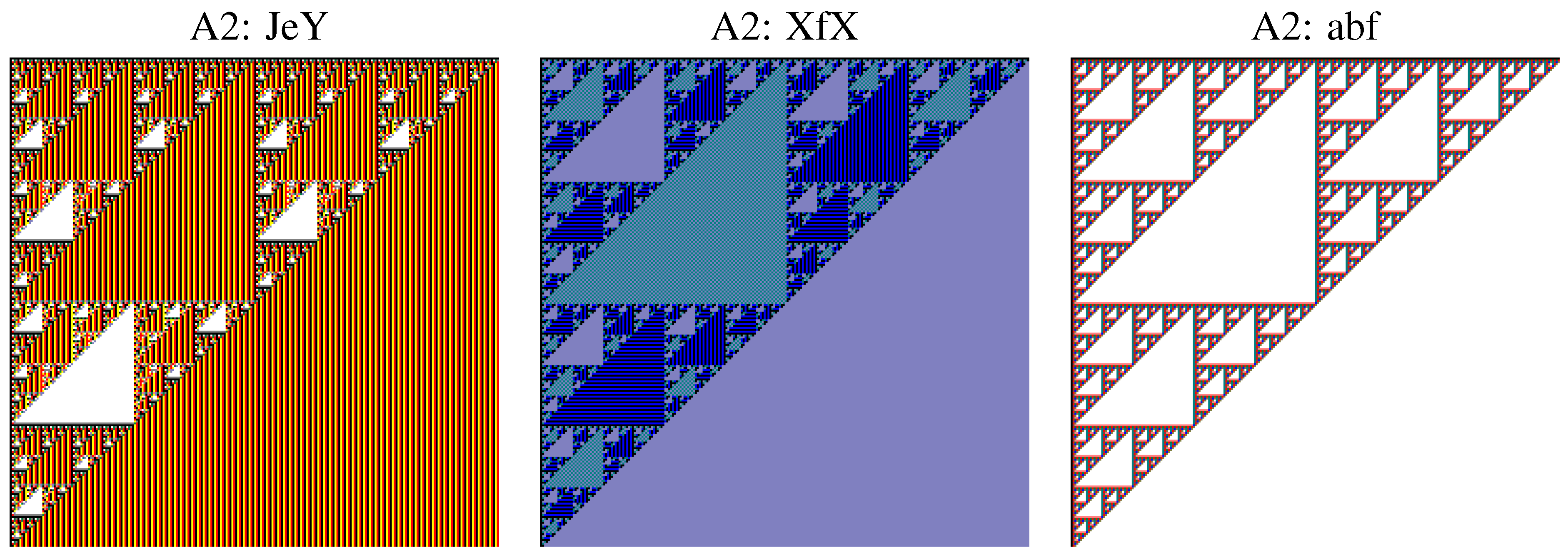
The other examples given here illustrate a standard phenomenon: Many types have some monochromatic and some dichromatic versions. A dichromatic version must be not realized by homogenous domains; there might also be more complicated tissues.

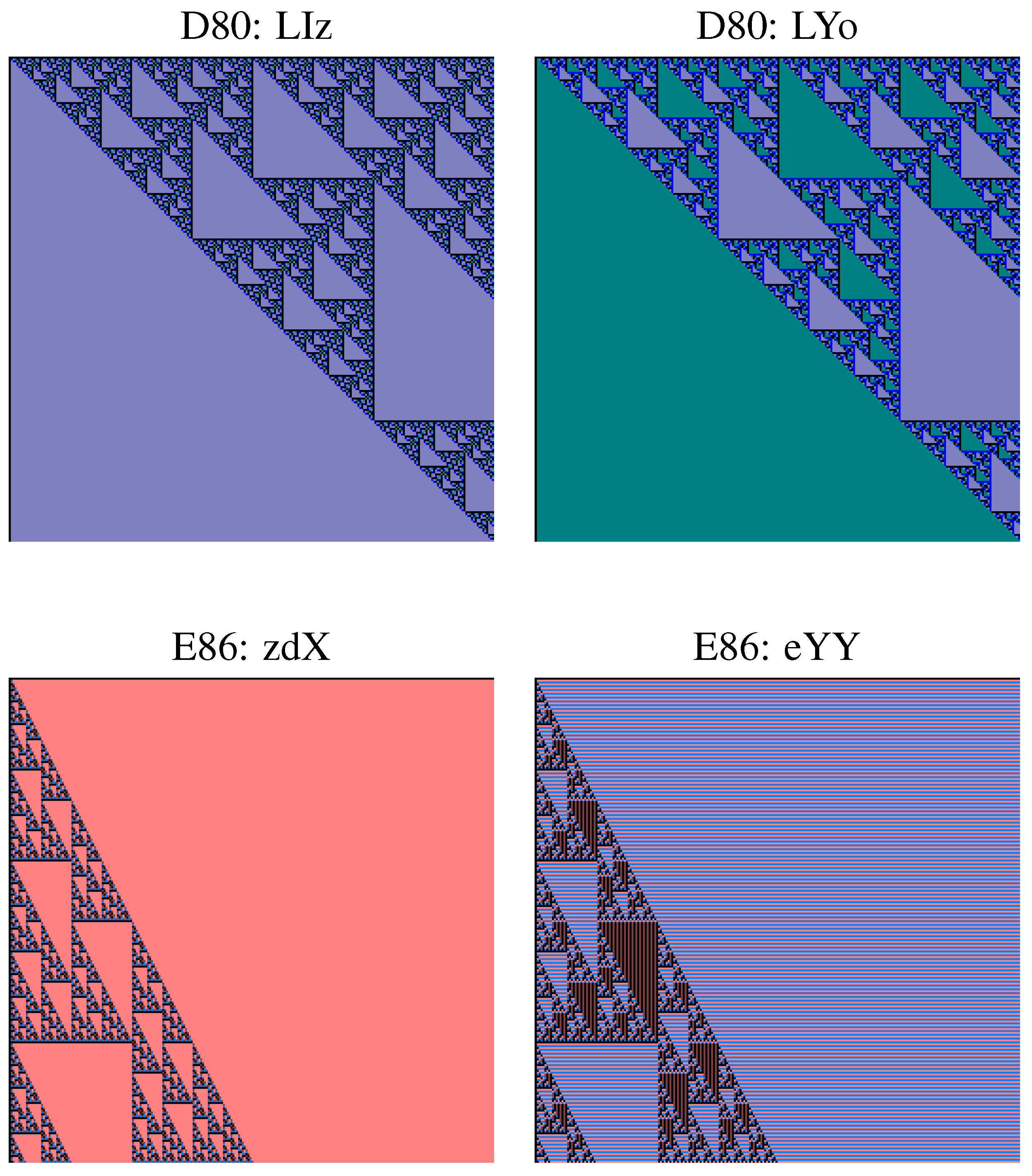
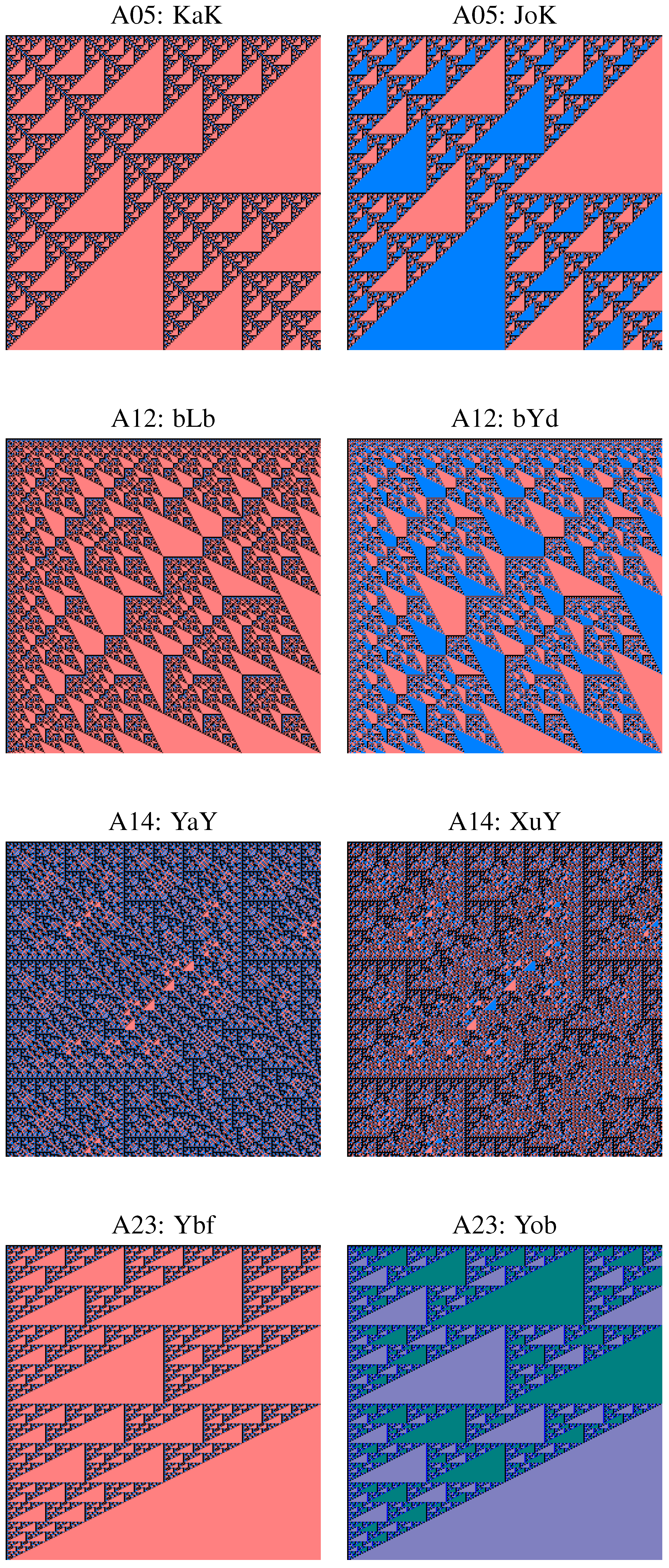
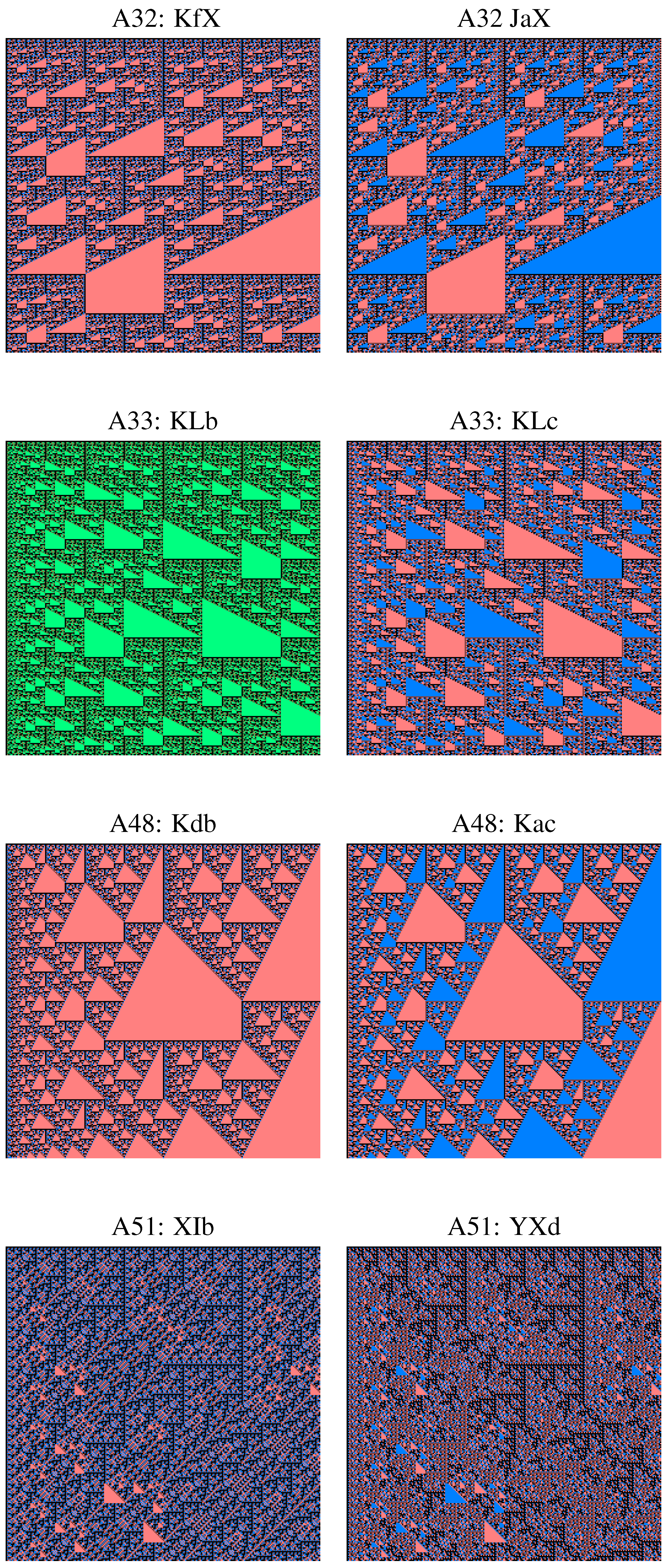
6. Primitive Double Sequences

Now we move on to discuss the classes composing the set E. Their behavior is best exemplified by the double sequence defined by the triple $IXI$ with constant initial condition I. This double sequence is generated by a system of substitutions of type $1\to 2$ with three rules. For this substitution type, double sequences are identical with their skeletons. The minors are $X_1=I$, $X_2=X$, $X_3=Y$, and the set of substitution rules $\mathsf{\Sigma }=\sigma$ is the following:

$$X_1⇝\left(\begin{array}{cc}{X}_1& X_1\\ X_1& X_2\end{array}\right)X_2⇝\left(\begin{array}{cc}{X}_3& X_3\\ X_3& X_1\end{array}\right)X_3⇝\left(\begin{array}{cc}{X}_2& X_2\\ X_2& X_3\end{array}\right)$$

This recurrent double sequence does not contain periodic domains.

Definition 6.1

A system of substitutions $\mathsf{\Sigma }$ with expansion factor s is called primitive if for its skeleton $\sigma =(N,N,\mathcal{Z},1,\sigma )$ the following holds: for every $n\in N$, in the double sequence generated by the system of substitutions ${\sigma }_n=(N,N,\mathcal{Z},n,\sigma )$, which has n as a starting symbol, all elements of N really occurs.

This condition is clearly equivalent with the one that all minors in N do really occur in the double sequence generated by $\sigma ={\sigma }_1$ and that 1 does occur (infinitely often) in the sequences generated by the ${\sigma }_i$, for all i.

If a double sequence a is generated by a primitive system of substitutions $\mathsf{\Sigma }$, we say that a is primitive.

The author thanks Dr. Dirk Frettlöh for informing him about this notion [22]. Over incidence matrices, there is also a historical interpretation of primitivity that reflects in the properties of real matrices with non-negative coefficients, having at least one power with strictly positive coefficients, as in the work of Perron [23]. The most simple example of primitive substitution is maybe the Thue–Morse sequence described in [7,8,9], which is a one-dimensional sequence defined by the expansive substitution rules $0\to 01$ and $1\to 10$ with starting symbol 1. The recurrent double sequence $(M_2\left({\mathbb{F}}_2\right),IXI,I)$, which can be alternatively defined by the three-rule expansive substitution given above, is also primitive.

Definition 6.2

If a double sequence a is generated by a system of substitutions $\mathsf{\Sigma }$ of type $x\to sx$, then a system of substitutions ${\mathsf{\Sigma }}^{\prime }$ of type $kx\to s^{m}kx$ generating a is uniquely determined by $\mathsf{\Sigma }$, k and m and is called a multiple of $\mathsf{\Sigma }$.

We make the following convention: the multiple ${\mathsf{\Sigma }}^{\prime }$ contains in its description only those $kx\times kx$ minors that really occur in a.

Lemma 6.3

If Σ is a primitive system of substitutions then all multiples of Σ are primitive systems of substitution.

Proof: 

Suppose that $\mathsf{\Sigma }$ is of type $x\to sx$ and we are looking at a multiple ${\mathsf{\Sigma }}^{\prime }$ of type $kx\to s^{m}kx$. Minors of ${\mathsf{\Sigma }}^{\prime }$ have block-wise representations given by $k\times k$ $\mathsf{\Sigma }$-minors. Let $X_1$ and $X_1^{\prime }$ be the starting minors corresponding to $\mathsf{\Sigma }$ and ${\mathsf{\Sigma }}^{\prime }$. In particular $X_1$ is the left upper sub-minor of $X_1^{\prime }$. Let $X^{\prime }$ be some minor occurring in a in $kx$-position, and let ${{\mathsf{\Sigma }}^{\prime }}^n\left(X^{\prime }\right)$ be its sequence of successive substitutions. In this sequence there is an element Y containing $X_1$ in some x-position, hence some ${{\mathsf{\Sigma }}^{\prime }}^u\left(Y\right)$ contains a starting sub-minor of a which is big enough to contain the whole $X_1^{\prime }$ inside.  □

Definition 6.4

A double sequence is called periodic if it consists of the infinite repetition of some $k\times k$ minor X. In other words, there is a block-wise representation in $k\times k$ minors $\left(A_{ij}\right)$ such that for all $i,j$ one has $A_{ij}=X$.

Lemma 6.5

If a primitive double sequence a contains periodic domains, it is periodic.

Proof: 

Let ${\mathsf{\Sigma }}_1$ be a system of substitution containing periodic domains that generates a and ${\mathsf{\Sigma }}_2$ be a primitive system of substitutions, also generating a. Let ${\mathsf{\Sigma }}_3$ be a common multiple of ${\mathsf{\Sigma }}_1$ and ${\mathsf{\Sigma }}_2$. On one hand ${\mathsf{\Sigma }}_3$ is primitive, on the other hand the double sequence a contains arbitrarily big periodic domains. Inside such a (big enough) periodic domain one finds the starting symbol $X_1$ of ${\mathsf{\Sigma }}_3$ as left upper minor of an arbitrarily big copy of a starting minor. Hence, arbitrarily big starting minors are periodic, so the whole double sequence is periodic.  □

Lemma 6.6

All the eight classes composing the set E consist of primitive non-periodic double sequences.

Proof: 

By checking the smallest systems of substitution generating the double sequences, as follows: for IXI of type $1\to 2$ with 3 rules, for IIX of type $2\to 4$ with 9 rules, for IXY of type $2\to 4$ with 12 rules, for JKL of type $2\to 8$ with 12 rules, for JXY of type $2\to 8$ with 16 rules, for $XJY$ of type $2\to 4$ with 21 rules, for XXX of type $2\to 4$ with 21 rules and for XXY of type $2\to 4$ with 36 rules. The graphs of the shortest way to 1 if starting from arbitrary $i\in N$ are quite various. If for IXI all the graph is $3⇝2⇝1$, and for JKL the graph consists of all the directed edges $i⇝1$ for all $i\in N\backslash \left\{1\right\}$, in the other cases we meet more complicated graphs.  □

The next Theorem collects together the conclusions of the last two sections:

Theorem 6.7

The recurrent double sequences that belong to the classes ABC $\in T$ have periodic domains if and only if they do not belong to E.

For the classification of the elements of E the author used as criteria only the behavior concerning the symmetries, not only for the sequences themselves but also for their projections, where the word “projection” has the sense defined in the Section 2. Their classification in the geometric types A15, A16, A17 and A18 remains more or less arbitrary. To find a sound notion of geometric content for primitive double sequences seems to remain as a difficult problem.

7. Classification

Let us sum up the relations between recurrent double sequences defined here so far. From finer to coarser we have: class (mirrored class of conjugation), the isomorphism, the same skeleton, and the same geometric content (geometric type).

same class ≺ isomorphic ≺ same skeleton ≺ same geometric type

Our classification of linear double sequences over $M_2\left({\mathbb{F}}_2\right)$ with constant border $=I$ clears the relationships between the different double sequences according to the criteria explained above. A general conclusion can be summed up in the following statement:

Theorem 7.1

The following statements hold:

• Two linear recurrent double sequences over $M_2\left({\mathbb{F}}_2\right)$ with constant border $=I$ are isomorphic if and only if they belong to the same class (mirrored class of conjugation) or are both constant.
• There exist non-isomorphic recurrent double sequences having the same skeleton.
• There exist recurrent double sequences in same geometric type, whose skeletons have the same substitution type $x\to sx$ and the same number of rules, but who have however different skeletons.
• Many of the 90 geometric types contain double sequences with different types of substitution.

Now we are ready to present the classification with details.

Conventions and notations: The notation $Pn$ for the geometric types consist of a prefix P and a number n.

The number n runs from 1 to 90 and is sufficient to determine the type.

The prefix P runs from A to F and encodes only some geometric information, which is defined as follows:

Consider a plane square $\alpha \beta \gamma \delta$. Let $ϵ$ denote the middle of the segment $\beta \gamma$ and let $\eta$ denote the middle of the segment $\gamma \delta$. The point $\alpha$ should be figured as left-upper vertex. Recall that $S_n$ is the $s^n\times s^n$ initial square of the recurrent double sequence S and ${\pi }_n$ is the canonical projection of $S_n$ on the unit square. We consider all the half-lines $\left[\alpha {\pi }_n\left(a(i,j)\right)\right)$, where $a(i,j)$ does not belong to a periodic domain of S.

Let $R_n$ be the union of those half-lines and let $R=R\left(S\right)$ be the topological closure of the Hausdorff limit $lim{R}_n$ in the unit square.

Then the prefixes are:

• A, if $R\left(S\right)\in \{\varnothing ,\alpha \beta ,\alpha \gamma ,\alpha \beta \cup \alpha \gamma ,\alpha \beta \gamma \delta \}$. (51 types)
• B, if $R\left(S\right)\in \{\alpha ϵ\gamma \delta ,\alpha \eta \gamma \beta \}$. (17 types)
• C, if $R\left(S\right)=\alpha ϵ\gamma \eta$. (4 types)
• D, if $R\left(S\right)\in \{\alpha \beta \gamma ,\alpha \delta \gamma \}$. (11 types)
• E, if $R\left(S\right)\in \{\alpha ϵ,\alpha \eta ,\alpha \beta ϵ,\alpha \delta \eta \}$. (4 types)
• F, if $R\left(S\right)\in \{\alpha \gamma \eta ,\alpha \gamma ϵ\}$. (3 types)

The author did not overcome the tentation to give names for the types. The names are a very unessential information: the readers who do not like geometric types to have their own names should just skip them.

Other syntactic rules and conventions are the following:

• We denote with $d_1$ the symmetry around the diagonal $\alpha \gamma$, with $d_2$ the symmetry around the diagonal $\beta \delta$ and with m the median symmetry. When we say that a geometric type fulfills some symmetry, we mean that the geometric content, as Hausdorff limit, does it.
• We denote by t the fact that a half limit is isometric with the other half by translation. The absence of symmetry is abbreviated $ns$.
• We describe a geometric type in the following way:
  number name, symmetry, number of elements, number of classes.
• This line is always followed by the list of skeletons occurring in the type, each of them given together with the list of its own classes.
• If there are different skeletons in the same geometric type and if they have the same type of substitution and the same number of rules, then those skeletons are numbered like “Skeleton 1”, “Skeleton 2”, etc.
• Every name of a class is followed by its number of elements.

A1 Homogenous, $d_1$, 522 double sequences + 256 constant double sequences, 58 classes + 34 classes producing constant double sequences. The non-constant double sequences are given here explicitly:

2 → 4, 4 rules: Skeleton 1: aaa 6, aab 12, aae 12, aba 6, aea 6, oao 6, oaz 12, ooa 12, ooo 1, oou 6, oua 12, oud 12, ouo 3, ouu 6, uaz 12, udc 12, udu 6, uoa 12, uod 12, uou 3, uua 12, uud 12, uuu 3. Skeleton 2: auK 12.

2 → 4, 2 rules: Skeleton 1: aaJ 12, abI 12, aoc 12, aud 12, azK 12, oac 12, ooJ 6, ouI 6, uda 12, udK 12, uoI 6, uuL 6. Skeleton 2: JXK 12.

1 → 2, 2 rules: aaL 12, aeI 12, aIe 6, aLa 6, IIJ 6, IJI 3, JJJ 3.

3 → 6, 3 rules: abX 12, azY 12.

2 → 4, 6 rules: Skeleton 1: aeX 12, auY 12, ooX 4, uaX 12, udY 12. Skeleton 2: JKX 12.

2 → 4, 3 rules: Skeleton 1: JKY 12. Skeleton 2: uaK 12.

3 → 6, 5 rules: uab 12.

2 → 4, 5 rules: uau 6.

2 → 4, 9 rules: XIY 2, XYX 2.

A2 Pascal Triangle, $d_1$, 262 double sequences, 34 classes.

2 → 4, 5 rules: Skeleton 1: aaK 12, azI 12. Skeleton 2: aoa 6.

2 → 4, 7 rules: abf 12, aob 6, aoe 6, aua 6, aue 6, aza 6, azb 6.

1 → 2, 2 rules: ada 6, ade 12, afa 6, aoI 12, aoL 12, auI 12, auL 12, IaI 6, IaJ 12, IoI 1, JaJ 6.

2 → 4, 6 rules: aoJ 12.

3 → 6, 48 rules: azJ 12.

2 → 4, 4 rules: IaL 12, IoJ 6, IuL 6.

2 → 4, 16 rules: IoX 4.

1 → 2, 3 rules: IuI 3.

2 → 4, 8 rules: JcJ 6, JoJ 3, JzJ 3.

6 → 12, 128 rules: JeY 12.

2 → 4, 28 rules: XaX 6.

2 → 4, 51 rules: XoX 2.

A3 Pascal Triangle and Diagonal, $d_1$, 24 double sequences, 3 classes.

2 → 4, 11 rules: aca 6.

3 → 6, 181 rules: acb 12.

2 → 4, 19 rules: avd 6.

A4 Hour Glasses, $d_1$, $d_2$, 48 double sequences, 5 classes. See [1].

2 → 4, 34 rules: aIc 12, aJc 12, aJd 12, aYa 6.

2 → 4, 11 rules: aId 6.

A5 Double Wave Pascal, $d_1$, 12 double sequences, 2 classes.

2 → 4, 7 rules: JeJ 6.

2 → 4, 10 rules: JoK 6.

A6 Diamond, $d_1$, 18 double sequences, 2 classes. See [1].

2 → 4, 42 rules: JaL 12, JuJ 6.

A7 Brilliant, $d_1$, 6 double sequences, 1 class.

2 → 4, 56 rules: XuX 6.

A8 Twin Peaks, $d_1$, 18 double sequences, 2 classes. See [1].

2 → 4, 51 rules: acf 12, ava 6.

A9 Open Peano, $d_1$ 12 double sequences, 2 classes. See [6].

2 → 4, 27 rules: JIK 6, JXJ 6.

A10 Swallow, $d_1$, 6 double sequences, 1 class.

2 → 4, 15 rules: JKJ 6.

A11 Squares, $d_1$, 6 double sequences, 1 class.

4 → 8, 59 rules: XJX 6.

A12 Angel, $d_1$, 18 double sequences, 2 classes.

2 → 4, 15 rules: aKa 6.

4 → 8, 30 rules: aXc 12.

A13 Butterfly Families, $d_1$, 12 double sequences, 2 classes.

2 → 4, 41 rules: aKd 6, aXa 6.

A14 Four Stars, $d_1$, 12 double sequences, 2 classes.

2 → 4, 60 rules: XbX 6.

4 → 8, 120 rules: XuY 6.

A15 Trace 1, $d_1$, 16 double sequences, 4 classes. These double sequences are all primitive.

1 → 2, 3 rules: IXI 2.

2 → 8, 12 rules: JKL 6.

2 → 4, 21 rules: XJY 6, XXX 2.

A16 Trace 2, $d_2$, 16 double sequences, 2 classes. These double sequences are all primitive.

2 → 4, 9 rules: IIX 4.

2 → 8, 16 rules: JXY 12.

A17 Trace Median, $ns$, 4 double sequences, 1 class. These double sequences are all primitive.

2 → 4, 12 rules: IXY 4.

A18 Trace Rectangular, $ns$, 4 double sequences, 1 class. These double sequences are all primitive.

2 → 4, 36 rules: XXY 4.

A19 Mirrored Triangle, m, 84 double sequences, 7 classes.

2 → 4, 12 rules: acI 12, afI 12.

2 → 4, 16 rules: acJ 12, adJ 12, adL 12, afL 12.

2 → 4, 7 rules: adI 12.

A20 Mirrored Rectangles, m, 12 double sequences, 1 class.

2 → 4, 10 rules: IJK 12.

A21 Long Triangles I, t, 72 double sequences, 6 classes.

2 → 4, 9 rules: abL 12, aeJ 12, aoK 12.

2 → 4, 5 rules: IuJ 12, JcL 12.

2 → 4, 7 rules: JaK 12.

A22 Shifted Triangles, $ns$, 12 double sequences, 1 class.

2 → 4, 10 rules: JoX 12.

A23 Shifted Long Triangles I, $ns$, 48 double sequences, 4 classes.

4 → 8, 19 rules: abY 12.

2 → 4, 11 rules: aeY 12.

2 → 4, 19 rules: aoX 12.

2 → 4, 8 rules: IuX 12.

A24 Left Meteorites, $ns$, 60 double sequences, 5 classes.

2 → 4, 25 rules: aaX 12.

2 → 4, 16 rules: aoY 12.

2 → 4, 13 rules: IaY 12, JuY 12.

2 → 4, 22 rules: JuX 12.

A25 Right Meteorites, $ns$, 84 double sequences, 7 classes.

2 → 4, 24 rules: Skeleton 1: abe 12, aeb 12, auc 12. Skeleton 2: avc 12.

4 → 8, 8 rules: aJK 12.

2 → 4, 8 rules: aLK 12, aYI 12.

A26 Left Comets, $ns$, 12 double sequences, 1 class.

2 → 4, 9 rules: IaX 12.

A27 Right Comets, $ns$, 12 double sequences, 1 class.

2 → 4, 9 rules: aXI 12.

A28 Pythagoras vs. Pascal, $ns$, 24 double sequences, 2 classes.

2 → 8, 25 rules: adK 12.

2 → 4, 14 rules: avI 12.

A29 Left Broken Arrows, $ns$, 24 double sequences, 2 classes.

2 → 4, 14 rules: IaK 12.

2 → 8, 23 rules: JuL 12.

A30 Right Broken Arrows, $ns$, 24 double sequences, 2 classes.

2 → 4, 16 rules: aKI 12.

2 → 8, 28 rules: aXK 12.

A31 Interrupted I, $ns$, 12 double sequences, 1 class.

4 → 8, 30 rules: aXY 12.

A32 Interrupted Long, $ns$, 24 double sequences, 2 classes.

4 → 8, 56 rules: JaX 12.

2 → 4, 28 rules: JcX 12.

A33 Interrupted Short, $ns$, 24 double sequences, 2 classes.

4 → 8, 30 rules: aKJ 12,

2 → 4, 15 rules: aKL 12,

A34 Lamps, $ns$, 24 double sequences, 2 classes.

2 → 4, 112 rules: adX 12, avY 12.

A35 Half Lamps, $ns$, 24 double sequences, 2 classes.

2 → 4, 52 rules: JaY 12, JcY 12.

A36 High Half Lamps I, $ns$, 12 double sequences, 1 class.

2 → 4, 104 rules: JzX 12.

A37 Small Half Lamps, $ns$, 24 double sequences, 2 classes.

2 → 4, 52 rules: aJL 12, aLJ 12.

A38 Pairs Small Half Lamps, $ns$, 24 double sequences, 2 classes.

2 → 4, 60 rules: aJY 12, aLY 12.

A39 Balks, $ns$ 12 double sequences, 1 class.

2 → 4, 30 rules: JIX 12.

A40 Shifted Balks Generation, $ns$, 60 double sequences, 5 classes.

2 → 4, 19 rules: aaY 12.

2 → 4, 28 rules: auX 12, azX 12.

2 → 4, 16 rules: IJX 12, JXX 12.

A41 Shifted Balks Decay, $ns$, 72 double sequences, 6 classes.

2 → 4, 27 rules: abK 12, aeK 12, auJ 12, azL 12.

2 → 4, 8 rules: Skeleton 1: IXJ 12. Skeleton 2: JJK 12.

A42 Shifted Rectangles, $ns$, 12 double sequences, 1 classes.

2 → 4, 20 rules: JJX 12.

A43 Shifted Diamonds, $ns$, 36 double sequences, 3 classes.

2 → 4, 51 rules: aIK 12, aYJ 12, aYL 12.

A44 Cancer, $ns$, 36 double sequences, 3 classes.

2 → 4, 52 rules: Skeleton 1: aJe 12, Skeleton 2: aKb 12, aXd 12,

A45 Dragon I, $ns$, 24 double sequences, 2 classes.

4 → 8, 32 rules: acX 12.

2 → 4, 32 rules: afX 12.

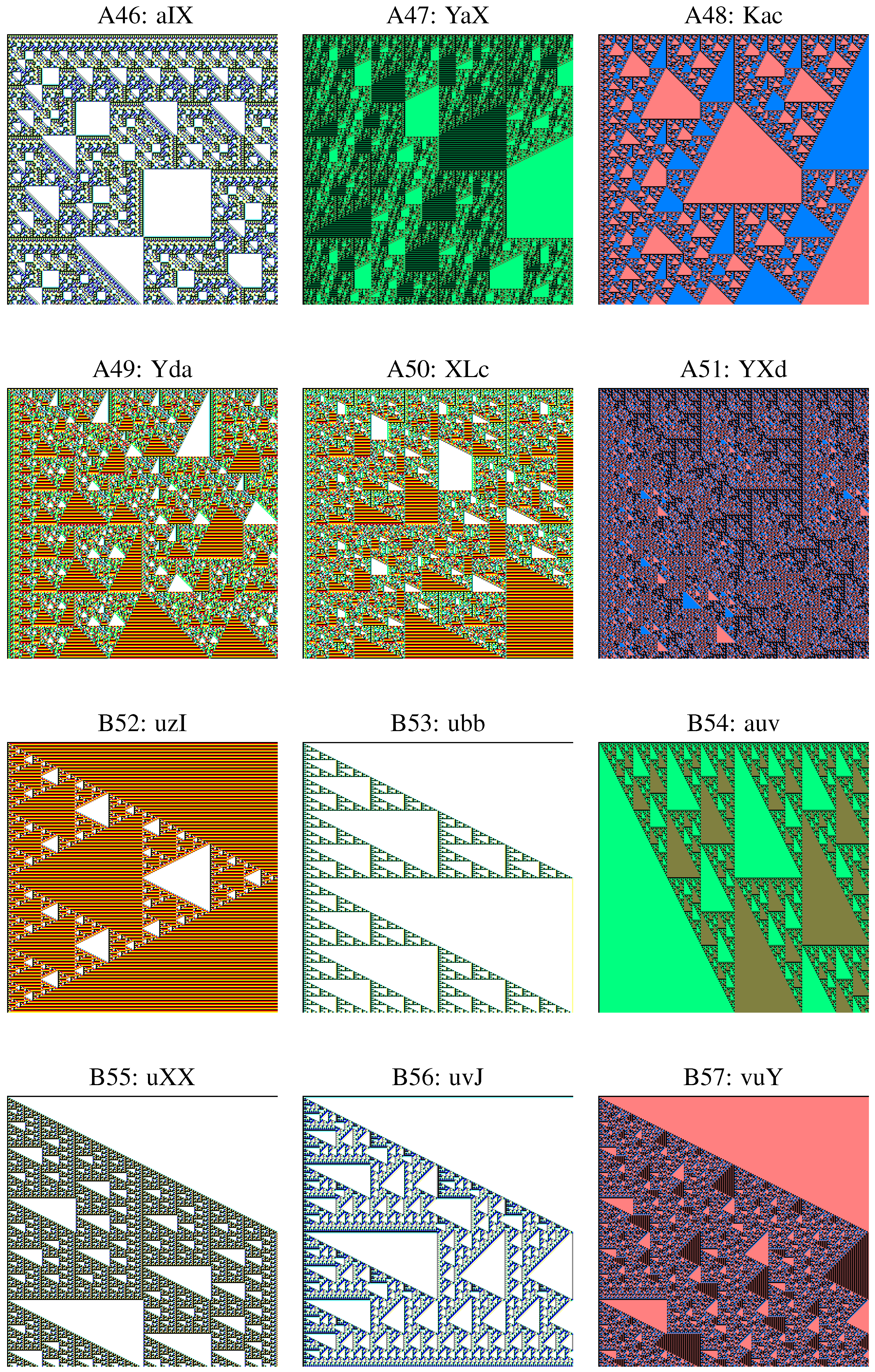
A46 Fish, $ns$, 12 double sequences, 1 class.

2 → 4, 56 rules: aIX 12.

A47 Stone Chain, $ns$, 12 double sequences, 1 class.

2 → 4, 58 rules: XaY 12.

A48 Quadrilaterals, $ns$, 36 double sequences, 3 classes.

2 → 4, 15 rules: acL 12.

2 → 4, 30 rules: afJ 12.

4 → 8, 30 rules: avK 12.

A49 Regatta I, $ns$, 12 double sequences, 1 class.

2 → 4, 116 rules: adY 12.

A50 Trapezes, $ns$, 12 double sequences, 1 class.

2 → 4, 112 rules: aKX 12.

A51 Falling Stars, $ns$, 24 double sequences, 2 classes.

2 → 4, 31 rules: aIY 12.

4 → 8, 62 rules: aYX 12.

B52 Isosceles Triangles, m, 12 double sequences, 1 class.

4 → 8, 16 rules: uvI 12.

B53 Long Triangles II, t, 72 double sequences, 6 classes.

4 → 8, 13 rules: ubb 12, uve 12, uvf 12.

4 → 8, 10 rules: uJI 12, uXJ 12, uXK 12.

B54 Shifted Long Triangles II, $ns$, 60 double sequences, 5 classes.

4 → 8, 31 rules: uba 12, uvb 12, uvc 12.

4 → 8, 17 rules: ubf 12.

4 → 8, 8 rules: uXI 12.

B55 Falling Comets, $ns$, 12 double sequences, 1 class.

4 → 8, 17 rules: uXX 12.

B56 Pascal vs. Pythagoras, $ns$, 24 double sequences, 2 classes.

4 → 8, 14 rules: ubI 12.

4 → 16, 25 rules: uvJ 12.

B57 Dragon II, $ns$, 24 double sequences, 2 classes.

4 → 8, 58 rules: uvX 12, uvY 12.

B58 Regatta II, $ns$, 12 double sequences, 1 class.

4 → 8, 116 rules: ubX 12.

B59 Descendant, $ns$, 36 double sequences, 3 classes.

4 → 8, 30 rules: ubc 12, uva 12, uvd 12.

B60 Ascendant, $ns$, 36 double sequences, 3 classes.

4 → 8, 50 rules: ubJ 12, uvL 12.

4 → 8, 25 rules: ubK 12.

B61 High Half Lamps II, $ns$, 12 double sequences, 1 class.

4 → 8, 104 rules: uJL 12.

B62 Skyrockets, $ns$, 24 double sequences, 2 classes.

4 → 8, 28 rules: ubL 12, uvK 12.

B63 Cancer Lamps, $ns$, 36 double sequences, 3 classes.

4 → 8, 51 rules: uJa 12, uJd 12, uXb 12.

B64 Cut Lamps, $ns$, 12 double sequences, 1 class.

4 → 8, 58 rules: uXY 12.

B65 Parallelograms, $ns$, 24 double sequences, 2 classes.

4 → 8, 112 rules: uXa 12, uXf 12.

B66 Interrupted II, $ns$, 24 double sequences, 2 classes.

4 → 8, 106 rules: uJX 12.

4 → 8, 53 rules: uJY 12.

B67 Broken Arrows, $ns$, 24 double sequences, 2 classes.

4 → 8, 37 rules: uJJ 12, uXL 12.

B68 Slim Triangles, $ns$, 24 double sequences, 2 classes.

4 → 8, 108 rules: ubd 12, ube 12.

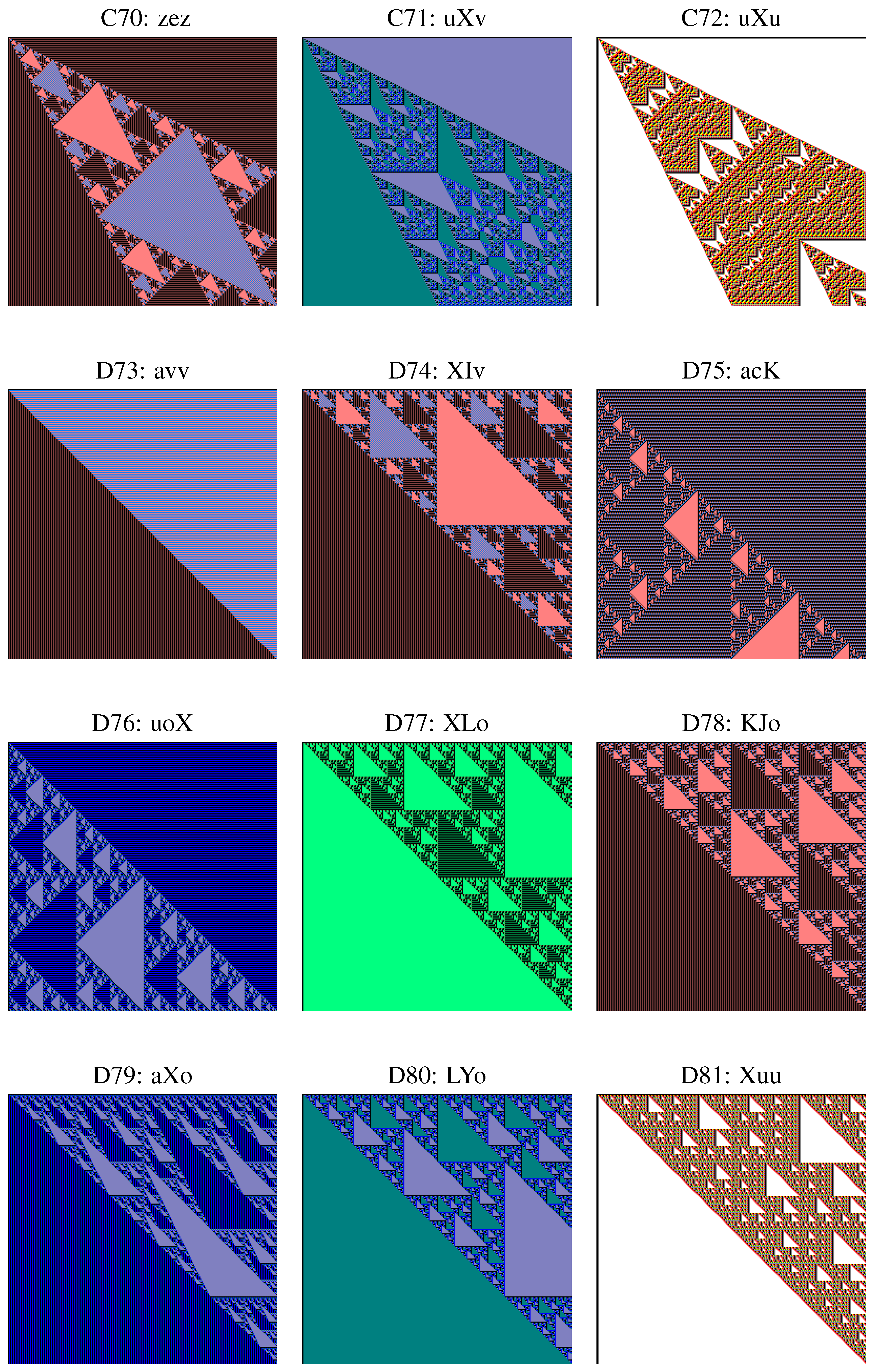
C69 Pascal Slim Cut, $d_1$, 6 double sequences, 1 class.

3 → 6, 32 rules: uvu 6.

C70 Pascal Slim Vertex, $d_1$, 6 double sequences, 1 class.

4 → 8, 32 rules: ubu 6.

C71 Single Butterflies, $d_1$, 18 double sequences, 2 classes.

4 → 8, 43 rules: uJu 6.

4 → 8, 86 rules: uXv 12.

C72 Pairs of Butterflies, $d_1$, 12 double sequences, 2 classes.

4 → 8, 41 rules: uJv 6, uXu 6.

D73 Diagonal, $d_1$, 98 double sequences, 13 classes.

2 → 4, 3 rules: aIb 6, aJa 6, oIu 6, oJo 3, uad 12, uLu 3, oaf 12.

2 → 4, 6 rules: Skeleton 1: aYc 12. Skeleton 2: oau 12, uov 6.

2 → 4, 9 rules: oXo 2, uIv 6.

2 → 4, 5 rules: uub 12.

D74-Pascal Rotated, $d_2$, 560 double sequences, 53 classes.

2 → 4, 6 rules: Skeleton 1: aac 12. Skeleton 2: ave 12.

2 → 4, 4 rules: aad 12, aaf 12, acd 12, adc 12, aII 12, aIJ 12, aJI 12, aJJ 12, aLI 12, oaI 12, oaL 12, oIa 12, oII 2, oJc 12, oJI 6, uaI 12, uaL 12, uIa 12, uII 6, uLa 12, uLI 6.

4 → 8, 6 rules: abc 12, aub 12.

2 → 4, 10 rules: Skeleton 1: abd 12. Skeleton 2: oaJ 12, udL 12.

2 → 4, 8 rules: Skeleton 1: aIL 12, aLL 12, oIJ 6, oJJ 6, uIL 6, uLL 6. Skeleton 2: oJa 12.

2 → 4, 7 rules: oaa 12, oab 12, oae 12, uaa 12, uae 12, udd 12, udf 12, uob 12.

2 → 4, 51 rules: oIX 4.

2 → 4, 16 rules: Skeleton 1: oXI 4. Skeleton 2: uIX 12.

2 → 4, 40 rules: oXX 4, uLX 12.

2 → 4, 5 rules: udI 12, uuJ 12.

2 → 4, 11 rules: uId 12.

3 → 6, 51 rules: uLd 12.

6 → 12, 128 rules: uLJ 12.

D75 Shifted Pascal, $ns$, 72 double sequences, 6 classes.

4 → 8, 12 rules: acK 12.

2 → 4, 12 rules: afK 12, avJ 12, avL 12.

2 → 4, 22 rules: oaK 12.

2 → 4, 14 rules: uoJ 12.

D76 Shifted Double Pascal, $ns$, 48 double sequences, 4 classes.

2 → 4, 14 rules: acY 12, afY 12.

2 → 4, 19 rules: oaX 12.

2 → 4, 11 rules: uoX 12.

D77 Half Shifted Pascal, $ns$, 12 double sequences, 1 class.

4 → 8, 20 rules: oJX 12,

D78 Shifted Triangles Rotated, $ns$, 12 double sequences, 1 class.

4 → 8, 10 rules: oJK 12.

D79 Splits, $ns$, 24 double sequences, 2 classes.

2 → 4, 16 rules: oXa 12.

4 → 8, 16 rules: uLb 12.

D80 Shifted Double Pascal, $ns$, 24 double sequences, 2 classes.

2 → 4, 20 rules: oXJ 12.

2 → 4, 10 rules: uIJ 12.

D81 Comets Up, $ns$, 60 double sequences, 5 classes.

4 → 8, 13 rules: aJX 12.

2 → 4, 13 rules: aLX 12, aYY 12.

2 → 4, 16 rules: oaY 12, uuX 12.

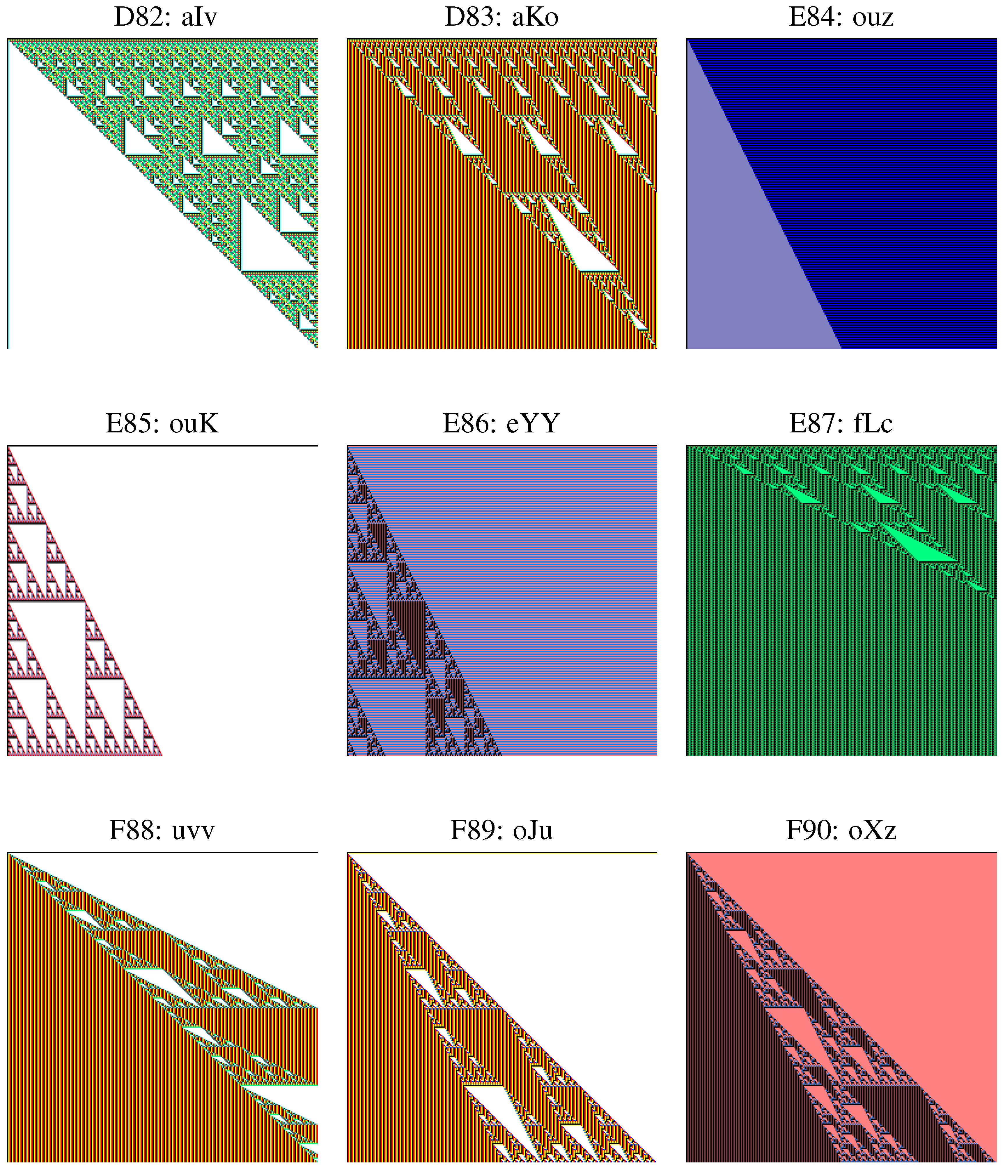
D82 Comets Down, $ns$, 24 double sequences, 2 classes.

2 → 4, 23 rules: oXb 12, uIb 12.

D83 UFOs I, $ns$, 12 double sequences, 1 class.

4 → 8, 28 rules: oJe 12.

E84 Median to Vertex, $ns$, 60 double sequences, 5 classes.

3 → 6, 8 rules: ouv 12.

4 → 8, 8 rules: uav 12.

3 → 6, 9 rules: ubz 12.

3 → 6, 10 rules: uJe 12.

3 → 6, 14 rules: uJf 12.

E85 Single Long Triangle, $ns$, 72 double sequences, 6 classes.

2 → 4, 5 rules: aKK 12, aXL 12.

4 → 8, 5 rules: aXJ 12.

2 → 4, 7 rules: ouJ 12.

2 → 4, 9 rules: uaJ 12, udJ 12.

E86 Shifted Single Long triangle, $ns$, 48 double sequences, 4 classes.

2 → 4, 16 rules: aXX 12.

2 → 4, 19 rules: ouX 12.

2 → 4, 17 rules: uaY 12.

2 → 4, 31 rules: udX 12.

E87 UFOs II, $ns$, 84 double sequences, 7 classes.

4 → 8, 16 rules: Skeleton 1: aJf 12. Skeleton 2: aXb 12.

2 → 4, 16 rules: aKf 12, aXe 12.

2 → 4, 18 rules: oub 12.

2 → 4, 34 rules: uac 12, udb 12.

F88 UFOs III, $ns$, 72 double sequences, 6 classes.

4 → 8, 35 rules: oav 12, uuv 12.

4 → 8, 32 rules: uJb 12, uJc 12, uXd 12, uXe 12.

F89 Shadows, $ns$, 12 double sequences, 1 class.

4 → 8, 28 rules: oJu 12.

F90 Double Shadows, $ns$, 24 double sequences, 2 classes.

4 → 8, 28 rules: Skeleton 1: oXu 12. Skeleton 2: uJz 12.

8. Affine Recurrence Rules and Two Secret Types

Are we really happy with our 256 constant double sequences, which are sometimes produced by quite sophisticated matrix triples? Is it not just a lack of chance that the first generated element $a(1,1)$ was $=I$, so the whole double sequence was condemned to remain constant? What can we do in order to see what we miss? To replace the starting value I with another element of the ring $M_2\left({\mathbb{F}}_2\right)$ does not help us in the given situation, because of the linearity of the recurrence.

Instead, having computed all the double sequences $ABCD$ over $M_2\left({\mathbb{F}}_2\right)$ given by initial conditions $a(i,0)=a(0,j)=I$ and by the recurrence

$$a(i,j)=Aa(i,j-1)+Ba(i-1,j-1)+Ca(i-1,j)+D$$

where $A,B,C,D\in M_2\left({\mathbb{F}}_2\right)$ are fixed, we have found out the following facts:

• All these double sequences are generated by systems of substitutions.
• For non-constant double sequences ABC, adding a constant D in the recurrence does not change the geometric type.
• For most of the triples ABC generating constant double sequences, the various types ABCD generate double sequences in one of the 90 geometric types given above. The geometric type depend only on the triple ABC, and not on the constant $D\in M_2\left({\mathbb{F}}_2\right)\backslash \left\{0\right\}$ that have been added in the recurrence formula.
• There are only two new geometric types revealed in the (formerly) constant double sequences, as follows:
  • A91 Byzantine Mosaics, $d_1$, got for example by all XIXD with $D\in M_2\left({\mathbb{F}}_2\right)\backslash \left\{0\right\}$. These sequences are primitive. All XIXD are of type $2\to 4$ with 12 rules and with the same skeleton for all $D\in M_2\left({\mathbb{F}}_2\right)\backslash \left\{0\right\}$.
  • B92 Double Triangles, $ns$, got for example by ubYD$D\in M_2\left({\mathbb{F}}_2\right)\backslash \left\{0\right\}$. These sequences have periodic domains and a conventional geometric content. All ubYD are of type $4\to 8$ with 12 rules, and have again the same skeleton for all $D\in M_2\left({\mathbb{F}}_2\right)\backslash \left\{0\right\}$.

We do not insist anymore in classifying the affine sequences over $M_2\left({\mathbb{F}}_2\right)$. We hope that this description of the recurrent double sequences in the smallest matrix ring will animate the reader to participate at the inevitable construction of this new theory.

References

- Prunescu, M. Recurrent double sequences that can be generated by context-free substitutions. Fractals 2010, 18, 65–73. [Google Scholar] [CrossRef]
- Prunescu, M. Undecidable properties of recurrent double sequences. Notre Dame J. Formal Logic 2008, 49, 143–151. [Google Scholar] [CrossRef]
- Prunescu, M. Self-similar carpets over finite fields. Eur. J. Combinatorics 2009, 30, 866–878. [Google Scholar] [CrossRef]
- Passoja, D.E.; Lakhtakia, A. Carpets and rugs: An exercise in numbers. Leonardo 1992, 25, 69–71. [Google Scholar] [CrossRef]
- Prunescu, M. Recurrent two-dimensional sequences generated by homomorphisms of finite abelian groups with periodic initial conditions. Preprint 2010. http://home.mathematik.uni-freiburg.de/prunescu/prunescu.html To appear in Fractals.
- Prunescu, M. Counterexample to context-free substitution in recurrent double sequences over finite sets. Preprint 2010. http://home.mathematik.uni-freiburg.de/prunescu/prunescu.html.
- Allouche, J.-P.; Shallit, J. Automatic Sequences-Theory, Applications, Generalizations; Cambridge University Press: Cambridge, UK, 2003. [Google Scholar]
- Allouche, J.-P.; Shallit, J. The Ubiquitous Prouhet-Thue-Morse Sequence; Sequences and their applications (Singapore 1998), springer series discrete mathematics in theoretical computer science; Springer: London, UK, 1999; pp. 1–16. [Google Scholar]
- Muchnik, A.A.; Pritykin, Y.L.; Semenov, A.L. Sequences close to periodic. Russ. Math. Surv. 2009, 64, 805–871. [Google Scholar] [CrossRef]
- Willson, S.J. Cellular automata can generate fractals. Discrete Appl. Math. 1984, 8, 91–99. [Google Scholar] [CrossRef]
- Mandelbrot, B.B. The Fractal Geometry of Nature; W.H. Freeman and Company: San Francisco, CA, USA, 1982. [Google Scholar]
- Kari, J. Theory of cellular automata: A survey. Theor. Comput. Sci. 2005, 334, 3–33. [Google Scholar] [CrossRef]
- Wolfram, S. A New Kind of Science; Wolfram Media: Champaign, IL, USA, 2002. [Google Scholar]
- Penrose, R. Pentaplexity. Math. Intell. 1979, 2, 32–37. [Google Scholar] [CrossRef]
- Wang, H. Proving theorems by pattern recognition. Commun. ACM 1960, 3, 220–234. [Google Scholar] [CrossRef]
- Robinson, R.M. Undecidability and nonperiodicity for tilings of the plane. Invent. Math. 1971, 12, 177–209. [Google Scholar] [CrossRef]
- Grunbaum, B.; Shephard, G.C. Tilings and Patterns; Dover Publications: Mineola, NY, USA, 2011. [Google Scholar]
- Lindenmayer, A.; Prusinkiewicz, P. The Algorithmic Beauty of Plants; Springer Verlag: Berlin, Germany, 1996. [Google Scholar]
- Rozenberg, G.; Salomaa, A. Lindenmayer Systems: Impacts on Theoretical Computer Science, Computer Graphics, and Developmental Biology; Springer Verlag: Berlin, Germany, 1992. [Google Scholar]
- Baake, M.; Moody R., V. (Eds.) Directions in Mathematical Quasicrystals; CRM Monograph Series; AMS: Providence, RI, USA, 2000. [Google Scholar]
- Moody, R.V. The Mathematics of Aperiodic Order. Proceedings of the NATO Advanced Study Institute on Long Range Aperiodic Order; Kluwer Academic Publishers: Norwell, MA, USA, 1997. [Google Scholar]
- Frettlöh, D. Duality of model sets generated by substitution. Rom. J. Pure Appl. Math. 2005, 50, 619–639. [Google Scholar]
- Perron, O. Zur Theorie der matrices. Math. Ann. 1907, 64, 248–263. [Google Scholar] [CrossRef]
© 2011 by the authors; licensee MDPI, Basel, Switzerland. This article is an open access article distributed under the terms and conditions of the Creative Commons Attribution license (http://creativecommons.org/licenses/by/3.0/).
Share and Cite
MDPI and ACS Style
Prunescu, M. Linear Recurrent Double Sequences with Constant Border in M2(F2) are Classified According to Their Geometric Content. Symmetry 2011, 3, 402-442. https://doi.org/10.3390/sym3030402
AMA Style
Prunescu M. Linear Recurrent Double Sequences with Constant Border in M2(F2) are Classified According to Their Geometric Content. Symmetry. 2011; 3(3):402-442. https://doi.org/10.3390/sym3030402
Chicago/Turabian StylePrunescu, Mihai. 2011. "Linear Recurrent Double Sequences with Constant Border in M2(F2) are Classified According to Their Geometric Content" Symmetry 3, no. 3: 402-442. https://doi.org/10.3390/sym3030402