MTH-Net: A Mamba–Transformer Hybrid Network for Remote Sensing Image Change Captioning

Abstract

Remote sensing image change captioning (RSICC) aims to describe changes between bi-temporal remote sensing (RS) images in natural language. The existing methods, typically based on traditional encoder–decoder architectures or multi-task collaboration, face limitations in terms of either their description accuracy or computational efficiency. To address these challenges, we propose the MTH-Net, a Mamba–Transformer Hybrid Network with joint spatiotemporal awareness. The model is built upon a symmetric Siamese network to extract comparable features from the input image pair. The MTH-Net introduces a multi-class feature generation (MFG) module to produce diverse features tailored for spatiotemporal modeling. Its core Spatiotemporal Difference Perception Network (SDPN) effectively integrates Mamba for efficient long-sequence temporal modeling and Transformer for fine-grained spatial dependency capture, leveraging a broadcasting mechanism for complementary fusion. A feature-sharing strategy is employed to reduce the computational overhead in multi-task learning. Extensive experiments on the LEVIR-CDC, WHU-CDC, and LEVIR-MCI datasets demonstrate that the MTH-Net achieves a state-of-the-art performance in change captioning, validating the effectiveness of our hybrid design and feature-sharing mechanism.

1. Introduction

Due to the advances in space technology and image-processing technology, remote sensing (RS) images have become one of the main means for humans to obtain land surface information because of their advantages: wide macrocoverage and the small influence of time and space. With the increasing demand for observation in the fields of production, life, and sustainable development, compared with static images, dynamic analyses across time continuity can more comprehensively reflect the changing trends of terrain and objects on the surface. In the face of increasing data, changes are found through the initial manual proofreading of RS images at each time point. This requires significant human effort and is inefficient. In this context, the temporal processing tasks of RS images, represented by remote sensing image change detection (RSICD) [1], have gradually emerged. As shown in Figure 1, RSICD can display the changes between RS images at different times in the same scene by generating binary change mask maps or semantic category change classification maps to facilitate the rapid location of change areas; it provides an effective scheme for solving the problem of the temporal change analysis of RS images. It can be widely used in urbanization analysis, environmental monitoring, disaster assessment, and other fields [2,3,4]. However, RSICD still has limitations in some scenarios with explanatory requirements, such as letting people quickly understand what has changed rather than just focusing on the change area.

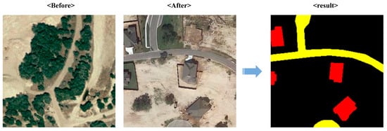
Figure 1. Remote sensing image change detection (RSICD).

The development of Natural Language Processing and Multimodal Technology provides an opportunity for the emergence of remote sensing image change captioning (RSICC). This task uses computer vision technology to extract bi-temporal image features and capture the spatiotemporal dependencies of objects therein. Then, it uses language-processing technology to describe the changes between bi-temporal images in human language. This intuitive text information can provide useful data value in auxiliary decision making. It can help relevant workers, researchers, and even non-professionals quickly understand surface changes. Moreover, with the help of deep learning technology, many text captions generated by RSICC tasks can also serve downstream tasks, such as Knowledge Graphs.

The current mainstream RSICC methods typically employ an end-to-end approach to construct model frameworks, with structural configurations generally comprising a backbone network, an encoder, and a language decoder. The encoder serves as a critical component of RSICC models, with functions primarily including capturing spatiotemporal differences, modeling contextual dependencies, and integrating bi-temporal features. Since the initial implementation of the RSICC task by Chouaf et al. [5] in 2021, its research scope has continuously expanded. The introduction of the first large-scale public dataset specifically for RSICC by Liu et al. [6] further accelerated the development of this task, leading to increasingly diverse methodologies. The core processing mechanisms of these models now cover mainstream architectures such as CNN, Transformer, and Mamba architectures. However, the classical RSICC approaches still face several interconnected challenges. These issues stem from the inherent characteristics of various core architectures. Most of the current RSICC methods construct encoders based on a single architecture, such as pure Transformer or pure Mamba, which means that the model performance may face trade-offs due to the specific characteristics and flaws of the core architecture. The exploration of hybrid architectures that leverage complementary advantages remains relatively scarce in the existing research. Moreover, the nature of the RSICC task itself and the choice of learning paradigms can also limit performance improvements. While the classical encoder–decoder approach is highly efficient, RSICC is essentially a process that transitions from visual feature processing to natural language generation. The emphasis on deep semantics has become a bottleneck for classical methods in enhancing the accuracy of descriptive sentences. Consequently, current and future research is increasingly trending toward multi-task collaborative enhancement.

Based on the above background, this paper proposes a Mamba–Transformer Hybrid Network (MTH-Net). The MTH-Net generally follows the shared-feature structure similar to classical encoder–decoder methods, effectively reducing the computational load of multi-task learning. At the encoder end, it incorporates the multi-class feature generation (MFG) module as a feature-processing hub, responsible for refining various types of features for different modeling tasks. Subsequently, the Spatiotemporal Difference Perception Network (SDPN) integrates both the Mamba and Transformer architectures to construct a symmetric Siamese network for analyzing spatiotemporal differences in bi-temporal images. The Mamba architecture focuses on modeling temporal context to learn progressive temporal changes, while the Transformer architecture specializes in spatial modeling to capture objects and dependencies across the entire image. Finally, spatiotemporal features are fused via a broadcasting mechanism and fed to the decoder. Furthermore, based on MTH-Net, we implemented two multi-task learning strategies, both of which achieved promising experimental results. Our main contributions include the following aspects:

• We constructed a multi-class feature generation (MFG) module. Working in synergy with the SDPN, it forms a systematic encoder workflow encompassing the complete feature-processing pipeline and employs a shared-feature-generation framework to enhance the multi-task learning efficiency.
• Within the SDPN, we built a symmetric Siamese network based on a Mamba–Transformer hybrid architecture. It leverages the strengths of both components for joint spatiotemporal change perception, further exploring the potential of applying structural symmetry in the RSICC field.
• Based on the MTH-Net framework, we experimentally validated two multi-task collaboration methods on public datasets: joint training with a unified loss function and explicit guidance for the CC task enhancement using generated CD masks. This provides valuable experience for subsequent diversified research in RSICC methods.

The subsequent contents of this article are structured as follows: Section 2 reviews previous work on remote sensing image change detection (RSICD), and remote sensing image change captioning (RSICC), as well as their interrelationships. Section 3 provides a detailed introduction to the MTH-Net model. Section 4 presents the experimental results and analysis. Section 5 concludes the paper and offers future perspectives.

2. Related Works

Remote sensing image change detection (RSICD) is closely related to the development of remote sensing image change captioning (RSICC), and, in this study, RSICD served as an auxiliary means to collaboratively enhance our main task: RSICC. This section briefly reviews the related work of these two tasks and their interrelationship.

2.1. Remote Sensing Image Change Detection (RSICD)

Remote sensing image change detection (RSICD) aims to detect change regions in bi-temporal RS images at the pixel level and present the localization of change regions through binary or semantic classification mask maps. Early RSICD methods mainly included algebra-based, transformation-based, and classification-based approaches [1]. Due to the superior feature representation capabilities of deep learning compared to traditional methods in change detection (CD), current methods primarily employ CNNs, Transformers, and Graph Convolutional Networks (GCNs) as feature extractors and classifiers. Li et al. [7] proposed a bi-temporal fusion strategy that promotes the interaction between bi-temporal features through a temporal feature interaction module, enabling the extraction of multi-level difference features. They also designed a guided refinement module to refine these multi-level features using cross-layer complementary information. Chen et al. [8] utilized a Transformer framework based on Siamese networks, where the Transformer refines the bi-temporal features extracted by a CNN using semantically marked image representations to enhance the model’s context and identify changes of interest in given bi-temporal images. Peng et al. [9] proposed the DDCNN model, constructing an end-to-end network that employs multiple upsampling attention units to capture internal associations across features at different levels, thereby discovering change features from spatial contextual information. In addition to the aforementioned supervised methods, unsupervised methods also demonstrate potential. Saha et al. [10] introduced the Deep Change Vector Analysis (DCVA) method, combining CVA with pretrained CNNs to extract changed pixels from spatial contextual information. Tang et al. [4] integrated GCNs with metric learning algorithms, using multi-scale dynamic GCN modules to capture rich contextual information from visual representations. Simultaneously, they extracted and analyzed spatial–spectral features from bi-temporal RS images and combined metric learning algorithms to generate reliable pseudo-labels for unsupervised training.

RSICD aims to identify pixel-level changes between bi-temporal images, while RSICC focuses on generating linguistic captions of change-related elements, such as objects, regions, trends, and relationships, at the semantic level.

2.2. Remote Sensing Image Change Captioning (RSICC)

As shown in Figure 2, the existing mainstream RSICC methods primarily adopt two strategies when constructing the overall model architecture: the classical encoder–decoder and multi-task collaborative enhancement.

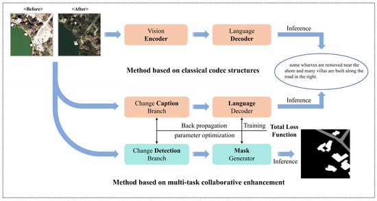
Figure 2. Schematic diagram of the RSICC method working based on the classical codec structure and multi-task cooperative enhancement.

For classical encoder–decoder methods, Chouaf et al. [5] first experimented with RSICC on aerial image sets. They used CNNs to extract bi-temporal image features, which were fused and then fed into a multimodal recurrent neural network (RNN) to generate descriptive sentences. Hoxha et al. [11] expanded on prior work by proposing an early-and-late bi-temporal visual feature fusion strategy and experimented with two decoders (RNN and Support Vector Machine (SVM)) for description generation. However, these CNN-based encoder methods, due to the sliding window operation of their convolutional kernels, often focus only on local regions of the image or sequence, presenting limitations for tasks like RSICC that require modeling contextual dependencies. The RSICCformer proposed by Liu et al. [6] introduced the Transformer architecture into both the encoder and decoder. It uses a pretrained ResNet101 [12] as the backbone network to extract basic features from bi-temporal RS images. The encoder, based on a cross-attention mechanism, takes bi-temporal features and difference features as Q and K (V) inputs, respectively, to enhance the change capture capability. A Transformer decoder then converts the features containing change representation information into descriptive sentences. They also constructed LEVIR-CC, the first large-scale public dataset for RSICC, providing a foundational model paradigm and data basis for the subsequent rapid development of RSICC research. PromptCC [13] first uses an image-level classifier to determine whether changes occurred in the bi-temporal images. The resulting prompts and visual embeddings are then fed together into a pretrained GPT-2, representing an initial attempt to leverage prompt learning techniques and the prior knowledge of pretrained large models for generating descriptions. PSNet [14] and ICT-Net [15] improved the model performance from the perspectives of multi-level and multi-scale feature extraction, respectively. The former gradually extracts multi-level features and then cross-enhances them via a cross-attention mechanism. The latter extracts multi-scale features through the backbone network and then employs a gated attention network for adaptive fusion, filtering out interference from irrelevant features. The SFT model proposed by Sun et al. [16] builds a Sparse Focal Attention network based on the traditional self-attention mechanism, achieving a stable performance at a lower computational cost. Compared to CNN-based methods, Transformer-based architectures significantly improve both the accuracy of generated captions and the overall model performance. However, the self-attention mechanism in Transformers inherently has quadratic computational complexity. Furthermore, when processing image sequence tasks, high-resolution inputs must be divided into longer sequence patches. Increasing the sequence length can lead to performance degradation, hindering the widespread application and scaling of RSICC methods, and global attention computation can introduce redundant information. RSCaMa [17] was the first to introduce the Mamba architecture for the RSICC task, effectively improving the computational efficiency and evaluation metrics through its bidirectional SSM mechanism for joint spatiotemporal modeling. Although the Mamba architecture enables more efficient long-range dependency modeling via its selective state space mechanism, its linear recurrent structure and parameter sharing across channels might limit its capacity for the dynamic interaction of fine-grained features across channels, potentially affecting its ability to capture changes involving small objects or high-frequency details.

Classical encoder–decoder methods have propelled the flourishing development of RSICC research. By presenting changes through descriptive sentences, change captioning (CC) achieves richer semantic-level expression compared to change detection (CD). It can not only use nouns such as “forest”, “road”, and “villages” to express change objects but can also use prepositions and other word types to describe the dependencies between change objects, such as “beside”, “along”, “appear”, and “disappear”, which improves human–computer interaction. However, due to their inherent operational characteristics, traditional CC tasks also face limitations: the quality of the generated descriptions often struggles to match the pixel-level precision of CD tasks, as illustrated in Figure 3. This also poses a challenge for the future development of the RSICC task. The emergence of multi-task collaborative enhancement methods for RSICC has become an effective approach to address this bottleneck in improving the caption quality. A representative example is the MCINet model proposed by Liu et al. [18], which integrates both RSICC and RSICD tasks within a single model architecture. Specifically, they constructed separate branches for the CC and CD tasks, employing similar encoder structures for deep features. Subsequently, dedicated decoders for each task at the decoder side output the descriptive sentences and change mask maps. During training, the optimizer uses a unified loss function, derived from the normalized sum of the two cross-entropy loss functions commonly used for the CC and CD tasks, to control gradient descent. This workflow offers two main advantages. First, the decoded captions and mask maps provide a more comprehensive change interpretation. Visually presenting both outputs can better meet user needs, allowing them to understand temporal RS image changes in the most suitable way. Second, joint training via the unified loss function establishes an effective synergistic and complementary mechanism between the two tasks. The unified loss combines the cross-entropy functions of both tasks: the CD branch provides pixel-level change localization, guiding the CC branch to focus on important semantic change regions, while the high-level semantic information generated by the CC branch can optimize the CD branch’s category discrimination capability, ultimately enhancing the performances of both branches. However, MCINet and similar multi-task collaborative methods, due to their dual-branch structure requiring separate processing paths for CC and CD, need to configure twice the number of core processing units in the encoder compared to classical encoder–decoder methods. This consequently introduces greater computational load. Furthermore, the dual-branch design is not conducive to achieving the sufficient dynamic interaction and joint optimization of parameters between the two tasks during learning.

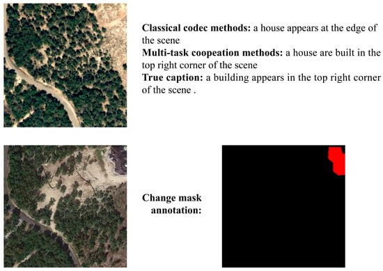
Figure 3. Examples of generating captions for the same scene based on the classical codec structure method and the multi-task collaborative enhancement method.

These methods have significantly contributed to the in-depth development and scale expansion of RSICC research. However, they still have limitations in terms of the overall structure of the model or core processing mechanisms. Our proposed MTH-Net employs a feature-sharing architecture and a core processing mechanism based on Mamba–Transformer to address the aforementioned issues. A detailed introduction to this model framework is provided in Section 3.

3. Methodology

As shown in Figure 4, the MTH-Net primarily consists of four components, including a backbone network based on Segformer-MiT-B1 [19], the multi-class feature generation (MFG) module, the Spatiotemporal Difference Perception Network (SDPN), and a dual-task decoder. Like previous RSICC methods, the MTH-Net still employs a universal encoder structure when constructing the overall framework, with only the decoding stage branching into separate paths. This approach facilitates the sharing of enhanced bi-temporal features between the decoders of the CC and CD tasks, enabling the model to be influenced by both learning tasks during iterative optimization and enhancing its ability to express change information. Given that previous methods [13,14,17] based on Vision Transformer [20] as the backbone network have demonstrated strong feature extraction capabilities, and considering that mainstream CD decoders typically employ UNet [21] architectures requiring multi-scale features as input to progressively refine spatial details and edge information, we select Segformer-MiT-B1 as the backbone network for extracting fundamental features (${\mathrm{F}}_{{\mathrm{t}}_{\mathrm{i}}}^{{\mathrm{T}}_{\mathrm{n}}}\in {\mathbb{R}}^{{\mathrm{C}}_{\mathrm{n}}\times {\mathrm{H}}_{\mathrm{n}}\times {\mathrm{W}}_{\mathrm{n}}}$) from bi-temporal images. Its hierarchical Transformer encoder architecture effectively balances ViT-level image processing performance with multi-scale feature output requirements. In the notation of this paper, F denotes the feature tensor, ${\mathrm{t}}_{\mathrm{i}}(\mathrm{i}=1,2)$ correspond to the before and after temporal states, respectively; ${\mathrm{T}}_{\mathrm{n}}(\mathrm{n}=1,2,3,4)$ represents the output of the n-th layer in the backbone; C, H, and W indicate the channel dimension, height, and width of the feature maps; and L denotes the token sequence length, which equals H × W. The deepest feature (${\mathrm{F}}_{{\mathrm{t}}_{\mathrm{i}}}^{{\mathrm{T}}_4}\in {\mathbb{R}}^{\mathrm{C}\times \mathrm{H}\times \mathrm{W}}$) is rich in semantic-level scene context information, which will be fed to the encoder composed of MFG and the SDPN. Through spatiotemporal modeling and difference feature perception, it captures spatial correlation information and temporal sequence context dependency information, ultimately generating a pair of shared bi-temporal features (${\mathrm{F}}_{{\mathrm{t}}_{\mathrm{i}}}^{\mathrm{s}\mathrm{h}\mathrm{a}\mathrm{r}\mathrm{e}}\in {\mathbb{R}}^{\mathrm{C}\times \mathrm{H}\times \mathrm{W}}$) enriched with critical change information. These features are then divided into two branches for the decoder. One branch is strengthened by residual units and sent to the language decoder, while the other is sent to the change mask generator. It is important to note that, since the performance study of RSICC remained our primary task in this study, and based on the experimental results of Liu et al. [17], we used a Transformer decoder [22] to generate descriptive sentences for the CC task to ensure the model performance. We employed the CD decoder from MCINet [18] for the change mask generation.

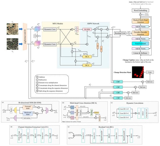
Figure 4. The overall structure of the MTH-Net is shown in the figure. It consists of the backbone network (image feature extractor), multi-class feature generation (MFG) module, Spatiotemporal Difference Perception Network (SDPN), and dual-task decoder. Panels (a,b,d) are adapted from [23].

3.1. Multi-Class Feature Generation (MFG) Module

In Figure 4, the yellow area represents the MFG component. After the backbone network extracts basic features from bi-temporal images, the deepest feature (${\mathrm{F}}_{{\mathrm{t}}_{\mathrm{i}}}^{{\mathrm{T}}_4} (\mathrm{i}=1, 2)$) is appended with position embeddings to obtain ${\mathrm{F}}_{{\mathrm{t}}_{\mathrm{i}}}^{(0)}\in {\mathbb{R}}^{\mathrm{L}\times \mathrm{C}}$, primarily to assist the model in distinguishing semantic features at different spatial locations. To address the irregular multi-scale object distribution characteristics of RS images, we constructed the multi-class feature generation (MFG) module as the hub for machining bi-temporal features. This module incorporates dynamic convolutions ([18], p. 5), employing three differently sized convolution kernels to concurrently extract multi-scale information from the horizontal, vertical, and local perspectives from ${\mathrm{F}}_{{\mathrm{t}}_{\mathrm{i}}}^{(0)}$. Subsequently, a 1 × 1 convolution is used to fuse this information and implement dynamic weight control, enabling the model to learn richer semantic representations, as illustrated in Figure 4c. Based on the multi-scale fused feature (${\mathrm{F}}_{{\mathrm{S}}_{\mathrm{i}}}^{(l)}\in {\mathbb{R}}^{\mathrm{L}\times \mathrm{C}}$), we perform two operations: differencing and sequence dimension concatenating, resulting in the spatial difference feature (${\mathrm{F}}_{\mathrm{dif}}^{(l)}\in {\mathbb{R}}^{\mathrm{L}\times \mathrm{C}}$) and temporal connection feature (${\mathrm{F}}_{\mathrm{t}\mathrm{i}\mathrm{m}\mathrm{e}}^{(l)}\in {\mathbb{R}}^{2\mathrm{L}\times \mathrm{C}}$). The ${\mathrm{F}}_{{\mathrm{S}}_{\mathrm{i}}}^{(l)}, {\mathrm{F}}_{\mathrm{dif}}^{(l)}, \mathrm{and} {\mathrm{F}}_{\mathrm{t}\mathrm{i}\mathrm{m}\mathrm{e}}^{(l)}$ are collectively fed as the output of MFG to the SDPN for parallel spatiotemporal modeling. The multi-class features outputted after MFG processing enhance the SDPN’s ability to perceive local and multi-scale changes. The specific process can be represented as follows:

$${\mathrm{F}}_{{\mathrm{t}}_{\mathrm{i}}}^{(0)}={\Phi }_{\mathrm{P}\mathrm{o}\mathrm{s}}({\mathrm{F}}_{{\mathrm{t}}_{\mathrm{i}}}^{{\mathrm{T}}_4}),$$

(1)

$${\mathrm{F}}_{{\mathrm{S}}_{\mathrm{i}}}^{(l)}={\Phi }_{\mathrm{D}\mathrm{y}\mathrm{c}\mathrm{o}\mathrm{n}\mathrm{v}}({\mathrm{F}}_{{\mathrm{t}}_{\mathrm{i}}}^{(0)}),$$

(2)

$${\mathrm{F}}_{\mathrm{d}\mathrm{i}\mathrm{f}}^{(l)}={\mathrm{F}}_{{\mathrm{S}}_2}^{(l)}-{\mathrm{F}}_{{\mathrm{S}}_1}^{(l)},$$

(3)

$${\mathrm{F}}_{\mathrm{t}\mathrm{i}\mathrm{m}\mathrm{e}}^{(l)}=\mathrm{C}\mathrm{o}\mathrm{n}\mathrm{c}\mathrm{a}{\mathrm{t}}_{\mathrm{L}}({\mathrm{F}}_{{\mathrm{S}}_1}^{(l)}, {\mathrm{F}}_{{\mathrm{S}}_2}^{(l)}),$$

(4)

Here, ${\Phi }_{\mathrm{P}\mathrm{o}\mathrm{s}}( )$ represents the position embedding. ${\Phi }_{\mathrm{D}\mathrm{y}\mathrm{c}\mathrm{o}\mathrm{n}\mathrm{v}}( )$ represents the dynamic convolution operation. $\mathrm{C}\mathrm{o}\mathrm{n}\mathrm{c}\mathrm{a}{\mathrm{t}}_{\mathrm{L}}( )$ and $\mathrm{C}\mathrm{o}\mathrm{n}\mathrm{c}\mathrm{a}{\mathrm{t}}_{\mathrm{C}}( )$ represent concatenating along the sequence and channel dimensions, respectively. i represents temporal, and (l = 1, 2,…, N) represents the number of encoder iteration layers.

3.2. Spatiotemporal Difference Perception Network (SDPN)

The SDPN is represented by the blue region in Figure 4. Within the SDPN, we have constructed a novel architecture for spatiotemporal modeling. Inspired by the M-T DHB structure of the MTAIR network [24], which achieved exceptional results in image restoration tasks, we designed our Mamba–Transformer-integrated architecture as the core processing mechanism of the encoder. The M-T DHB mode is illustrated in Figure 5, while Figure 6 depicts our SDPN. Since tasks like CC and CD involve processing bi-temporal images, a dual-branch encoder structure is commonly employed. If configured like M-T DHB, each temporal branch requires a pair of processing units based on Mamba and Transformer. This implies that four core processing units are required for context modeling in the encoder. Furthermore, if multiple modeling tasks are involved, the number of configurations increases accordingly, which could be computationally burdensome for RSICC models. Therefore, we improved upon the M-T DHB structure to better accommodate the characteristics of RSICC tasks. Unlike M-T DHB, our method does not adopt cross-broadcasting or stacking fusion to integrate the two architectures. We allocate different modeling tasks based on the strengths and weaknesses of the two mainstream architectures. This approach reduces redundant information and further leverages the Bi-SSM’s advantage in long-range context modeling, preventing the overfitting that could occur with the two architectures, leading to an unstable model performance. The SDPN requires only three Bi-SSM/MCA units per iteration to meet the needs of temporal and spatial modeling.

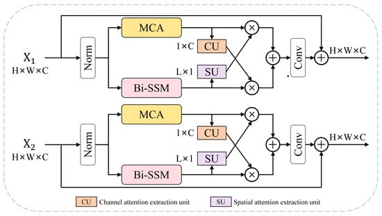
Figure 5. The renderings of the RSICC encoder constructed in the manner of M-T DN [24] are shown above. CU and SU denote the extraction channel and spatial attention operation, respectively.

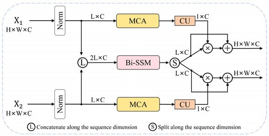
Figure 6. Our SDPN constructs the Mamba–Transformer integration architecture as above, wherein difference perception and other calculations are omitted, solely to demonstrate the distinction between our method and the M-T DN module.

Each SDPN iteration layer primarily consists of an SSM (state space model) unit and two MCA (multi-head cross-attention) units. The core innovation of Mamba, a powerful variant of the SSM, lies in its selective scan mechanism. Since SSM parameters such as Δ, B, and C are input-dependent, when processing continuous time series with “Before” and “After” attributes, Mamba becomes “activated” and significantly updates its state upon encountering tokens from potentially changing regions in the input sequence, integrating these critical pieces of information into the contextual memory. This data-driven filtering capability enables it to efficiently and accurately capture the “signals” within the temporal sequence, which determines its high compatibility with RSICC and similar temporal analysis-based image-processing tasks. As shown in Figure 4a, we utilize the Mamba architecture based on bidirectional SSM from the RSCaMa encoder, whose design philosophy evolved from Vision Mamba (ViM) [25]. The original Mamba [26] employs a unidirectional selective scan mechanism in its SSM, making it better suited for NLP tasks. However, when processing image sequences with spatial structures, this approach may lead to contextual information loss. ViM enhances the original architecture by implementing bidirectional scanning and fusing the hidden states from both directions, thereby addressing this limitation. The SSM unit employed in our SDPN preserves causal convolutions within both scanning directions while implementing the bidirectional selective scan mechanism. This design ensures that the extracted intrinsic temporal dependencies between tokens follow the “before-to-after” sequential logic chain when performing temporal modeling along the full-time sequence. In contrast, standard 2D convolution disregards this temporal order and mixes information from different time points, potentially leading to incorrect temporal evolution patterns being learned, which is not conducive to the ultimate objectives of language generation tasks. For ease of expression, this architecture will be referred to as the Bi-SSM (Bidirectional SSM) in subsequent discussions. To preserve the temporal order of the sequence, we employ the Bi-SSM for temporal modeling on the temporal connection features (${\mathrm{F}}_{\mathrm{t}\mathrm{i}\mathrm{m}\mathrm{e}}^{(l)}\in {\mathbb{R}}^{2\mathrm{L}\times \mathrm{C}}$) from the MFG output. The Bi-SSM, with its linear complexity and efficient hardware algorithms, offers a higher computational cost-effectiveness when processing sequences of 2L length compared to MCA. MCA, in contrast, is utilized for spatial modeling on multi-scale fusion features (${\mathrm{F}}_{{\mathrm{S}}_{\mathrm{i}}}^{(l)}\in {\mathbb{R}}^{\mathrm{L}\times \mathrm{C}} (\mathrm{i}=1, 2)$). Leveraging the fine-grained feature extraction capability of the multi-head attention mechanism, MCA can effectively identify the spatial distribution of complex scenes in the sequence and capture local and global dependencies between objects within the scenes.

To better integrate the advantages of the Mamba and Transformer architectures, the SDPN employs the Bi-SSM and MCA to perform temporal and spatial modeling in parallel, followed by fusion through a broadcasting mechanism. The MFG outputs multi-scale fused features (${\mathrm{F}}_{{\mathrm{S}}_{\mathrm{i}}}^{(l)}\in {\mathbb{R}}^{\mathrm{L}\times \mathrm{C}}$), temporal connection features (${\mathrm{F}}_{\mathrm{t}\mathrm{i}\mathrm{m}\mathrm{e}}^{(l)}\in {\mathbb{R}}^{2\mathrm{L}\times \mathrm{C}}$), and spatial difference features (${\mathrm{F}}_{\mathrm{dif}}^{(l)}\in {\mathbb{R}}^{\mathrm{L}\times \mathrm{C}}$) to the SDPN. The difference features (${\mathrm{F}}_{\mathrm{dif}}^{(l)}$) are simultaneously applied to both architectures, significantly enhancing the model’s ability to perceive spatiotemporal changes. As shown in the blue region of Figure 4, ${\mathrm{F}}_{{\mathrm{dif}}_{\mathrm{m}}}\in {\mathbb{R}}^{2\mathrm{L}\times \mathrm{C}}$ is input into the activation branch of the Bi-SSM, multiplied with the output of the SSM unit, utilizing the difference features to guide the Bi-SSM to selectively focus on features closely related to changes in the context of the time sequence. The MCA processing method is similar to previous RSICC methods based on Transformers, where ${\mathrm{F}}_{{\mathrm{S}}_{\mathrm{i}}}^{(l)}\in {\mathbb{R}}^{\mathrm{L}\times \mathrm{C}}$ and ${\mathrm{F}}_{{\mathrm{dif}}_{\mathrm{t}}}\in {\mathbb{R}}^{\mathrm{L}\times \mathrm{C}}$ are used as Q and K (V) in the MCA, respectively; its structure is shown in Figure 4b. MCA captures spatial objects in images at times ${\mathrm{t}}_1, {\mathrm{t}}_2$ and their potential relationships through multiple heads. The difference features, serving as K (V), enhance the weights of change-related features in the bi-temporal image (Q), outputting features (${\mathrm{F}}_{{\mathrm{T}}_{\mathrm{i}}}^{(l)}\in {\mathbb{R}}^{\mathrm{L}\times \mathrm{C}}$) containing spatial change information.

For the output features of the Bi-SSM and MCA processing units, we treat the output of the Bi-SSM unit as the main propagation direction and employ a channel attention extraction unit to process the output (${\mathrm{F}}_{{\mathrm{T}}_{\mathrm{i}}}^{(l)}$) of the MCA. As shown in Figure 4d, the channel attention extraction unit (CU) consists of global average pooling and the fully connected layers, capable of transforming spatial features (${\mathrm{F}}_{{\mathrm{T}}_{\mathrm{i}}}^{(l)}$) into channel weights (${\mathrm{S}}_{{\mathrm{T}}_{\mathrm{i}}}^{(l)}\in {\mathbb{R}}^{1\times \mathrm{C}}$). Through residual connections and broadcasting operations, the channel weights are efficiently fused with the output features (${\mathrm{F}}_{{\mathrm{M}}_{\mathrm{i}}}^{(l)}\in {\mathbb{R}}^{\mathrm{L}\times \mathrm{C}}$) of the Bi-SSM unit. The attention weights, which contain fine-grained channel information, are propagated along the spatial dimension to the temporal features (${\mathrm{F}}_{{\mathrm{M}}_{\mathrm{i}}}^{(l)}$) and output the shared features (${\mathrm{F}}_{{\mathrm{t}}_{\mathrm{i}}}^{\mathrm{s}\mathrm{h}\mathrm{a}\mathrm{r}\mathrm{e}}\in {\mathbb{R}}^{\mathrm{C}\times \mathrm{H}\times \mathrm{W}}$) for the CC and CD decoders, thereby achieving the complementary advantages of the two architectures. Compared to the explicit expansion approach of directly multiplying the outputs of the Bi-SSM and MCA, the SDPN utilizes the CU to broadcast only the channel weights from the spatial path’s output to the backbone features of the temporal path. This design simultaneously achieves both information complementarity and gating optimization. The refined weights derived from the MCA branch can selectively enhance or suppress individual channels in the temporal features output by the Bi-SSM, ensuring that only the most salient spatiotemporal change information propagates forward, thereby significantly improving the model’s robustness against background interference. The specific computation process of the SDPN can be expressed as follows:

$${\mathrm{F}}_{{\mathrm{t}}_{\mathrm{i}}}^{\mathrm{s}\mathrm{h}\mathrm{a}\mathrm{r}\mathrm{e}}={\mathrm{F}}_{{\mathrm{M}}_{\mathrm{i}}}^{(l)}\times {\mathrm{S}}_{{\mathrm{T}}_{\mathrm{i}}}^{(l)}+{\mathrm{F}}_{{\mathrm{M}}_{\mathrm{i}}}^{(l)},$$

(5)

$${\mathrm{F}}_{{\mathrm{M}}_1}^{(l)},{\mathrm{F}}_{{\mathrm{M}}_2}^{(l)}={\Phi }_{\mathrm{Split}}({\mathrm{F}}_{\mathrm{M}}^{(l)}),$$

(6)

$${\mathrm{F}}_{\mathrm{M}}^{(l)}={\Phi }_{\mathrm{B}\mathrm{i}-\mathrm{S}\mathrm{S}\mathrm{M}}({\mathrm{F}}_{\mathrm{t}\mathrm{i}\mathrm{m}\mathrm{e}}^{(l)}, {\mathrm{F}}_{{\mathrm{dif}}_{\mathrm{m}}}),$$

(7)

$${\mathrm{S}}_{{\mathrm{T}}_{\mathrm{i}}}^{(l)}={\Phi }_{\mathrm{C}\mathrm{U}}({\mathrm{F}}_{{\mathrm{T}}_{\mathrm{i}}}^{(l)}),$$

(8)

$${\mathrm{F}}_{{\mathrm{T}}_{\mathrm{i}}}^{(l)}={\Phi }_{\mathrm{M}\mathrm{C}\mathrm{A}}({\mathrm{F}}_{{\mathrm{S}}_{\mathrm{i}}}^{(l)}, {\mathrm{F}}_{{\mathrm{dif}}_{\mathrm{t}}}, {\mathrm{F}}_{{\mathrm{dif}}_{\mathrm{t}}}),$$

(9)

$${\mathrm{F}}_{{\mathrm{dif}}_{\mathrm{m}}}=\mathrm{C}\mathrm{o}\mathrm{n}\mathrm{c}\mathrm{a}{\mathrm{t}}_{\mathrm{L}}({\mathrm{F}}_{\mathrm{dif}}^{(l)}, {\mathrm{F}}_{\mathrm{dif}}^{(l)}),$$

(10)

$${\mathrm{F}}_{{\mathrm{dif}}_{\mathrm{t}}}={\mathrm{F}}_{{\mathrm{S}}_{\mathrm{i}}}^{(l)}\times {\mathrm{F}}_{\mathrm{dif}}^{(l)},$$

(11)

Here, ${\Phi }_{\mathrm{S}\mathrm{p}l\mathrm{i}\mathrm{t}}( )$ denotes the splitting tensor along the sequence dimension. ${\Phi }_{\mathrm{C}\mathrm{U}}( )$ is the channel attention extraction unit.

3.3. Decoder

We practice two RSICC methods using multi-task collaboration based on the MTH-Net, with the joint training based on the total loss function and the CC enhancement explicitly guided by the generated CD masks. The former requires using two kinds of decoders: the CC task’s language decoder and the CD task’s change mask generator.

3.3.1. Transformer Decoder

In this study, we utilized the Transformer decoder to generate descriptive sentences. As shown in Figure 4, the standard Transformer decoder layer consists of three sublayers: a masked self-attention layer, an encoder–decoder attention layer based on cross-attention, and a feed-forward network layer. A residual connection and layer normalization accompany each sublayer. Finally, a linear layer and a softmax layer are applied to generate the probability distribution of all words in the vocabulary at each time step position, and the word with the highest probability is selected to generate the sentence. During the training phase, the Transformer language decoder operates in Teacher Forcing mode, while in the inference and prediction phase, it runs autoregressively. The processes are briefly elaborated in the following sections.

The bi-temporal shared features (${\mathrm{F}}_{{\mathrm{t}}_{\mathrm{i}}}^{\mathrm{s}\mathrm{h}\mathrm{a}\mathrm{r}\mathrm{e}}$) output by the SDPN are fed into the residual unit shown in Figure 4e to perform the deep integration of the bi-temporal features, further highlighting the key change information. The processed visual embeddings and text token sequences are then input into the Transformer decoder from two directions to generate descriptive sentences in an autoregressive manner.

The output side of the Transformer decoder is configured with a set of linear and softmax layers. The linear layer maps the embedding representation (${\mathrm{S}}_{\mathrm{c}\mathrm{a}\mathrm{p}}\in {\mathbb{R}}^{\mathrm{N}\times \mathrm{e}\mathrm{m}\mathrm{d}}$) (N and emd represent the sentence length and embedding dimension, respectively), containing multimodal correlation information, to $\mathrm{Y}\in {\mathbb{R}}^{\mathrm{N}\times \mathrm{V}}$ (V represents the vocabulary size), which includes the word prediction vector (${\mathrm{y}}_{\mathrm{t}}=[{\mathrm{y}}_{\mathrm{t}}^{(1)}, {\mathrm{y}}_{\mathrm{t}}^{(2)},\dots ,{\mathrm{y}}_{\mathrm{t}}^{(\mathrm{V})}]$) at time step t, that is, the predicted score of the vocabulary’s word in the corresponding sentence position when at time step t. The softmax function then converts ${\mathrm{y}}_{\mathrm{t}}$ into the probability distribution vector (${\mathrm{p}}_{\mathrm{t}}$) of the corresponding word, which generates the word at the current time step position in the sentence. The process can be represented as follows:

$${\mathrm{p}}_{\mathrm{t}}=\mathrm{S}\mathrm{o}\mathrm{f}\mathrm{t}\max ({\mathrm{y}}_{\mathrm{t}})={\displaystyle \frac{\exp ({\mathrm{y}}_{\mathrm{t}})}{{\displaystyle \sum _{\mathrm{i}=1}^{\mathrm{V}}\exp ({\mathrm{y}}_{\mathrm{t}}^{\mathrm{i}})}}},$$

(12)

$${\mathrm{p}}_{\mathrm{t}}=[{\mathrm{p}}_{\mathrm{t}}^{(1)}, {\mathrm{p}}_{\mathrm{t}}^{(2)},\dots ,{\mathrm{p}}_{\mathrm{t}}^{(\mathrm{V})}] ,$$

(13)

3.3.2. Change Mask Generator

When introducing the RSICD task for joint training, we adopted the UNet-like decoder structure used in the MCINet [18]. The shared features (${\mathrm{F}}_{{\mathrm{t}}_{\mathrm{i}}}^{\mathrm{s}\mathrm{h}\mathrm{a}\mathrm{r}\mathrm{e}}$) output by the encoder and the multi-scale features (${\mathrm{F}}_{{\mathrm{t}}_{\mathrm{i}}}^{{\mathrm{T}}_{\mathrm{n}}}\in {\mathbb{R}}^{{\mathrm{C}}_{\mathrm{n}}\times {\mathrm{H}}_{\mathrm{n}}\times {\mathrm{W}}_{\mathrm{n}}} (\mathrm{n}=1, 2, 3)$) output by the backbone are input into the corresponding CBF layers. These layers associate and fuse the change information in the bi-temporal features by calculating the difference features and cosine similarity and output the fusion features (${\mathrm{F}}_{\mathrm{f}\mathrm{u}\mathrm{s}}^{{\mathrm{T}}_l}\in {\mathbb{R}}^{{\mathrm{C}}_l\times {\mathrm{H}}_l\times {\mathrm{W}}_l}$) of the corresponding layers. Then, the CD decoder integrates this information layer by layer from deep to shallow through the upsampling operation based on deconvolution and the residual connection. Finally, using a 1 × 1 convolutional layer and a softmax layer, we predict the classification score (${\mathrm{F}}_{\mathrm{c}\mathrm{l}\mathrm{s}}^{{\mathrm{T}}_1}\in {\mathbb{R}}^{\mathrm{num}\times {\mathrm{H}}_1\times {\mathrm{W}}_1}$) and probability distribution (${\mathrm{p}}_{\mathrm{C}\mathrm{D}}\in {\mathbb{R}}^{\mathrm{num}\times {\mathrm{H}}_1\times {\mathrm{W}}_1}$) for each pixel position in the change mask, where num represents the number of classifications. The specific process is as follows:

$$\begin{array}{l}{\mathrm{p}}_{\mathrm{C}\mathrm{D}}=\mathrm{s}\mathrm{o}\mathrm{f}\mathrm{t}\max (\mathrm{C}\mathrm{o}\mathrm{n}{\mathrm{v}}_{1\times 1}({\mathrm{F}}_{\mathrm{c}\mathrm{l}\mathrm{s}}^{{\mathrm{T}}_1})),\\ \mathrm{F}\mathrm{o}\mathrm{r} l=4,\dots ,1:\\ {\mathrm{F}}_{\mathrm{c}\mathrm{l}\mathrm{s}}^{{\mathrm{T}}_l}=\mathrm{D}\mathrm{e}\mathrm{C}\mathrm{o}\mathrm{n}\mathrm{v}({\mathrm{F}}_{\mathrm{f}\mathrm{u}\mathrm{s}}^{{\mathrm{T}}_l}+{\mathrm{F}}_{\mathrm{c}\mathrm{l}\mathrm{s}}^{{\mathrm{T}}_{l+1}}),\\ {\mathrm{F}}_{\mathrm{f}\mathrm{u}\mathrm{s}}^{{\mathrm{T}}_l}={\Phi }_{\mathrm{C}\mathrm{B}\mathrm{F}}({\mathrm{F}}_{{\mathrm{t}}_{\mathrm{i}}}^{{\mathrm{T}}_l}),\end{array}$$

(14)

When l = 4, the input of ${\Phi }_{\mathrm{C}\mathrm{B}\mathrm{F}}( )$ is ${\mathrm{F}}_{{\mathrm{t}}_{\mathrm{i}}}^{\mathrm{s}\mathrm{h}\mathrm{a}\mathrm{r}\mathrm{e}}$, $\mathrm{D}\mathrm{e}\mathrm{c}\mathrm{o}\mathrm{n}\mathrm{v}( )$ denotes deconvolution, and operations such as $\mathrm{B}\mathrm{N}( )$ and $\mathrm{C}\mathrm{o}\mathrm{n}\mathrm{v}( )$ in the structural cohesion part are omitted in the formula. The ${\Phi }_{\mathrm{C}\mathrm{B}\mathrm{F}}( )$ operation is formulated as follows:

$${\Phi }_{\mathrm{C}\mathrm{B}\mathrm{F}}({\mathrm{F}}_{{\mathrm{t}}_{\mathrm{i}}}^{{\mathrm{T}}_l})=\mathrm{C}\mathrm{o}\mathrm{n}{\mathrm{v}}_{1\times 1}(\mathrm{Re}\mathrm{L}\mathrm{U}(\mathrm{B}\mathrm{N}(\mathrm{C}\mathrm{o}\mathrm{n}{\mathrm{v}}_{3\times 3}(\mathrm{F})))),$$

(15)

$$\mathrm{F}=\mathrm{C}\mathrm{o}\mathrm{n}\mathrm{c}\mathrm{a}{\mathrm{t}}_{\mathrm{C}}({\mathrm{F}}_{{\mathrm{t}}_1}^{{\mathrm{T}}_l}, \mathrm{S}, {\mathrm{F}}_{{\mathrm{t}}_2}^{{\mathrm{T}}_l}),$$

(16)

$$\mathrm{S}=\mathrm{C}\mathrm{o}\mathrm{n}{\mathrm{v}}_{3\times 3}({\mathrm{F}}_{{\mathrm{t}}_2}^{{\mathrm{T}}_l}-{\mathrm{F}}_{{\mathrm{t}}_1}^{{\mathrm{T}}_l})+\mathrm{Cos}({\mathrm{F}}_{{\mathrm{t}}_1}^{{\mathrm{T}}_l}, {\mathrm{F}}_{{\mathrm{t}}_2}^{{\mathrm{T}}_l}),$$

(17)

3.4. The Method of Explicitly Guided RSICC Enhancement by the Generated RSICD Mask

In the current RSICC enhancement method based on multi-task collaboration, in addition to joint training using the total loss function obtained after normalizing the CC and CD loss functions, it also includes a method adopted by Liu et al. [27] in MV-CC to enhance the performance of the RSICC model by using the generated CD mask. Unlike the joint training method, this explicit guidance method appropriately decouples the CC and CD tasks in the training optimization phase. As shown in Figure 7, specifically, this method performs a broadcasting operation on the enhanced visual features output by the RSICC encoder using the already-generated change segmentation mask, guiding the language decoder to generate more accurate captions by utilizing pixel-level change discriminative information from the CD feature map. Only the cross-entropy loss function of the CC task is used during training optimization.

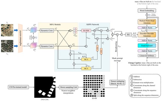
Figure 7. The workflow of introducing the generated CD mask data to explicitly guide the RSICC enhancement method is shown in the figure above. The model’s main composition is still based on the MTH-Net.

In practice, we first needed to collect CD masks from the same image set as the CC task. To ensure the objectivity of the experiment, we still used the MTH-Net to implement this method in this study. We utilized the pretrained models saved during the joint training stage to generate new supervised CD mask sets via inference. In order to prevent the embedding representations of the two tasks from generating shape conflicts in the broadcast phase, we also needed to downsample these CD masks during the data-loading process to match the visual embeddings of the CC encoder. The processing process of each batch of CD masks ($\mathrm{M}\mathrm{a}{\mathrm{sk}}_{\mathrm{C}\mathrm{D}}\in {\mathbb{R}}^{{\mathrm{H}}_{\mathrm{C}\mathrm{D}}\times {\mathrm{W}}_{\mathrm{C}\mathrm{D}}}$) is as follows:

$${\mathrm{Z}}_{\mathrm{C}\mathrm{D}}=\mathrm{I}\mathrm{n}\mathrm{t}\mathrm{e}\mathrm{r}\mathrm{p}\mathrm{o}\mathrm{l}\mathrm{a}\mathrm{t}\mathrm{e}(\mathrm{M}\mathrm{a}\mathrm{s}{\mathrm{k}}_{\mathrm{C}\mathrm{D}}, ‘\mathrm{n}\mathrm{e}\mathrm{a}\mathrm{r}\mathrm{e}\mathrm{s}\mathrm{t}’)\in {\mathbb{R}}^{{\mathrm{H}}_{\mathrm{C}\mathrm{C}}\times {\mathrm{W}}_{\mathrm{C}\mathrm{C}}\times 1},$$

(18)

Here, ${\mathrm{H}}_{\mathrm{C}\mathrm{C}}$ and ${\mathrm{W}}_{\mathrm{C}\mathrm{C}}$ represent the size of the shared feature (${\mathrm{F}}_{{\mathrm{t}}_{\mathrm{i}}}^{\mathrm{s}\mathrm{h}\mathrm{a}\mathrm{r}\mathrm{e}}$). $\mathrm{I}\mathrm{n}\mathrm{t}\mathrm{e}\mathrm{r}\mathrm{p}\mathrm{o}\mathrm{l}\mathrm{a}\mathrm{t}\mathrm{e}( )$ denotes downsampling via the interpolation operation, which is nearest-neighbor interpolation, to match the $\mathrm{M}\mathrm{a}{\mathrm{sk}}_{\mathrm{C}\mathrm{D}}$ feature map size of 256 × 256 to the size of the shared feature, generating the guidance weight (${\mathrm{Z}}_{\mathrm{C}\mathrm{D}}\in {\mathbb{R}}^{{\mathrm{H}}_{\mathrm{C}\mathrm{C}}\times {\mathrm{W}}_{\mathrm{C}\mathrm{C}}\times 1}$). The bi-temporal shared feature (${\mathrm{F}}_{{\mathrm{t}}_{\mathrm{i}}}^{\mathrm{s}\mathrm{h}\mathrm{a}\mathrm{r}\mathrm{e}}$) is concatenated along the channel dimension to obtain the fused feature (${\mathrm{F}}_{\mathrm{C}\mathrm{C}}^{\mathrm{f}\mathrm{u}\mathrm{s}}\in {\mathbb{R}}^{{\mathrm{H}}_{\mathrm{C}\mathrm{C}}\times {\mathrm{W}}_{\mathrm{C}\mathrm{C}}\times 2\mathrm{C}}$). The guidance weight (${\mathrm{Z}}_{\mathrm{C}\mathrm{D}}$) is broadcast to the ${\mathrm{F}}_{\mathrm{C}\mathrm{C}}^{\mathrm{f}\mathrm{u}\mathrm{s}}$ via the Hadamard product, followed by the deep fusion of pixel-level and semantic-level change information using the residual unit mentioned in Figure 4e, and is finally fed into the Transformer decoder to generate descriptive sentences. The process is represented as follows:

$${\mathrm{F}}_{\mathrm{C}\mathrm{C}}^{\mathrm{f}\mathrm{u}\mathrm{s}}=\mathrm{C}\mathrm{o}\mathrm{n}\mathrm{c}\mathrm{a}{\mathrm{t}}_{\mathrm{C}}({\mathrm{F}}_{{\mathrm{t}}_1}^{\mathrm{s}\mathrm{h}\mathrm{a}\mathrm{r}\mathrm{e}}, {\mathrm{F}}_{{\mathrm{t}}_2}^{\mathrm{s}\mathrm{h}\mathrm{a}\mathrm{r}\mathrm{e}})\in {\mathbb{R}}^{{\mathrm{H}}_{\mathrm{C}\mathrm{C}}\times {\mathrm{W}}_{\mathrm{C}\mathrm{C}}\times 2\mathrm{C}}$$

(19)

$${\mathrm{F}}_{\mathrm{f}\mathrm{u}\mathrm{s}}={\Phi }_{\mathrm{R}\mathrm{e}\mathrm{s}}(\mathrm{a}{\mathrm{F}}_{\mathrm{C}\mathrm{C}}^{\mathrm{f}\mathrm{u}\mathrm{s}}\odot {\mathrm{Z}}_{\mathrm{C}\mathrm{D}}+(1-\mathrm{a}){\mathrm{F}}_{\mathrm{C}\mathrm{C}}^{\mathrm{f}\mathrm{u}\mathrm{s}})\in {\mathbb{R}}^{\mathrm{L}\times \mathrm{C}}$$

(20)

$${\mathrm{S}}_{\mathrm{c}\mathrm{a}\mathrm{p}}={\Phi }_{\mathrm{D}\mathrm{e}\mathrm{c}\mathrm{o}\mathrm{d}\mathrm{e}\mathrm{r}}({\mathrm{F}}_{\mathrm{f}\mathrm{u}\mathrm{s}})\in {\mathbb{R}}^{\mathrm{N}\times \mathrm{e}\mathrm{m}\mathrm{d}}$$

(21)

In the above equation, the parameter (a) represents the learnable weight that adaptively controls the fusion ratio between the mask-guided features and the original features.

This method of using generated CD mask data to explicitly guide RSICC enhancement reduces the number of parameters by decoupling the two tasks to prune the RSICC framework based on multi-task collaboration. In addition, this method is flexible in data acquisition, as higher-quality change masks can be obtained in real practice through various SOTA methods specifically targeting RSICD, thereby providing more precise guidance for RSICC.

3.5. The Objective Function for Training

It should be noted that although our primary goal is still to promote the improvement in the CC task performance, in actual training, we expect CC and CD to generate high-quality captions and change masks. This is to avoid situations in joint training where a poor performance in one task might lead to the transmission of erroneous change information and misleading signals during the optimization of shared parameters. Therefore, the joint training method needs to use two cross-entropy loss functions commonly applied in the CC and CD tasks and then convert them into a total loss function as the training objective to maintain the training stability of the two tasks, while the method that generates CD masks to guide CC enhancement only needs the cross-entropy loss of CC for training, as it decouples the CC and CD tasks.

The CC task optimizes the model parameters by minimizing the difference between the probability distribution of the predicted word and the true distribution of the reference label word. The loss function can be expressed as follows:

$$\mathrm{L}\mathrm{o}\mathrm{s}{\mathrm{s}}_{\mathrm{c}\mathrm{a}\mathrm{p}}=-{\displaystyle \frac{1}{\mathrm{L}}}{\displaystyle \sum _{l=1}^{\mathrm{L}}{\displaystyle \sum _{v=1}^{\mathrm{V}}{\mathrm{y}}_l^{(v)}}\log ({\mathrm{p}}_l^{(v)})}$$

(22)

Here, L is the sentence length, V is the vocabulary size, ${\mathrm{y}}_l^{(v)}$ represents whether the lth word in the sentence corresponds to the vocabulary index (v), and ${\mathrm{p}}_l^{(v)}$ represents the probability of predicting that the lth word in the sentence is v.

The CD task optimizes the model parameters by minimizing the cross-entropy loss between the classification probability distribution and the true distribution at each pixel position of the predicted change mask map. The loss function can be expressed as follows:

$$\mathrm{L}\mathrm{o}\mathrm{s}{\mathrm{s}}_{\det }=-{\displaystyle \frac{1}{\mathrm{H}\times \mathrm{W}}}{\displaystyle \sum _{\mathrm{h}=1,\mathrm{w}=1}^{\mathrm{H},\mathrm{W}}{\displaystyle \sum _{j=1}^{\mathrm{C}}{\tilde{\mathrm{y}}}_{\mathrm{h}\mathrm{w}}^{(\mathrm{j})}}\log ({\mathrm{p}}_{\mathrm{h}\mathrm{w}}^{(\mathrm{j})})}$$

(23)

Here, C is the number of change mask classifications, H and W are the visual feature sizes, ${\tilde{\mathrm{y}}}_{\mathrm{h}\mathrm{w}}^{(\mathrm{j})}$ represents whether the true annotation is classified as j at pixel (h,w), and ${\mathrm{p}}_{\mathrm{h}\mathrm{w}}^{(\mathrm{j})}$ represents the probability that the predicted classification at pixel (h,w) is classified as j.

A normalized scaling method is adopted in [18] to calculate the total loss function for joint training, which can be formulated as follows:

$$\mathrm{L}\mathrm{o}\mathrm{s}{\mathrm{s}}_{\mathrm{total}}={\displaystyle \frac{\mathrm{L}\mathrm{o}\mathrm{s}{\mathrm{s}}_{\mathrm{c}\mathrm{a}\mathrm{p}}}{\det \mathrm{a}\mathrm{c}\mathrm{h}(\mathrm{L}\mathrm{o}\mathrm{s}{\mathrm{s}}_{\mathrm{c}\mathrm{a}\mathrm{p}})}}+{\displaystyle \frac{\mathrm{L}\mathrm{o}\mathrm{s}{\mathrm{s}}_{\det }}{\det \mathrm{a}\mathrm{c}\mathrm{h}(\mathrm{L}\mathrm{o}\mathrm{s}{\mathrm{s}}_{\det })}}$$

(24)

The detach( ) means to fix the denominator to prevent the gradient from being passed back to the normalization factor. This ensures that the loss magnitude of the two tasks is consistent and avoids one task dominating the training process.

3.6. Evaluation Metrics

The change masks in the LEVIR-CDC and WHU-CDC databases are annotated into two categories, namely, change objects and background. Therefore, when evaluating the performances of models in executing the CD task, we used the Intersection over Union (IoU) to comprehensively evaluate the accuracy of the predicted masks relative to the ground-truth masks. The specific formula is as follows:

$${\mathrm{IoU}}_{\mathrm{i}}={\displaystyle \frac{{\mathrm{TP}}_{\mathrm{i}}}{\mathrm{T}{\mathrm{P}}_{\mathrm{i}}+\mathrm{F}{\mathrm{P}}_{\mathrm{i}}+\mathrm{F}{\mathrm{N}}_{\mathrm{i}}}}$$

(25)

The i contains both the changed and background cases; our experimental data uses the IoU of the change target. For the ith category, $\mathrm{T}{\mathrm{P}}_{\mathrm{i}}$, $\mathrm{F}{\mathrm{P}}_{\mathrm{i}}$, and $\mathrm{F}{\mathrm{N}}_{\mathrm{i}}$ denote the numbers of true positives, false positives, and false negatives, respectively.

When evaluating CC tasks on the LEIVR-CDC, WHU-CDC, and LEVIR-MCI databases, we still used the four evaluation metrics commonly used in the machine translation field and previous RSICC methods, namely, BLEU-N, METEOR, ${\mathrm{R}\mathrm{O}\mathrm{U}\mathrm{G}\mathrm{E}}_{\mathrm{L}}$, and CIDEr-D, in order to evaluate the accuracy of the caption generated by the model compared with the true annotation of the image data, and whether it is consistent with the fluency and rationality of human language description. The specific meanings of the evaluation indicators are as follows:

• BLEU-N (N = 1, 2, 3, 4) [28]: BLEU-N evaluates the translation quality by calculating the overlap of n-grams between the predicted output and human annotations. An n-gram refers to n consecutive words in the text. N represents the length of the n-gram. A higher BLEU-N score indicates greater similarity between the predicted output and the human-annotated reference.
• METEOR [29]: This is a machine translation evaluation metric with explicit ranking. It is based on the harmonic average of the unary word accuracy and recall and considers word order and synonym matching. METEOR aims to address the shortcomings of indicators such as BLEU in dealing with synonyms and word order.
• ${\mathrm{R}\mathrm{O}\mathrm{U}\mathrm{G}\mathrm{E}}_{\mathrm{L}}$ [30]: This metric calculates the similarity between the generated text and the reference text based on the longest common subsequence (LCS). It takes into account the similarity of sentence structure, focusing not only on word matching but also on word order.
• CIDEr-D [31]: This evaluation metric is designed for image-captioning tasks. It assigns different weights to n-grams of different lengths based on TF-IDF (Term Frequency–Inverse Document Frequency). It evaluates the quality of the caption by calculating the cosine similarity between the candidate sentence and the reference sentence.

In addition, we used ${\displaystyle {\mathrm{S}}_{\mathrm{m}}^{*}}$ to evaluate the overall performance of the model with the following formula:

$${\mathrm{S}}_{\mathrm{m}}^{*}={\displaystyle \frac{1}{4}}(\mathrm{B}\mathrm{L}\mathrm{E}\mathrm{U}-\mathrm{N}+\mathrm{M}\mathrm{E}\mathrm{T}\mathrm{E}\mathrm{O}\mathrm{R}+\mathrm{R}\mathrm{O}\mathrm{U}\mathrm{G}{\mathrm{E}}_{\mathrm{L}}+\mathrm{C}\mathrm{I}\mathrm{D}\mathrm{E}\mathrm{r}-\mathrm{D})$$

(26)

4. Results

4.1. Dataset

To fully train the model and maximize the generalization performance, we selected three large public datasets widely used in RSICC: LEVIR-CDC, WHU-CDC, and LEVIR-MCI. These datasets contain over 7000 bi-temporal image pairs in total. The LEVIR-CDC and WHU-CDC datasets were used for comparative experiments, and the LEVIR-MCI dataset was used for ablation experiments and qualitative visualization.

4.1.1. LEVIR-CDC and LEVIR-MCI

The LEVIR-CDC and LEVIR-MCI datasets were proposed by Shi et al. [32] and Liu et al. [18], respectively. Both datasets utilize the same image set as LEVIR-CC [6] and add change detection (CD) annotations on top of LEVIR-CC for multi-task learning. Their difference lies in their CD annotations: LEVIR-CDC’s CD annotations comprise two classes (buildings and background), whereas LEVIR-MCI’s CD annotations cover three classes (buildings, roads, and background). The LEVIR series of datasets is one of the most widely used dataset families in the field of the temporal change analysis of RS images. It contains 10,077 pairs of bi-temporal RS images, and each image pair provides five annotation sentences and one change mask image to show the bi-temporal changes. Each image has a spatial size of 256 × 256 pixels, with a temporal span of 5–15 years and locations covering 20 regions in Texas, USA. It covers multiple scenes and objects, such as forests, buildings, roads, and rivers. Additionally, the dataset has an approximate 1:1 ratio of changed and unchanged image pairs, which facilitates training the model’s ability to identify both changed and unchanged scenarios.

4.1.2. WHU-CDC

The WHU-CDC dataset was developed from the WHU-CD [33] dataset. The aerial images document the construction status in the Christchurch region following a 6.3-magnitude earthquake in New Zealand in February 2011. The images span from 2012 to 2016; the original image resolution reaches 32,507 × 15,354 pixels. Shi et al. [32] proposed the WHU-CDC dataset based on the original CD dataset, which contains 7434 pairs of 256 × 256 pixel images. Each image pair is accompanied by five annotation sentences, focusing on changes related to buildings, parking lots, roads, vegetation, and water bodies. The training, evaluation, and test sets are configured in a ratio of 5948/743/743.

4.2. Experimental Setup

We constructed the MTH-Net model based on the PyTorch (version 2.1) framework and trained it using a single NVIDIA RTX 3090 GPU (24GB). The visual- and text-embedding dimensions are 512. The Transformer decoder is set to one layer. The maximum number of epochs for the joint training and single-task fine-tuning stages is 80. The Adam optimizer with an initial learning rate of 0.0001 is used to update the model parameters.

4.3. Comparative Experiment

Table 1 presents the results of the comparative experiments conducted on the LEVIR-CDC dataset, including our two versions of the MTH-Net model (the joint training version and the explicitly guided version) alongside several representative RSICC and RSICD methods. The RSICC methods listed encompass various encoder architectures. Based on their core processing mechanisms, CNN-based methods include DUDA [34]. Transformer-based methods include [6,13,14,15,18,35]. There are still relatively few methods based on Mamba, with RSCaMa [17] being the primary one. According to publicly available information, in the field of RSICC, except for the MTH-Net, there are currently no encoders that have published models based on the Mamba–Transformer integration architecture.

Table 1. The results of the MTH-Net compared with the RSICC and RSICD methods on the LEVIR-CDC dataset.

Method	IoU	BLEU-1	BLEU-2	BLEU-3	BLEU-4	METEOR	ROUGE-L	CIDEr-D	${\mathbf{S}}_{\mathbf{m}}^{\mathbf{*}}$
A.  Remote Sensing Image Change Detection (RSICD)
BIT [8]	82.85	-	-	-	-	-	-	-	-
AFCF3D-Net [36]	77.91	-	-	-	-	-	-	-	-
HANet [37]	82.47	-	-	-	-	-	-	-	-
ELGC-Net [38]	80.33	-	-	-	-	-	-	-	-
STRobustNet [39]	82.68	-	-	-	-	-	-	-	-
B.  Remote Sensing Image Change Captioning (RSICC)
DUDA [34]	-	81.44	72.22	64.24	57.79	37.15	71.04	124.32	72.58
RSICCFormer [6]	-	83.19	74.28	66.97	61.13	38.62	72.56	130.84	75.79
PSNet [14]	-	85.14	76.29	68.75	62.72	39.95	74.85	135.78	78.33
Prompt-CC [13]	-	84.10	76.03	69.27	63.69	38.51	73.32	133.26	77.20
Chg2Cap [35]	-	84.94	76.94	69.81	63.90	39.88	74.14	135.05	78.24
ICT-Net [15]	-	84.46	76.61	70.07	64.88	39.49	74.83	136.79	79.00
RSCaMa [17]	-	85.59	77.63	70.69	64.86	40.79	75.48	138.38	79.88
C.  Multi-Task Learning with RSICD and RSICC
MTH-Net (Explicit guidance)	Pregeneration	86.58	78.79	71.66	65.54	40.31	75.46	138.69	80.00
MCINet [18]	83.82	86.72	78.58	71.48	65.72	40.45	75.78	139.06	80.25
MTH-Net (Joint training)	83.65	87.09	78.91	71.92	66.13	40.57	75.79	140.19	80.67

In the experimental results in the table above, the DUDA’s data are quoted from [14], and the data of the other methods are from the reproduction experiment. The bold font represents the highest value among all the methods in the list.

Analysis of the experimental data reveals that, with experimental results rounded to two decimal places, our proposed MTH-Net model shows improvements in all three metrics, BLEU-N, ROUGE-L, and CIDEr-D, compared to previous RSICC methods. Relative to the MCINet, which also uses multi-task joint training, the model’s comprehensive performance (${\mathrm{S}}_{\mathrm{m}}^{*}$) showed a slight increase of 0.52%. Particularly significant progress was observed on BLEU-N, a key metric for RSICC tasks, where BLEU-4 improved by 0.62%. Compared to other methods using classical codec structures, our approach achieved more prominent results. For instance, in comparison with the RSCaMa model employing a bidirectional SSM mechanism for spatiotemporal modeling, although METEOR is lower than that of RSCaMa, our model demonstrates overall advantages on other metrics, with a comprehensive performance gain of nearly 1%. Relative to the multi-scale model ICT-Net, which uses a Transformer-based method, BLEU-1 and ${\mathrm{S}}_{\mathrm{m}}^{*}$ increased by 3.1% and 2.1%, respectively. This demonstrates the effectiveness of our Mamba–Transformer-based integrated architecture in spatiotemporal change perception.

Moreover, to explore the adaptability of the MTH-Net model to different multi-task learning approaches, we found a CC task enhancement method in MV-CC [27] that is different from joint training. We constructed the MTH-Net (explicit guidance) version based on this approach and included it in the comparative experiment. The experimental results show that it still exhibits leading results compared to most RSICC methods that use classic encoder–decoder structures. By incorporating pixel-level discriminative signals into the shared features output by the MTH-Net encoder, the language decoder can better understand which change features need to be paid attention to and filter out irrelevant background noise. However, the performance of the MTH-Net in the explicitly guided approach is still inferior to that of the joint training method. From the analysis of the working mechanism, introducing the generated change mask is a static guidance method, while using the total loss function for joint training has dynamic interactivity. This interaction allows CD and CC tasks to implicitly guide each other’s attention areas according to the prediction results, while explicit guidance lacks this closed-loop feedback.

Table 2 shows the results of a comparative experiment between the MTH-Net and the classical RSICC and multi-task learning methods on the WHU-CDC dataset. Our method achieved similar results to those in Table 1 on the WHU-CDC dataset, including leading results for the overall indicators of the CC task. Compared to the ICT-Net, RSCaMa, and MCINet, our comprehensive performance improved by 3.1%, 1.9%, and 0.9%, respectively. We attribute this to WHU-CDC images having a higher original resolution, reaching 32,507 × 15,354, compared to those of the LEVIR-CDC dataset. The core processing mechanism of Mamba performs long-sequence-context modeling through linear transformation and global state transfer, demonstrating stronger adaptability in handling high-definition bi-temporal image pairs.

Table 2. The results of the MTH-Net compared with the RSICC and RSICD methods on the WHU-CDC dataset.

Method	IoU	BLEU-1	BLEU-2	BLEU-3	BLEU-4	METEOR	ROUGE-L	CIDEr-D	${\mathbf{S}}_{\mathbf{m}}^{*}$
A.  Remote Sensing Image Change Captioning (RSICC)
RSICCFormer [6]	-	83.77	78.21	73.92	70.73	47.48	80.49	153.46	88.04
PSNet [14]	-	85.82	80.60	76.47	73.43	48.04	81.47	154.71	89.41
Prompt-CC [13]	-	81.54	76.65	72.90	69.85	44.54	76.62	143.09	83.53
Chg2Cap [35]	-	85.08	79.94	75.82	72.78	46.82	79.71	152.06	87.84
ICT-Net [15]	-	87.15	82.45	78.75	76.12	47.76	81.63	157.84	90.84
RSCaMa [17]	-	88.13	83.26	79.23	76.09	49.23	82.86	159.30	91.87
B.  Multi-Task Learning with RSICD and RSICC
MCINet [18]	87.62	87.94	83.60	79.85	77.03	49.56	83.43	161.26	92.82
MTH-Net (Joint training)	86.18	88.74	84.13	80.10	77.03	49.73	83.56	162.83	93.29

The experimental data for the RSICC (A) and multi-task learning (B) methods in Table 2 come from replication experiments.

Figure 8 visually presents the comprehensive performance scores (${\mathrm{S}}_{\mathrm{m}}^{*}$) of the MTH-Net and several previous mainstream methods on the LEVIR-CDC and WHU-CDC datasets in graphical form. It can be observed that our method demonstrates leading performances on both datasets.

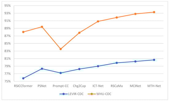
Figure 8. The comprehensive performance scores (${\mathrm{S}}_{\mathrm{m}}^{*}$) of the MTH-Net and some previous methods on the LEVIR-CDC and WHU-CDC datasets.

As shown in Table 1 and Table 2, for the IoU metric in the RSICD evaluation, the MTH-Net slightly underperformed compared to the MCINet. We speculate that although the MTH-Net adopts the same joint training strategy with the same overall loss function as that of the MCINet, the MCINet configures independent branches for the CC and CD tasks during its framework construction. While this increases the model size, it enables the MCINet to stabilize the performance through three-stage training: initial joint training, followed by separately freezing the parameters of one task branch to fine-tune the other. In contrast, our MTH-Net primarily relies on joint training and employs a shared-feature-generation architecture where both tasks utilize a common set of core processing units to enable dynamic interaction. This means that fine-tuning the CD task inevitably affects the already-optimized CC parameters, and vice versa. Although the MTH-Net still achieves higher evaluation scores than some mainstream CD methods due to the advantages of multi-task learning, this architecture limits the optimization potential for the CD task. Therefore, we conducted second-stage training through the partial fine-tuning of the pretrained MTH-Net model. Since our research focus prioritized improving the CC task performance, we froze all CC-related parameters during training and only fine-tuned the CD mask generator. The final experimental results in Table 3 demonstrate that this strategy successfully increased the model’s IoU scores by 0.4% and 2% on the LEVIR-CDC and WHU-CDC datasets, respectively, compared to the initial training. It also achieved a superior performance over the MCINet in the recall, F1-score, and IoU metrics.

Table 3. Performance comparison of the MTH-Net on RSICD tasks using the LEVIR-CDC and WHU-CDC datasets before and after fine-tuning.

Dataset	Method	Fine-Tuning	P	R	F1	IoU
LEVIR-CDC	MTH-Net	×	92.63	89.62	91.10	83.65
	MTH-Net	√	91.96	90.59	91.27	83.94
	MCINet	-	92.43	89.99	91.20	83.82
WHU-CDC	MTH-Net	×	96.27	89.16	92.58	86.18
	MTH-Net	√	96.38	90.89	93.56	87.89
	MCINet	-	96.51	90.48	93.40	87.62

Fine-tuning, specifically referring to whether the MTH-Net undergoes two-stage fine-tuning for the CD task. This process involves freezing all parameters except those of the CD mask generator, followed by retraining. In the table, P, R, and F1 represent the precision, recall, and F1-score for the change category, respectively.

4.4. Ablation Experiment

To fully evaluate the contribution of each module to the model performance, we conducted an ablation study on the LEVIR-MCI dataset and report the results for the CC task metrics, FLOPs, and batch time. The LEVIR-MCI dataset’s CD annotations cover buildings, roads, and background. This helped us gain clearer insight into the differences in the impact of CD annotations with different numbers of classes on enhancing the CC task. Additionally, it allowed us to present richer qualitative visualization results. We tested five versions by removing different modules from the MTH-Net, and the results are shown in Table 4. In the top row, MFG and CU indicate whether to use the multi-class feature generation module and the channel attention extraction unit (which performs the broadcast operation), respectively. MCA and Bi-SSM indicate whether multi-head cross-attention and bidirectional SSM blocks are used. Sp and Ti denote spatial modeling and temporal modeling, respectively. The five ablation test models are composed as follows:

Table 4. Results of ablation experiments carried out by the MTH-Net on the LEVIR-MCI dataset.

Method	MFG	Sp-Ti	MCA	Bi-SSM	CU	BLEU-4	METEOR	ROUGE-L	CIDEr-D	FLOPs (G)	Batch Time (s)
Baseline	-	-	√	√	√	65.25	40.29	75.25	137.62	16.73	58.333
${\mathrm{MTH-Net}}^1$	√	Sp	√	-	-	65.58	39.57	74.72	136.09	16.05	51.503
${\mathrm{MTH-Net}}^2$	√	Ti	-	√	-	65.07	40.21	75.23	138.47	16.60	51.037
${\mathrm{MTH-Net}}^3$ $({\mathrm{F}}_{\mathrm{dif}}^{(l)}$ removed)	√	Ti	-	√	-	64.89	39.35	74.45	137.37	15.80	50.261
${\mathrm{MTH-Net}}^4$	√	√	√	√	-	65.42	40.63	75.93	139.14	17.94	63.168
MTH-Net (EG ver.)	√	√	√	√	√	65.80	40.47	75.76	139.78	8.00	35.665
MTH-Net (JT ver.)	√	√	√	√	√	66.19	40.53	75.73	140.56	17.94	63.013
MCINet						65.93	40.30	75.55	139.05	18.31	67.100

“EG ver.” and “JT ver.” denote the explicit guidance and joint training versions, respectively. In addition, the FLOP value does not account for the language decoder part. The experimental data in the part of the Batch Time was obtained using the same GPU. The Batch Time represents the average processing time per 100 batches, with a batch size of 64. The MCINet’s data are from the reproduction experiment.

• Baseline: We undid the MFG module when setting the Baseline. That is, after adding the position embedding to the basic features of the bi-temporal image, it did not go through dynamic convolution. The multi-scale fusion feature (${\mathrm{F}}_{{\mathrm{S}}_{\mathrm{i}}}^{(l)}\in {\mathrm{R}}^{\mathrm{L}\times \mathrm{C}}$), spatial difference feature (${\mathrm{F}}_{\mathrm{dif}}^{(l)}\in {\mathrm{R}}^{\mathrm{L}\times \mathrm{C}}$), and time connection feature (${\mathrm{F}}_{\mathrm{time}}^{(l)}\in {\mathrm{R}}^{2\mathrm{L}\times \mathrm{C}}$) are no longer generated. Each temporal feature is processed by an MCA unit and a Bi-SSM block, respectively, and the CU unit is still used to extract the channel attention and fusion with the Bi-SSM block output by the broadcast operation.
• ${\mathrm{MTH-Net}}^1$: The MGF module is retained but does not output ${\mathrm{F}}_{\mathrm{t}\mathrm{i}\mathrm{m}\mathrm{e}}^{(l)}$. The Bi-SSM block for time modeling is canceled, and only the multi-scale fusion feature (${\mathrm{F}}_{{\mathrm{S}}_{\mathrm{i}}}^{(l)}$), spatial difference feature (${\mathrm{F}}_{\mathrm{dif}}^{(l)}$), and MCA unit are used for spatial modeling.
• ${\mathrm{MTH-Net}}^2$: This model also retains the MGF module, discards the use of MCA units for spatial modeling, and only uses the temporal connection feature (${\mathrm{F}}_{\mathrm{t}\mathrm{i}\mathrm{m}\mathrm{e}}^{(l)}$), spatial difference feature (${\mathrm{F}}_{\mathrm{dif}}^{(l)}$), and Bi-SSM blocks for temporal modeling. Among them, ${\mathrm{F}}_{\mathrm{t}\mathrm{i}\mathrm{m}\mathrm{e}}^{(l)}$ is the main input of the Bi-SSM block, and ${\mathrm{F}}_{\mathrm{dif}}^{(l)}$ is the input of its activation branch.
• ${\mathrm{MTH-Net}}^3$: Based on the ${\mathrm{MTH-Net}}^2$, ${\mathrm{F}}_{\mathrm{dif}}^{(l)}$ is not introduced, and only ${\mathrm{F}}_{\mathrm{t}\mathrm{i}\mathrm{m}\mathrm{e}}^{(l)}$ is used for time modeling.
• ${\mathrm{MTH-Net}}^4$: Only on the basis of the original model is the channel attention extraction unit canceled. That is, the output of the MCA unit and the Bi-SSM block is directly multiplied element by element to achieve fusion without using the broadcast mechanism.

From the experimental results, when trained on the LEVIR-MCI dataset, both the MCINet and MTH-Net models demonstrate higher BLEU-4 values than when using the LEVIR-CDC dataset. This indicates that introducing multi-category CD masks into multi-task learning exerts a beneficial impact on improving the description accuracy. The multi-category CD masks possess a higher differentiation of changing objects, providing clearer supervisory signals at the semantic level for the CC task.

The ${\mathrm{MTH-Net}}^4$ retains most of the structure of the original version of the model, and the comprehensive performance of the evaluation indicators is the best. However, because the broadcast mechanism is removed and the output features of the MCA and Bi-SSM are directly fused by element-wise multiplication, although the advantages of the MCA and Bi-SSM can be effectively utilized to some degree, their background noise will also be introduced. As a result, the discrimination accuracy of changes is reduced. Due to the complex background, multi-category target objects, and temporal characteristics of RS images, the model may identify “spurious changes” in the process of capturing changing objects due to illumination, seasons, and other factors, such as object shape changes caused by shadows and building color changes caused by lighting or photography, which may cause misjudgment. These issues have always troubled the RS image-processing fields, such as RSICC and RSICD. We retain the broadcast mechanism in the SDPN, which only takes the output of the Bi-SSM as the main propagation direction, while the MCA outputs channel weights after spatial modeling to selectively enhance the Bi-SSM output along the channel dimension. This not only makes up for the disadvantage of the insufficient utilization of channel information generated by the Bi-SSM as a state space model but also controls the range of irrelevant change noise.

The Baseline model performs on average on the overall data due to the elimination of dynamic convolutions and multi-class features in MGF. For target objects of different scales in RS images, the dynamic convolution unit can extract multi-scale features in the bi-temporal image in parallel and fuse them through a variety of different specifications of convolution kernels. This method can further enrich the representation information in the bi-temporal basic features and create favorable conditions for the subsequent change perception. Introducing spatial difference features into the SDPN can further strengthen the ability of the change perception in the core processing unit. When MCA extracts the channel attention weight, it inevitably compresses the sequence dimension, thereby losing part of the spatial information. In order to alleviate this situation, we first multiply ${\mathrm{F}}_{\mathrm{dif}}^{(l)}$ with a set of bi-temporal features (${\mathrm{F}}_{{\mathrm{S}}_{\mathrm{i}}}^{(l)}$) element by element to fully integrate the spatial difference information into the channel dimension, and we then take this group of features containing spatial difference information as the K (V) of MCA in spatial modeling and calculate the attention score with ${\mathrm{F}}_{{\mathrm{S}}_{\mathrm{i}}}^{(l)}$ as Q. The K (V) guides the model to focus on regions and objects that have changed in space and capture their dependencies. This is confirmed by the performance of the ${\mathrm{MTH-Net}}^1$, which achieved the relatively highest BLEU-4 score of the five tested versions, indicating that it generates words with high accuracy. However, it performed only average on other evaluation metrics, most likely due to the lack of a timing analysis module. Compared with static tasks such as RS image captioning (RSIC) and detection (RSID), RSICC and RSICD focus on further highlighting temporal continuity changes based on spatial positioning. We splice the bi-temporal feature (${\mathrm{F}}_{{\mathrm{S}}_{\mathrm{i}}}^{(l)}$) along the sequence dimension in chronological order and then send the 2L length (${\mathrm{F}}_{\mathrm{t}\mathrm{i}\mathrm{m}\mathrm{e}}^{(l)}\in {\mathbb{R}}^{2\mathrm{L}\times \mathrm{C}}$) into the Bi-SSM block for processing. At the same time, ${\mathrm{F}}_{\mathrm{dif}}^{(l)}$ is the activation branch input of the Bi-SSM, which will selectively modulate the output of the SSM and guide the model in effectively perceiving the time evolution trend in the sequence context. For example, words such as “narrowing” and “widening” are used to describe the changes in the same object in the bi-temporal image at different times. It can be seen that the ${\mathrm{MTH-Net}}^2$ achieved relatively high METEOR, ${\mathrm{ROUGE}}_{\mathrm{L}}$, and CIDER-D scores.

Additionally, we calculated the FLOPs and Batch Time for the MTH-Net, the representative multi-task-learning MCINet method, and five ablation test models. It can be observed that the MTH-Net (JT ver.) achieved lower FLOPs and shorter batch times than the MCINet by leveraging the shared-feature mechanism. However, while the MTH-Net (EG ver.) effectively reduces the computational complexity and batch time by decoupling the CD and CC tasks, it exhibits a slower inference time than that of several methods. It was found during training that this version’s total inference time on the validation set reached 217.78 s, substantially higher than that of the MTH-Net (JT ver.)’s 178.03 s. We speculate that this may be because using the generated masks to enhance the RSICC task first requires a downsampling operation, which could further reduce the processing efficiency as the batch size increases. When comparing the ${\mathrm{MTH-Net}}^1$ and ${\mathrm{MTH-Net}}^2$, we found that introducing ${\mathrm{F}}_{\mathrm{dif}}^{(l)}$ as an activation branch causes the Bi-SSM block to generate significantly higher FLOPs, even exceeding those of the MCA. Further experiments revealed that without introducing ${\mathrm{F}}_{\mathrm{dif}}^{(l)}$, the Bi-SSM block had lower FLOPs than the MCA, albeit with a degraded performance. However, in both scenarios, the Bi-SSM block demonstrated a faster batch time than the MCA, as confirmed by experimental data from the ${\mathrm{MTH-Net}}^3$. This situation benefitted from the hardware-friendly algorithms and selective scan mechanism of the Mamba architecture, which were better suited to our task.

4.5. Parametric Analysis

To further evaluate the intrinsic advantages of the Mamba–Transformer hybrid architecture encoder, we conducted a series of controlled experiments focusing on model depth and architectural comparisons to investigate the reasons for the performance improvement. The experimental results are shown in Table 5.

Table 5. The performance of the MTH-Net with different numbers of attention encoding layers and its comparison with the Transformer and Mamba encoder methods in the LEVIR-MCI database.

Method	Encoder Type	Number of Encoder Layers	BLEU-4	METEOR	ROUGE-L	CIDEr-D	${\mathbf{S}}_{\mathbf{m}}^{*}$	Param. (M)
Chg2Cap [35]	Transformer	-	63.90	39.88	74.14	135.05	78.24	285.50
RSCaMa [17]	Mamba	-	64.86	40.79	75.48	138.38	79.88	176.90
MTH-Net	M-T hybrid	2	65.94	40.08	75.37	138.43	79.96	172.15
MTH-Net		4	64.66	40.29	75.57	137.72	79.56	323.16
MTH-Net		3	66.19	40.53	75.73	140.56	80.75	247.65

4.5.1. Model Depth Analysis

The results indicate that the number of attention encoder layers is a critical hyperparameter. Our model achieved a peak performance with three layers, obtaining the highest BLEU-4 and ${\mathrm{S}}_{\mathrm{m}}^{*}$. When the number of layers is reduced to two, the model’s capacity may be insufficient for complex change reasoning, leading to performance degradation. Conversely, increasing the number of layers to four, which increases the parameter count, results in lower evaluation scores, suggesting potential overfitting. We speculate that increasing the depth beyond three layers may not introduce additional meaningful representations. Instead, it may cause the model to learn redundant features from the training dataset, impairing the generalization capability. Furthermore, as the network depth increases, limited hardware resources face greater optimization challenges, which may also contribute to performance limitations.

4.5.2. Analysis of Hybrid Architecture

In experiments validating the effectiveness of the M-T hybrid architecture, we used a set of RSICC methods based on Transformer and Mamba architecture encoders as baseline comparison models, specifically Chg2Cap and RSCaMa. With a comparable or lower number of parameters, the MTH-Net achieved a 3.2% improvement in the ${\mathrm{S}}_{\mathrm{m}}^{*}$ over Chg2Cap and a 1.7% higher BLEU-4 compared to RSCaMa. This indicates that the intrinsic advantage of the hybrid architecture stems from the effective synergy and complementary strengths achieved through mechanisms such as broadcasting and selective modulation, rather than merely increasing the model capacity.

4.6. Qualitative Visualization

We used the pretrained models generated by the MTH-Net and Baseline on the LEVIR-MCI and WHU-CDC datasets to make predictions on the test set, and we present some of the prediction results, as shown in Figure 9 and Figure 10. The results visually compare the differences between the change masks and captions predicted by the Baseline and MTH-Net and the true annotations. Among them, most of the prediction results selected by WHU-CDC were dominated by urban or suburban changes, while LEVIR-MCI included backgrounds such as forests and roads, to present the adaptability of the MTH-Net and Baseline to complex scenes.

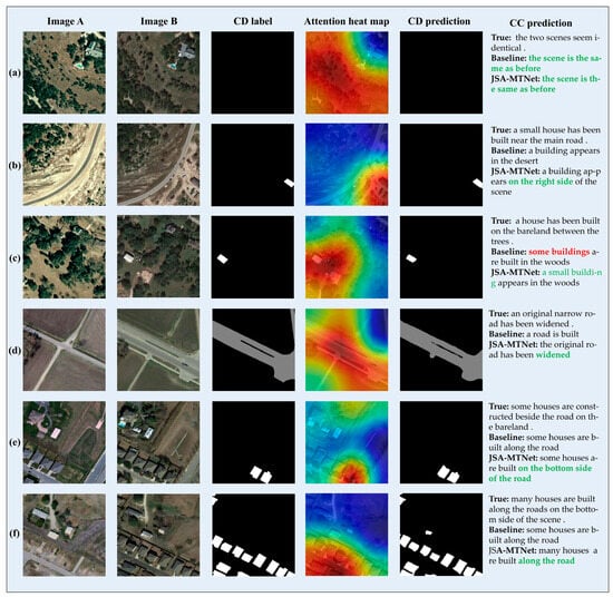
Figure 9. The visualization of the partial prediction results from the MTH-Net on the LEVIR-MCI dataset is shown in the figure, which includes, from left to right, the bi-temporal images from the dataset, CD mask labels, attention heatmaps generated by the SDPN, change detection masks produced by the MTH-Net, and predicted descriptive sentences. The red text in the figure indicates incorrect titles, while the green text indicates valid titles.

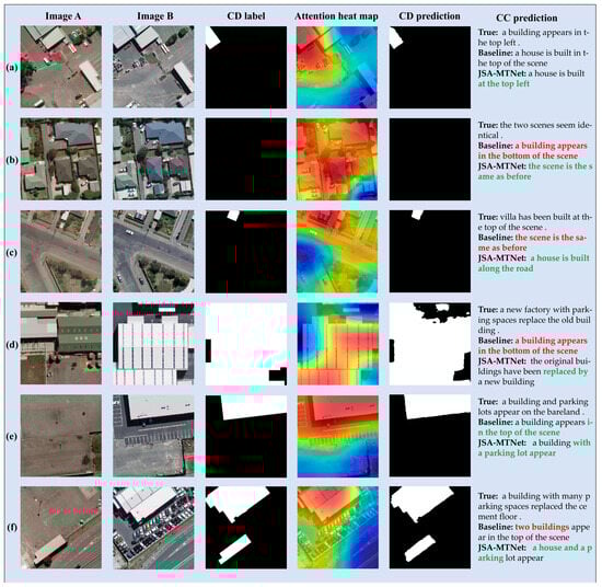
Figure 10. This figure visualizes partial prediction results of our MTH-Net on the WHU-CDC dataset. The arrangement of elements follows the same layout as that in Figure 9.

The bi-temporal image in Figure 9a contains many different types of target objects, such as buildings, small targets, and forests, and the two methods can give the correct discrimination of “unchanged”, which shows the advantages of the multi-task learning method. The CD and CC tasks can improve the anti-noise performance of the model as much as possible through the implicit mutual guidance. The collaboration between pixel-level and semantic-level tasks can effectively prevent misjudgments caused by irrelevant targets, such as changes in tree colors and shadow areas due to factors such as seasons and lighting. In Figure 10b, the Baseline misjudges due to the color of the house, while the MTH-Net effectively filtered irrelevant changes because the channel dimension through the spatial modeling branch contains color, edge texture, and other change type information, which is integrated into the output of the temporal modeling branch in the form of broadcast, improving the ability of the model to discriminate the change in fine-grained features of the target.

The advantages of spatial modeling are mainly reflected in spatial object localization and dependency capture. As shown in Figure 9b and Figure 10a, the MTH-Net locates the position of the target object and can form more accurate descriptive sentences using phrases such as “top left” and “on the right side”. In Figure 9c, it can be seen that the model correctly judged the number of changing objects, not “some” but “a”. Compared with the Baseline, the MTH-Net introduces the spatial difference feature into the spatial modeling to guide the attention to focus on the correct change area. In Figure 10f, the result of the change mask also reflects that the model correctly determined the number of change objects in the space, and the category of change objects is reflected in the caption, which includes “house” and “parking”. Figure 9f and Figure 10c show the model’s ability to capture the dependence between spatial objects. The spatial modeling branch realizes effective global correlation calculations for various types of target objects in the space through the cross-attention mechanism and enables the model to describe the relationship between objects with prepositions such as “along” and “side of”. For the Figure 9e example, the model uses “bottom” to accurately determine the positions of the “house” and “road” when describing their relationship.

Figure 10d shows the effect of the time modeling branch. The two temporal features “before” and “after” are composed into a splicing sequence in time order, and then context modeling from the time dimension effectively captures the time continuity change, which can be reflected by words such as “appear” and “replace” in the descriptive statement. Figure 9d and Figure 10e demonstrate the advantages of joint modeling to bi-temporal sequences from both the temporal and spatial dimensions. In Figure 9d, the change of “road” through spatial modeling is located, and the time analysis further judged that “the original road has been widened”. In Figure 10e, the model identifies the change category as “appear” and uses “with” to express the dependency between “building” and “parking”.

5. Conclusions

Previous RSICC methods often used mainstream architectures or their variants to construct the primary components of encoders. These methods may encounter performance bottlenecks due to their own working mechanisms and overall structural characteristics. In this study, we constructed a Siamese network with a symmetric architecture named the MTH-Net. It forms a systematic encoder structure that integrates feature machining and parallel feature handling through MGF and the SDPN. According to the characteristics of the two mainstream models, we respectively performed corresponding time and space modeling tasks on suitable features and achieved channel-level fusion through the broadcast mechanism to leverage their complementary advantages. To alleviate the computational burden of multi-task learning, the MTH-Net employs a feature-sharing mechanism. This allows different tasks to share a main network, reducing the computational cost and enhancing inter-task interaction during parameter optimization. Additionally, we constructed two multi-task collaborative methods based on the MTH-Net: joint training based on the total loss function, and CC enhancement explicitly guided by the generated CD masks. Experimental results demonstrate that both methods achieved performance improvements while also validating the potential of symmetric architecture frameworks for image change analysis.

For future research, we will focus on addressing the limitations. Due to adopting the multi-task feature-sharing mechanism, the MTH-Net cannot achieve an effective three-stage training process like other multi-task methods, such as the MCINet. The Mamba–Transformer-integrated architecture within the SDPN employs a parallel-processing-then-fusion strategy, which may lead to slight overfitting. We expect to find solutions to these issues in the future. Additionally, we plan to leverage the powerful capabilities of existing large-scale model technologies to more effectively generate CC task labels for other remote sensing image datasets, thereby constructing specialized RSICC datasets tailored to specific scenarios. This will facilitate further exploration of the generalization capability of symmetric Siamese network-based RSICC methods.

References

- Tewkesbury, A.P.; Comber, A.J.; Tate, N.J.; Lamb, A.; Fisher, P.F. A critical synthesis of remotely sensed optical image change detection techniques. Remote Sens. Environ. 2015, 160, 1–14. [Google Scholar] [CrossRef]
- Liu, Y.; Pang, C.; Zhan, Z.; Zhang, X.; Yang, X. Building change detection for remote sensing images using a dual-task constrained deep siamese convolutional network model. IEEE Geosci. Remote Sens. Lett. 2020, 18, 811–815. [Google Scholar] [CrossRef]
- Malila, W.A. Change vector analysis: An approach for detecting forest changes with Landsat. In Proceedings of the LARS Symposia, West Lafayett, ID, USA, 3–6 June 1980; p. 385. [Google Scholar]
- Tang, X.; Zhang, H.; Mou, L.; Liu, F.; Zhang, X.; Zhu, X.X.; Jiao, L. An unsupervised remote sensing change detection method based on multiscale graph convolutional network and metric learning. IEEE Trans. Geosci. Remote Sens. 2021, 60, 5609715. [Google Scholar] [CrossRef]
- Chouaf, S.; Hoxha, G.; Smara, Y.; Melgani, F. Captioning changes in bi-temporal remote sensing images. In Proceedings of the 2021 IEEE International Geoscience and Remote Sensing Symposium IGARSS, Brussels, Belgium, 11–16 July 2021; pp. 2891–2894. [Google Scholar]
- Liu, C.; Zhao, R.; Chen, H.; Zou, Z.; Shi, Z. Remote sensing image change captioning with dual-branch transformers: A new method and a large scale dataset. IEEE Trans. Geosci. Remote Sens. 2022, 60, 5633520. [Google Scholar] [CrossRef]
- Li, Z.; Tang, C.; Wang, L.; Zomaya, A.Y. Remote sensing change detection via temporal feature interaction and guided refinement. IEEE Trans. Geosci. Remote Sens. 2022, 60, 5628711. [Google Scholar] [CrossRef]
- Chen, H.; Qi, Z.; Shi, Z. Remote sensing image change detection with transformers. IEEE Trans. Geosci. Remote Sens. 2021, 60, 5607514. [Google Scholar] [CrossRef]
- Peng, X.; Zhong, R.; Li, Z.; Li, Q. Optical remote sensing image change detection based on attention mechanism and image difference. IEEE Trans. Geosci. Remote Sens. 2020, 59, 7296–7307. [Google Scholar] [CrossRef]
- Saha, S.; Bovolo, F.; Bruzzone, L. Unsupervised deep change vector analysis for multiple-change detection in VHR images. IEEE Trans. Geosci. Remote Sens. 2019, 57, 3677–3693. [Google Scholar] [CrossRef]
- Hoxha, G.; Chouaf, S.; Melgani, F.; Smara, Y. Change captioning: A new paradigm for multitemporal remote sensing image analysis. IEEE Trans. Geosci. Remote Sens. 2022, 60, 5627414. [Google Scholar] [CrossRef]
- He, K.; Zhang, X.; Ren, S.; Sun, J. Deep residual learning for image recognition. In Proceedings of the IEEE Conference on Computer Vision and Pattern Recognition, Las Vegas, NV, USA, 27–30 June 2016; pp. 770–778. [Google Scholar]
- Liu, C.; Zhao, R.; Chen, J.; Qi, Z.; Zou, Z.; Shi, Z. A decoupling paradigm with prompt learning for remote sensing image change captioning. IEEE Trans. Geosci. Remote Sens. 2023, 61, 5622018. [Google Scholar] [CrossRef]
- Liu, C.; Yang, J.; Qi, Z.; Zou, Z.; Shi, Z. Progressive scale-aware network for remote sensing image change captioning. In Proceedings of the IGARSS 2023—2023 IEEE International Geoscience and Remote Sensing Symposium, Pasadena, CA, USA, 16–21 July 2023; pp. 6668–6671. [Google Scholar]
- Cai, C.; Wang, Y.; Yap, K.-H. Interactive change-aware transformer network for remote sensing image change captioning. Remote Sens. 2023, 15, 5611. [Google Scholar] [CrossRef]
- Sun, D.; Bao, Y.; Liu, J.; Cao, X. A lightweight sparse focus transformer for remote sensing image change captioning. IEEE J. Sel. Top. Appl. Earth Obs. Remote Sens. 2024, 17, 18727–18738. [Google Scholar] [CrossRef]
- Liu, C.; Chen, K.; Chen, B.; Zhang, H.; Zou, Z.; Shi, Z. Rscama: Remote sensing image change captioning with state space model. IEEE Geosci. Remote Sens. Lett. 2024, 21, 6010405. [Google Scholar] [CrossRef]
- Liu, C.; Chen, K.; Zhang, H.; Qi, Z.; Zou, Z.; Shi, Z. Change-agent: Towards interactive comprehensive remote sensing change interpretation and analysis. IEEE Trans. Geosci. Remote Sens. 2024, 62, 5635616. [Google Scholar] [CrossRef]
- Xie, E.; Wang, W.; Yu, Z.; Anandkumar, A.; Alvarez, J.M.; Luo, P. SegFormer: Simple and efficient design for semantic segmentation with transformers. Adv. Neural Inf. Process. Syst. 2021, 34, 12077–12090. [Google Scholar]
- Dosovitskiy, A.; Beyer, L.; Kolesnikov, A.; Weissenborn, D.; Zhai, X.; Unterthiner, T.; Dehghani, M.; Minderer, M.; Heigold, G.; Gelly, S. An image is worth 16x16 words: Transformers for image recognition at scale. arXiv 2020, arXiv:2010.11929. [Google Scholar]
- Wu, C.; Zhang, L.; Du, B.; Chen, H.; Wang, J.; Zhong, H. UNet-Like Remote Sensing Change Detection: A review of current models and research directions. IEEE Geosci. Remote Sens. Mag. 2024, 12, 305–334. [Google Scholar] [CrossRef]
- Vaswani, A.; Shazeer, N.; Parmar, N.; Uszkoreit, J.; Jones, L.; Gomez, A.N.; Kaiser, Ł.; Polosukhin, I. Attention is all you need. In Proceedings of the 31st Conference on Neural Information Processing Systems (NIPS 2017), Long Beach, CA, USA, 4–9 December 2017; Volume 30. [Google Scholar]
- Ma, C.; Lv, X.; Xie, Q.; Luo, Z. Cross-layer Attention Enhanced Remote Sensing Image Change Captioning via Mamba-Transformer Interaction. In Proceedings of the 2025 6th International Conference on Geology, Mapping and Remote Sensing (ICGMRS), Wuhan, China, 25–27 April 2025; pp. 245–248. [Google Scholar]
- Jiang, A.; Chen, H.; Chen, Z.; Ye, J.; Wang, M. Multi-dimensional Visual Prompt Enhanced Image Restoration via Mamba-Transformer Aggregation. arXiv 2024, arXiv:2412.15845. [Google Scholar]
- Zhu, L.; Liao, B.; Zhang, Q.; Wang, X.; Liu, W.; Wang, X. Vision Mamba: Efficient Visual Representation Learning with Bidirectional State Space Model. arXiv 2024. [Google Scholar] [CrossRef]
- Gu, A.; Dao, T. Mamba: Linear-time sequence modeling with selective state spaces. arXiv 2023, arXiv:2312.00752. [Google Scholar] [CrossRef]
- Liu, R.; Li, K.; Song, J.; Sun, D.; Cao, X. Mv-cc: Mask enhanced video model for remote sensing change caption. arXiv 2024, arXiv:2410.23946. [Google Scholar] [CrossRef]
- Papineni, K.; Roukos, S.; Ward, T.; Zhu, W.-J. Bleu: A method for automatic evaluation of machine translation. In Proceedings of the 40th Annual Meeting of the Association for Computational Linguistics, Philadelphia, PA, USA, 7–12 July 2002; pp. 311–318. [Google Scholar]
- Banerjee, S.; Lavie, A. METEOR: An automatic metric for MT evaluation with improved correlation with human judgments. In Proceedings of the ACL Workshop on Intrinsic and Extrinsic Evaluation Measures for Machine Translation and/or Summarization, Ann Arbor, MI, USA, 29 June 2005; pp. 65–72. [Google Scholar]
- Lin, C.-Y. Rouge: A package for automatic evaluation of summaries. In Proceedings of the Text Summarization Branches Out, Barcelona, Spain, 25–26 July 2004; pp. 74–81. [Google Scholar]
- Vedantam, R.; Lawrence Zitnick, C.; Parikh, D. Cider: Consensus-based image description evaluation. In Proceedings of the IEEE Conference on Computer Vision and Pattern Recognition, Boston, MA, USA, 7–12 June 2015; pp. 4566–4575. [Google Scholar]
- Shi, J.; Zhang, M.; Hou, Y.; Zhi, R.; Liu, J. A multi-task network and two large scale datasets for change detection and captioning in remote sensing images. IEEE Trans. Geosci. Remote Sens. 2024, 62, 2007017. [Google Scholar] [CrossRef]
- Ji, S.; Wei, S.; Lu, M. Fully convolutional networks for multisource building extraction from an open aerial and satellite imagery data set. IEEE Trans. Geosci. Remote Sens. 2018, 57, 574–586. [Google Scholar] [CrossRef]
- Park, D.H.; Darrell, T.; Rohrbach, A. Robust change captioning. In Proceedings of the IEEE/CVF International Conference on Computer Vision, Seoul, Republic of Korea, 27 October–2 November 2019; pp. 4624–4633. [Google Scholar]
- Chang, S.; Ghamisi, P. Changes to captions: An attentive network for remote sensing change captioning. IEEE Trans. Image Process. 2023, 32, 6047–6060. [Google Scholar] [CrossRef]
- Ye, Y.; Wang, M.; Zhou, L.; Lei, G.; Fan, J.; Qin, Y. Adjacent-level feature cross-fusion with 3-D CNN for remote sensing image change detection. IEEE Trans. Geosci. Remote Sens. 2023, 61, 5618214. [Google Scholar] [CrossRef]
- Han, C.; Wu, C.; Guo, H.; Hu, M.; Chen, H. HANet: A hierarchical attention network for change detection with bitemporal very-high-resolution remote sensing images. IEEE J. Sel. Top. Appl. Earth Obs. Remote Sens. 2023, 16, 3867–3878. [Google Scholar] [CrossRef]
- Noman, M.; Fiaz, M.; Cholakkal, H.; Khan, S.; Khan, F.S. ELGC-Net: Efficient local–global context aggregation for remote sensing change detection. IEEE Trans. Geosci. Remote Sens. 2024, 62, 4701611. [Google Scholar] [CrossRef]
- Zhang, H.; Teng, Y.; Li, H.; Wang, Z. STRobustNet: Efficient Change Detection via Spatial-Temporal Robust Representations in Remote Sensing. IEEE Trans. Geosci. Remote Sens. 2025, 63, 5612215. [Google Scholar] [CrossRef]
Disclaimer/Publisher’s Note: The statements, opinions and data contained in all publications are solely those of the individual author(s) and contributor(s) and not of MDPI and/or the editor(s). MDPI and/or the editor(s) disclaim responsibility for any injury to people or property resulting from any ideas, methods, instructions or products referred to in the content. |
© 2025 by the authors. Licensee MDPI, Basel, Switzerland. This article is an open access article distributed under the terms and conditions of the Creative Commons Attribution (CC BY) license (https://creativecommons.org/licenses/by/4.0/).