Kramers Degeneracy and Spin Inversion in a Lateral Quantum Dot


1
Kirensky Institute of Physics, Federal Research Center KSC Siberian Branch, Russian Academy of Sciences, 660036 Krasnoyarsk, Russia
2
Departament de Física, Universitat de les Illes Balears, E-07122 Palma de Mallorca, Spain
3
Bogoliubov Laboratory of Theoretical Physics, Joint Institute for Nuclear Research, 141980 Dubna, Russia
4
Faculty of Natural and Engineering Science, Dubna State University, 141982 Dubna, Russia
*
Author to whom correspondence should be addressed.
Symmetry 2020, 12(12), 2043; https://doi.org/10.3390/sym12122043
Submission received: 19 October 2020
/
Revised: 29 November 2020
/
Accepted: 8 December 2020
/
Published: 10 December 2020
(This article belongs to the Special Issue Symmetry and Mesoscopic Physics)
Abstract
:We show that the axial symmetry of the Bychkov–Rashba interaction can be exploited to produce electron spin-flip in a circular quantum dot, without lifting the time reversal symmetry. In order to elucidate this effect, we consider ballistic electron transmission through a two-dimensional circular billiard coupled to two one-dimensional electrodes. Using the tight-binding approximation, we derive the scattering matrix and the effective Hamiltonian for the considered system. Within this approach, we found the conditions for the optimal realization of this effect in the transport properties of the quantum dot. Numerical analysis of the system, extended to the case of two-dimensional electrodes, confirms our findings. The relatively strong quantization of the quantum dot can make this effect robust against the temperature effects.
1. Introduction
Spin-polarized transport in semiconductor nanostructures attracts a continuous experimental and theoretical attention due to great interests for both basic research and device applications (see for a review [1,2,3]). Indeed, apart fundamental aspects related to the origin of spin current in nanosystems, the inversion of spin polarization is necessary, for example, for operation of spin-based logic elements. The inversion of spin polarization can be achieved in an external AC field with the aid of the electron spin resonance (see, for example, [4]), or by the lifting the spin degeneracy by means of a magnetic field that induces the Zeeman splitting (e.g., [5]). The spin currents can be inverted also by mechanical strain of a silicene [6]. Periodically rippled graphene can as well invert the polarized spin current, by changing the electron flow direction through the system [7].
One of the main requirements for device operability is the efficient manipulation of spin-polarized currents in a semiconductor structure. An additional condition for device applications is that a polarized current should be generated by means of all-electrical methods. In particular, a remarkable progress has been achieved in all-electrical injection from ferromagnetic contacts [8,9] and (Ga,Mn)As [10]. Alternatively to the injection, a spin-orbit interaction (SOI) present in semiconductors provides a natural mechanism to manipulate the spin (e.g., [11,12,13,14]). In particular, the electrical field, caused by the structure inversion asymmetry of the heterostructure, gives rise to the Bychkov–Rashba term [15,16]. The strength of this interaction can be controlled by means of an applied electric field [17,18,19]. It should be mentioned that the Rashba interaction is one of the basic ingredients in the physics of Majorana fermions [20,21,22]. This physics is based on two superconducting electrodes electrically connected to a semiconductor nanowire with strong Rashba coupling, and a uniform magnetic field. The explosive activity in this direction includes among many proposals as well the use of high-temperature cuprate superconductors [23] and exotic pairs of parafermions without magnetic field [24] to create Majorana zero modes for quantum computing applications (e.g., [25,26,27]).
Several proposals rely on the SOI as the basic mechanism to achieve a spin filtering effect in low-dimensional semiconductor structures [28,29,30,31]. In fact, it might allow for an all-electrical spin-polarized current generation. The relatively small energy scale, produced by the SOI, presents, however, a major obstacle for technological applications. Indeed, the spin splitting induced by the SOI in typical semiconductor alloys can reach a few meV [17,18]. This scale stipulates certain restrictions on the choice of nanosystems that would be enabled to overcome the impact of thermal effects. It is well known that wide gap semiconductors (e.g., GaAs) possess a relatively weak spin-orbit interaction. In contrast, narrow gap semiconductors own strong spin-orbit couplings as well as g factors. These two factors guide the choice of most favorable materials, especially, in view of the Majorana physics. The latter question is, however, beyond the scope of the present paper, and we leave this problem for future. The main result of the present paper is that the symmetry of a circular quantum dot can be used to obtain the robust mechanism to inverse z-component of spin-polarized current for non-magnetic metallic contacts.
2. Symmetry of Rashba SOI
It is well known that the invariance of the SOI with respect to the time-reverse operation leads to the Kramers degeneracy (e.g., [32]). Therefore, any system, where the SOI is the only spin-dependent term, will exhibit this two-fold degeneracy. Explicitly, the time reversal symmetry is obtained by inverting both spin and momentum operators. The resulting states, although degenerated in energy, are distinguished by an opposite orbital motion and an opposite spin orientation.
To employ this fundamental feature, we consider a two-dimensional (2D) semiconductor quantum dot (QD) with a circular confinement and the Rashba spin-orbit interaction. In the effective mass approximation for the conduction band, the Hamiltonian can be written as , with the single-particle Hamiltonian taken in the form
where is the electron effective mass and is an external rotationally symmetric potential. We consider the limit of the weak Coulomb interaction, when the external potential dominates in electron properties (e.g., [33]). The Bychkov–Rashba interaction has the form: . The strength parameter depends strongly on the material, reaching its maximum value for narrow gap III-V semiconductor alloys. For instance, typical values of = 10–40 meV × nm have been experimentally determined for different InAs-based structures [28,29,34]. An important feature is that the Bychkov–Rashba interaction preserves the axial symmetry, i.e., , where . Therefore, the full Hamiltonian obeys the conservation law .
In the dimensionless cylindrical coordinates and the Hamiltonian (1) takes the form
Here , is the Laplace operator, and the parameter d is a characteristic length in our system. Since the eigenstates of the Hamiltonian (2) are eigenstates of the operator, they can be expressed in the following form
where and stand for radial and the angular momentum quantum numbers, respectively. To simplify the eigenvalue problem, we represent the wavefunction (3) as a formal series with respect to the strength of the spin-orbit interaction
At the wavefunction is the radial part of the Shrödinger equation solution without the spin-orbit interaction
We recall that the energy scale, produced by the effective external potential , is larger than that produced by the spin-orbit interaction (cf [35]). Therefore, it is enough to consider the expansion of the wavefunction (4) up to the first order with the respect to the strength parameter. As a result, we obtain two differential equations for the coefficients , at :
The trivial solution of Equation (6) is , while we obtain to hold true Equation (7). Thus, the approximate eigenfunctions of the Hamiltonian (2) to the first order in can be written in the form
Below we will use this function to find the optimal conditions for the electron spin-flip phenomenon in the QD.
3. Effective Hamiltonian Model
To analyze transport properties of the circular QD we employ the effective Hamiltonian method [36,37]. According to this method, the scattering system is described by the Hamiltonian that contains the structure with discrete spectrum (our QD), the continuum with the external scattering states (external electrodes), and the interaction between continuum states with QD’s eigenstates. Evidently, once the system is opened, the discrete states of QD’s own the widths, i.e., they transform to resonance states. The main object in such an investigation is the scattering matrix that describes the relation between the amplitudes of incoming states from electrodes and the amplitudes of the reflected states from, or transmitted through the structure into electrodes.
One of the efficient approaches to reach reliable numerical results on ballistic transport through mesoscopic system is based on the tight-binding model. Following [38] we model the scattering system as a two-dimensional billiard with two attached 1D electrodes in the tight-binding representation (see details in Appendix A). In this case, the scattering matrix that describes scattering from a channel to a channel C takes the form
Here, – the wave function of a semi-infinite long electrodes (without the SOI) at the contact point; E is the electron energy in the electrode in the 1D tight-binding model. The matrix is defined as , while the effective Hamiltonian has form
Here, the coefficients
are the normalized eigenfunctions , corresponding to the eigenvalue of our structure; —the coordinate of C-th electrode junction (see Figure A1 and discussion around it in Appendix A). Note, that the index C denotes the electrode and as well the spin orientation.
Assuming a weak coupling of our structure with the external electrodes, let us consider a pair of degenerate levels with energy , i.e., near the energy E of a scattering electron. We assume also a strong confinement potential , that allows the neglecting of resonance overlapping for the open system. As discussed above, the pair of corresponding eigenfunctions are time conjugated: , where is the time-reverse operator. As a result, the following relations take place
From this property it follows immediately that the effective Hamiltonian (10) is a diagonal matrix due to the orthogonality condition . Consequently, we obtain for the S-matrix elements between two electrodes the following definitions:
where
Here, we introduce the parameter
The resonant condition arises at the electron energy
when the factor (17) reaches its maximal value . Hereafter, we assume that the ballistic transport occurs at the resonance energy (19). From Equations (13)–(16) it follows that
There are a few remarks in order. First, it should be noted that Equations (20)–(22) lead us to the fact that at the transport through our system from electrode to c the spin polarization is
This result is in the agreement with the statement that a nonzero spin polarization in system with the SOI cannot occur if there is only one open channel in electrodes [39,40].
Second, from Equation (20) it follows that the reflection coefficient with the spin-flip is always zero. The reflection coefficient without the spin-flip can be rewritten as
Finally, without loss of generality, we assume the equal coupling of the QD’s states to both electrodes (1 and 2). As a result, taking into account the definition (18), we have
Evidently, at the resonance energy (19) the reflection (23) becomes zero, and, consequently, we obtain for the S-matrix
with matrix
From the unitarity of S matrix it follows that . The spin-orbit interaction converts a two-component spinor into another two-component spinor. In particular, it could change the incoming spin up electron state to the outgoing spin down electron state and vice versa. Consequently, to reach the ideal electron spin-flip phenomenon we require that the direct scattering matrix elements (non-spin-flip components) should be equal zero: . From Equations (13) and (16) it follows that this requirement holds if the following relation takes place for the eigenstates of our QD:
To see the consequences of this relation for our system, we apply this condition to the eigenstates of the QD of the radius R: , [see Equation (3)]. In the tight-binding approximation the point is located just before the quantum point contact (QPC) between the QD and the electrode (see Figure A1). At the QPC , and the radial wave function or takes the form at :
Here a small quantity is the distance between lattice sites. Taking into account that at the Dirichlet boundary condition (a closed QD), we obtain:
(prime denotes derivative over R). As a result, the condition (27) takes the form
that leads us to the following equations:
For the approximate eigenfunction (8) we obtain the condition , resolving Equation (31). Among solutions of Equation (32) there is one which is common for all possible states with the quantum number j. In other words, an electron with the spin up (down), injected from one electrode to the QD, exits from the opposite electrode with the spin down (up). Thus, by altering either the spin-orbit strength or the QD’s radius R within the condition , we obtain the spin-flip transmission through our structure.
To illuminate this analytical solution, we consider the simplest quantum well potential of the form . The solution of the eigenvalue problem for this potential provides the radial wavefunctions and in terms of the Bessel functions (e.g., [41]). In this case, the Dirichlet boundary condition for the wavefunction (3) yields the equation
that defines the energy spectrum . Here, is the Bessel functions, and the parameter has the following structure
The application of Equation (31) leads to the transcendental equation
Plus or minus sign here are opposite to signs of -derivatives. In the case of the ideal spin-flip process the numerical solution of the transcendental Equation (35) for several lowest eigenvalues with quantum numbers j and n gives (see Table 1). Please note that the transport properties could be affected at the interface between the 1D lead and the 2D QD. However, the use of the QPC restricts the number of open channels between the electrode and the QD [42]. Consequently, we belief that our results will be valid for a realistic situation as well. To confirm our findings, we consider a 2D case below.
4. The 2D Model
The results, obtained with the aid of the one-dimension electrodes, serve to illustrate the basic principles of the spin-flip at the transmission through the QD. To elucidate these principles we have considered the particular situation, when direct transmission matrix elements were equal zero. In this section, to demonstrated the vitality and the validity of our findings we consider the 2D structure depicted in Figure 1. The QD is modelled by a constant potential (gray) with the SOI included. The ballistic electrons, propagating from one electrode to another, tunnel to the QD through the thin potential shell (dark gray). On the thin lines the Dirichlet boundary conditions are imposed. All electrodes have equal width d, while the circular QD has the radius .
We perform numerical calculations in the framework of the tight-binding approach on the square lattice ( and are 2D vectors of elementary translations with length in x and y direction, —lattice constant, and —integers). In the tight-binding approximation the system Hamiltonian (1) has the following form
Here, we use the following notations: , ; the indices stand for nearest neighbor sites n and m. We solve the Schrödinger equation in a discretized space, according to the method developed by Ando [43]. Examples of numerical treatment of quantum billiards within this approach can be found, for example, in Refs. [44,45]. In our calculations the electrode width ; while dimensionless units are defined as , where the characteristic length of the device d was chosen as the unit length. In these units the energy range corresponds to one transverse mode in all contacts.
Figure 2 displays the numerical results for the direct process as a function of the electron energy and the strength of the Rashba interaction. The results are in a good agreement with those that have been obtained from the condition (35) (see Table 1).
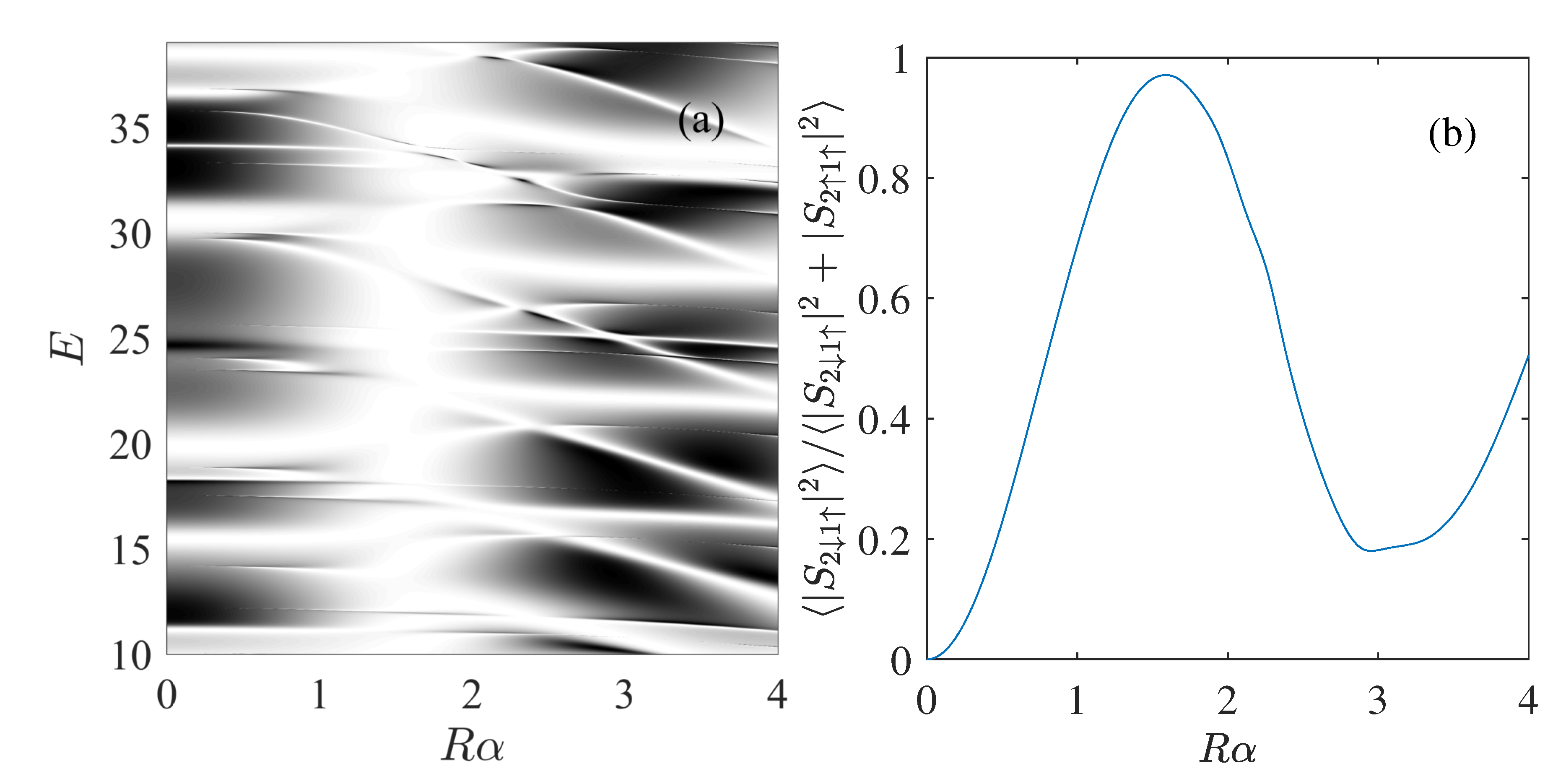
It is noteworthy that the approximate condition is unique in that there is no dependence neither on the electron energy, nor on the spin of the electron state. In other words, it can be fulfilled for a set of QD’s electron states even at large opening of the QD. To model this case (a resonance overlapping regime), we remove the potential barrier between the QD and the electrodes. Indeed, the direct spin transmission is suppressed strongly near (see Figure 3a). In this case, the spin-flip process, averaged over energy (available at the one channel transport), becomes a dominant phenomenon, reaching about ∼97% of the efficiency (see Figure 3b). In other words, the thermal effects affect only slightly the spin-flip process even in the regime of the large opening of the QD.
Larger the dot radius lesser the spin-orbit strength is required to hold the condition . However, with the increase of the dot radius the spacing between levels becomes smaller. Note, that in principle, QD levels will be affected by the coupling as well. In fact, they will be shifted with respect to those of the closed QD, especially, in the case of a strong electron-electron interaction [46]. Therefore, the discussed effect is most probable in a narrow gap semiconductor QD with a strong confinement potential and at the weak coupling regime. In this case, the resonance states will be well separated from each to other.
However, as discussed above, the overlapping of resonances and the thermal smearing decrease the efficiency of the spin-flip phenomenon as well. To evaluate the energy scaling we transform the equation in dimensional units: nm eV. In the case of InAs = 40 meV nm with the desired QD radius should be 80 nm. For the QD’ radius 100 nm the spacing between lowest levels is of the order 0.8 meV. The temperature smearing will be significant if . In other words, our device could operate with efficiency at , which is far from the typical temperature values ∼100 mK for single-electron tunneling spectroscopy experiments (see, for example, the textbook [42]).
5. Summary
We suggest the mechanism of the z-component spin inversion with the aid of the circular lateral QD that symmetrically coupled to two electrodes. The effective confinement potential of the QD consists of the circular potential well. From our analysis of the ballistic electron transport through the QD with the Rashba SOI, it follows the Kramers degeneracy of the QD levels could lead to the destructive interference of the direct () spin scattering process, while producing the spin-flip phenomenon. We found that the optimal conditions for the realization of the perfect spin-flip processes is subject to the condition . In fact, this condition depends quite weakly on the particular choice of the quantum level. We found that this effect is robust for the QD’s states at the temperature less than 9 K.
Author Contributions
Software, investigation, writing–original draft preparation, K.P.; investigation, methodology, visualization, A.P.; conceptualization, validation, investigation, writing–review and editing, supervision, R.N. All authors have read and agreed to the published version of the manuscript.
Funding
This research received no external funding.
Acknowledgments
This research has been supported partially by the guest program of The University of Illes Balears.
Conflicts of Interest
The authors declare no conflict of interest.
Appendix A. Derivation of Effective Hamiltonian on 2D Square Lattice
The Hamiltonian of our scattering system can be presented as follows:
where the Hamiltonian consists of three terms: two electrodes or with continuous spectra and a closed substructure with a discrete spectrum:
The corresponding eigenstates are normalized:
The operator connects the closed substructure with electrodes (). The stationary Shrödinger equation for the Hamiltonian reads as
while we are interested in the solution for the total Hamiltonian (A1)
For the energy E different from the eigenvalue of the closed substructure we can define the operator . Consequently, if the outgoing wave boundary condition is adopted, we can transform Equation (A6) to the Lippmann-Schwinger equation
The formal solution of this equation reads as
Following Refs. [36,37], with the aid of the basis states (A3) we construct projector operators for each term in the Hamiltonian (A2):
with the properties
By means of the projection operators the Lippmann-Schwinger Equation (A8) transforms to the following form
Here, each block of the matrix representation of the operator (A14) has the following structure
Our closed substructure is subjected to the Dirichlet boundary conditions on junction with electrodes, i.e., the following condition takes place. In other words, the operator does not affect the structure of the isolated subsystem. As a result, we have
Another reasonable assumption is the absence of the direct connection between electrodes:
Taking into account the above arguments, we transform the Lippmann-Schwinger Equation (A14) to the form
Considering the initial state in the form
we present the scattering state as
defining the scattering matrix elements
To get to the heart of the problem, let us consider, for example, the second equation from (A18), and corresponding wavefunctions , from Equation (A20):
Multiplying the both sides of Equation (A22) by , we obtain
with the following definition of the effective Hamiltonian
The eigenstates of form the natural basis for the effective Hamiltonian. Taking into account this fact, we obtain by means of Equation (A23) the following system
Here, the matrix elements have the following structure
where the matrix elements of operator are
Using the definition of (A2), we can write
To obtain the matrix elements we make the transformation to the tight-binding representation by inserting the resolution of identity into the definition:
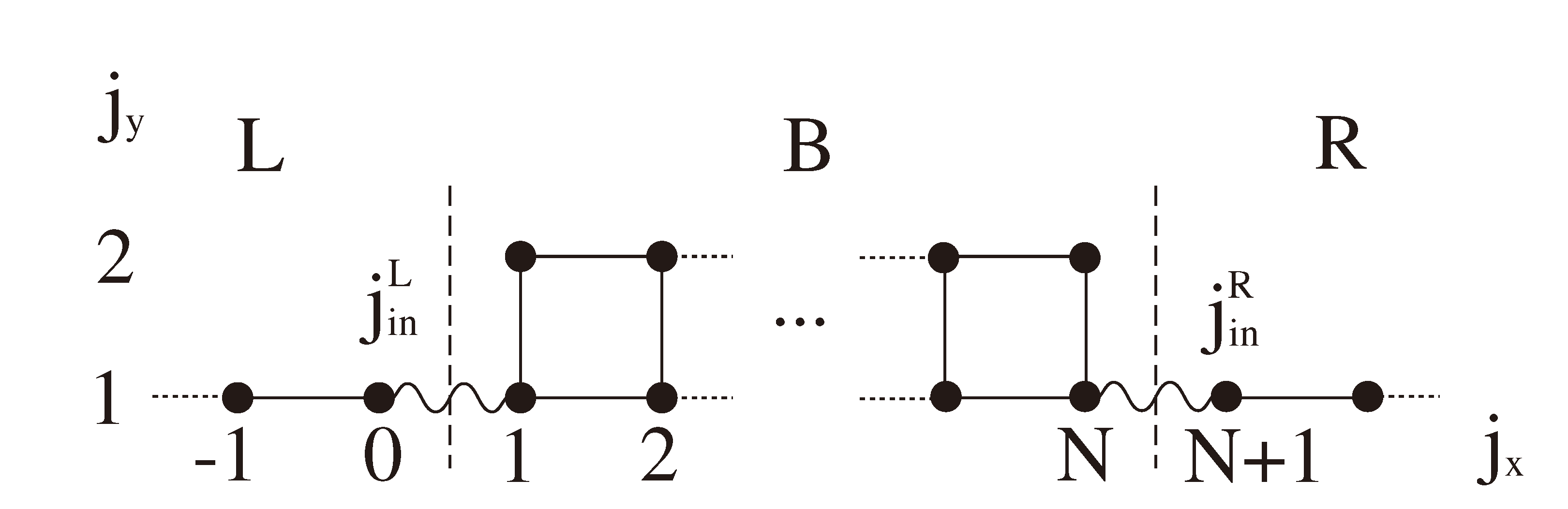
To visualize the idea of the tight-binding approach, Figure A1 displays the example of the 2D cavity connected to 1D electrodes. We can see that the matrix elements are nonzero only for at the connection to the right continuum and for at the connection to the left continuum. We introduce the coefficients
that are independent on energy. As a result, the matrix elements (A29) can be written in the form
where denotes the beginning of the semi-infinite electrode C. Taking into account the definition Equation (A33), the expression (A28) can be written in the form
Figure A1.
Connection between bounded system B and electrode C. The coupling operator is nonzero only for , and at the connection to the left electrode and for , and at the connection to the right electrode.
Figure A1.
Connection between bounded system B and electrode C. The coupling operator is nonzero only for , and at the connection to the left electrode and for , and at the connection to the right electrode.

In the tight-binding representation the electron wave function in the electrode C is (see Equation (A50))
where for the 1D tight-binding model the dispersion is used. The integration in Equation (A36) over zone from to yields [see Equation (A52)] the expression for matrix elements of the operator
The scattering matrix elements , describing the transition from a continuum to a continuum C at the incident energy E, are [37]
Inserting the resolution of identities , , by means of Equations (A19), (A23), (A30) and (A33), we obtain
Here, the function (see Figure A1) are the wave functions of the semi-infinite electrodes at the QPC.
Appendix A.1. Normalization Constant of the Electrode Eigenfunctions
We consider the electron eigenstate in the electrode as
with the normalization constant and . These functions must satisfy the equation
First, let us rewrite using dispersion relation at :
On the other hand, we have
The Lagrange’s trigonometric identity
helps us to write down
Taking into account the above results, we have for Equation (A44)
Comparing the left and the right sides of this equation, we obtain
Consequently, Equation (A41) becomes
Appendix A.2. Integral Over Zone
We recall that and
As a result, we have
Here we use the dispersion relation .
References
- Wolf, S.A. Spintronics: A Spin-Based Electronics Vision for the Future. Science 2001, 294, 1488–1495. [Google Scholar] [CrossRef] [PubMed] [Green Version]
- Žutić, I.; Fabian, J.; Sarma, D.S. Spintronics: Fundamentals and applications. Rev. Mod. Phys. 2004, 76, 323. [Google Scholar] [CrossRef] [Green Version]
- Hanson, R.; Kouwenhoven, L.P.; Petta, J.R.; Tarucha, S.; Vandersypen, L.M.K. Spins in few-electron quantum dots. Rev. Mod. Phys. 2007, 79, 1217–1265. [Google Scholar] [CrossRef] [Green Version]
- Engel, H.A.; Loss, D. Detection of Single Spin Decoherence in a Quantum Dot via Charge Currents. Phys. Rev. Lett. 2001, 86, 4648–4651. [Google Scholar] [CrossRef] [PubMed] [Green Version]
- Dehghan, E.; Khoshnoud, D.S.; Naeimi, A. Logical spin-filtering in a triangular network of quantum nanorings with a Rashba spin-orbit interaction. Phys. B Condens. Matter 2018, 529, 21–26. [Google Scholar] [CrossRef]
- Sattari, F.; Mirershadi, S. Spin-dependent transport properties in strained silicene with extrinsic Rashba spin-orbit interaction. J. Magn. Magn. Mater. 2018, 445, 6–10. [Google Scholar] [CrossRef]
- Pudlak, M.; Nazmitdinov, R.G. Spin-dependent electron transmission across the corrugated graphene. Physica E 2020, 118, 113846. [Google Scholar] [CrossRef] [Green Version]
- Lou, X.; Adelmann, C.; Crooker, S.A.; Garlid, E.S.; Zhang, J.; Reddy, K.S.M.; Flexner, S.D.; Palmstrm, C.J.; Crowell, P.A. Electrical detection of spin transport in lateral ferromagnet-semiconductor devices. Nat. Phys. 2007, 3, 197. [Google Scholar] [CrossRef] [Green Version]
- Dash, S.P.; Sharma, S.; Patel, R.S.; de Jong, M.P.; Jansen, R. Electrical creation of spin polarization in silicon at room temperature. Nature 2009, 462, 491. [Google Scholar] [CrossRef]
- Ciorga, M.; Einwanger, A.; Wurstbauer, U.; Schuh, D.; Wegscheider, W.; Weiss, D. Electrical spin injection and detection in lateral all-semiconductor devices. Phys. Rev. B 2009, 79, 165321. [Google Scholar] [CrossRef] [Green Version]
- Valín-Rodríguez, M.; Nazmitdinov, R.G. Model for spin-orbit effects in two-dimensional semiconductors in magnetic fields. Phys. Rev. B 2006, 73, 235306. [Google Scholar] [CrossRef] [Green Version]
- Fabian, J.; Matos-Abiague, A.; Ertler, C.; Stano, P.; Žutić, I. Semiconductor spintronics. Acta Phys. Slovaca 2007, 57, 565–907. [Google Scholar] [CrossRef] [Green Version]
- Nazmitdinov, R.G.; Pichugin, K.N.; Valín-Rodríguez, M. Spin control in semiconductor quantum wires: Rashba and Dresselhaus interaction. Phys. Rev. B 2009, 79, 193303. [Google Scholar] [CrossRef] [Green Version]
- Schliemann, J. Colloquium: Persistent spin textures in semiconductor nanostructures. Rev. Mod. Phys. 2017, 89, 011001. [Google Scholar] [CrossRef] [Green Version]
- Bychkov, Y.A.; Rashba, E.I. Oscillatory effects and the magnetic susceptibility of carriers in inversion layers. J. Phys. C Solid State Phys. 1984, 17, 6039–6045. [Google Scholar] [CrossRef]
- Rashba, E.I. Electron spin operation by electric fields: Spin dynamics and spin injection. Phys. Low-Dimens. Syst. Nanostruct. 2004, 20, 189–195. [Google Scholar] [CrossRef] [Green Version]
- Nitta, J.; Akazaki, T.; Takayanagi, H.; Enoki, T. Gate Control of Spin-Orbit Interaction in an Inverted In0.53Ga0.47As/In0.52Al0.48As Heterostructure. Phys. Rev. Lett. 1997, 78, 1335–1338. [Google Scholar] [CrossRef]
- Grundler, D. Large Rashba splitting in InAs quantum wells due to electron wave function penetration into the barrier layers. Phys. Rev. Lett. 2000, 84, 6074–6077. [Google Scholar] [CrossRef]
- Hu, C.M.; Nitta, J.; Akazaki, T.; Takayanagi, H.; Osaka, J.; Pfeffer, P.; Zawadzki, W. Zero-field spin splitting in an inverted In0.53Ga0.47As/In0.52Al0.48As heterostructure: Band nonparabolicity influence and the subband dependence. Phys. Rev. B 1999, 60, 7736–7739. [Google Scholar] [CrossRef]
- Lutchyn, R.M.; Sau, J.D.; Das Sarma, S. Majorana Fermions and a Topological Phase Transition in Semiconductor-Superconductor Heterostructures. Phys. Rev. Lett. 2010, 105, 077001. [Google Scholar] [CrossRef] [Green Version]
- Oreg, Y.; Refael, G.; von Oppen, F. Helical Liquids and Majorana Bound States in Quantum Wires. Phys. Rev. Lett. 2010, 105, 177002. [Google Scholar] [CrossRef] [PubMed] [Green Version]
- Mourik, V.; Zuo, K.; Frolov, S.M.; Plissard, S.R.; Bakkers, E.P.A.M.; Kouwenhoven, L.P. Signatures of Majorana Fermions in Hybrid Superconductor-Semiconductor Nanowire Devices. Science 2012, 336, 1003–1007. [Google Scholar] [CrossRef] [PubMed] [Green Version]
- Lucignano, P.; Mezzacapo, A.; Tafuri, F.; Tagliacozzo, A. Advantages of using high-temperature cuprate superconductor heterostructures in the search for Majorana fermions. Phys. Rev. B 2012, 86, 144513. [Google Scholar] [CrossRef] [Green Version]
- Klinovaja, J.; Loss, D. Time-reversal invariant parafermions in interacting Rashba nanowires. Phys. Rev. B 2014, 90, 045118. [Google Scholar] [CrossRef] [Green Version]
- Elliott, S.R.; Franz, M. Colloquium: Majorana fermions in nuclear, particle, and solid-state physics. Rev. Mod. Phys. 2015, 87, 137–163. [Google Scholar] [CrossRef] [Green Version]
- Sarma, S.D.; Freedman, M.; Nayak, C. Majorana zero modes and topological quantum computation. Quantum Inf. 2015, 1, 15001. [Google Scholar] [CrossRef] [Green Version]
- Aasen, D.; Hell, M.; Mishmash, R.V.; Higginbotham, A.; Danon, J.; Leijnse, M.; Jespersen, T.S.; Folk, J.A.; Marcus, C.M.; Flensberg, K.; et al. Milestones Toward Majorana-Based Quantum Computing. Phys. Rev. X 2016, 6, 031016. [Google Scholar] [CrossRef]
- Koga, T.; Nitta, J.; Akazaki, T.; Takayanagi, H. Rashba spin-orbit coupling probed by the weak antilocalization analysis in InAlAs/InGaAs/InAlAs quantum wells as a function of quantum well asymmetry. Phys. Rev. Lett. 2002, 89, 046801. [Google Scholar] [CrossRef]
- Governale, M.; Boese, D.; Zülicke, U.; Schroll, C. Filtering spin with tunnel-coupled electron wave guides. Phys. Rev. B 2002, 65, 140403. [Google Scholar] [CrossRef] [Green Version]
- Ohe, J.; Yamamoto, M.; Ohtsuki, T.; Nitta, J. Mesoscopic Stern-Gerlach spin filter by nonuniform spin-orbit interaction. Phys. Rev. B 2005, 72, 041308. [Google Scholar] [CrossRef] [Green Version]
- Wang, X.F.; Vasilopoulos, P. Spin-dependent transmission in waveguides with periodically modulated strength of the spin-orbit interaction. App. Phys. Lett. 2003, 83, 940–942. [Google Scholar] [CrossRef] [Green Version]
- Sakurai, J.J. Modern Quantum Mechanics; Addison-Wesley: Reading, MA, USA, 1994. [Google Scholar]
- Heiss, W.D.; Nazmitdinov, R.G. Orbital magnetism in small quantum dots with closed shells. J. Exp. Theor. Phys. Lett. 1998, 68, 915. [Google Scholar] [CrossRef] [Green Version]
- Könemann, J.; Haug, R.J.; Maude, D.K.; Fal’ko, V.I.; Altshuler, B.L. Spin-Orbit Coupling and Anisotropy of Spin Splitting in Quantum Dots. Phys. Rev. Lett. 2005, 94, 226404. [Google Scholar] [CrossRef] [PubMed] [Green Version]
- Valín-Rodríguez, M.; Puente, A.; Serra, L. Role of spin-orbit coupling in the far-infrared absorption of lateral semiconductor dots. Phys. Rev. B 2002, 66, 045317. [Google Scholar] [CrossRef] [Green Version]
- Mahaux, C.; Weidenmüller, H.A. Shell-Model Approach to Nuclear Reactions; North-Holland: Amsterdam, The Netherlands, 1969. [Google Scholar]
- Dittes, F.M. The decay of quantum systems with a small number of open channels. Phys. Rep. 2000, 339, 215–316. [Google Scholar] [CrossRef]
- Sadreev, A.F.; Rotter, I. S-matrix theory for transmission through billiards in tight-binding approach. J. Phys. A Math. Gen. 2003, 36, 11413–11433. [Google Scholar] [CrossRef] [Green Version]
- Kiselev, A.A.; Kim, K.W. Prohibition of equilibrium spin currents in multiterminal ballistic devices. Phys. Rev. B 2005, 71, 153315. [Google Scholar] [CrossRef] [Green Version]
- Zhai, F.; Xu, H.Q. Symmetry of Spin Transport in Two-Terminal Waveguides with a Spin-Orbital Interaction and Magnetic Field Modulations. Phys. Rev. Lett. 2005, 94, 246601. [Google Scholar] [CrossRef]
- Bulgakov, E.N.; Sadreev, A.F. Spin polarization in quantum dots by radiation field with circular polarization. J. Exp. Theor. Phys. Lett. 2001, 73, 505. [Google Scholar] [CrossRef]
- Ihn, T. Semiconductor Nanostructures: Quantum States and Electronic Transport; Oxford University Press: New York, NY, USA, 2010. [Google Scholar]
- Ando, T. Quantum point contacts in magnetic fields. Phys. Rev. B 1991, 44, 8017–8027. [Google Scholar] [CrossRef]
- Nazmitdinov, R.G.; Pichugin, K.N.; Rotter, I.; Šeba, P. Whispering gallery modes in open quantum billiards. Phys. Rev. E 2001, 64, 056214. [Google Scholar] [CrossRef] [PubMed] [Green Version]
- Nazmitdinov, R.G.; Pichugin, K.N.; Rotter, I.; Šeba, P. Conductance of open quantum billiards and classical trajectories. Phys. Rev. B 2002, 66, 085322. [Google Scholar] [CrossRef] [Green Version]
- Sandalov, I.; Nazmitdinov, R.G. Shell effects in nonlinear magnetotransport through small quantum dots. Phys. Rev. B 2007, 75, 075315. [Google Scholar] [CrossRef]
Figure 1.
Sketch of the 2D device that consists of a circular lateral QD. The effective QD’s confinement includes a constant potential with the Rashba interaction (gray region). Additional thin (0.1d) constant potential shell (dark gray region) controls the coupling between the QD and two electrodes.

Figure 2.
The probability for the direct transmission as function of the electron energy and the parameter . Red crosses indicate that correspond to = 0 for: , , .
Figure 2.
The probability for the direct transmission as function of the electron energy and the parameter . Red crosses indicate that correspond to = 0 for: , , .
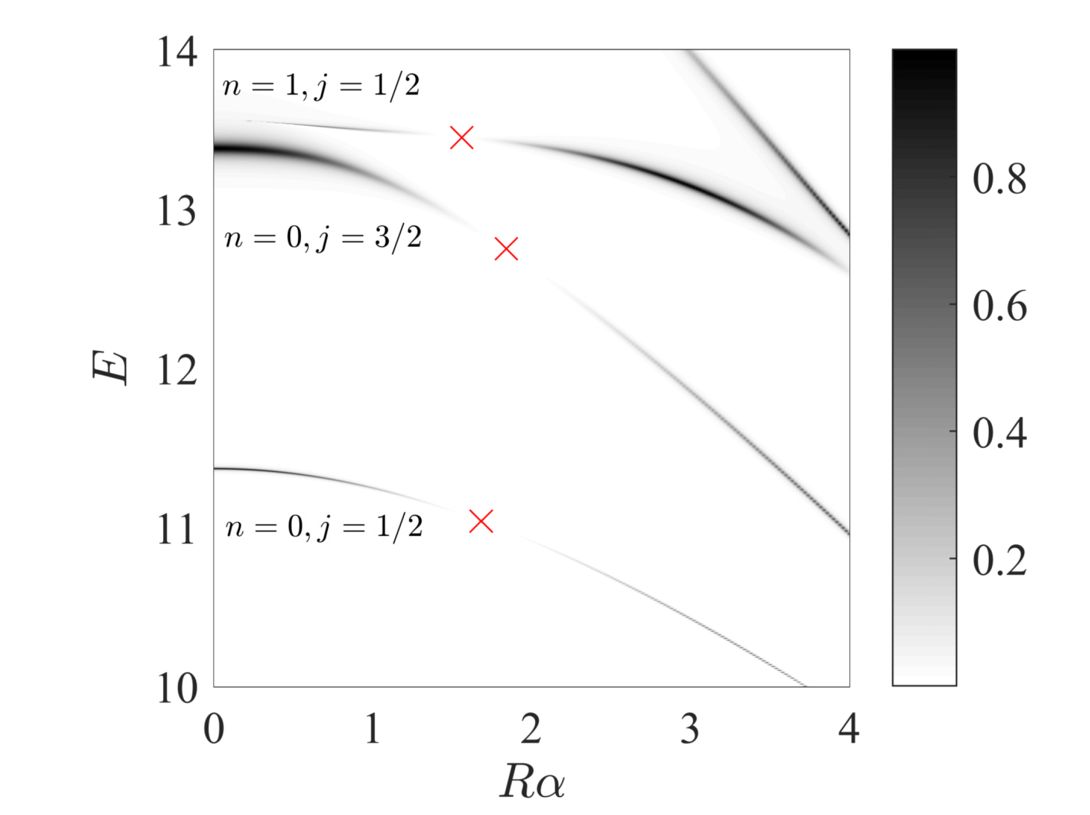
Figure 3.
Quantum dot with radius without any additional potential. The probability for the direct transmission as function of the electron energy and the parameter (a). Average effectivity of spin invertor over energy range (b).
Figure 3.
Quantum dot with radius without any additional potential. The probability for the direct transmission as function of the electron energy and the parameter (a). Average effectivity of spin invertor over energy range (b).


Table 1.
Value of for quantum numbers n and j.
| n | j | |
|---|---|---|
| 0 | 1/2 | 1.68 |
| 0 | 3/2 | 1.85 |
| 1 | 1/2 | 1.57 |
| 0 | 5/2 | 1.98 |
| 1 | 3/2 | 1.61 |
| 2 | 1/2 | 1.59 |
| 0 | 7/2 | 2.1 |
Publisher’s Note: MDPI stays neutral with regard to jurisdictional claims in published maps and institutional affiliations. |
© 2020 by the authors. Licensee MDPI, Basel, Switzerland. This article is an open access article distributed under the terms and conditions of the Creative Commons Attribution (CC BY) license (http://creativecommons.org/licenses/by/4.0/).
Share and Cite
MDPI and ACS Style
Pichugin, K.; Puente, A.; Nazmitdinov, R. Kramers Degeneracy and Spin Inversion in a Lateral Quantum Dot. Symmetry 2020, 12, 2043. https://doi.org/10.3390/sym12122043
AMA Style
Pichugin K, Puente A, Nazmitdinov R. Kramers Degeneracy and Spin Inversion in a Lateral Quantum Dot. Symmetry. 2020; 12(12):2043. https://doi.org/10.3390/sym12122043
Chicago/Turabian StylePichugin, Konstantin, Antonio Puente, and Rashid Nazmitdinov. 2020. "Kramers Degeneracy and Spin Inversion in a Lateral Quantum Dot" Symmetry 12, no. 12: 2043. https://doi.org/10.3390/sym12122043
Note that from the first issue of 2016, this journal uses article numbers instead of page numbers. See further details here.