Dynamic Behaviors Analysis of Asymmetric Stochastic Delay Differential Equations with Noise and Application to Weak Signal Detection

Department of Mathematical and Physics, Shijiazhuang Tiedao University, Shijiazhuang 050043, China
*
Author to whom correspondence should be addressed.
Symmetry 2019, 11(11), 1428; https://doi.org/10.3390/sym11111428
Submission received: 24 October 2019
/
Revised: 11 November 2019
/
Accepted: 15 November 2019
/
Published: 19 November 2019
Abstract
:This paper presents the dynamic behaviors of a second-order asymmetric stochastic delay system with a Duffing oscillator as well as through the detection of weak signals, which are analyzed theoretically and numerically. The dynamic behaviors of the asymmetric system are analyzed based on the stochastic center manifold, together with Hopf bifurcation. Numerical analysis revealed that the time delay could enhance the noise immunity of the asymmetric system so as to enhance the asymmetric system’s ability to detect weak signals. The frequency of the weak signal under noise excitation was detected through the ‘act-and-wait’ method. The small amplitude was detected through the transition from the chaotic to the periodic state. Theoretical analysis and numerical simulation indicate that the application of the asymmetric Duffing oscillator with delay to detect weak signal is feasible.
1. Introduction
The detection of weak signals is widely used in aerospace, engineering, transportation, as well as in biological, military, and other practical applications. For example, for high-speed motor vehicles, in order to ensure the safe use of key components bearings and wheels of a high-speed moving group, it is necessary to detect effective weak signals through condition monitoring [1] in a timely manner before the damage and failure of moving parts.
As for weak signal detection, fault diagnosis, and feature extraction, scholars have focused on two aspects in recent years, based on the transition from the chaotic state to the large-scale periodic state to detect a weak effective signal submerged in noise [2,3,4,5]. Using the stochastic resonance method and its transition characteristics makes a weak signal submerged in it stand out by using noise in the form of large scale transitions to identify the weak signal [6,7,8,9,10,11,12]. The method of stochastic resonance can not identify all kinds of weak signals processed by the stochastic resonance system, but rather only one kind of single-cycle that has the symmetrical characteristics of the weak signal. The chaotic oscillator can detect weak signals effectively because of its properties of noise immunity and sensitivity to specific frequency signals [2,13,14]. Therefore, the weak effective signal submerged in noise is detected by the transition from a chaotic state to a large-scale periodic state in this paper.
The nonlinear dynamic asymmetric systems used to detect weak signals are mainly as follows: Shi et al. [4] used the Holmes Duffing oscillator to work as the detection system. Zhao et al. [2] used the van der Pol-–Duffing oscillator to a detect weak signal. Wang and Gao used [5] the Novel butterfly-shaped model as the detection model. Zhang et al. [15] considered the Langevin system, which is composed of two single bistable systems by means of linear coupling driven by a Lévy noise and weak periodic signal to detect weak signals. Since the asymmetric Duffing equation is widely studied model in nonlinear asymmetric systems, which is sensitive to a weak signal of the specific frequency, we also use the asymmetric Duffing system to detect the effective weak signal submerged in noise.
At present, some scholars have studied the dynamic behaviors of asymmetric non-delay systems in detail [16,17,18]. In addition, time delay is universal in nature. The dynamic analysis of the asymmetric delay differential system has attracted more and more scholarly attention [19,20,21,22]. However there is less research for asymmetric stochastic delay systems. In [23], the author studied the stability of the asymmetric time-delayed linear control system under Gaussian white noise excitation. In [24], the study of time delay effects on the control of asymmetric linear systems under stochastic excitation has been presented. Guo et al. [25] analyzed bifurcations in an asymmetric stochastic time-delayed fractional biorhythmic biological system. In [26], the authors calculated the threshold of pitchfork and Hopf bifurcation in a stochastic delay differential equation and found that analyzing bifurcation thresholds in numerical simulations is very important. With respect to the asymmetric stochastic delay differential systems, the description of natural laws is more realistic, so it is of great significance to study the asymmetric stochastic delay differential systems.
Motivated by the above scholars’ research results and the actual engineering situation, this paper mainly aims to gain insight into the dynamic behaviors of a second-order asymmetric stochastic delay system with a Duffing oscillator and application to weak signal detection. The choice of an asymmetric delay differential system is not only rich in dynamic behavior, but also more realistic than the asymmetric ordinary differential equation. The reason for choosing Gaussian white noise is that Gaussian white noise can be regarded as the form derivative of the Wiener process and the power spectrum density in the whole frequency (,+∞) domain is constant and easy to calculate, thus its research has been very mature. The existence of weak effective signals and feature extraction of various information should follow the following order: Frequency → amplitude.
This paper is organized as follows: In Section 2, M.S. Fofana’s method is used to reduce the asymmetric delay differential equation to the asymmetric ordinary differential equation and the stochastic equation is derived theoretically [27]. Then the stochastic bifurcation condition of the asymmetric system is obtained. In Section 3, we use the method of the stochastic Melnikov function to derive the theoretical chaotic threshold. The results showed that the time delay feedback could enhance the detection ability of the asymmetric system to some extent. In Section 4, the feasibility of using the asymmetric stochastic delay system with the Duffing oscillator to detect a weak signal is verified by numerical simulation results.
2. Theoretical Analysis
We consider the second-order asymmetric stochastic delay system with a Duffing oscillator, subject to the weakly external excitation of Gaussian white noise.
The asymmetric system (1) can be organized:
where , , , , is the time delay, A is the feedback gain factor, is the damping item, is the built-in driving force, is the Gaussian white noise of intensity , and power spectral density K. The asymmetric system (1) has two saddle points and a center point (0, 0).
2.1. Stability Analysis
In this section, we calculate the transversality condition and analyze the stability of the linearized system of the asymmetric Duffing system (2), which is given by:
Its adjoint equation is:
Make , ) and , so the adjoint equation with respect to the bilinear pairing is:
which has eigenvalues satisfying asymmetric system (2)’s transcendental characteristic equation at the equilibrium point (0, 0):
Obviously, the asymmetric system does not have a zero characteristic root. From Equation (6), when the time delay we can obtain:
Its characteristic roots are =, if and only if > 0, then , thus the asymmetric system is asymptomatic stability at the equilibrium point (0, 0).
Theorem 1
Proof.
Setting the time delay are a pair of pure imaginary roots of Equation (6). We can obtain:
When the two equations above are squared and then added together, we can get the equation with respect to as follows:
Thus, we can figure out:
So when , are a pair of pure imaginary roots of Equation (6). Differentiating both sides of Equation (6) with respect to , yields:
Thus, we figure out:
Since the symbols of and are the same, if and only if:
then . Combined with the Hopf bifurcation theorem, the asymmetric system (2) will occur the Hopf bifurcation at (0, 0) and generate a limit cycle. □
2.2. Stochastic Equation
In this section, we use the mathematical idea [27,28] of reducing the asymmetric stochastic delay differential equation into an asymmetric ordinary differential equation to analyze the stochastic stability of the asymmetric system. At first, we carry out the stochastic center manifold of Equation (3) by studying the following approximate expression of .
Since the characteristic roots of the adjoint equation and the characteristic equation of the linear asymmetric system are the same, when . Project it onto the two disjoint subspaces and get the direct sum , then the base functions of Equations (3) and (4) under are as follows:
where the inner product matrix , has the following expression:
Substituting into the bilinear pairing expression (5) to get the nonsingular matrix as follows:
The basis of the adjoint equation is normalized to , a new base function expression is obtained:
Substituting generated by the new inner product matrix into Equation (12) and the available identity matrix is as follows:
Since and , we can easily obtain . With a definition , where . We have,
Similarly, holds. is the solution operator of the linearized equation. Thus, we obtain as the solution operator of the adjoint equation in C.
Theorem 2.
Set , , is the unique solution of Equation (1), where , , and are in P, Q, respectively. Under the semigroup and its infinitesimal generator , the projected solutions , and onto P, Q respectively are invariant. Then under the change of variables , a first-order approximation for is as follows:
The following asymmetric stochastic center manifold form can be obtained from the analysis of Theorems 1 and 2.
Theorem 3.
If the conditions of Theorems 1 and 2 are satisfied, the asymmetric stochastic center manifold of Equation (1) is as follows:
Making a change of variables, namely
Setting , the available inverse transformation yield the following:
and then we can obtain the asymmetric center manifold as follows:
where,
The asymmetric system can be modeled into It asymmetric stochastic differential equations as follows:
where is a standard Wiener process.
The Hamiltonian corresponding to Equation (14) is as follows:
where .
Therefore, the asymmetric system in Equation (14) can be written as a asymmetric stochastic Hamiltonian system as follows:
where,
According to the well-known stochastic averaging method, the It stochastic averaging Hamiltonian is obtained.
Theorem 4
In the following, based on the above analysis, the local stability of the asymmetric stochastic delay Duffing system is studied.
Theorem 5.
Set as the real number defined by Equation (15), if and only if , then the trivial solution of the asymmetric stochastic delay Duffing system is the local asymptomatic stabilization with a probability density of 1.
Proof.
According to Theorem 4, we can obtain the linear equation corresponding to :
According to the Lyapunov exponent definition, the approximate value of the Lyapunov exponent is available:
Let , then the trivial solution of the asymmetric stochastic delay Duffing system is a local asymptomatic stabilization with a probability density of 1. □
Next, the qualitative state of the one-dimensional diffusion process is studied, which mainly depends on the characteristics of the drifting coefficient and the diffusion coefficient on the two boundaries.
Theorem 6.
Set as the real numbers defined by Equation (15), if and only if . The trivial solution of the asymmetric stochastic delay Duffing system is global instability with a probability density of 1.
Proof.
According to the singular boundary theory, the left boundary is the first kind of singular boundary. Its diffusion coefficient , drifting coefficient , and characteristic value . If , the boundary is the regular boundary and if , the is the entrance boundary.
The right boundary is the second kind of singular boundary. When , the boundary is out of the boundary. When , the is the entrance boundary. Thus when , the trivial solution of the asymmetric stochastic delay Duffing system is global instability with a probability density of 1. □
Theorem 7.
Set as the real numbers defined by Equation (15), if and only if , D-bifurcation occurs and P-bifurcation occurs .
Proof.
When , then , the is the entrance boundary, the systematic state depends only on the left boundary.
According to the three-exponent method, the left boundary is the first kind of singular boundary, then we obtain representation as follows:
The equation can be simplified to:
and thus infer that the D-bifurcation occurs at and the P-bifurcation occurs at . □
3. Weak Signal Detection
Some of the failures that may occur in the engineering can often cause significant losses, so detecting weak signals can reduce or avoid system failures. The asymmetric chaos system is very sensitive to weak signals with similar external excitation, so it can detect weak signals very well.
3.1. Chaos in the Asymmetric Stochastic Delay Differential Equation
In this section, the necessary conditions for chaos in the asymmetric system (1) are derived by using the Melnikov method under the mean-square criterion.
The Hamiltonian in the linear part of the asymmetric Duffing system is:
Two different heteroclinic orbits are available:
Melnikov’s function for the heteroclinic orbit is:
where,
represents the stochastic part of the Melnikov process caused by noise, since is a smooth stochastic process. Therefore , the first moment of is:
The second moment of is:
where is the power spectral density of the Gaussian noise and is the frequency response function of the system obtained through Fourier transform:
Substituting into the above formula, we can obtain:
According to the residual theorem, we can obtain:
The power spectral density function of Gaussian white noise is , and the second moment of :
The asymmetric system’s stochastic Melnikov function appears a simple zero if and only if under the mean-square criterion. Subjected on the constraint of energy conservation and we have:
Based on the Melnikov process, the criterion for the possible chaotic motion is given:
If the parameter f is satisfied:
the asymmetric system may appear to be chaotic under the meaning of Smale.
Therefore, the threshold of the asymmetric system (1) is:
3.2. Time-Delayed Feedback and System Detection Capability
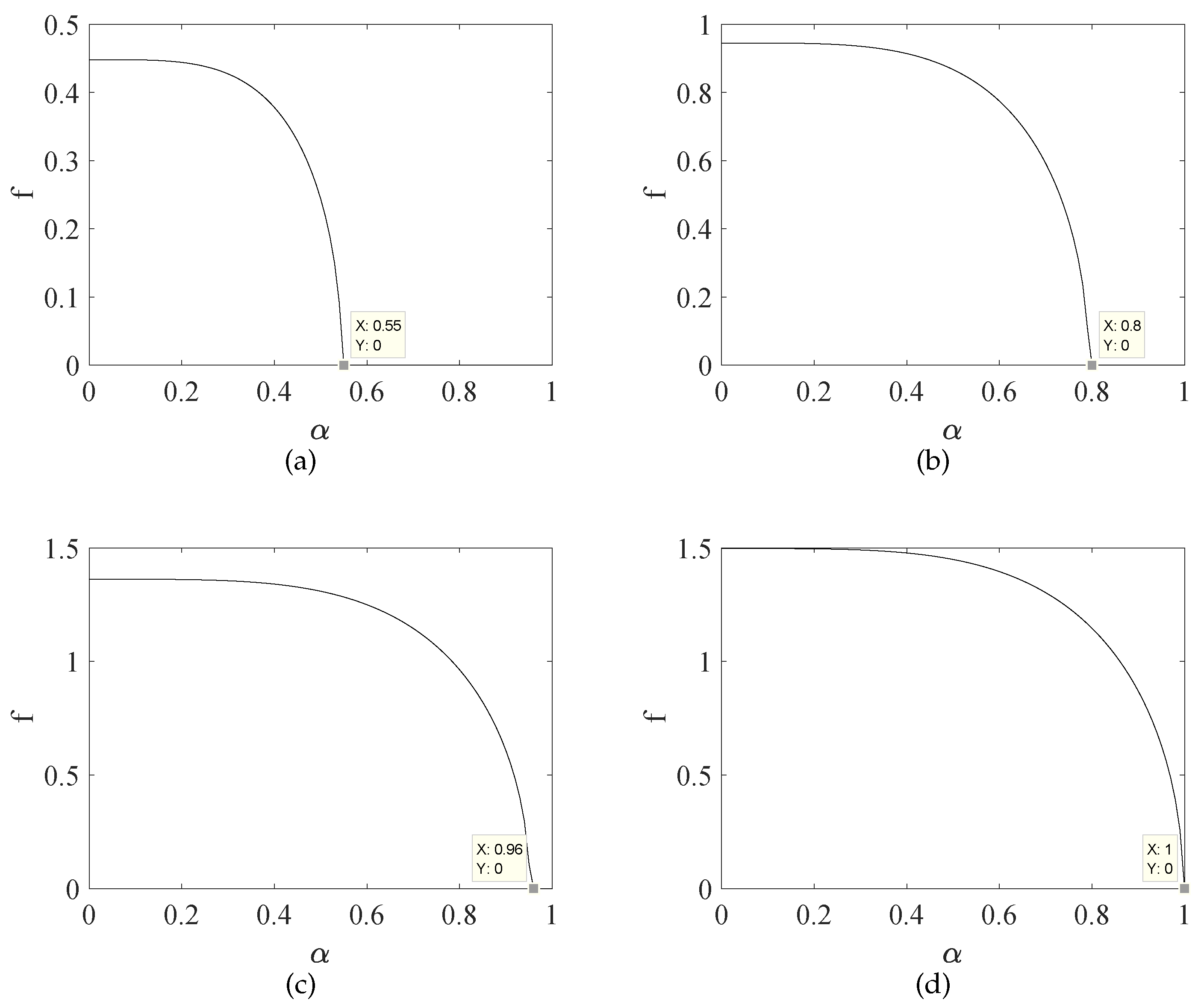
The following consideration is given to the change of the threshold with Gaussian white noise intensity under the influence of time delay. First fix parameters: , , , and according to the asymmetric system (1), increasing the time delay from to 3. Set the range of changes in Gaussian white noise intensity . According to [28], the power spectral density of Gaussian white noise is . The threshold of the asymmetric system (1) varies with the noise intensity under time-delayed feedback as shown in Figure 1.
The chaotic oscillator is highly effective in weak signal detection because of its properties of noise immunity and sensitivity to a specific frequency signal [2,13,14]. However this noise immunity is limited. When there is noise with a higher intensity, chaos is caused by the noise rather than being immune to the noise. This is reflected in Figure 1. We can see that when the noise intensity exceeds a certain value, no obvious chaos threshold can be found, which eliminates our hope of detecting signals by using state transition. From Figure 1a–d, the increase of time delay drags the curve to the right. The time-delay feedback control also obtains an effective threshold for the noise with a higher intensity. In other words, the asymmetric system response information is constantly added into the system through the time-delay feedback control, which makes the chaos caused by noise excitation delayed. The analytical results show that time-delay can effectively enhance the detection ability of the asymmetric system.
4. Numerical Simulation
Based on the actual engineering situation, we do not know whether the weak signal exists or not, so its frequency is generally unknown. However, when detecting the amplitude of the asymmetric stochastic delay system by state transition, we need to predict the frequency of the weak signal. Therefore, for the detection of weak signal, we should first determine the frequency information and then extract the amplitude information. Add a weak signal to the asymmetric system (1) to yield the following asymmetric system:
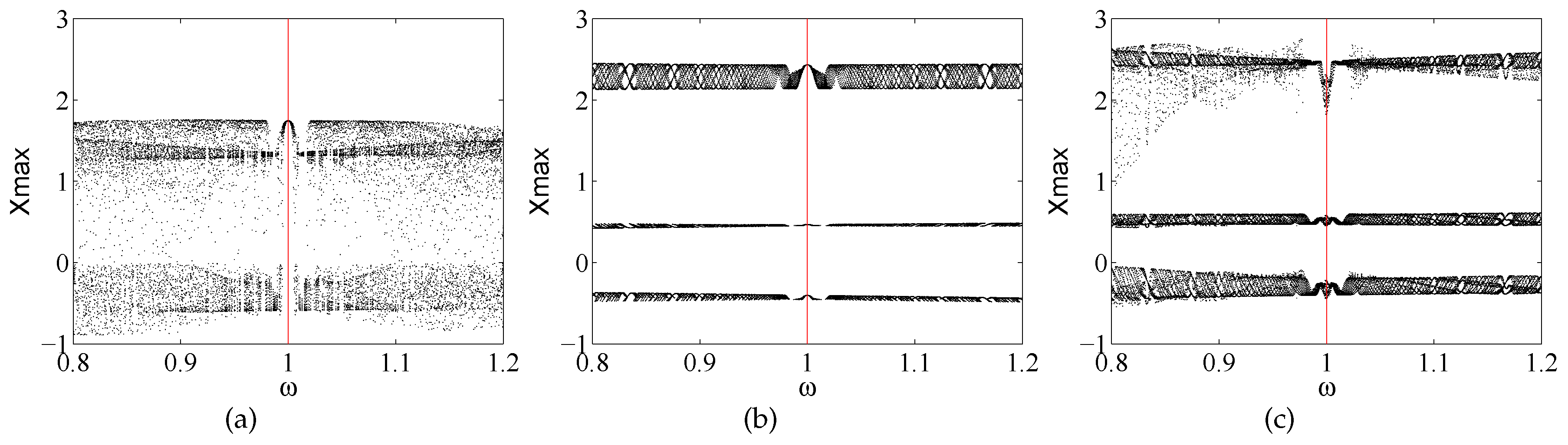
First fix parameters: , , , , , , and The amplitude of the weak signal is fixed at , , and respectively. The bifurcation diagrams of the frequency at which the asymmetric system identifies the weak signal are shown in Figure 2.
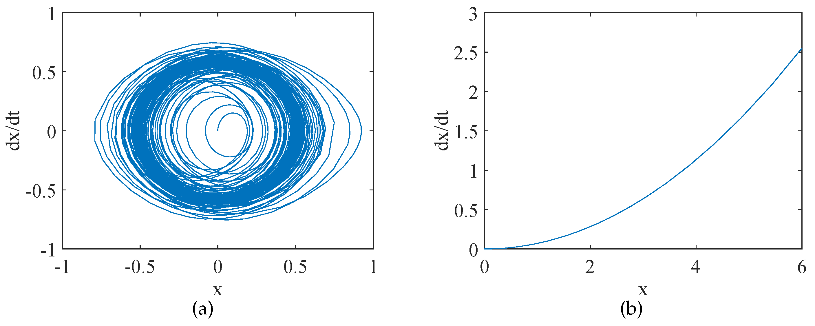
When , the phase diagrams when and are respectively drawn are shown in Figure 3.
As shown in Figure 2 and Figure 3, after adding the weak signal to the asymmetric system, fix the amplitude of the external excitation at and change . When , the asymmetric system is in a chaotic state. When , the chaotic state of the asymmetric system have the ‘act-and-wait’ [29] action. When , the asymmetric system is in a chaotic state again. The asymmetric system have an ‘act-and-wait’ action that detects the presence and frequency of the weak signal. With different values of amplitude r, we can find that the chaotic state always has the ‘act-and-wait’ action, thus we can extract the frequency of the weak signal under the unknown amplitude r. We propose for the first time to detect the frequency of weak effective signal by using the ‘act-and-wait’ action in the chaotic state.
Then the amplitude of the weak effective signal in noise is detected by the transition for the asymmetric system from chaos to large-scale periodicity. First fix parameters: , , , , and . Substituting into Equation (16) and we can get that the theoretical threshold is . The bifurcation diagram of asymmetric system (1) is shown in Figure 4.
As shown in Figure 4, the transition from chaos to periodicity of the motion of the asymmetric system (1) occurs at a certain threshold, and the phase diagrams of the asymmetric system (1), when , and , respectively, correspond to the phase diagrams as shown in the Figure 5.
When , there is the first transition of the asymmetric system from chaos to the periodicity and when , there is a second transition of the asymmetric system from periodicity to chaos. In this paper, the critical value of the first transition is the threshold of the asymmetric system . Then we can determine that the chaos threshold is . Therefore, the relative error between the numerical solution of the asymmetric system and the theoretical solution is:
Because the asymmetric chaos system (17) is very sensitive to small weak signal with similar excitation frequencies outside the asymmetric system, Melnikov method is still used to calculate the chaos threshold under the mean-square criterion of the asymmetric system which under the combined excitation of Gaussian white noise, time delay and weak signal, thus the amplitude calculation formula of the weak signal can be inferred and the weak signal can be identified.
The asymmetric system (17)’s chaos threshold is:
The formula for calculating the weak signal amplitude value is:
Fix the parameter: , , , , , and . Substituting into Equation (18) and we can get that the theoretical threshold is . The bifurcation diagram of the asymmetric system (17) is shown in Figure 6.
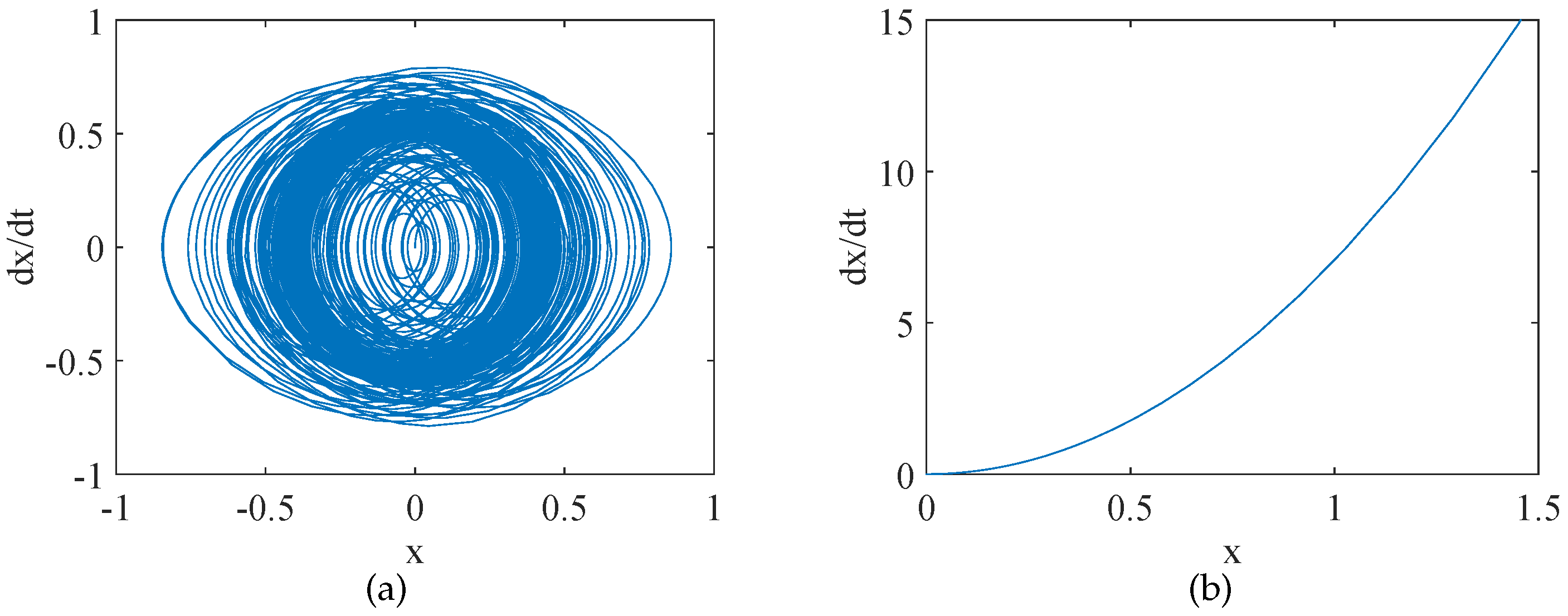
As shown in Figure 6, there is a transition of the asymmetric system (17) from chaos to the periodicity. The phase diagrams of the asymmetric system (17) are shown in the Figure 7.
The numerical solution for the transition of the asymmetric system (17) from chaos to periodicity can be determined as . The theoretical value of the asymmetric system (17) is , so the relative error between the numerical solution and the theoretical solution of the asymmetric system (17) is:
It is seen from the relative errors that the theoretical analytical results agree quite well with those from numerical simulation. According to Equation (19), the amplitude of the weak signal of the asymmetric system (17) can be calculated as . Thus numerical simulation indicate the feasibility of using the asymmetric stochastic delay system with a Duffing oscillator to detect weak signal.
The signal-to-noise ratio threshold of the asymmetric system is:
The signal-to-noise ratio of the second-order asymmetric stochastic delay system with a Duffing oscillator is −43 dB. The asymmetric system has a lower signal-to-noise ratio indicating that the asymmetric system has advantages in weak signal detection.
5. Conclusions
In this paper, firstly, the dynamic behavior of the second-order asymmetric stochastic delay system with a Duffing oscillator were analyzed. Based on the center manifold theorem, asymmetric stochastic averaging equation, and Lyapunov exponent, the stable and unstable conditions of the second-order asymmetric stochastic delay system with a Duffing oscillator were calculated. Secondly, the frequency of weak effective signal in noise was detected by the chaotic state having the ‘act-and-wait’ action. The amplitude of weak effective signal in noise was detected by the transition for the asymmetric system from the chaos to the large-scale periodicity. By theoretical analysis and numerical simulation, we found that the dynamic behaviors of the asymmetric system were affected by Gaussian white noise and time delay, and the time delay could be used to enhance the asymmetric system’s ability to detect weak signals. Thirdly, this paper mainly used the asymmetric stochastic delay Duffing system to detect weak signals. At present, we have not found any scholars who have considered nonlinear asymmetric stochastic delay systems to detect weak signals.
In this paper, only Gaussian white noise was considered, but non-Gaussian noise such as colored noise was not considered. In addition, the additive noise was considered in this paper instead of the more complex multiplicative noise. For frequency detection method, the stochastic resonance method could be considered [30,31].
Author Contributions
The authors contributed equally in writing this article. All authors read and approved the final manuscript.
Funding
This work was supported by the Natural Science Foundation of China [No. 11602151, 11872253]; Natural Science Foundation for Outstanding Young Researcher in Hebei Province of China [No. A2017210177]; Hundred Excellent Innovative Talents in Hebei Province [SLRC2019037]; The Key Project of Education Department in Hebei Province of China [No. ZD2016151]; Basic Research Team Special Support Projects [No. 311008]; and The Foundation of Hebei Education Department of China [Grant No. QN2018050].
Conflicts of Interest
The authors declare no conflict of interest.
References
- Martínez-García, M.; Zhang, Y.; Wan, J.; McGinty, J. Visually Interpretable Profile Extraction with an Autoencoder for Health Monitoring of Industrial Systems. In Proceedings of the International Conference on Advanced Robotics and Mechatronics, Toyonaka, Japan, 3–5 July 2019; pp. 649–654. [Google Scholar]
- Zhao, Z.H.; Yang, S.P. Application of van der Pol–Duffing oscillator in weak signal detection. Comput. Electr. Eng. 2015, 41, 1–8. [Google Scholar]
- Zheng, S.Y.; Guo, H.X.; Li, Y.A.; Wang, B.; Zhang, P. A new method for detecting line spectrum of ship-radiated noise using Duffing oscillator. Chin. Sci. Bull. 2007, 52, 1906–1912. [Google Scholar] [CrossRef]
- Shi, H.C.; Li, W.L. Research on Weak Resonance Signal Detection Method Based on Duffing Oscillator. Procedia Comput. Sci. 2017, 107, 460–465. [Google Scholar] [CrossRef]
- Wang, L.Z.; Gao, Y.F. Detection of weak signal in strong noise based on nbs chaos system. Procedia Eng. 2011, 23, 754–759. [Google Scholar] [CrossRef]
- He, B.; Huang, Y.; Wang, D.; Yan, B.; Dong, D. A parameter-adaptive stochastic resonance based on whale optimization algorithm for weak signal detection for rotating machinery. Measurement 2019, 136, 658–667. [Google Scholar] [CrossRef]
- Lu, S.; Zheng, P.; Liu, Y.; Cao, Z.; Yang, H.; Wang, Q. Sound-aided vibration weak signal enhancement for bearing fault detection by using adaptive stochastic resonance. J. Sound Vib. 2019, 449, 18–29. [Google Scholar] [CrossRef]
- Wang, Y.; Jiao, S.; Zhang, Q.; Lei, S.; Qiao, X. A weak signal detection method based on adaptive parameter-induced tri-stable stochastic resonance. Chin. J. Phys. 2018, 56, 1187–1198. [Google Scholar] [CrossRef]
- Li, Z.X.; Shi, B.Q. A piecewise nonlinear stochastic resonance method and its application to incipient fault diagnosis of machinery. Chin. J. Phys. 2019, 59, 126–137. [Google Scholar] [CrossRef]
- Wu, X.; Guo, W.; Cai, W.; Shao, X.; Pan, Z. A method based on stochastic resonance for the detection of weak analytical signal. Talanta 2003, 61, 863–869. [Google Scholar] [CrossRef]
- Kosko, B.; Mitaim, S. Stochastic resonance in noisy threshold neurons. Neural Netw. 2003, 16, 755–761. [Google Scholar] [CrossRef]
- Mitaim, S.; Kosko, B. Adaptive stochastic resonance. Proc. IEEE 1998, 86, 2152–2183. [Google Scholar] [CrossRef]
- Li, Y.; Yang, B. The chaotic detection of periodic short-impulse signals under strong noise background. J. Electron. 2002, 19, 431–433. [Google Scholar] [CrossRef]
- Wang, G.; Zheng, W.; He, S. Estimation of amplitude and phase of a weak signal by using the property of sensitive dependence on initial conditions of a nonlinear oscillator. Signal Process. 2002, 82, 103–115. [Google Scholar] [CrossRef]
- Zhang, G.; Hu, D.; Zhang, T. The analysis of stochastic resonance and bearing fault detection based on linear coupled bistable system under lévy noise. Chin. J. Phys. 2018, 56, 2718–2730. [Google Scholar] [CrossRef]
- Guo, X.; Zhang, G.; Tian, R. Periodic Solution of a Non-Smooth Double Pendulum with Unilateral Rigid Constrain. Symmetry 2019, 11, 886. [Google Scholar] [CrossRef]
- Wang, G.; Xiao, R.; Xu, C.; Huang, R.; Hao, X. Stability analysis of integrated power system with pulse load. Int. J. Electr. Power Energy Syst. 2020, 115, 105462. [Google Scholar] [CrossRef]
- Schwaller, B.; Ensminger, D.; Dresp-Langley, B.; Ragot, J. State estimation for a class of nonlinear systems. Int. J. Appl. Math. Comput. Sci. 2013, 23, 383–394. [Google Scholar] [CrossRef]
- Wang, Q. Bifurcation analysis in a predator–prey model for the effect of delay in prey. Int. J. Biomath. 2016, 9, 1650061. [Google Scholar] [CrossRef]
- Liu, M.Z.; Wang, Q. Numerical Hopf bifurcation of linear multistep methods for a class of delay differential equations. Appl. Math. Comput. 2009, 208, 462–474. [Google Scholar] [CrossRef]
- Wang, Q.; Li, D.; Liu, M.Z. Numerical Hopf bifurcation of Runge–Kutta methods for a class of delay differential equations. Chaos Solitons Fractals 2009, 42, 3087–3099. [Google Scholar] [CrossRef]
- Martínez-García, M.; Zhang, Y.; Gordon, T. Memory Pattern Identification for Feedback Tracking Control in Human–Machine Systems. Hum. Factors 2019. [Google Scholar] [CrossRef] [PubMed]
- Grigoriu, M. Control of time delay linear systems with Gaussian white noise. Probabilistic Eng. Mech. 1997, 12, 89–96. [Google Scholar] [CrossRef]
- Di Paola, M.; Pirrotta, A. Time delay induced effects on control of linear systems under random excitation. Probabilistic Eng. Mech. 2001, 16, 43–51. [Google Scholar] [CrossRef]
- Guo, Q.; Sun, Z.K.; Xu, W. Bifurcations in a fractional birhythmic biological system with time delay. Commun. Nonlinear Sci. Numer. Simul. 2019, 72, 318–328. [Google Scholar] [CrossRef]
- Lepine, F.; Vinals, J. Pitchfork and Hopf bifurcation threshold in stochastic equations with delayed feedback. arXiv 2008, arXiv:0810.4348. [Google Scholar]
- Fofana, M.S. Asymptotic stability of a stochastic delay equation. Probabilistic Eng. Mech. 2002, 17, 385–392. [Google Scholar] [CrossRef]
- Zhu, W.Q.; Cai, G.Q. Introduction to Stochastic Dynamics; Science Press: Beijing, China, 2017; p. 72. [Google Scholar]
- Martinez-Garcia, M.; Zhang, Y.; Gordon, T. Modeling lane keeping by a hybrid open-closed-loop pulse control scheme. IEEE Trans. Ind. Inform. 2016, 12, 2256–2265. [Google Scholar] [CrossRef]
- Wang, S.; Wang, F.; Wang, S.; Li, G. Detection of multi-frequency weak signals with adaptive stochastic resonance system. Chin. J. Phys. 2018, 56, 994–1000. [Google Scholar] [CrossRef]
- Guo, W.; Zhou, Z.; Chen, C.; Li, X. Multi-frequency weak signal detection based on multi-segment cascaded stochastic resonance for rolling bearings. Microelectron. Reliab. 2017, 75, 239–252. [Google Scholar] [CrossRef]
Figure 1.
The time delay enhances the noise immunity of chaotic state: (a) ; (b) ; (c) ; (d) .

Figure 2.
Bifurcation diagrams of the asymmetric system (1) with respect to frequency : (a) ; (b) ; and (c) .
Figure 2.
Bifurcation diagrams of the asymmetric system (1) with respect to frequency : (a) ; (b) ; and (c) .

Figure 3.
Phase diagrams of the asymmetric system (1): (a) and (b) .

Figure 4.
Bifurcation diagram of the asymmetric system (1).
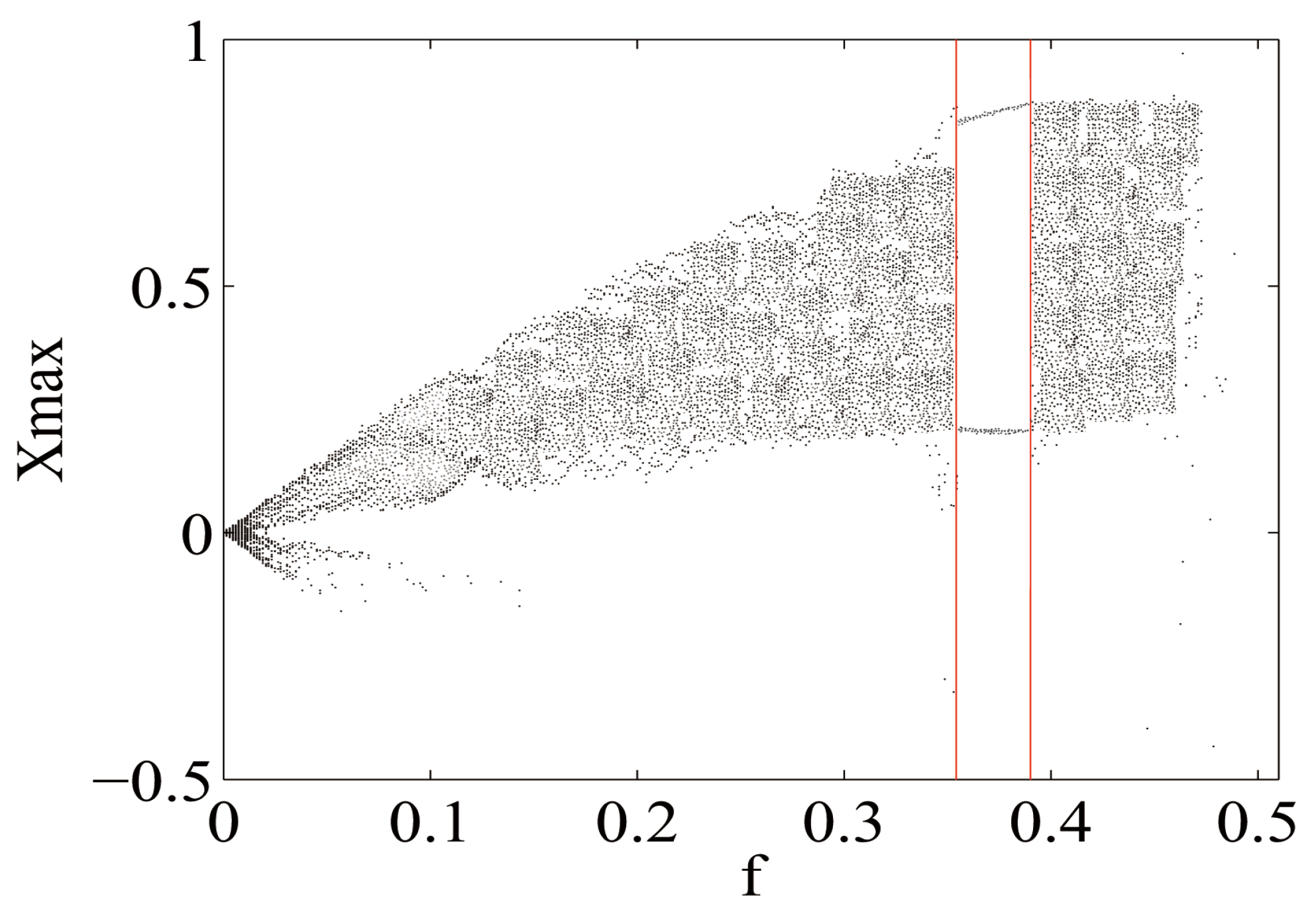
Figure 5.
Phase diagrams of the asymmetric system (1): (a) ; (b) ; and (c) .
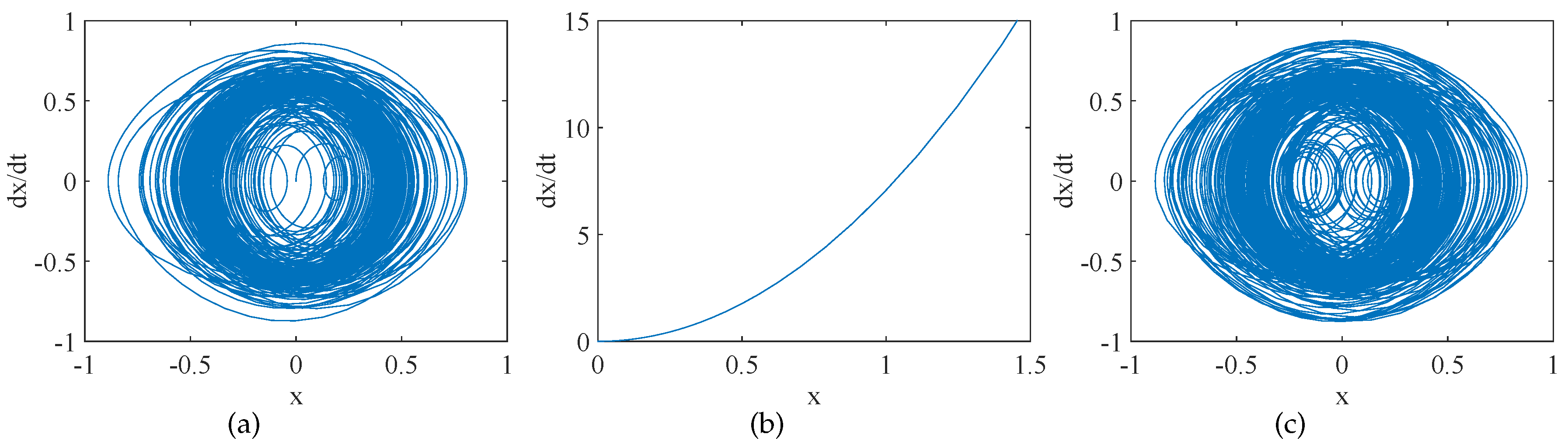
Figure 6.
Bifurcation diagram of the asymmetric system (17).
Figure 6.
Bifurcation diagram of the asymmetric system (17).
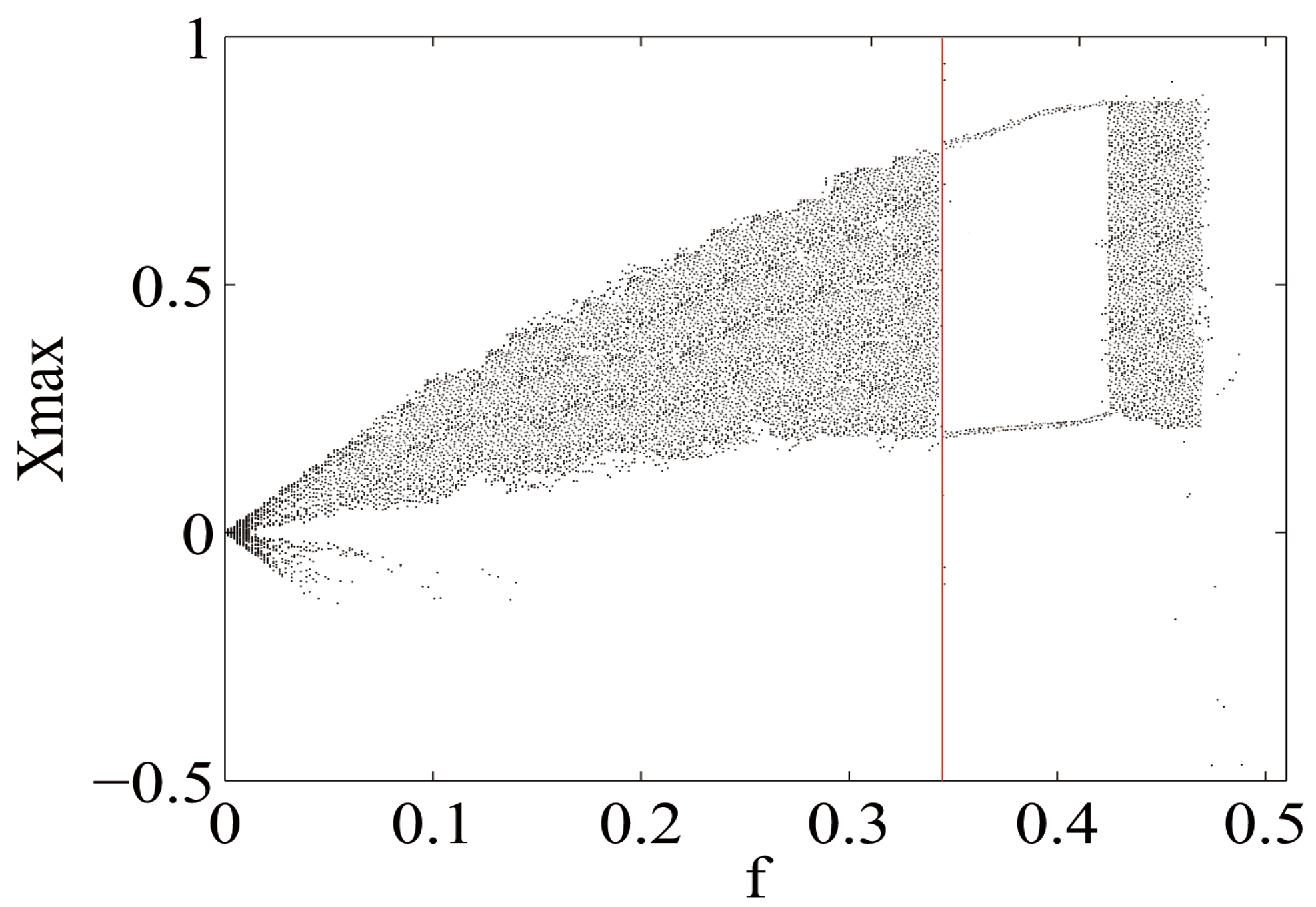
Figure 7.
Phase diagrams of the asymmetric system (17): (a) and (b) .
Figure 7.
Phase diagrams of the asymmetric system (17): (a) and (b) .
© 2019 by the authors. Licensee MDPI, Basel, Switzerland. This article is an open access article distributed under the terms and conditions of the Creative Commons Attribution (CC BY) license (http://creativecommons.org/licenses/by/4.0/).
Share and Cite
MDPI and ACS Style
Wang, Q.; Zhang, X.; Yang, Y. Dynamic Behaviors Analysis of Asymmetric Stochastic Delay Differential Equations with Noise and Application to Weak Signal Detection. Symmetry 2019, 11, 1428. https://doi.org/10.3390/sym11111428
AMA Style
Wang Q, Zhang X, Yang Y. Dynamic Behaviors Analysis of Asymmetric Stochastic Delay Differential Equations with Noise and Application to Weak Signal Detection. Symmetry. 2019; 11(11):1428. https://doi.org/10.3390/sym11111428
Chicago/Turabian StyleWang, Qiubao, Xing Zhang, and Yuejuan Yang. 2019. "Dynamic Behaviors Analysis of Asymmetric Stochastic Delay Differential Equations with Noise and Application to Weak Signal Detection" Symmetry 11, no. 11: 1428. https://doi.org/10.3390/sym11111428
Note that from the first issue of 2016, this journal uses article numbers instead of page numbers. See further details here.