Closed Form Solutions for Nonlinear Oscillators Under Discontinuous and Impulsive Periodic Excitations


Mechanical Engineering, Wayne State University, Detroit, MI 48202, USA
Symmetry 2019, 11(11), 1420; https://doi.org/10.3390/sym11111420
Submission received: 9 October 2019
/
Revised: 10 November 2019
/
Accepted: 12 November 2019
/
Published: 16 November 2019
(This article belongs to the Special Issue Asymptotic Methods in the Mechanics and Nonlinear Dynamics)
Abstract
:Periodic responses of linear and nonlinear systems under discontinuous and impulsive excitations are analyzed with non-smooth temporal transformations incorporating temporal symmetries of periodic processes. The related analytical manipulations are illustrated on a strongly nonlinear oscillator whose free vibrations admit an exact description in terms of elementary functions. As a result, closed form analytical solutions for the non-autonomous strongly nonlinear case are obtained. Conditions of existence for such solutions are represented as a family of period-amplitude curves. The family is represented by different couples of solutions associated with different numbers of vibration half cycles between any two consecutive pulses. Poincaré sections showed that the oscillator can respond quite chaotically when shifting from the period-amplitude curves.
1. Introductory Remarks and Example
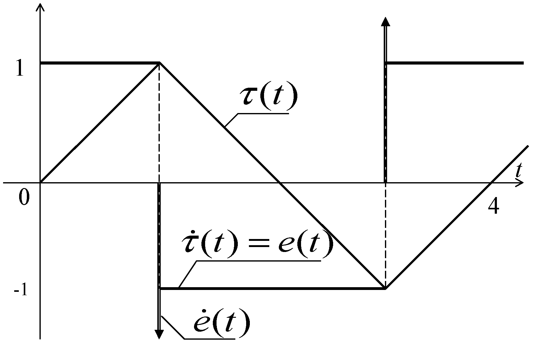
Impact loads applied to physical systems are often modeled with Dirac’s generalized functions (distributions) by ignoring the short-term load profiles and using their integral effects instead. However, the presence of distributions in a differential equation of motion requires the entire equation to be considered within the theory of distributions that leads to theoretical complications especially in nonlinear cases [1,2]. In the present work, we illustrate non-smooth temporal substitutions incorporating the pulse effects into a periodic time folding argument. Substituting such an argument into the differential equation of motion generates singularities of derivatives that can be effectively used to balance the loading Dirac’s delta impulses or discontinuities from the differential equations. In this introductory section, we outline necessary analytical manipulations based on general time symmetries of periodic processes regardless their temporal mode shapes. Namely, any periodic process admits time shifts with reflections. Such properties can be easily incorporated into the corresponding differential equations at the preliminary stage of study by means of the following standard pair of non-smooth periodic functions
As follows from the graphical illustration in Figure 1, the couple of functions and can be interpreted as a coordinate and velocity of a small particle oscillating between two perfectly stiff barriers without energy loss.
Note that the derivative remains undefined at discontinuity points . Also, since is a rectangular cosine-wave with step-wise discontinuities, its first generalized derivative is given by the periodic sequence of Dirac’s - functions as
Distribution (2) associates with the impulsive force applied from the barriers to the particle whenever the particle strikes the barriers. In addition, the following differential and algebraic properties hold
Although functions (1) are quite specific, they create a general basis for considering a broader class of oscillating processes. This is based on the statement that any periodic process of the period admits representation in the form of ‘hyperbolic number’ [3,4]
where , , and
Here, the terms and depict the sin- and cos-type symmetries, and can be viewed as “real” and “imaginary” parts of the hyperbolic number due to the relationship (3). Note that the term ‘hyperbolic number’ represents one of the multiple versions typically applied to the abstract algebraic combination [5], (). In our case, the unipotent is represented by the periodic step-wise discontinuous function describing the velocity of impact oscillator. Identity (4) can be easily proved by substituting (5) in (4) and considering the result on one period ; see Appendix A. The following example reveals temporal symmetries of the both components in (4)
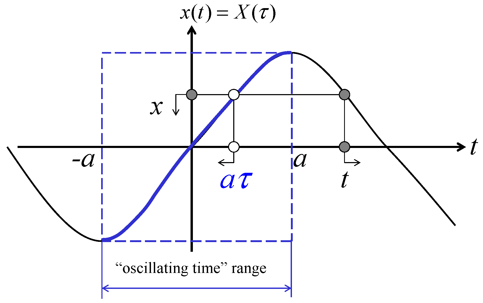
In particular, if a periodic function is even with respect to the quarter of period , then and identity (4) has only the “real component” . The corresponding geometrical interpretation is shown in Figure 2.
Let us outline some algebraic and differential properties of representation (4).
- Algebraic properties. Taking into account that , , ,…, gives, for instance,andGenerallywhereRelationship (6) is proved by setting and then solving the two equations for and .
- Differential properties. Despite of the presence of non-smooth and discontinuous functions on the right-hand side of identity (4), its class of smoothness coincides with a class of smoothness of the function . Namely, the behavior of the right-hand side of (4) in the neighborhoods of singularities is determined by the functions and . For instance, if then as or . However, if the function has inherent step-wise discontinuities at points then quantities will represent the steps of such discontinuities. Now assuming and taking the formal time derivative of (4) giveswhere is a generalized derivative with δ-type singularities at to be eliminated by imposing condition
Therefore, due to condition (8), derivative (7) still preserves the structure of hyperbolic number. If then the procedure (7)–(8) can be reiterated n times by sequentially imposing boundary conditions on the functions , and their derivatives at .
Further, we use the identity (4) as a representation for solutions of differential equations by considering and as a couple of new unknown functions of the temporal argument . In order to illustrate the corresponding manipulations, let us consider the equation
where the input function is periodic step-wise discontinuous rectangle cosine of the period T = 4. Let us seek continuous periodic solutions of Equation (9) of the same period in the form of representation (4). Setting , substituting (4) in (9), and taking into account condition (8) gives
It is seen that the left-hand side of Equation (10) is an element of ‘hyperbolic algebra’. Setting its both components separately to zero and including conditions (8) gives the autonomous boundary value problem with no discontinuities, which can be treated in a classical way,
Namely, eliminating from the second equation gives the second-order linear differential equation with the general solution . Then satisfying the boundary conditions, determining , and substituting both and in (4) gives periodic solution of Equation (9) in the final form
Although Equation (9) is linear and can be solved by other means, such as Laplace transforms, Fourier expansions, or matching different solutions between the impulses at pulse times, solution (12) has the closed form and represents an element of the hyperbolic algebra. These properties can essentially facilitate further algebraic, differential, and integral manipulations whenever such types of solutions serve as a basis of different asymptotic procedures [4].
2. Nonlinear Oscillators under Periodic Impulses
Now let us consider an oscillator with a general form of the restoring force characteristic under the periodic impulsive excitation
where the upper dot indicates time derivative, the impulses are assumed to be two-directional, and the restoring force function, , to be continuous with respect to all the arguments.
We seek a steady state continuous periodic solution of Equation (13) in the form of representation (4). Assuming that condition (8) holds and taking first derivative of (4) gives
Then, substituting (4) and (14) in (13) and using the algebraic rules, as outlined in the previous section, one obtains
Equation (15) gives two differential equations for the components and with the boundary condition for . Then the resulting boundary value problem takes the form
Equations (17) do not include any singularities but appear to be coupled. However, under certain symmetry conditions, the number of equations can be reduced by one. For instance, one can consider the boundary value problem only for provided that as . The latter condition always holds, for instance in the conservative case, when the restoring force characteristic depends only upon the coordinate, , and thus (17) is reduced to
Let us assume now that the restoring force characteristic has the form
Figure 3a shows dependence (20) whereas Figure 3b gives its possible physical interpretation, where the effect of combined springs and amplitude limiters is approximated with the smooth function (20) within the interval . The reason for using function (20) as a fit is that the free conservative oscillator is known to have the exact analytical solution in terms of elementary functions [6,7] . Note that, despite of the formal similarity of this function with the triangle wave (1), transition to the non-smooth limit is impossible due to the singularity caused by the term . Typically, the presence of external loads invalidates solutions obtained for the corresponding free oscillators. However, in the present case of the impulsive load, the form of solution obviously holds in between any two consecutive pulses. From the physical standpoint, the impulsive load can practically occur in the situation illustrated by Figure 3b. The moving platform periodically strikes the perfectly stiff walls creating the impulsive inertia load on the oscillator inside the moving noninertial frame. A one parameter family of solutions can be represented as
where is an arbitrary constant, which is sufficient for satisfying both equations in (19) due to the oddness of solution (21), .
As follows from expression (21), and as . Therefore can be viewed as a parameter characterizing the amplitude of and thus restricted to be positive.
Substituting (21) in (19) and conducting analytical manipulations with trigonometric functions gives four sets of solutions for the quarter of period. Such solutions can be combined as
and
where is the period of response, and .
Note that solution (21) represents a one parameter set of particular solutions imposing the initial conditions on the original variables as and . In (22) and (23), such type of the initial conditions associates with even , whereas the odd numbers reveal another subset of the periodic solutions with the negative initial velocities. Both of the subsets are covered by the following modification of (21)
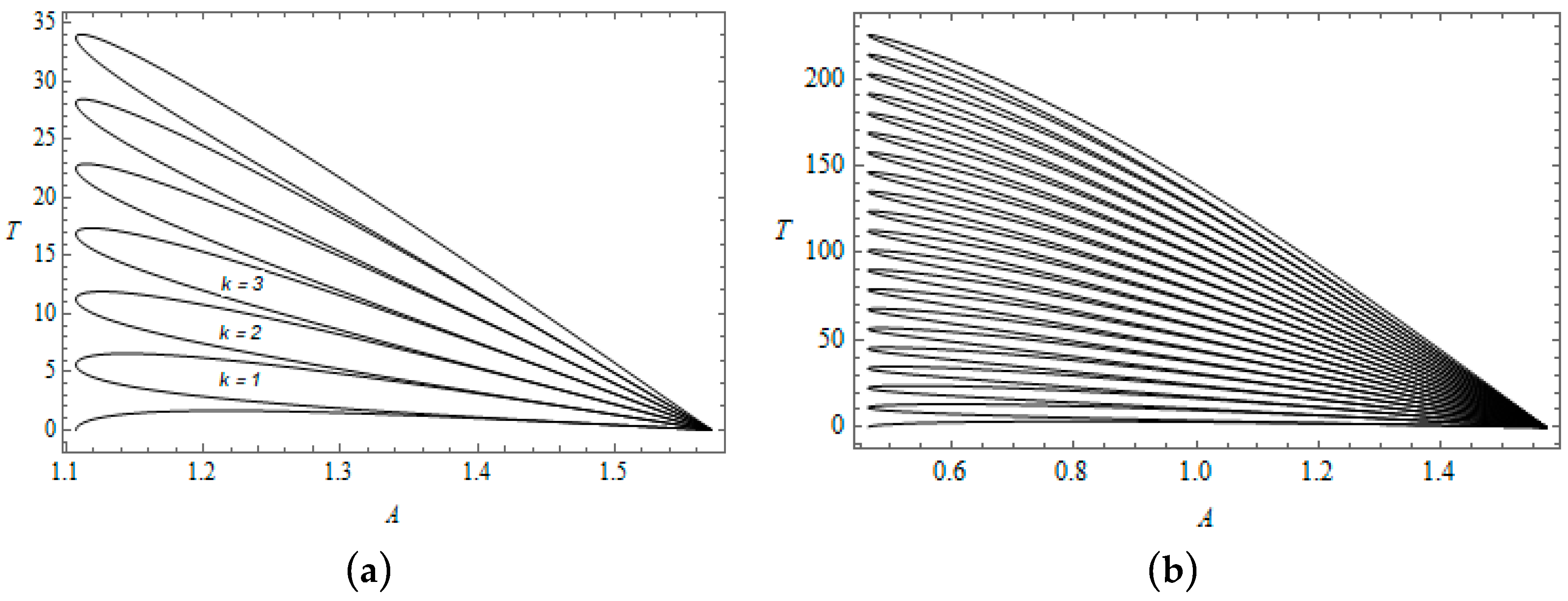
It can be shown that solutions (22) and (23) exist in the interval
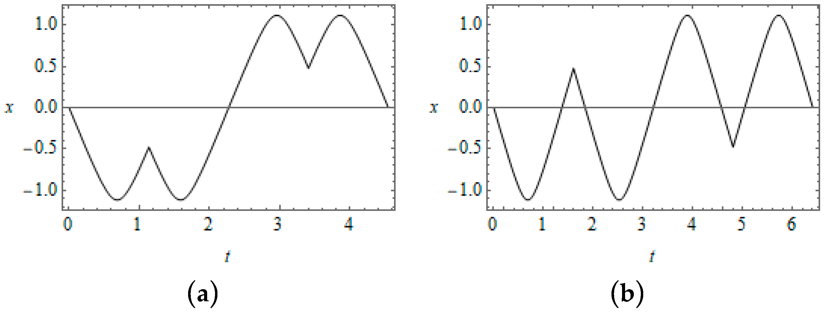
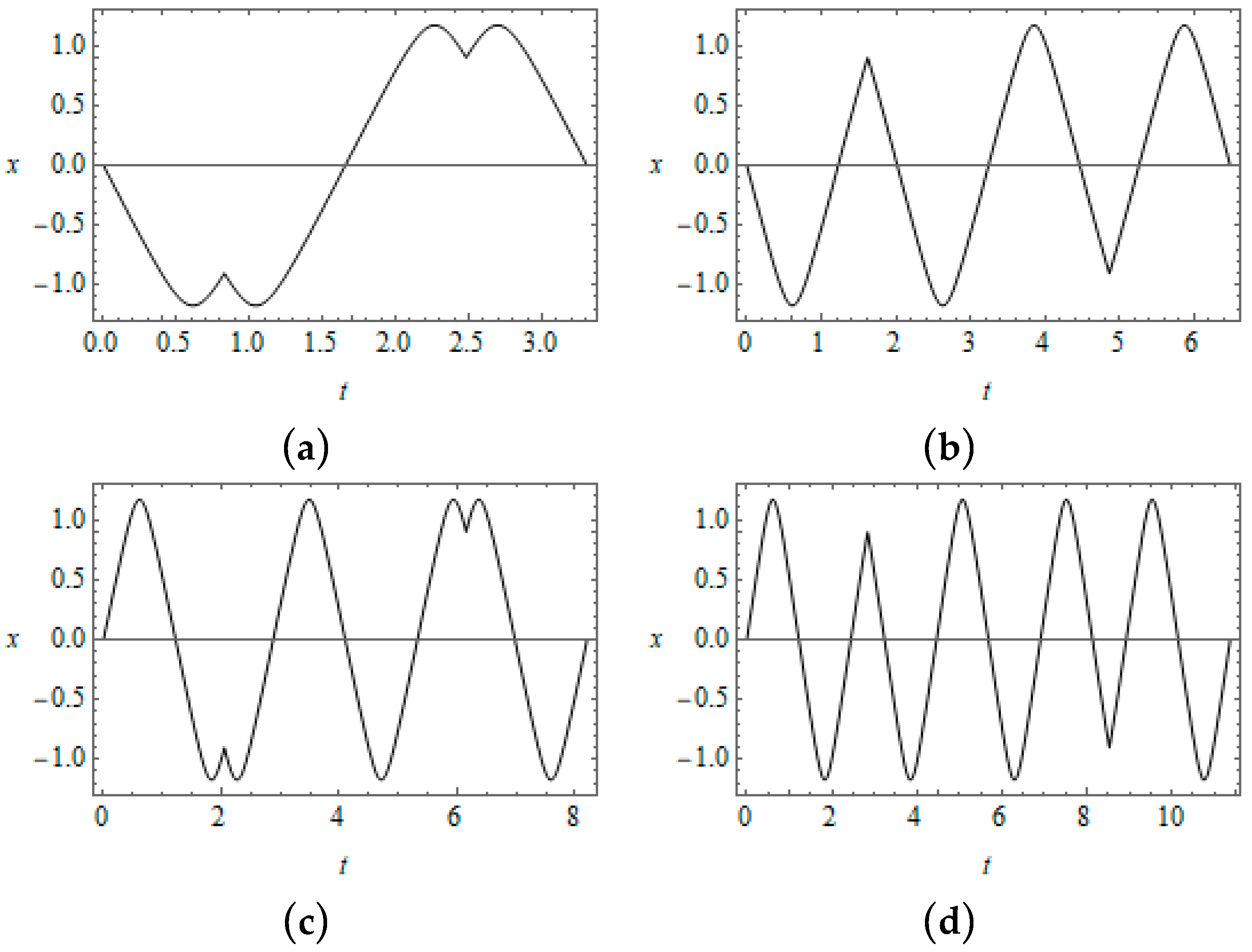
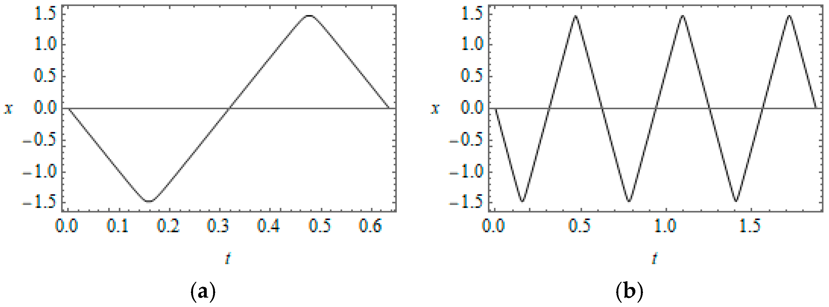
Figure 4 illustrates the sequence of branches of solutions (22) and (23) at different numbers under the fixed parameter of the strength of pulses, . The diagram reveals such combinations of the period and amplitude at which the oscillator has a periodic response with the loading period, . The upper and lower branches of each loop correspond to positive and negative signs in expression (22), respectively. In particular, relationship (23) corresponds to the number and has only the upper branch. For the selected value of , the minimal amplitude is , corresponding to the left boundary of the amplitude-period loops in Figure 4. A slight shift to the right from this boundary leads to bifurcations of solutions as seen from the time histories in Figure 5. The series of graphs illustrates only the first three couples of new solutions from the infinite set of solutions. Further evolution of the temporal shapes due to the amplitude increase is shown in Figure 6. One can observe quite a significant difference in both periods and temporal shapes of vibrations comparing the left and right fragments of Figure 6. This is explained by the high sensitivity of solutions near the left boundary with respect to the amplitude variation as follows from Figure 4. Finally, when the amplitude becomes close to its maximum , the restoring force of the oscillator itself generates quite strong pulses compared to the external loading as seen from the temporal mode shapes in Figure 7. As a result, the effect of external pulses is effectively vanishing. The oscillator’ response can be viewed rather as a free vibration whose amplitude and period are dictated by the loading period.
Analyzing the link between Figure 4 and Figure 5 shows that solutions corresponding to different loops of the period-amplitude dependence differ by the number of half cycles between any two consecutive pulses applied to the oscillator. These graphs were reproduced by solving the original equation numerically with the Mathematica® NDSolve package using the WhenEvent option for conditioning the velocity steps when passing the impulses under the initial conditions imposed by solution (24); see Appendix B for the code.
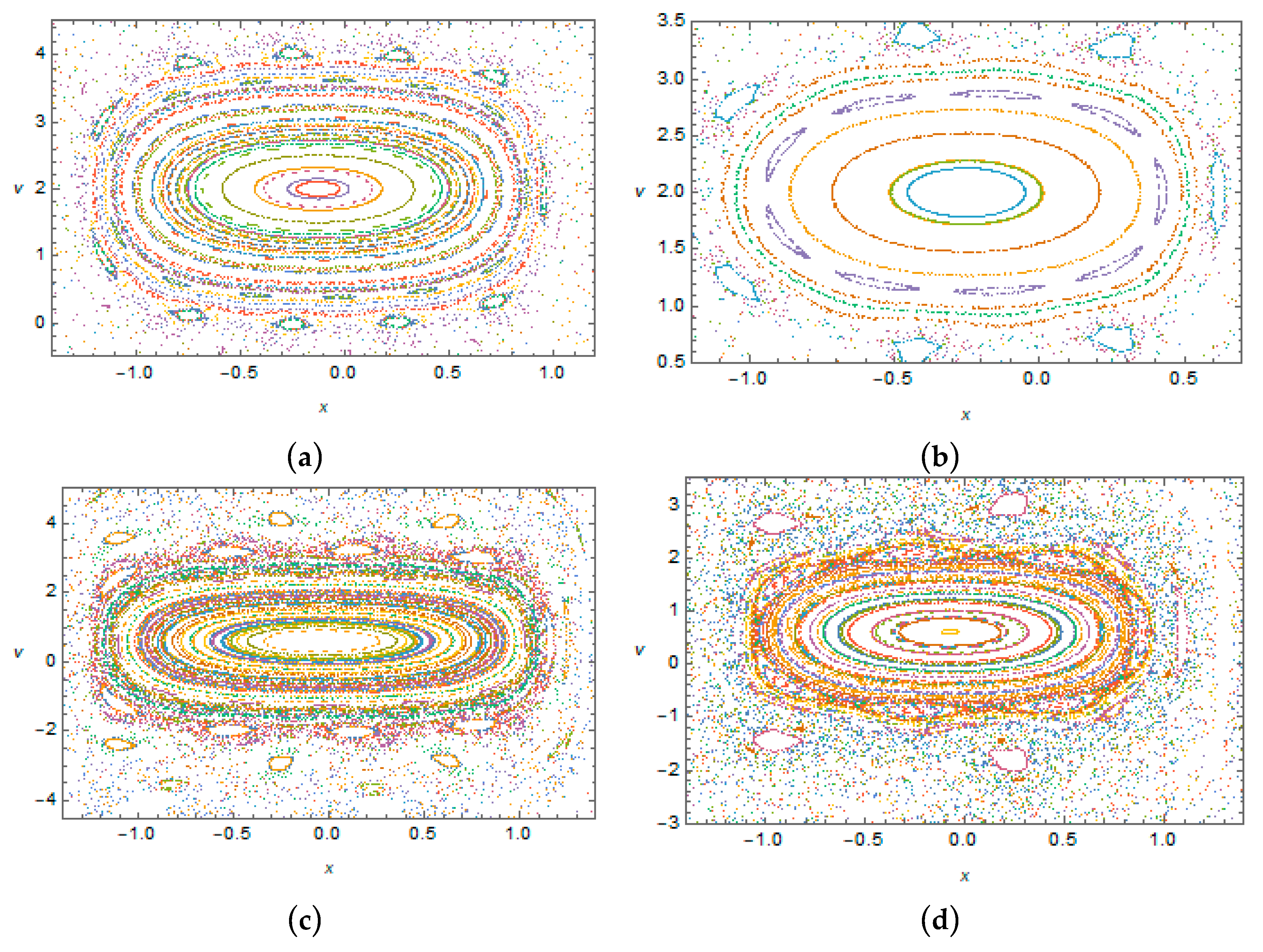
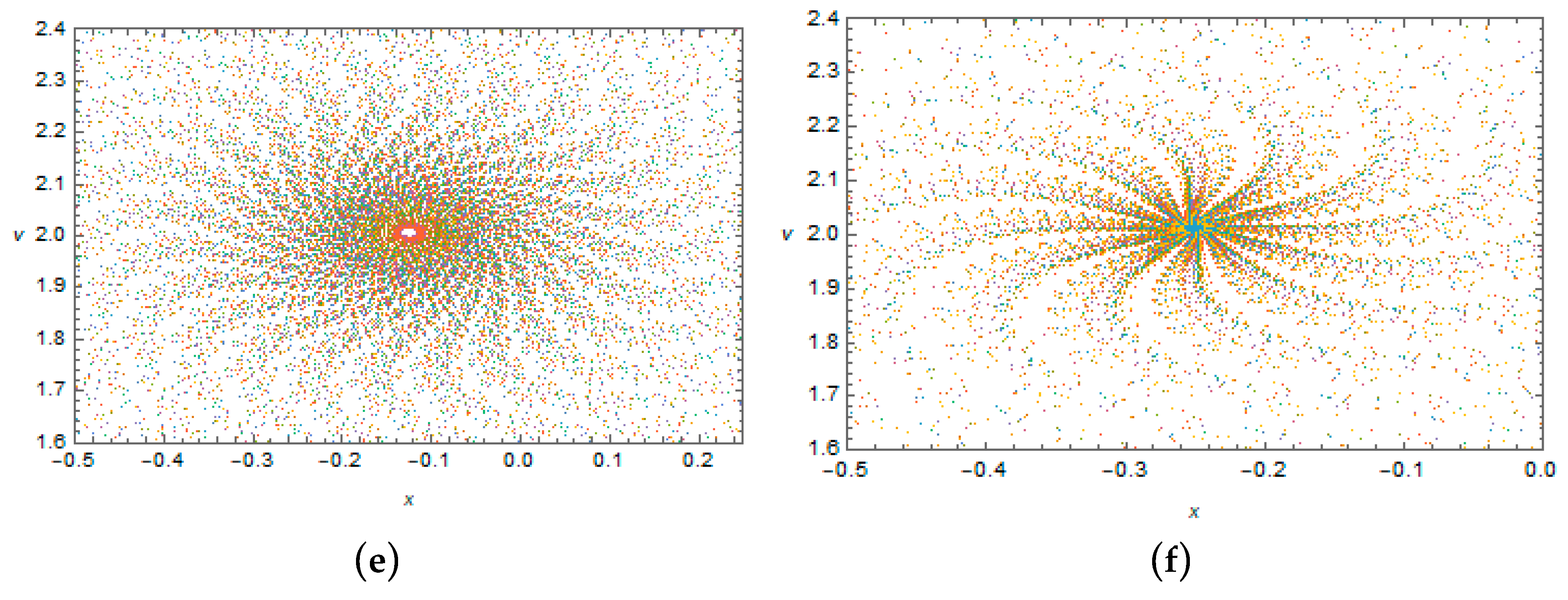
Note that, away from the curves of Figure 4, the response may appear to be quite complicated. This is confirmed by the Poincaré sections in Figure 8 and Figure 9 below. In particular, Figure 8 shows the Poincaré sections obtained for the case of short loading periods under a set of randomly chosen initial conditions. Then Figure 8a–d represents a weakly damped case, in which the energy inflow is sufficient for keeping the oscillator amplitudes large enough for a “resonance” interaction between the oscillator and the impulsive load. With the increase of dissipation, the initial energies of the oscillator dissipate leading to the decrease of its own frequencies. As a result, the high frequency impulsive loading becomes effectively quasi dynamic as reflected by the drastic change in Poincaré sections; see Figure 8e,f.
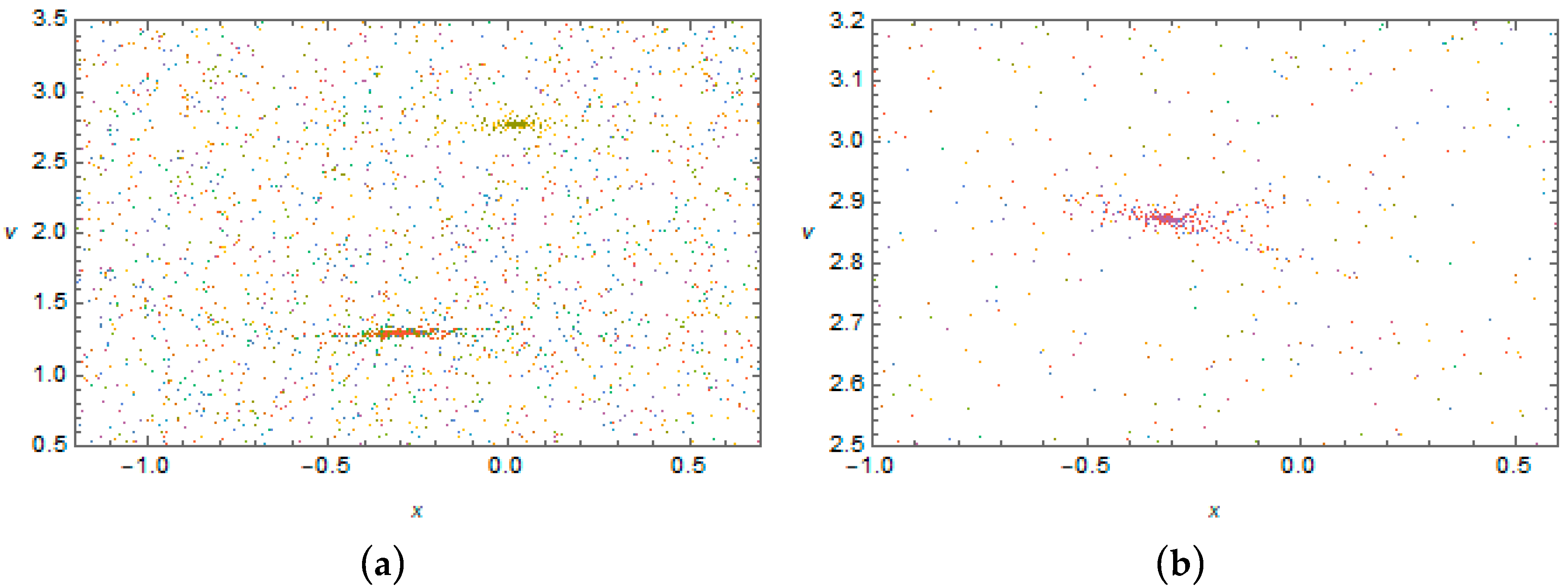
Finally, Figure 9 illustrates the case of a long-period impulsive loading under a relatively large damping, compared to the cases of Figure 8a–d. The difference between this case and the case represented by Figure 8e,f is that the distance between pulses is now long enough compared to the period of linearized oscillator whose period is the longest possible. As a result, the quasi dynamic branching in the Poincaré maps disappears.
3. Conclusions
Non-smooth temporal transformations are adapted for linear and nonlinear dynamical systems under discontinuous and impulsive periodic excitations. In particular, closed form analytical solutions for the strongly nonlinear exactly solvable oscillator are obtained. The solutions are represented by a family of period-amplitude dependencies with the corresponding time histories. Nonstationary responses under the presence of damping are illustrated by Poincaré sections at different magnitudes and periods of impulses. Practical importance of such a strongly nonlinear oscillator is due to the fact that the discontinuities of the restoring force characteristic can play the role of amplitude limiters without typical nonholonomic constraint conditions.
Funding
This research received no external funding.
Conflicts of Interest
The author declares no conflict of interest.
Appendix A. Proof of Identity (4)
Identity (4) was originally justified by the direct verification [3]. Now, following reference [8] and assuming , let us show that expression (4) can be produced by the temporal substitution
This relationship is obtained geometrically by combining the diagrams and of Figure 1 on the period . Note that discontinuity of the function at the point is suppressed by the continuous factor which takes zero value at the same point . Analogously, the relationship is considered to be true everywhere in the interval in algebraic manipulations with (A1). For example,
and thus
where is any positive integer, and are polynomials of the degree or .
Expression (A3) shows that any analytic function on the interval can be represented in the form
where and are power series of .
Now, let us assume that expression (A4) holds even though the function is not analytic. In this case, the question is whether or not it is possible to determine the components and without no power series expansions. The answer is positive. Namely, since either or on the entire interval , except may be for , then expression (A4) generates two equations and . Therefore, the components and are determined through and as
Therefore (A4) holds on the interval , except may be the point .
Now, if the function is continuous at then identity (A4) is also true at because
as .
If the function is periodic of the period then identity (51) holds for almost all , because the right-hand side of the identity depends on the time argument via the pair of periodic functions and of the same period .
If the function is continuous at then identity (A4) is true for all . Let us consider the point , where the function has a step-wise discontinuity. Note that another boundary, , is identical due to the periodicity. Taking into account that and the periodicity condition gives
Therefore, discontinuity of the function at the point is suppressed by zero factor
as provided that the function is continuous at the point .
So it is proved that identity (A4,A5) holds for all if the function is continuous.
If is not continuous then identity (A4) should be interpreted in the corresponding class of functions . For example, if the function is step-wise discontinuous at the time instances then the limits (A6) and (A8) become non-zero to represent the corresponding step-wise discontinuities of the function . In this case, the discontinuities of the function are not suppressed but describe the real behavior of the original function at the time instances .
Finally, if the period is then relationship (A1) must be modified as
Appendix B. Mathematica® Code Validating Solution (22)–(24)
The initial conditions {y0, v0} are imposed by solution (24) in order to provide periodicity. Note that the above fragment depicts the logic of solvers without strictly following the symbolic conventions of Mathematica® package.
References
- Filippov, A.F. Differential Equations with Discontinuous Right Hand Sides; Kluwer Academic Publishers Group: Dordrecht, The Netherlands, 1988. [Google Scholar]
- Fucik, S.; Kufner, A. Nonlinear Differential Equations; Elsevier: Amsterdam, The Netherlands; Oxford, UK; New York, NY, USA, 1980. [Google Scholar]
- Pilipchuk, V.N. Transformation of oscillating systems by means of a pair of non-smooth periodic functions. Dokl. Akad. Nauk Ukr. SSR Ser. A 1988, 4, 37–40. [Google Scholar]
- Pilipchuk, V.N. Nonlinear Dynamics: Between Linear and Impact Limits; Springer: Berlin, Germany, 2010. [Google Scholar]
- Kisil, V.V. Induced representations and hypercomplex numbers. Adv. Appl. Clifford Algebras 2013, 23, 417–440. [Google Scholar] [CrossRef]
- Kauderer, H. Nichtlineare Mechanik; Springer: Berlin/Heidelberg, Germany, 2013. [Google Scholar]
- Percival, I.C.; Richards, D. Introduction to Dynamics; Cambridge University Press: Cambridge, UK, 1982. [Google Scholar]
- Pilipchuk, V.N. Temporal transformations and visualization diagrams for non-smooth periodic motions. Int. J. Bifurc. Chaos 2005, 15, 1879–1899. [Google Scholar] [CrossRef]
Figure 1.
Non-smooth periodic basis.

Figure 2.
Geometrical interpretation of the particular case with a sine-wave temporal symmetry: observing the coordinate x does not reveal which of the two temporal variables, τ or t, is ‘in play’.
Figure 2.
Geometrical interpretation of the particular case with a sine-wave temporal symmetry: observing the coordinate x does not reveal which of the two temporal variables, τ or t, is ‘in play’.

Figure 3.
(a) Possible smooth fitting curve (20) approximating the restoring force of combined springs including the amplitude limiters, and (b) moving platform periodically strikes the perfectly stiff walls creating the impulsive inertia load on the oscillator in the moving noninertial frame; it is assumed that both spatial and temporal variables are appropriately scaled.
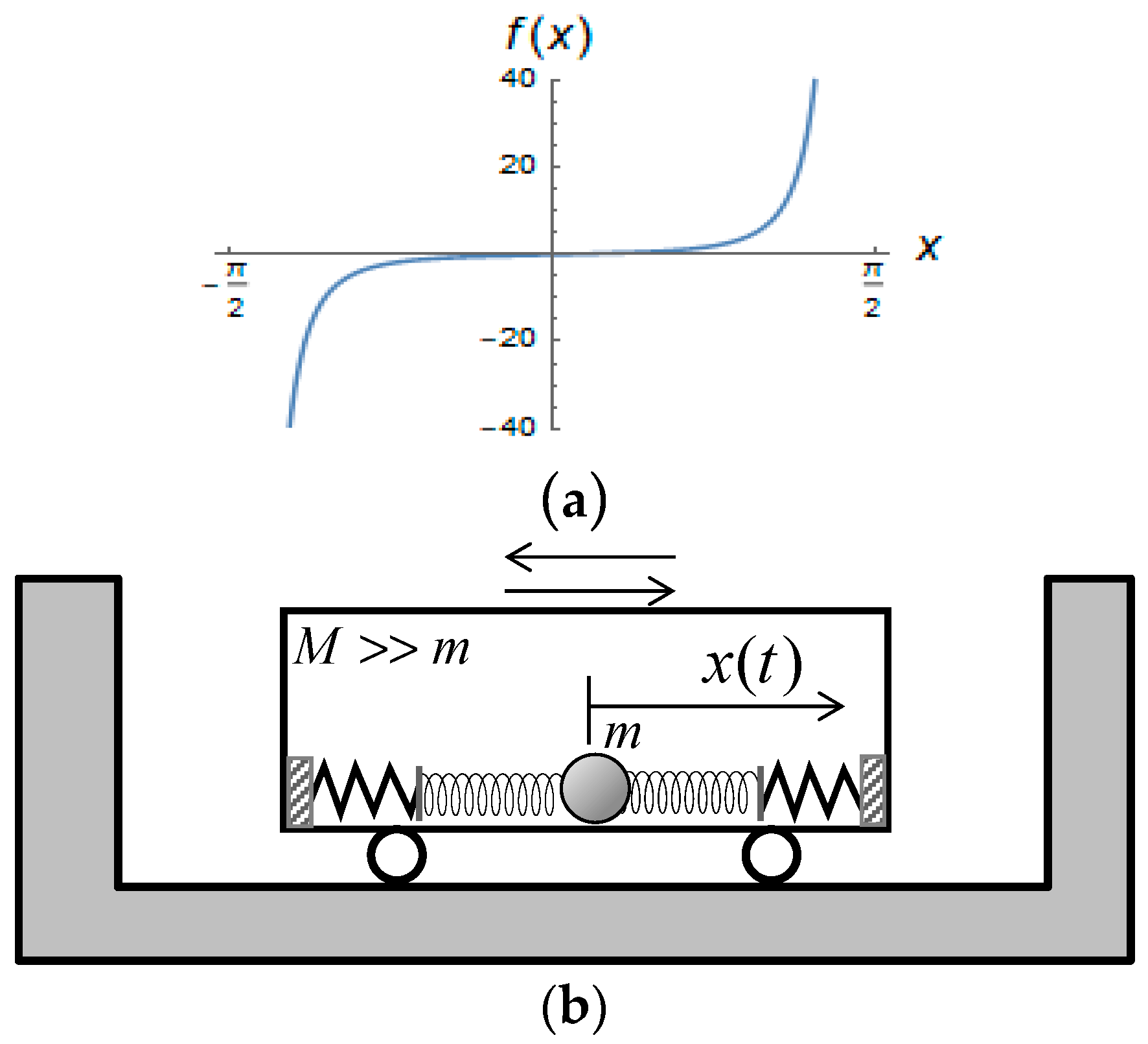
Figure 4.
First seven amplitude-period curves (22) and (23) of the oscillator at (a): , first seven branches are shown, and (b): , first 21 branches are shown.
Figure 4.
First seven amplitude-period curves (22) and (23) of the oscillator at (a): , first seven branches are shown, and (b): , first 21 branches are shown.

Figure 5.
Time histories of the oscillator’ response near the minimum amplitude parameter A = 1.12: k = 1 (a,b); k = 2 (c,d); k = 3 (e,f); the left and right columns correspond to the lower and upper branches of loops shown in Figure 4.
Figure 5.
Time histories of the oscillator’ response near the minimum amplitude parameter A = 1.12: k = 1 (a,b); k = 2 (c,d); k = 3 (e,f); the left and right columns correspond to the lower and upper branches of loops shown in Figure 4.

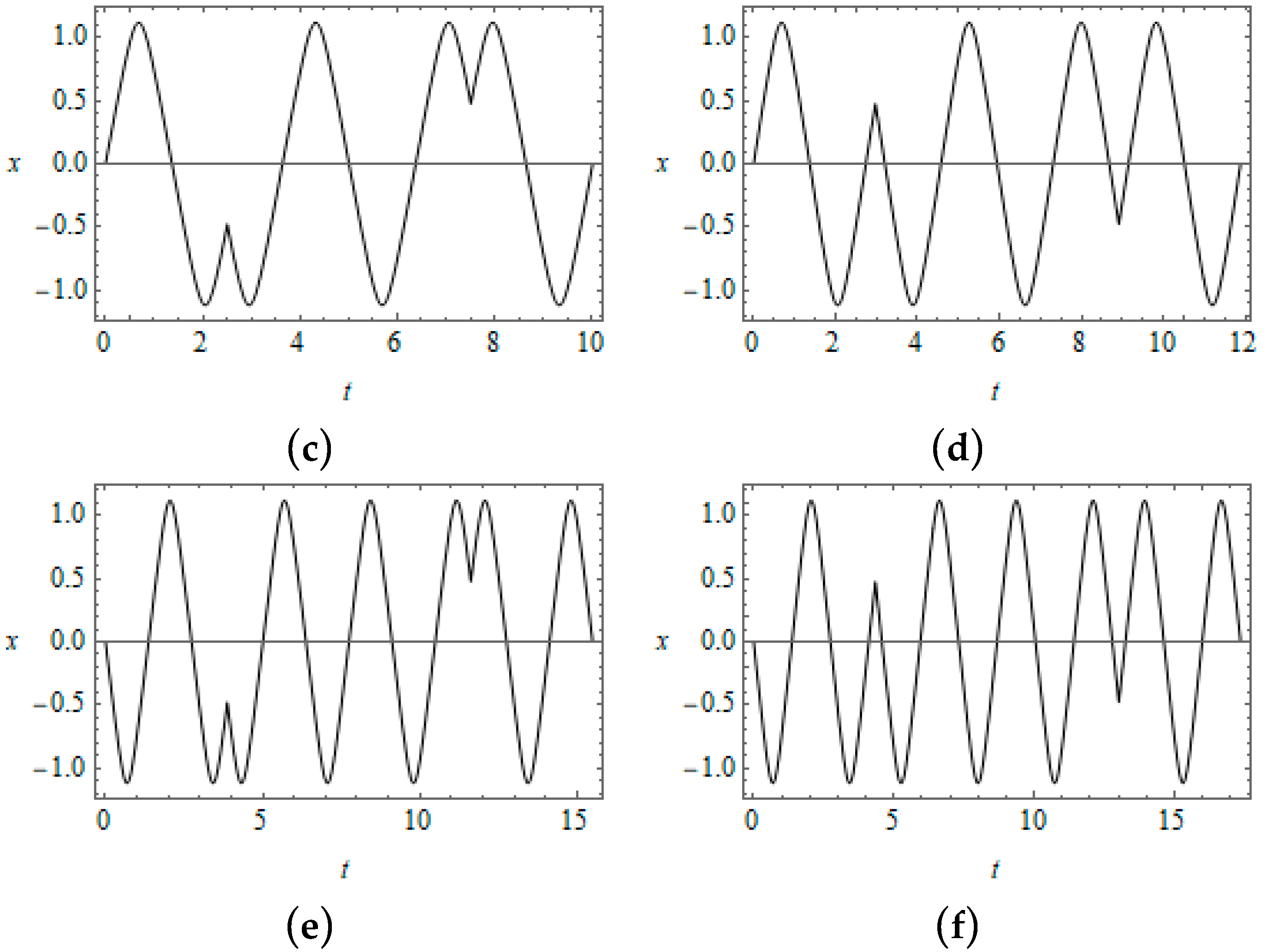
Figure 6.
Time histories of the oscillator’ response near the minimum amplitude parameter A = 1.1708: k = 1 (a,b); k = 2 (c,d); k = 3 (e,f); the left and right columns correspond to the lower and upper branches of the loops shown in Figure 4.
Figure 6.
Time histories of the oscillator’ response near the minimum amplitude parameter A = 1.1708: k = 1 (a,b); k = 2 (c,d); k = 3 (e,f); the left and right columns correspond to the lower and upper branches of the loops shown in Figure 4.

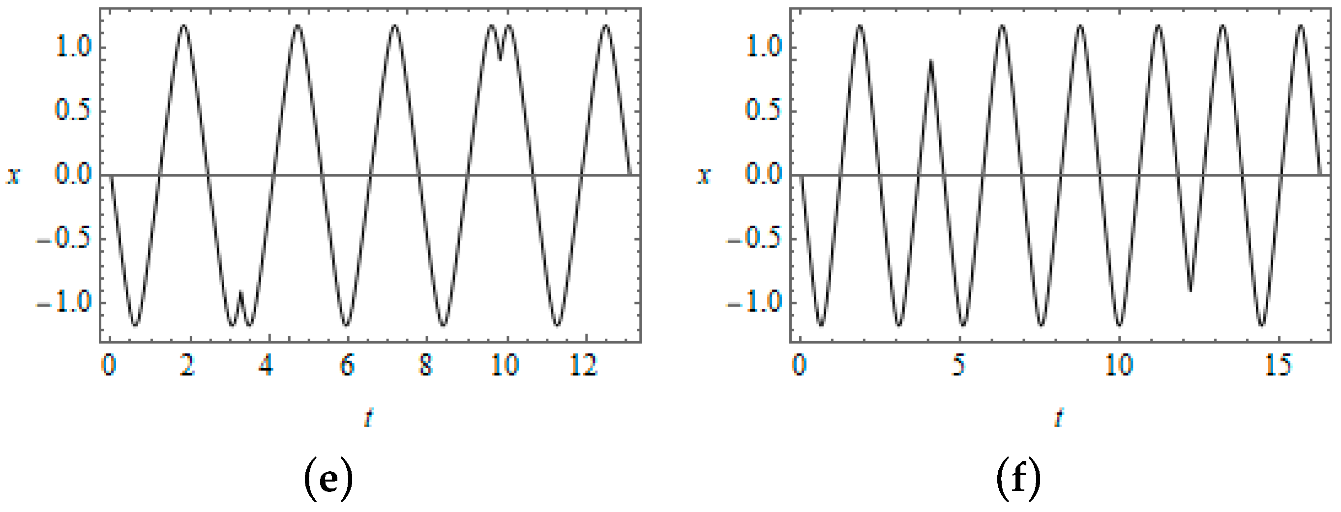
Figure 7.
Case k = 1, larger amplitude parameter A = 1.4708: (a) corresponds to the lower part of the loop, and (b) corresponds the upper part of the loop shown in Figure 4 for k = 1.
Figure 7.
Case k = 1, larger amplitude parameter A = 1.4708: (a) corresponds to the lower part of the loop, and (b) corresponds the upper part of the loop shown in Figure 4 for k = 1.

Figure 8.
Poincaré sections at (a): T = 0.25; F = 2.0; ζ = 0.0001, and (b): T = 0.5; F = 2.0; ζ = 0.0001; (c): T = 0.25; F = 0.6; ζ = 0.0001; (d): T = 0. 5; F = 0.6; ζ = 0.0001; (e): T = 0.25; F = 2.0; ζ = 0.05; (f): T = 0.5; F = 2.0; ζ = 0.05; snapshots are taken once per period at time of negative pulses.


Figure 9.
Poincaré sections at (a): T = 4.5; F = 2.0; ζ = 0.01, and (b): T = 8.5; F = 2.0; ζ = 0.01; snapshots are taken once per period at time of negative pulses.
Figure 9.
Poincaré sections at (a): T = 4.5; F = 2.0; ζ = 0.01, and (b): T = 8.5; F = 2.0; ζ = 0.01; snapshots are taken once per period at time of negative pulses.
© 2019 by the author. Licensee MDPI, Basel, Switzerland. This article is an open access article distributed under the terms and conditions of the Creative Commons Attribution (CC BY) license (http://creativecommons.org/licenses/by/4.0/).
Share and Cite
MDPI and ACS Style
Pilipchuk, V. Closed Form Solutions for Nonlinear Oscillators Under Discontinuous and Impulsive Periodic Excitations. Symmetry 2019, 11, 1420. https://doi.org/10.3390/sym11111420
AMA Style
Pilipchuk V. Closed Form Solutions for Nonlinear Oscillators Under Discontinuous and Impulsive Periodic Excitations. Symmetry. 2019; 11(11):1420. https://doi.org/10.3390/sym11111420
Chicago/Turabian StylePilipchuk, Valery. 2019. "Closed Form Solutions for Nonlinear Oscillators Under Discontinuous and Impulsive Periodic Excitations" Symmetry 11, no. 11: 1420. https://doi.org/10.3390/sym11111420
Note that from the first issue of 2016, this journal uses article numbers instead of page numbers. See further details here.