A Multi-Stage Homotopy Perturbation Method for the Fractional Lotka-Volterra Model
by
 , , and
Martin P. Arciga-Alejandre
 ,
,
Jorge Sanchez-Ortiz
*,
Francisco J. Ariza-Hernandez
and
Gabriel Catalan-Angeles
Facultad de Matemáticas, Universidad Autónoma de Guerrero, Av. Lázaro Cárdenas S/N Cd. Universitaria. Chilpancingo, Guerrero C.P. 39087, Mexico
*
Author to whom correspondence should be addressed.
Symmetry 2019, 11(11), 1330; https://doi.org/10.3390/sym11111330
Submission received: 21 September 2019
/
Revised: 22 October 2019
/
Accepted: 22 October 2019
/
Published: 24 October 2019
(This article belongs to the Special Issue Recent Advances in Discrete and Fractional Mathematics)
Abstract
:In this work, we propose an efficient multi-stage homotopy perturbation method to find an analytic solution to the fractional Lotka-Volterra model. We obtain its order of accuracy, and we study the stability of the system. Moreover, we present several examples to show of the effectiveness of this method, and we conclude that the value of the derivative order plays an important role in the trajectories velocity.
1. Introduction
The well-known predator-prey model was introduced by Lotka [1] and Volterra [2]. The resulting model is the classical Lotka-Volterra system of ordinary differential equations, which is proposed to provide a model for two-species competition. This model has potential applications in various fields of science like biology, sociology, medicine, history, economics, and ecology, among others. In addition, competition between more than two species has been studied in the field of mathematical biology using Lotka-Volterra-type systems, describing multispecies population dynamics. Many interesting results on the dynamical behavior for the solutions have been found in [3,4,5,6,7], such as the existence and uniqueness of solutions, asymptotic behavior, and bifurcations of the system.
On the other hand, fractional differential equations have been highly attractive to many scientists due to the fact that these equations have many applications in a wide range of phenomena (see [8,9,10,11,12,13]). In comparison with standard derivatives of integer order, the fractional order derivatives are characterized by their memory; i.e., the rate of change of a function near a point is affected by the history in the time domain of definition rather than just near the point itself.
In this note, we study the fractional Lotka-Volterra model
where a, b, c, and d are non-negative constants, , , and , and is the Caputo fractional derivative. Javeed et al. [14] use the homotopy perturbation method (HPM) (see [15]) to solve fractional partial differential equations. Rafei et al. [16], using HPM, found an approximation to the solution for the classic Lotka-Volterra model (). In addition, Kadem and Baleanu [17] use HPM to find an analytic approximate solution for the coupled Lotka-Volterra equations. On the other hand, HPM was implemented by Chowdhury et al. [18] to subintervals of equal length from a partition of total time evolution. This algorithm is known as the multistage homotopy perturbation method (MHPM). Moreover, the model (1) was studied by Das and Gupta [19] applying HPM, where the parameters , y d depend on time. However, its solution is valid only for a small time interval. Other numerical methods have been used to study nonlinear fractional differential equations (see [20,21,22]); for example, Pilar et al. [23], using Diethelm’s numerical algorithm, find solutions when and , .
In this work, we propose to implement an MHPM to the fractional Lotka-Volterra model defined in (1) in order to obtain an analytical solution for the model, and an expression for the truncation error is given. Through Lemma 2, the stability of the system is guaranteed, which is analogous to the results obtained by Ahmed et al. [8] and Elsadany et al. [9]. Finally, several examples are presented to show the effectiveness of this method.
2. Preliminaries
In this section, we give some basic definitions and properties of fractional calculus theory that are used in this work.
Definition 1.
The Riemann–Liouville fractional integral of order is defined by
where Γ is the gamma function.
It can be directly verified that
where .
Definition 2.
The Caputo fractional derivative of order is defined by
where , for and for .
Lemma 1.
Let and be a differentiable function in . Then .
Proof.
The proof can be found in [24]. □
Lemma 2.
We consider the fractional-order system
where . Suppose that m is the least common multiple of the denominators of , where for , and we set . System (3) is asymptotically stable at the equilibrium point if
for all roots λ of the following equation , and is the Jacobian matrix evaluated in , where .
Proof.
The proof can be found in [25]. □
3. Main Result
Theorem 1.
Let be a partition of , such that
and let , where , be solutions for the following initial value problems:
with and , for . Therefore, the solution for the system (1) is
where
Proof.
In order to solve (4) for each k, we apply the homotopy perturbation method (see [15]). First, we define the homotopy
where . Let us suppose that the solution to (4) is given by
where , are functions to be determined. Therefore, the solution will be
In order to find the functions and , since the Caputo’s fractional derivative of a constant is zero, and , we note that from the system (6), it follows that
Substituting (7) in the above system, we get
Then, matching the coefficients, we obtain the following differential equations for and :
and
Applying Lemma 1, we get explicit expressions for y . For example,
and
Therefore, from the above calculations, Equation (5) follows. □
Now, if we only take the first n terms for the series in (5), the order of accuracy for the solution is and , when , for and , respectively. That is,
Here, is the partition length.
Convergence
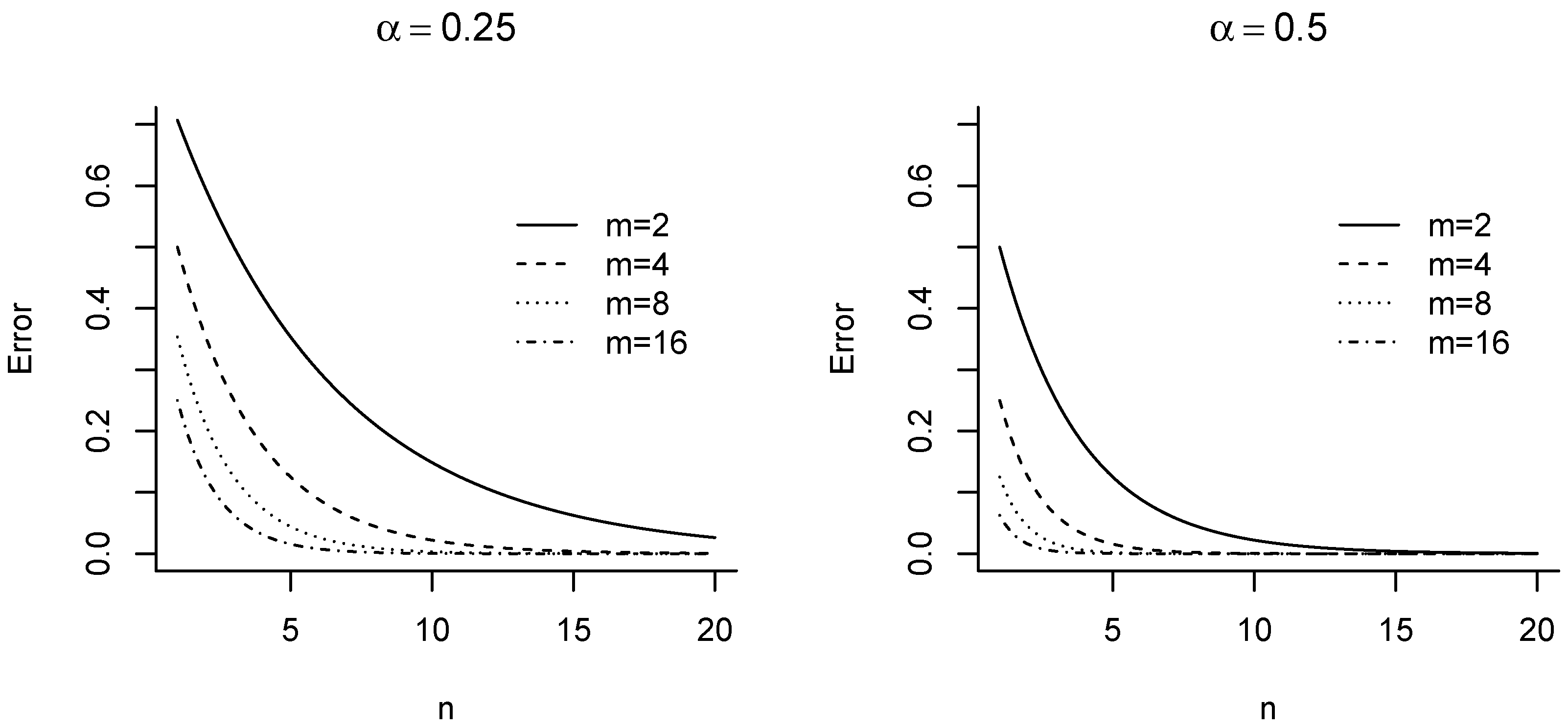
In order to demonstrate the efficiency of our method, we carry on an analysis of the series convergence for various values of the truncation parameters n and m that control the approximation accuracy. Here, the time step is , where T is the total length of the time interval (see Figure 1). We take as a reference value, and .
4. Examples
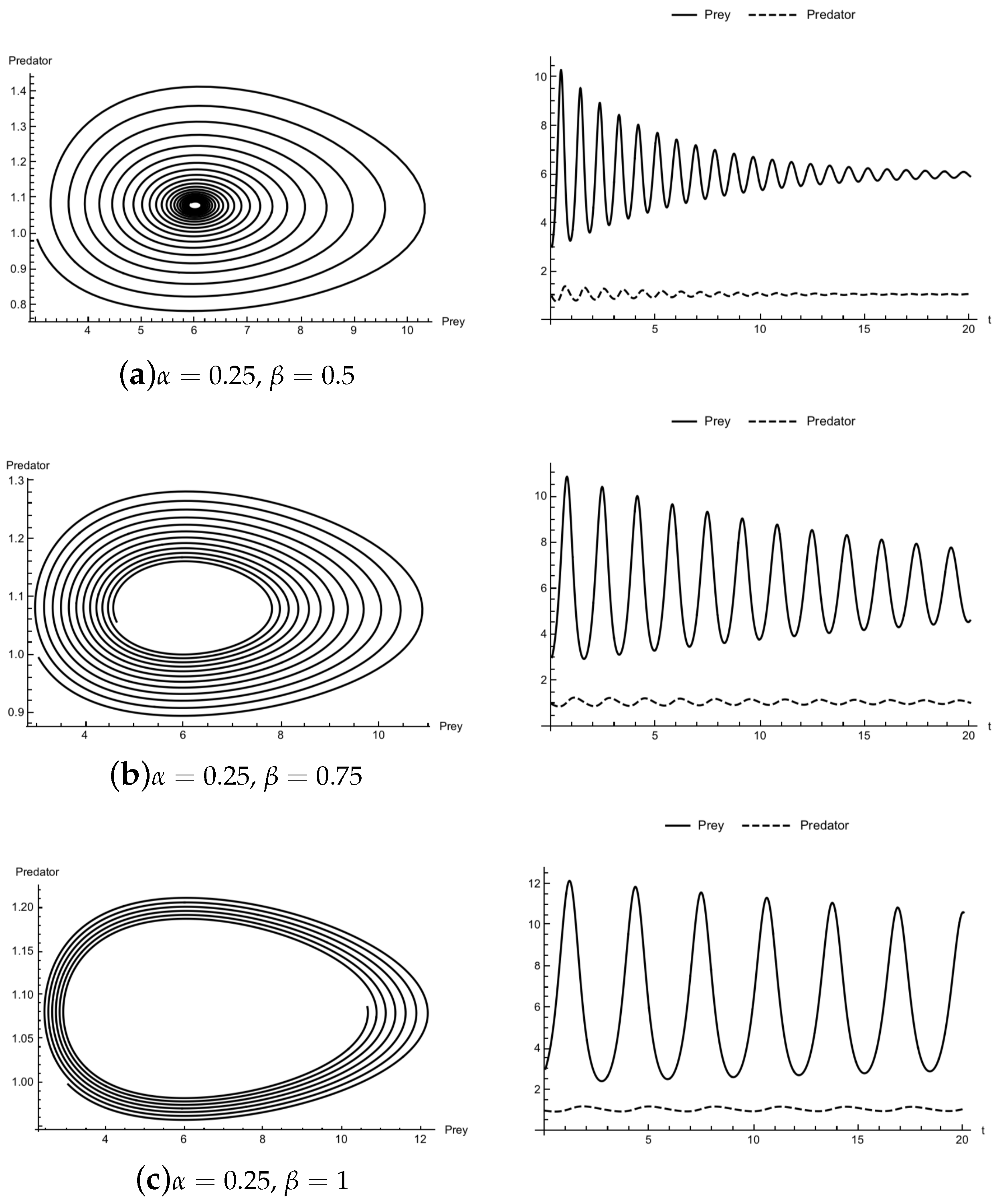
In order to illustrate the proposed method, we present some examples. Let be the initial condition, , , , , , and be the parameter values, , and . We consider the following cases for and .
Case 1.
taking the values 0.25, 0.5, 0.75, and 1.
Case 2.
fixed and β taking the values .
5. Conclusions
In this work, we found an analytic solution for a fractional Lotka-Volterra model using the multistage homotopy perturbation method. The effectiveness of this method is proven with different values for the parameters m, n, and . In Figure 1, we observe that for a given error, we can choose the partition size and the number of terms for the solution series. We note that when is getting close to zero, bigger values for m and n are needed in order to obtain a smaller error. From Figure 2, we conclude that the velocity trajectories depend of the fractional derivative order; if the order is close to zero, the trajectories get closer to the critical point faster. Moreover, we can observe that if and tend to one, the trajectories tend to be periodic, as in the classical case. In Figure 3, we take not equal to . A similar behavior to Case 1 is observed for the trajectories. In addition, lets point out that in the fractional Lotka-Volterra model, the solutions are not periodic. Then, the symmetry present in the ordinary case is broken when a fractional derivative is considered; this asymmetry is a typical feature of the fractional order systems of differential equations. Therefore, the model studied complements and generalizes the symmetric one. Finally, note that the behavior of the solutions depicted in Figure 1 and Figure 2 is consistent with the theoretical result given in Lemma 2.
Author Contributions
The authors contributed equally and significantly to writing this paper. All authors read and approved the final manuscript.
Funding
University of Guerrero, Mexico.
Conflicts of Interest
The authors declare that there is no conflict of interest regarding the publication of this paper.
Abbreviations
The following abbreviations are used in this manuscript:
| HPM | Homotopy perturbation method |
| MHPM | Multistage homotopy perturbation method |
References
- Lotka, A.J. Elements of Physical Biology; Williams and Wilkins: Baltimore, MD, USA, 1925. [Google Scholar]
- Volterra, V. Variazioni e fluttuazioni del numero di individui in specie animali conviventi. Mem. Acad. Lincei 1926, 2, 31–113. [Google Scholar]
- Ahmad, S.; Lazer, A.C. Average conditions for global asymptotic stability in a nonautonomous Lotka-Volterra system. Nonlinear Anal. Theory Methods Appl. 2000, 40, 37–49. [Google Scholar] [CrossRef]
- van den Driessche, P.; Zeeman, D.L. Three-dimensional competitive Lotka-Volterra systems with no periodic orbits. SIAM J. Appl. Math. 1998, 58, 227–234. [Google Scholar]
- Teng, Z.; Chen, L. Global asymptotic stability of periodic Lotka-Volterra systems with delays. Nonlinear Anal. Theory Methods Appl. 2001, 45, 1081–1095. [Google Scholar] [CrossRef]
- Lu, G.; Lu, Z. Permanence for two-species Lotka-Volterra cooperative systems with delays. Math. Biosci. Eng. 2008, 5, 477–484. [Google Scholar] [CrossRef]
- Chen, S.; Shi, J.; Wei, J. A note on Hopf birfucations in a delayed diffusive Lotka-Volterra predator-prey system. Comput. Math. Appl. 2011, 62, 2240–2245. [Google Scholar] [CrossRef]
- Ahmed, E.; El-Sayed, A.; El-Saka, A. Equilibrium points, stability and numerical solution of fractional-order predator-prey and rabies model. J. Math. Anal. Appl. 2007, 321, 542–545. [Google Scholar] [CrossRef]
- Elsadany, A.A.; Matouk, A.E. Dynamical behaviors of fractional-order Lotka-Volterra predator-prey model and its discretization. J. Appl. Math. Comput. 2015, 49, 269–283. [Google Scholar] [CrossRef]
- Bonilla, B.; Rivero, M.; Rodriguez, M.; Trujillo, J.J. Fractional differential equations as alternative models to nonlinear differential equations. Appl. Math. Comput. 2007, 187, 79–88. [Google Scholar] [CrossRef]
- Tenreiro Machado, J.A. (Ed.) Handbook of Fractional Calculus with Applications; De Gruyter: Berlin, Germany, 2019; Volumes 1–8. [Google Scholar]
- Napoles, J.E.; Rodriguez, J.M.; Sigarreta, J.M. New Hermite-Hadamard Type Inequalities Involving Non-Conformable Integral Operators. Symmetry 2019, 11, 1108. [Google Scholar] [CrossRef]
- Bisci, G.M.; Radulescu, V.D.; Servadei, R. Variational Methods for Nonlocal Fractional Problems; Encyclopedia of cs and its Applications; Cambridge University Press: Cambridge, UK, 2016; Volume 162. [Google Scholar]
- Javeed, S.; Baleanu, D.; Waheed, A.; Shaukat Khan, M.; Affan, H. Analysis of Homotopy Perturbation Method for Solving Fractional Order Differential Equations. Mathematics 2019, 7, 40. [Google Scholar] [CrossRef]
- He, J.H. Homotophy Perturbation Technique. Comput. Methods Appl. Mech. Eng. 1999, 178, 257–262. [Google Scholar] [CrossRef]
- Rafei, M.; Daniali, H.; Ganji, D.D.; Pashaei, H. Solution of the prey and predator problem by homotophy perturbation method. Appl. Math. Comput. 2007, 188, 1419–1425. [Google Scholar]
- Kadem, A.; Baleanu, D. Homotopy pertubation method for the coupled fractional Lotka-Volterra equations. Rom. J. Phys. 2011, 56, 332–338. [Google Scholar]
- Chowdhury, M.S.H.; Hashim, I.; Roslan, R. Simulation of the predator-prey problem by the homotopy-perturbation method revised. J. Juliusz Schauder Center 2008, 31, 263–270. [Google Scholar]
- Das, S.; Gupta, P.K. A mathematical model on fractional Lotka-Volterra equations. J. Theor. Biol. 2011, 277, 1–6. [Google Scholar] [CrossRef]
- Dhaigude, D.B.; Birajdar, G.A. Numerical solution of fractional partial differential equations by discrete Adomian decomposition method. Adv. Appl. Math. Mech. 2014, 6, 107–119. [Google Scholar] [CrossRef]
- Muhammed, I.S.; Mohammed, A.O. A Numerical Method for Solving a Class of Nonlinear Second Order Fractional Volterra Integro-Differntial Type of Singularly Perturbed Problems. Mathematics 2018, 6, 48. [Google Scholar] [CrossRef]
- Pitolli, F. A Fractional B-spline Collocation Method for the Numerical Solution of Fractional Predator-Prey Models. Fractal Fract. 2018, 2, 13. [Google Scholar] [CrossRef]
- Pilar, M.; Trujillo, J.J.; Luis, V.; Rivero, M. Fractional dynamics of populations. Appl. Math. Comput. 2011, 218, 1089–1095. [Google Scholar]
- Kilbas, A.A.; Srivastava, H.M.; Trujillo, J.J. Theory and Applications Fractional Differential Equations; Elsevier: San Diego, CA, USA, 2006. [Google Scholar]
- Tavazoei, M.S.; Haeri, M. Chaotic attractors in incommensurate fractional order systems. Phys. D 2008, 237, 2628–2637. [Google Scholar] [CrossRef]
Figure 1.
Convergence error.


Figure 2.
Case 1.
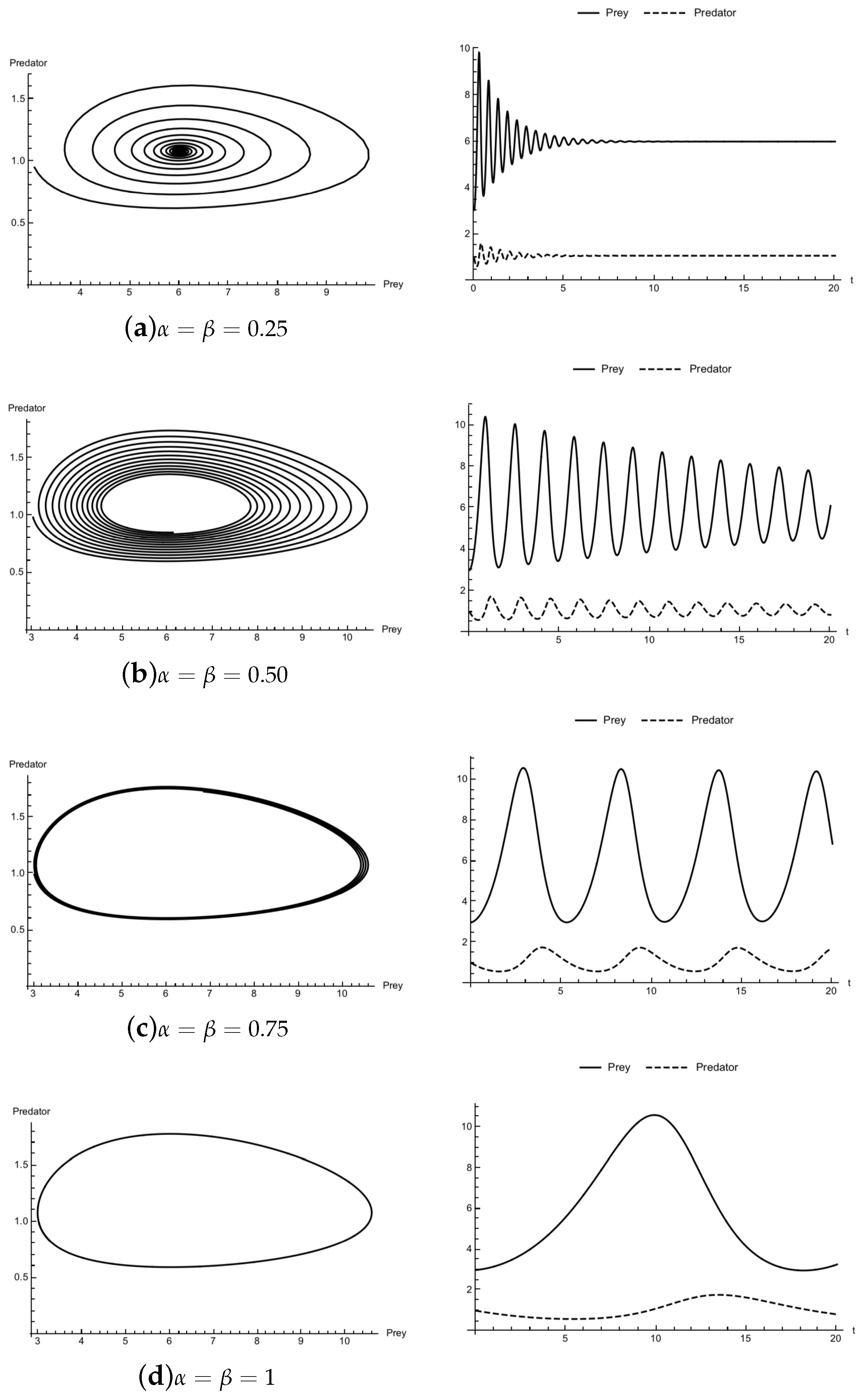
Figure 3.
Case 2.

© 2019 by the authors. Licensee MDPI, Basel, Switzerland. This article is an open access article distributed under the terms and conditions of the Creative Commons Attribution (CC BY) license (http://creativecommons.org/licenses/by/4.0/).
Share and Cite
MDPI and ACS Style
Arciga-Alejandre, M.P.; Sanchez-Ortiz, J.; Ariza-Hernandez, F.J.; Catalan-Angeles, G. A Multi-Stage Homotopy Perturbation Method for the Fractional Lotka-Volterra Model. Symmetry 2019, 11, 1330. https://doi.org/10.3390/sym11111330
AMA Style
Arciga-Alejandre MP, Sanchez-Ortiz J, Ariza-Hernandez FJ, Catalan-Angeles G. A Multi-Stage Homotopy Perturbation Method for the Fractional Lotka-Volterra Model. Symmetry. 2019; 11(11):1330. https://doi.org/10.3390/sym11111330
Chicago/Turabian StyleArciga-Alejandre, Martin P., Jorge Sanchez-Ortiz, Francisco J. Ariza-Hernandez, and Gabriel Catalan-Angeles. 2019. "A Multi-Stage Homotopy Perturbation Method for the Fractional Lotka-Volterra Model" Symmetry 11, no. 11: 1330. https://doi.org/10.3390/sym11111330
Note that from the first issue of 2016, this journal uses article numbers instead of page numbers. See further details here.