Quantification of Erosion in Selected Catchment Areas of the Ruzizi River (DRC) Using the (R)USLE Model


1
Institute of Physical Geography, Geo-Center of the Goethe University Frankfurt, Altenhöferallee 1, 60438 Frankfurt am Main, Germany
2
Unité d’Enseignement et de Recherche en Hydrobiologie Appliquée (UERHA), Institut Supérieur Pédagogique (ISP) de Bukavu, 32, Avenue Kibombo, Ibanda, B.P. 854 Bukavu, Democratic Republic of the Congo
3
Centre de Recherche en Environnement et Géoressources, Université Catholique de Bukavu (UCB), 2, Avenue de la Mission (Bugabo), B.P. 285 Bukavu, Democratic Republic of the Congo
*
Author to whom correspondence should be addressed.
Land 2020, 9(4), 125; https://doi.org/10.3390/land9040125
Submission received: 25 March 2020
/
Revised: 16 April 2020
/
Accepted: 21 April 2020
/
Published: 23 April 2020
(This article belongs to the Section Soil-Sediment-Water Systems)
Abstract
:Inappropriate land management leads to soil loss with destruction of the land’s resource and sediment input into the receiving river. Part of the sediment budget of a catchment is the estimation of soil loss. In the Ruzizi catchment in the Eastern Democratic Republic of the Congo (DRC), only limited research has been conducted on soil loss mainly dealing with local observations on geomorphological forms or river load measurements; a regional quantification of soil loss is missing so far. Such quantifications can be calculated using the Universal Soil Loss Equation (USLE). It is composed of four factors: precipitation (R), soil (K), topography (LS), and vegetation cover (C). The factors can be calculated in different ways according to the characteristics of the study area. In this paper, different approaches for calculating the single factors are reviewed and validated with field work in two sub-catchments of Ruzizi River supplying the water for the reservoirs of Ruzizi I and II hydroelectric dams. It became obvious that the (R)USLE model provides the best results with revised R and LS factors. C factor calculations required to conduct a supervised classification using the Maximum Likelihood Procedure. Different C factor values were assigned to the land cover classes. The calculations resulted in a soil loss rate for the predominantly occurring Ferralsols and Leptosols of around 576 kt/yr in both catchments, when 2016 landcover and precipitation are used. This represents an area-normalized value of 40.4 t/ha/yr for Ruzizi I and 50.5 t/ha/yr for Ruzizi II due to different landcover in the two sub-catchments. The mean value for the whole study area is 47.8 t/ha/yr or even 27.1 t/ha/yr when considering land management techniques like terracing on the slopes (P factor). This work has shown that the (R)USLE model can serve as an easy to handle tool for soil loss quantification when comprehensive field work results are sparse. The model can be implemented in Geographic Information Systems (GIS) with free data; hence, a validation is crucial. It becomes apparent that the use of high resolution Sentinel 2a MSI data as the basis for C factor calculations is an appropriate method for considering heterogeneous Land Use Land Cover (LULC) patterns. To transfer the approach to other regions, the calculation of factor R needs to be modified.
1. Introduction
Even if soil erosion can be easily defined as the displacement of soil particles from one location to another, its quantification in terms of soil loss for a respective area could be very complex due to five characteristics: the intensity of rainfall (erosivity), the soil type (erodibility), the land cover, the slope length and the slope steepness [1,2,3]. In the tropics, soil erosion mainly occurs as sheet and rill erosion triggered by overland flow [4].
Usually, soil erosion can be calculated by field measurements. Based on erosion plots at sites of different land use, soil patterns, and slope angles, precipitation and the amount of eroded material is measured over a minimum period of two years (for an example of an experimental setup at sites in Southern Cameroon, see Ambassa-Kiki and Nill [5]; for a detailed overview of erosion in the humid tropics, see Labrière et al. [6]). The measured erosion rates are extrapolated to catchment size using models based on high resolution soil maps, Digital Elevation Models (DEMs) and precipitation data [7].
A broad number of such models exist which model soil erosion as a whole or as a part of more complex models which are the Universal Soil Loss Equation (USLE; [1]) and its variations (Revised [R]USLE, Modified [M]USLE), the Agricultural Non-Point Source model (AGNPS), the Areal Non-point Source Watershed Environment Response System (ANSWERS) and the Chemicals, Runoff and Erosion from Agricultural Management Systems (CREAMS), both of which were discussed by Wu et al. [8]; the Groundwater Loading Effects of Agricultural Management Systems (GLEAMS), the Erosion Productivity Impact Calculator (EPIC) and the Water Erosion Prediction Project (WEPP), which were compared with RUSLE by Reyes et al. [9]. Chandramohan et al. [10] tested the Unit Sediment Graph (USG), the WEPP, and the RUSLE on small-scale Indian catchments of around 40 km² each. Their main objective was to predict the soil loss for six different extreme events with the respective parameters measured in the field. Four further events were measured to validate the model. As a result they recommend the USG model which fits best into their set up. However, the more general approach with freely available (global) data was not considered by them. Hrissanthou [11] figured out that the MUSLE is the best indicator for predicting the sediment yield and the Agriculture Research Service of the US (ARS) have recommended the RUSLE to assist public policy development all over the world [12]. It seems that USLE and its related concepts are powerful but controversially discussed tools.
Since 1978, USLE has been used by several researchers to estimate soil erosion and sediment yield [13] “because of its simplicity” as stated by Sotiropoulou et al. [14], although it considers also the “spatial heterogeneity of soil erosion” [15]. It is an equation that considers the main parameters influencing erosion, such as rainfall (R factor), soil (K factor), topography (LS factor), land cover (C factor), and land management (P factor), and was developed by Wischmeier and Smith [1]. Due to the complexity of the data incorporated in the model, different approaches are used for factor calculations: e.g., the R factor can be based on mean annual precipitation [16,17,18,19], mean monthly precipitation [15,20], or single daily events [13], though the use of mean annual precipitation probably leads to under-estimations of soil loss when there are distinct differences between rainy and dry season; the K factor uses predefined values according to soil types and/or colors [17,21] or on detailed grain size and carbon amount data [16,20]; or the C factor can be based on calculations of the Normalized Difference Vegetation Index (NDVI) [16,22] or again based on predefined values matched with land cover classes [17,21,23,24,25] (see Table A1, Table A2 and Table A3 for selected calculations and [3] for a (R)USLE review). The differences between USLE, RUSLE, and MUSLE depend on the calculation of the single factors, which have to be adapted to different climate, topography, and also research objectives [3]. For example in MUSLE, the rainfall factor is replaced by a runoff factor reflecting the “variability of deliver ratio” and therefore detailed precipitation data and outflow measurements are necessary [13]. Unfortunately, in most developing countries, erosion plot data are missing and weather or sediment load measurements are inconsistently dependent on the political situation in those countries and budget decisions, respectively. Considering that the recent history of the study area in Eastern Congo / the South Kivu Province is characterized by civil war and atrocities (e.g., the genocide in Rwanda and its following conflicts at the border to the DRC) bad data availability from these areas is understandable.
In this context, Karamage et al. [16] used USLE to model soil erosion for Lake Kivu catchment without any plot measurements in the field. According to the high relief energy, they modified the original equation for the topography (LS) developed by Desmet and Govers [26] to also consider the upstream contribution area for complex slopes. For the slope steepness factor, they used the formula based on McCool et al. [27], who differentiated between slope angles that were less and more than 9% to also consider steep angles along the East African Rift. For validation, they compared their results with a work of Bewket and Teferi [17], who used the model in an Ethiopian catchment in the upper Nile Basin. Karamage et al. [16] tested the model to examine different conservation practices along the steep slopes of Lake Kivu. They calculated a mean annual erosion risk of 3 kt/km² (30 t/ha) and only 33% of their study area has a tolerable soil loss of ≤ 1 kt/km². The main contributor to soil loss in this area is the cropland; therefore, they suggested adjusting the land use techniques to consider terracing, strip-cropping, and contouring.
For the Bukavu region, mainly gray literature deals with soil erosion (e.g., [28]) and its anthropogenic impacts (e.g., [29]) conducted for short periods in the framework of student projects. An area-wide quantification of soil erosion does not currently exist.
The main goal of this paper is therefore to (15) quantify the potential soil loss in the Ruzizi sub-catchments of hydropower plants Ruzizi I and II. In addition to the rates of loss, (2) the main sources of sediment input will be identified. We decided to use the (R)USLE model with K, LS, and P factors based on Karamage et al. [16] but modified R and C factors adjusted to the seasonality [15,20] and the heterogeneous and small scale land use practices in the region [16,17,23]. The study area of Karamage et al. [16] also covers small areas of the Ruzizi catchment directly at the outlet of Lake Kivu; therefore, it could be used for validation. Additionally, (3) aims to prove whether there are possibilities to validate the model beyond their work.
The results of soil loss quantification will be incorporated into the project “Environmental flow requirements of two dammed tropical rivers of the Congo Basin (Eastern Democratic Republic of Congo)” dealing with the impact of Ruzizi I and II hydroelectric dams on the freshwater ecosystem of Ruzizi River. This project aims to assess environmental flow requirements [30,31,32] in order to suggest optimum water resource use and obtain insights to enhance the sustainability of future dam construction. The central goal of the geomorphological sub-project is to estimate the sediment budget of the sub-catchments, and the (R)USLE results are an important component of these estimations.
2. Materials and Methods
2.1. Study Area
Ruzizi River is the outflow of Lake Kivu and is one of the major tributaries of Lake Tanganyika in the Congo catchment. Its basin covers an area of about 5800 km² [33]. It partially follows the East African Rift System in a steep valley before crossing the Ruzizi plains. The river connects Lake Kivu in the North and Lake Tanganyika in the South. From Lake Tanganyika there is an overflow to the West flowing into the Lualaba, which is the main headstream of the Congo River (see Figure 1). The study area is characterized by a steep relief with altitudes between 774 m a.s.l. at Lake Tanganyika, 1460 m a.s.l. at the coast of Lake Kivu, and 3308 m a.s.l. at Mont Kahuzi, the highest mountain in the region. The relief has its origin in the East African Rift, a graben system which has been active for 30 million years. The drainage network follows these tectonic lines. Along the structure, active volcanoes also exist [34] and earthquakes lead to frequent landslides in the region [35]. The geology is mainly composed of basaltic rocks from the Cenozoic age. Cenozoic sediments were deposited in the valley of Ruzizi River with a large accumulation at its mouth into Lake Tanganyika. There are also metasediments and Precambrian gneisses on its southern slopes [36]. On the basaltic rocks near Bukavu, Ferralsols were developed, which are depleted soils that are highly resistant against erosion. Large parts of the catchment area are covered by Leptosols and Umbrisols on the steep slopes directly over the basement rocks and rock fragments. At the delta-like outlet of the Ruzizi River Gleysols develop, which are used for agriculture in combination with an appropriate drainage system ([36]; see [37] for Food and Agriculture Organization [FAO] nomenclature). The climate is characterized by a bimodal system with two rainy and two dry seasons: The main rainy season lasts from February to May and the smaller one lasts from September to December; the main dry season lasts from June to August and the smaller one is in February [38]. However, the small dry season is still characterized by abundant precipitation of 120 mm in contrast to 20 mm in July and therefore should be called an intermediate season. The mean annual precipitation amounts to 1277 mm and the mean annual temperature is 20.3 °C [39]. The natural vegetation is mainly characterized by mountain rainforest in the mountainous area, as well as Miombo and savanna woodland in the lower and flat parts along the Ruzizi Plains [40]. However, based on Hansen et al. [41,42] the Ruzizi catchment had a forest cover of 2350 km² in 2000 and a forest loss of 53.16 km² from 2000 to 2014. Parts of this loss can be matched to infrastructure and irrigation projects but it is mostly due to burning activity, which is still a common way for pastoralists to cause grasses to sprout.
The northern part of the river represents the border between Rwanda and the DRC. As a result of the Rwandan genocide, war and insecurity in the region increased, accompanied by an escape of rural populations to the larger towns. Bukavu is the capital of South Kivu province with a number of inhabitants estimated at 950,000 in 2013 [43]. The relief forces people to also settle on steep slopes or in alluvial plains. Agriculture is conducted close to their huts. Both settling and conducting agricultural activities in such a relief under a humid climate lead to high erosion and landslides.
Due to its steep relief, the Ruzizi River is appropriate for hydroelectric dams with relatively small dams and reservoirs. Dam Ruzizi I was constructed just before independence obtained by the DRC in 1959, with a capacity of 29.8 MW. It is situated at the outlet of Lake Kivu close to Bukavu. In 1989, Ruzizi II was constructed with a capacity of 43.8 MW about 15 km downstream of Ruzizi I [44].
Within the Ruzizi catchment, the sub-catchments of dams Ruzizi I and II cover an area of 32 km² and 90 km², respectively [33]. Around 10% of Ruzizi I catchment is located on the Congolese side, which is mainly characterized by the sealed surface of Bukavu town. The rest of the area is on the Rwandan side and is mainly surrounded by cropland and a few settlements. For Ruzizi II, around 60% of the catchment is located on the Congolese side with a transitional zone from densely populated Bukavu to a more agricultural area with a few banana tree plantations and islands of forest. On the Rwandan side, the area is characterized by cropland; hence during field work, terraces could be observed along the steep slopes. This is in contrast to the Congolese side, where are a small number of gullies that are deeply incised small-scale erosional features occurring in the study area due to the prolongation of sewage channels.
2.2. Implementation of Freely Available Datasets into (R)USLE
The Universal Soil Loss Equation (USLE) was developed “to compute longtime average soil losses from sheet and rill erosion” while considering “numerous physical and management variables” [1]. The factors of the equation are the rainfall and runoff factor (R), soil erodibility factor (K), topographic factor (LS), cover and management factor (C), and support practice factor (P). The product of all factors is the proposed amount of soil loss per hectare per year in tons called A (Equation (1)).
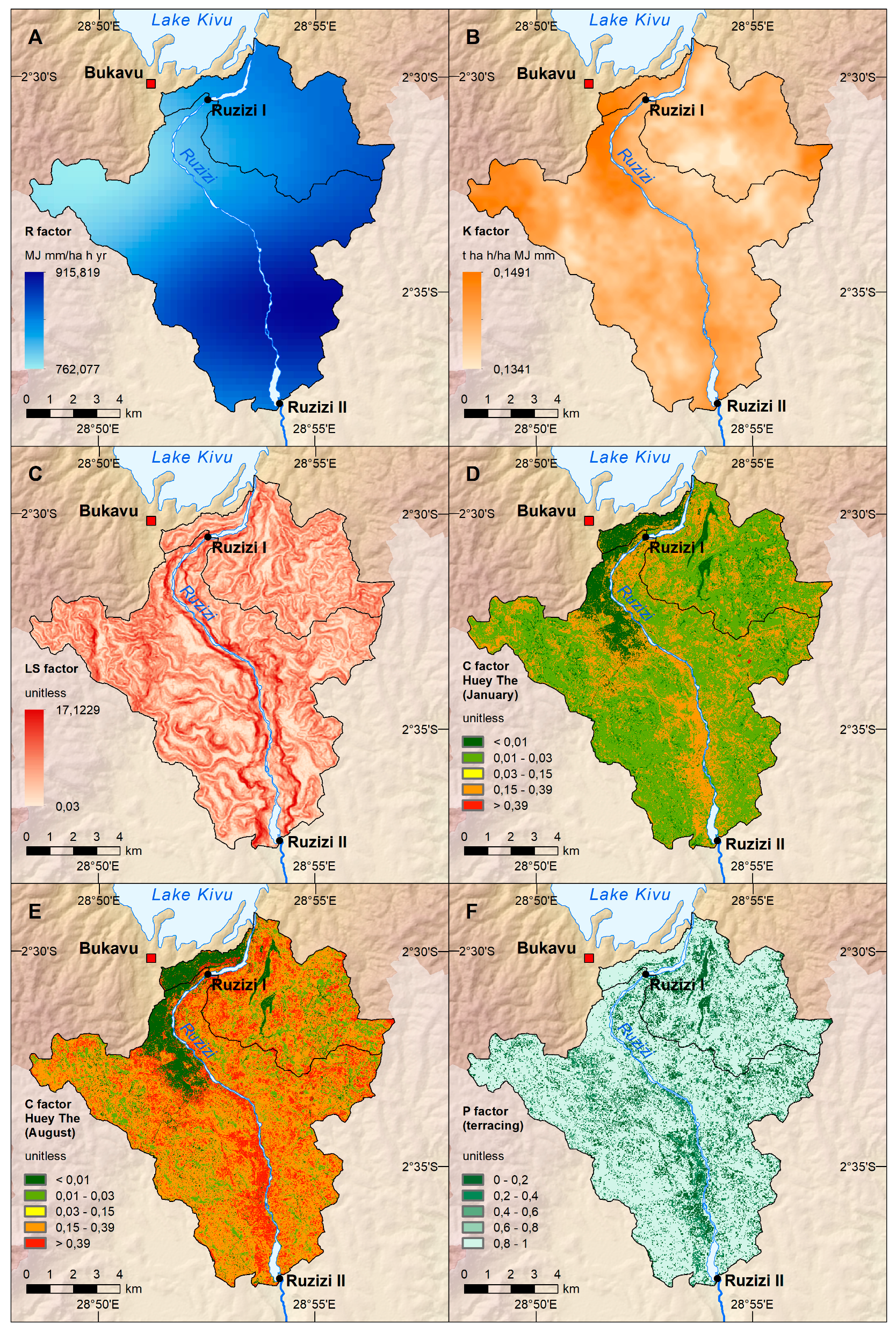
The R factor calculation in USLE is based on the mean annual rainfall. In (R)USLE the mean monthly rainfall is considered to cover the differences between the rainy and dry seasons (Equation (2); [1]; Figure 2A). For R factor calculation, the CHIRPS data (Climate Hazards Group InfraRed Precipitation with Station data; [45]) was used as it is available in a relatively high spatial resolution (Table 1). Mean monthly and mean annual rainfall was calculated from daily data of 2016. The unit of the rainfall and runoff factor is MJ · mm · ha−1 · h−1 · yr−1.
where pi is the mean monthly rainfall (mm) and p is the mean annual rainfall (mm).
The K factor reflects the soil erodibility due to different soil types and its texture. The Equations (3)–(7) consider organic carbon and different sizes of soil particles and their susceptibility for erosion, which is dependent on their ability to achive infiltration (Figure 2B). For example, infiltration into sandy soils is high due to their high sand contents and therefore causes large pore sizes (see [3,20] for further examples). The AfSIS dataset (African Soil Information Service; Table 1) contains grain sizes and organic carbon content for different soil depths [16,46,47] and was therefore used for K factor calculations. The unit of the soil erodibility factor is t · ha · h · ha−1 · MJ−1 · mm−1.
where fcsand is the factor of low soil erodibility due to coarse-grained sand particles in the soil; fcl-si is the factor for low soil erodibility due to high clay-silt ratios; forgc is the factor for reduced soil erodibility due to high carbon content; fhisand is the factor for reduced soil erodibility due to very high sand content; ms is the percentage of sand with grain sizes of 0.05–2 mm; msilt is the percentage of silt with grain sizes of 0.002–0.05 mm; mc is the percentage of clay with grain sizes of <0.0002 mm; orgC is the percentage of organic carbon.
The most complex factor is the LS factor representing the topography. The main parts of the LS factor are the slope length factor (L), and the slope steepness factor (S) which both have a distinct effect on erosion of soil material on slopes. The slope length reflects “the distance from the point of origin of overland flow to the point where either the slope gradient decreases enough that deposition begins, or the runoff water enters a well-defined channel” [1]. The soil loss increases as the slope length increases. The L factor is calculated as a ratio to a plot of 22.13 m (72.6 ft) due to field measurements conducted by Wischmeier and Smith [1]. For the S factor, Wischmeier and Smith [1] determined that “soil loss increases much more rapidly than runoff as slopes steepen” (Equations (12) and (13)) (Figure 2C). For LS factor calculations, the SRTM DEM was used. It is actually available as version 3, which consists of a 30 m resolution DEM covering an area between 60° North and 56° South [48]. The active radar system is mostly impervious to atmospheric disturbances due to the long-wave X-ray radiation used to produce the DEM (Table 1). Flow accumulation, slope (in degree and percent [tangent]), and aspect were calculated following the approach of Karamage et al. [16] because it also considers steep angles, which occur frequently in the study area (see Equations (8)–(11)). The LS factor is dimensionless.
where Li.j is the slope length factor with coordinates i.j for one grid cell; Ai.j is the flow accumulation area at the inlet of a grid cell counting the number of cells of the part of the catchment with flow orientation into the respective grid cell; D is the size of a grid cell (m); the exponent m represents the ratio β of rill erosion, which caused by overland flow to inter-rill erosion caused by the impact of raindrops; θ is the slope angle in degrees; ai.j is the aspect or exposition of the grid cell.
Originally, “the C factor measures the combined effect of all the interrelated cover and management variables” [1], focusing mainly on different landuse or cropping techniques. To also consider landcover like savanna, trees, or even forests, a supervised classification was conducted following the Maximum Likelihood Procedure. It was based on bands 2, 3, 4, and 8 of high resolution Sentinel 2a MSI to meet the requirements of small farms that are less than a hectare [16]. The training areas were selected with band combinations 4-3-2 and 8-4-3 and matched to field observations from August 2016. Ground truthing was done using high resolution images provided by ArcGIS 10.x base maps [33].
Because of the different densities of vegetation cover listed by the Malaysian Department of Agriculture (2010, cited from Huey The [23]) we could also consider burned grasses and bushland during the dry season; the bushland value was adjusted to 100% bush cover for January (0.03) and to a higher value for August, representing an intermediate value between 100% and 50% cover (0.15). Based on the classification results, a C factor value was matched to each class following the detailed list of Huey The [23] (for Malaysia) and our own adjustments according to the seasons (see Table 2, Table 3, Figure 2D,E). The cover and management factor is dimensionless.
The support practice factor P represents the land management practices used to mitigate erosion like contour farming or terracing on steep slopes with farmland, or can be differently expressed to reduce the rate of runoff [2]. To reflect the current situation in the study area, a P factor of 1.00 was assumed according to the suggestions of Reusing et al. [25], reflecting no management activities (Figure 3A). As terracing can already be observed at selected slopes on the Rwandan side of Ruzizi valley, the respective P factor values were assigned in a further step representing sensible land management techniques to reduce the future soil loss (Table 4; Figure 2F and Figure 3B). For the allocation of P factor values to the study area, the results of the supervised classification and the slope dataset were used in accordance to the P factor list of Shin [49] (Table 4). The support practice factor is dimensionless.
Before data implementation, all datasets (Table 1) were clipped by the outline of the study area and reprojected to Universal Transverse Mercator (UTM), zone 35 South.
3. Results
The value of the R factor is the highest within the (R)USLE model ranging between 762 and 916 MJ mm/ha h yr (Equation (2), Table 5, Figure 2A). The logarithmic term changes the areal distribution of R factor in comparison to the precipitation pattern, with slightly higher rates in the southern part of the study area and lower rates in the eastern part. The K factor calculated for the study area ranges between 0.13 and 0.15. In the areas surrounding Bukavu, there is a high K factor value (Figure 2B) that is mainly triggered by low clay and organic carbon content while the amount of high sand () content also leads to a higher K factor. Obviously, the low clay content prevails, or conversely high clay content leads to less erosion and to a lower K factor. Further west and in the extreme east, there is also a high K factor value with medium clay content but high silt content (Figure 2B, Table 5, Equations (3)–(7)).
The L factor and flow accumulation show nearly the same spatial pattern, highlighting the main input into L factor calculation. Low values for slope length are occurring at the steep but short slopes on both sides of Ruzizi River. The L factor has a lower range and lower values in contrast to the S factor: the L factor varies between 1 and 2.3, while the S factor varies between 0 and 13.4 (Table 5, see Figure 2C for LS factor).
The assignment of C factor values from Huey The [23] to the different land cover classes lead finally to min and max C factors of 0 (for water areas) and 1 (for pits, Table 3) for both the January and August calculations. Slightly different values considering rainy and dry season with the respective growth state of the vegetation lead to mean values of 0.27 and 0.28, respectively. The maps highlight the most affected areas along the central Ruzizi valley, mainly consisting of crop land, but also some grasses and bushes (Table 5, Figure 2D,E). Only a small number of forest residuals lead to small C values. The high resolution satellite images from the Sentinel 2a MSI sensor displays the small parcels of the mostly small-holder farmers in the region as observed during field work. Also, C factor values (Figure 2D,E) and (R)USLE results (Figure 3) reflect this kind of land use.
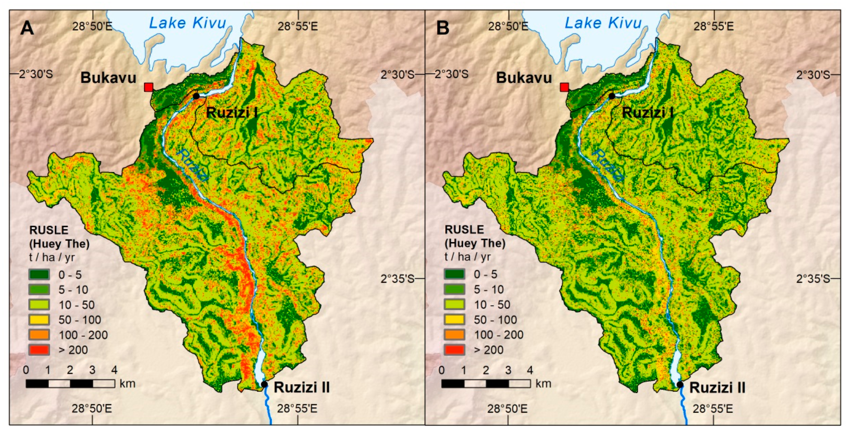
Looking at the spatial pattern of (R)USLE results, it is obvious that the highest soil loss values occur mainly in the central southern part of the study area linked to the broad extend of agricultural area at the steep slopes of the deep incised Ruzizi River (Figure 3A). This is different to the situation at the eastern border of the river where there is more heterogeneous land cover and, hence, no such large scale estimated soil loss occurs. The smallest rates of loss can be found along the thalwegs in the valleys. This loss is distinctly linked to the topography and the respective low LS factor values. On Rwandan side in the catchment of Ruzizi I, there are some rice paddies with a small amount of erosion that also follow the floodplain of two tributaries of the Ruzizi River. The (R)USLE values of these areas are characterized again by a combination of both land cover and topography reflected by C and LS factors, respectively. Finally, the area of Bukavu has low values of erosion due to having sealed surfaces (Figure 3A).
The mean value of (R)USLE calculations for catchments Ruzizi I and II is 48 t/ha/yr with a sum of 577,124 t/yr. As precipitation and land cover were gathered in 2016, these calculations can be matched to this year (Table 6). The P factor used for (R)USLE distinctly reduces the results of soil loss calculations, reflecting an improvement of land management practices. Conservation support practices like terracing can be partially observed in the region, mainly on the Rwandan side. If such techniques can be established in the whole area with high slope angles, then soil erosion can be reduced by 41.5%, which is a mean soil loss of 28 t/ha/yr or a total of 337,710 t/yr for both catchments (Table 6; Figure 3B).
The comparison of the catchments shows a slightly higher estimated mean soil loss in Ruzizi II catchment, which is mainly linked to the high rates of crop land at the slope of Ruzizi River in contrast to a more heterogeneous landscape in Ruzizi I catchment that is mainly characterized by less incised tributaries of the Ruzizi River (Figure 2C). Additionally, the amount of crop land is higher in the Ruzizi II catchment (Table 6). However, the reduction of mean soil loss by P factor is nearly the same in both catchments (81.7% in Ruzizi I; 81.3% in Ruzizi II), pointing to a comparable distribution of crop land shares in regard to the slope (Table 6).
For validation reasons the results dataset of Karamage et al. [16] was kindly provided by the first author. Before comparison with our own results, this dataset was clipped with the catchment area of Ruzizi I, and very high and obviously incorrect values for soil loss estimates of around 100.000 t/ha/yr were replaced by the value 1000 (see Max values in Table 7 and Table 8). However, the USLE results from our own calculations exactly following the paper of Karamage et al. [16] led to results distinctly higher for the Ruzizi I sub-catchment.
Therefore, it is advisable to also consider erosion plots for ground validation. There was a field study done by König [50] over several years close to Butare in southern Rwanda less than 100 km east of Bukavu. It was conducted using the framework of PASI (Projet Agricole et Social Interuniversitaire) and co-initiated by Koblenz-Landau University. This site is established on a ferralitic soil with a mean annual precipitation rate of 1280 mm and fits well to the study area near Bukavu, respectively. An erosion plot was characterized by bare soil and another by traditional farming of different cultures, both on a slope of 28% with mean annual soil loss rates of >400 and 120–250 t/ha/yr, respectively. Comparing the results of soil loss estimations with König’s [50], the results of RUSLE model following the C factor of Huey The [23] and the R factor of Prasannakumar et al. [15] fit best, as well as when considering the maximum value of soil loss, which is 361 t/ha/yr. The dataset of Karamage et al. [16] has an output of 24.68 t/ha/yr for the slope gradient of 25%–30% (Table 8).
Finally, a regional proxy can be used for validation. Muvundja et al. [51] gathered turbidity data from September 2016 to October 2017 at the site of Ruzizi II. They transferred the measurements via a linear model to total suspended solids (TSS) of 12.9 t/ha/yr at this location. For Ruzizi II, an area normalized value of 50.58 t/ha/yr can be calculated based on (R)USLE results (Table 6, Ruzizi II) which is four times higher than TSS; hence, it is reasonable when considering the deposition on the slopes, along the river bank, and in the river bed during transport [1,52]. Eisenberg and Muvundja [53] also tried to estimate turbidity based on the Normalized Difference Turbidity Index (NDTI). When comparing Ruzizi I and II catchments, it becomes obvious that Ruzizi I has lower mean estimated soil loss than Ruzizi II. This observation was also confirmed by NDTI measurements of Ruzizi I and II dam reservoirs, the latter being the most turbid. Overall, the results of the soil loss model matched well to NDTI and turbidity measurements in the study area, while also hinting towards the potential source area of most of the sediments [51,53].
4. Discussion
Due to a high range of C and LS values, these factors led to high (R)USLE results, as R and K factors are characterized by only slight differences in the study area (Table 5, Figure 2 and Figure 3A). However, e.g., high sand content leads to a low K factor and therefore to reduced erosion as the infiltration is high due to the high void space (c.f. [20]). It can also be observed that silt content is responsible for higher K factor values leading to higher erosion. Higher content of organic carbon usually leads to reduced susceptibility to erosion; hence, it also shows its peak in the western region because it has a lower weight in K factor calculations than silt content.
Regarding LS and C factors, the steep slopes along Ruzizi valley covered by crop and grass land heavily contribute to high rates of soil loss. A more detailed look on the spatial pattern along the valley highlights the highest soil loss rates on the DRC’s part of the study area. It is assumed that the people of neighboring Bukavu use the land intensively by conducting grazing and cropping activities due to LULC classification based on high resolution satellite images and personal observations in the field. The next town on Rwandan side is Kamembe/Cyangugu (Ruzizi District), which is situated north of the sub-catchments. During field work several terraces could be observed on the Rwandan border, hinting at improved land management practices in that region limiting soil loss. Even if these shallow sections are not visible in the DEM due to their small sizes in comparison to the spatial resolution of the DEM (Table 1), they contribute to lower (R)USLE results: Along the steps between the terraces trees and bushes are growing which protect against erosion. In the classification process for C factor calculation, these areas were mainly classified as bushland with a distinct lower value as crop land (Table 3) and therefore had a lower (R)USLE value. This way of processing probably led to proper results; hence, when adding the P factor, bushland will not be considered. Karamage et al. [16] suggested using data of high spatial resolution to consider the heterogeneous land use in the study area, but even the Sentinel 2a MSI data (Table 1) cannot always delineate the small parcels.
Considering erosion plots and turbidity measurements the (R)USLE results fit fine reflecting a high rate of soil loss in the study area mainly linked to crop land along the steep slopes of Ruzizi River. The validation following Karamage et al. [16] did not match. Their results seem to be correct; however, their R factor was originally used for soil loss modeling in Hawaii [54] with roughly the half of the mean annual precipitation compared to Bukavu. When modifying their R factor equation following Prasannakumar et al. [15] the results of soil loss estimations fitted better, even if C factors were based on NDVI or on predefined values for different land cover classes [33], (Table 2); hence, it seems that it is not a problem with R factor but with K factor calculations. Karamage et al. [16] listed K factors from 0.009–0.11 in the table of contents of the respective figure with only small areas with the highest value and broad areas with values from 0.009–0.01 t ha h/ha MJ mm. They also listed several soils like Acrisols, Andosols, and Ferralsols covering the Lake Kivu region. The K factor calculated for Ruzizi I and II sub-catchments following the terms used by Karamage et al. [16] are partially higher by the factor 10 in a regional soil environment, which is comparable to the surroundings of Lake Kivu. According to tables of Ahmad Ali and Hagos [18], Bewket and Teferi [17], or Hurni [21], the brown to red soils can be matched to K factor values of 0.15–0.25. Due to their small K factor, perhaps the incongruous R factor term from Lo et al. [54] was selected to increase the results to fit the assumptions better (Table 7).
However, even if the validation matches the results, (R)USLE calculates only the soil loss in the respective scale of the input data. It is an approximation. E.g., along Ruzizi I reservoir some gullies were identified in the field linked to sewage channels from near Bukavu. USLE was originally developed for sheet and rill erosion, not for considering deeply incised linear features like gullies [1]. Additionally, as Ruzizi River is following a tectonically active region, landslides also occur regularly, adding huge amounts of sediments to the system [35,55]. These processes do not happen periodically, so it is difficult to add a distinct amount of sediment input to the model.
To reduce soil loss rates, the P factor was introduced to (R)USLE considering contouring, strip-cropping, and terracing as land management techniques. For the steepest topography along Ruzizi valley, terracing is mainly suggested. However, as the study area is situated in naturally occurring montane forest zone management techniques like agro-forestry should also be introduced to the people. König [50] tested such systems on PASI erosion plots in Rwanda, leading to a distinct reduction of soil loss. These systems could use a respective C factor for forest instead of cropland (Tabs. 2, 3). During field work, reforestation activities could already be observed in the central southern part of the study area along the reservoir of Ruzizi II to improve the protection against erosion. However, these activities are in conflict with current land use practices of the local population. Agro-forestry needs to be established in a sustainable and appropriate manner to the riparian population, though it must be used by the dam operators to combat reservoir siltation and water quality degradation.
5. Conclusions
The (Revised) Universal Soil Loss Equation is a powerful tool used to estimate soil loss in a semi-automated way. There is a wide range of modifications for factor calculations and it seems a bit like a toolbox in which the single terms can be modified as long as the best results will be received. Therefore, a form of validation using field measurements is necessary. This paper identified the (R)USLE model based on R factor equations from Prasannakumar et al. [15] and a C factor list offered by the Malaysian Department of Agriculture (2010; cited after Huey The [23]) to fit best to the erosion plots established by König [50] and turbidity and NDTI measurements in the study area [51,53]. According to this model, a total soil loss of 577,124 t/yr can be estimated for the study area (Table 6). The highest rates occur on the steep slopes of Ruzizi valley along the crop and grass land. Due to C factor calculations based on high resolution Sentinel 2a images, the heterogeneous LULC pattern is reflected by (R)USLE results.As a result, differences between land use practices in Rwanda and the DRC became obvious. This approach could also be used to monitor re-forestation activities at the slopes of Ruzizi II reservoir and its influence on soil loss. We recommend adjusting (R)USLE models for comparable regions which are characterized by such small scale farming, including most sub-Saharan countries.
It became clear that errors occur in USLE model calculation; however, they cannot always be identified when only reviewing the papers carefully. Instead, the models have to be re-calculated. The results show the most vulnerable areas along the steep slopes with sparse vegetation or intensive agriculture without an adequate land management practice (see Figure 3). To adjust the model, high resolution DEMs could help to identify small-scale topographic variations like terraces. Unfortunately, e.g., LIDAR (LIght Detection and Ranging) data is not freely available for developing countries which need such soil loss estimations urgently. A time intensive acquisition of areas with terraces or strip-cropping with freely available high resolution satellite images could be an alternative.
Author Contributions
Conceptualization, J.E. and F.A.M.; methodology, J.E.; software, J.E.; validation, J.E. and F.A.M.; formal analysis, J.E.; investigation, J.E.; writing—original draft preparation, J.E.; writing—review and editing, J.E. and F.A.M.; visualization, J.E.; project administration, F.A.M.; funding acquisition, F.A.M. All authors have read and agreed to the published version of the manuscript.
Funding
This research was funded by the Volkswagen Foundation, grant number #89358 (Knowledge for Tomorrow).
Acknowledgments
We would like to thank Fidele Karamage and his co-authors for providing their results [16] as a raster dataset for exact comparison of the results, and Fredie Kern from the University of Applied Sciences in Mainz for supervising the model which this paper refers to. We also thank all other project members from the Unité d’Enseignement et de Recherche en Hydrobiologie Appliquée (UERHA), ISP Bukavu, for their field assistance during the ground truthing and the reviewers for their important remarks.
Conflicts of Interest
The authors declare no conflict of interest.
Appendix A

Table A1.
Overview of R factor calculations of selected publications.
| Author(s), Region, Formula | Model | Factor |
|---|---|---|
| [17], Chemoga WS, Ethiopia and [18], Awassa, Central Ethiopia | USLE | Rainfall erosivity (R) |
| R = −8.12 + (0.562 × P) | (2) | |
| [19], Kulhan, India | USLE | Rainfall erosivity (R) |
| R = P × 0.5 | (3) | |
| [16], Kivu, DRC and Rwanda | USLE | Rainfall-runoff erosivity (R) |
| R = 38.46 + 3.48 × P | (4) | |
R is the rainfall erosivity factor (MJ mm ha−1h−1 per year); P is the mean annual rainfall (mm).
Beneath complex calculations, also lists are used containing different soil colors and their respective K factor as the soil color is directly linked to its texture. Hurni [21] and Bewket and Teferi [17] are matching K factor 0.15, 0.2, 0.25 and 0.3 to black, brown, red and yellow soils, respectively.
Table A2.
Overview of K factor calculations of selected publications.
| Author(s), Region, Formula | Model | Factor |
|---|---|---|
| [20], Nethravathi, Southwest India ** | RUSLE | Soil erodibility (K) |
| K = 27.66 × m1.14 × 10−8 × (12 − a) + 0.0043 × (b − 2) + 0.0033 × (c − 3) | (7) | |
| (7a) | ||
* fcsand is the factor of low soil erodibility due to coarse-grained sand particles in the soil; fcl-si is factor for low soil erodibility due to high clay-silt ratios; forgc is the factor for reduced soil erodibility due to high carbon content; fhisand is the factor for reduced soil erodibility due to very high sand content; ms is the percentage of sand with grain sizes of 0.05–2 mm; msilt is the percentage of silt with grain sizes of 0.002–0.05 mm; mc is the percentage of clay with grain sizes of <0.0002 mm; orgC is the percentage of organic carbon. ** a is organic matter in %; b is a structure code in which (1) is very structured or particulate, (2) is fairly structured, (3) is slightly structured, and (4) is solid; c is the profile permeability code in which (1) is rapid, (2) is moderate to rapid, (3) is moderate, (4) is moderate to slow, (5) is slow, and (6) very slow.
Table A3.
Overview of LS factor calculations of selected publications.
| Author(s), Region, Formula | Model | Factor |
|---|---|---|
| [16], Kivu, DRC and Rwanda * | USLE | Slope Length and Steepness Factor (LS) |
| (8) | ||
| (8a) | ||
| (8b) | ||
| (8c) | ||
| (9a) | ||
| (9b) | ||
| [17], Blue Nile Basin, Ethiopia ** | USLE | Topographic factor (LS) |
| (10) | ||
| [20], Nethravathi, Southwest India | RUSLE | Topographic factor (LS) |
| (11) | ||
| [2], Palouse, Idaho, US *** | RUSLE | Topographic factor (LS) |
| s < 9% | (12a) | |
| s > 9% | (12b) | |
* Karamage et al. [16] modified the original equation according to Desmet and Govers [26] to consider also the upstream contribution area for complex slopes where Li.j is the slope length factor with coordinates i.j for one grid cell; Ai.j is the flow accumulation area at the inlet of a grid cell counting the number of cells of the part of the catchment with flow orientation into the respective grid cell; D is the size of a grid cell (m); the exponent m represents the ratio β of rill erosion which caused by overland flow to inter-rill erosion caused by the impact of raindrops; θ is the slope angle in degrees; ai.j is the aspect or exposition of the grid cell. Karamage et al. [16] were using the formula of slope steepness factor based on McCool et al. [27] who differentiate between slope angles of less and more than 9% to consider also steep angles in their study area along the East African Rift. ** λ is the distance between onset of runoff and the receiving channel; m is an exponent depending on the slope steepness, this factor will not be calculated as by Karamage et al. [16] but assigned due to slope angle in percent (0 to 5% will be assigned with values of 0.2 to 0.5) which is according to Wischmeier and Smith [1]; x is the slope angle in percentage. *** Qa is the flow accumulation grid with the grid size M; y is an exponent depending on the slope angle (see explanation above for exponent m); Sg is the slope angle in percentage.
References
- Wischmeier, W.H.; Smith, D.D. Predicting Rainfall Erosion Losses: A Guide to Conservation Planning; Agriculture Handbook: Washington, DC, USA, 1978; Volume 537, 58p. [Google Scholar]
- Renard, K.G.; Foster, G.R.; Weesies, G.A.; McCool, D.K.; Yoder, D.C. Pre-dicting Soil Erosion by Water: A Guide to Conservation Planning with the Revised Universal Soil Loss Equation (RUSLE); Agriculture Handbook: Washington, DC, USA, 1997; Volume 703, 384p. [Google Scholar]
- Benavidez, R.; Jackson, B.; Maxwell, D.; Norton, K. A review of the (Revised) Universal Soil Loss Equation ((R)USLE): With a view to increasing its global applicability and improving soil loss estimates. Hydrol. Earth Syst. Sci. 2018, 22, 6059–6086. [Google Scholar] [CrossRef] [Green Version]
- Church, M.; Moo, M.-K. Geography of surface runoff: Some lessons for research. In Processes in Hillslope Hydrology; Anderson, M.G., Burt, T., Eds.; John Wiley and Sons: Chichester, UK, 1990; pp. 299–325. [Google Scholar]
- Ambassa-Kiki, R.; Nill, D. Effects of different land management techniques on selected topsoil properties of a forest Ferralsol. Soil Tillage Res. 1999, 52, 259–264. [Google Scholar] [CrossRef]
- Labrière, N.; Locatelli, B.; Laumonier, Y.; Freycon, V.; Bernoux, M. Soil erosion in the humid tropics: A systematic quantitative review. Agric. Ecosyst. Environ. 2015, 203, 127–139. [Google Scholar] [CrossRef]
- Morgan, R.P.C.; Quinton, J.N. Erosion Modeling. In Landscape Erosion and Evolution Modeling; Harmon, R.S., Doe, W.W., III, Eds.; Kluwer Academic/Plenum Publishers: New York, NY, USA, 2001; pp. 117–143. [Google Scholar]
- Wu, T.H.; Hall, J.A.; Bonta, J.V. Evaluation of Runoff and Erosion Models. J. Irrig. Drain. E-asce. 1993, 119, 364–381. [Google Scholar] [CrossRef]
- Reyes, M.R.; Cecil, K.D.; Raczowski, C.W.; Gayle, G.A.; Reddy, G.B. Comparing GLEAMS, RUSLE, EPIC and WEPP Soil Loss Prediction with Observed Data from Different Tillage System. In Proceedings of the 10th International Conference on Soil Conservation (ISCO), West Lafayette, IN, USA, 23–28 May 1999. [Google Scholar]
- Chandramohan, T.; Venkatesh, B.; Balchand, A.N. Evaluation of three soil erosion models for small watersheds: International Conference on water resources, coastal and ocean engineering (ICWRCOE 2015). Aquat. Procedia 2015, 4, 1227–1234. [Google Scholar] [CrossRef]
- Hrissanthou, V. Estimate of sediment yield in a basin without sediment data. Catena 2005, 64, 333–347. [Google Scholar] [CrossRef]
- ARS. Watershed Physical Processes Research. 2016. Available online: https://www.ars.usda.gov/southeast-area/oxford-ms/national-sedimentation-laboratory/watershed-physical-processes-research/docs/revised-universal-soil-loss-equation-rusle-welcome-to-rusle-1-and-rusle-2/ (accessed on 15 April 2020).
- Sundara Kumar, P.; Praveen, T.V.; Prasad, A. Simulation of sediment yield over un-gauged stations using MUSLE and Fuzzy Model. Aquat. Procedia 2015, 4, 1291–1298. [Google Scholar] [CrossRef]
- Sotiropoulou, A.-M.; Alexandridis, T.; Bilas, G.; Karapetsas, N.; Tzellou, A.; Silleoa, N.; Misopolinos, N. A user friendly GIS model for the estimation of erosion risk in agricultural land using the USLE. In Proceedings of the International Conference on Information and Communication Technologies for Sustainable Agri-Production and Environment, Skiathos, Greece, 8–11 September 2011. [Google Scholar]
- Prasannakumar, V.; Vijith, H.; Abinod, S.; Geetha, N. Estimation of soil erosion risk within a small mountainous sub-watershed in Kerala, India, using Revised Universal Soil Loss Equation (RUSLE) and geo-information technology. Geosci. Front. 2012, 3, 209–215. [Google Scholar] [CrossRef] [Green Version]
- Karamage, F.; Shao, H.; Chen, X.; Ndayisaba, F.; Nahayo, L.; Kayiranga, A.; Omifolaji, J.K.; Liu, T.; Zhang, C. Deforestation effects on soil erosion in the lake Kivu basin, D.R. Congo-Rwanda. Forests 2016, 7, 281. [Google Scholar] [CrossRef] [Green Version]
- Bewket, W.; Teferi, E. Assessment of soil erosion hazard and prioritization for treatment at the watershed level: Case study in the Chemoga watershed, Blue Nile basin, Ethiopia: Case study in the Chemoga watershed, Blue Nile Ba-sin, Ethiopia. Land Degrad. Dev. 2009, 20, 609–622. [Google Scholar] [CrossRef]
- Ahmad Ali, S.; Hagos, H. Estimation of soil erosion using USLE and GIS in Awassa Catchment, Rift valley, Central Ethiopia. Geoderma Reg. 2016, 7, 159–166. [Google Scholar]
- Devatha, C.P.; Vaibhav, D.; Renukaprasad, M.S. Estimation of Soil loss using USLE model for Kulhan Watershed, Chattisgarh—A case study. Aquat. Procedia 2015, 4, 1429–1436. [Google Scholar] [CrossRef]
- Ganasri, B.P.; Ramesh, H. Assessment of soil erosion by RUSLE model using remote sensing and GIS—A case study of Nethravathi Basin. Geosci. Front. 2016, 7, 953–961. [Google Scholar] [CrossRef] [Green Version]
- Hurni, H. Erosion–Productivity–Conservation Systems in Ethiopia. Proceedings IV International Conference on Soil Conservation: Soil Conservation and Productivity, Maracay, Venezuela, 3–9 September 1985. [Google Scholar]
- Knijff, v.d.J.M.; Jones, R.J.A.; Montanarella, L. Soil Erosion Risk Assessment in Europe. Ispra, Italy. 2000. Available online: https://www.unisdr.org/files/1581_ereurnew2.pdf (accessed on 22 April 2020).
- Teh, S.H. Soil Erosion Modeling Using RUSLE and GIS on Cameron Highlands, Malaysia for Hydropower Development. Master Thesis, University of Iceland, Reykjavik, Iceland, 21 March 2011. [Google Scholar]
- Eweg, H.P.A.; van Lammeren, R. The Application of Geographic Information System at the Rehabilitation of Degraded and Degrading Areas of Tigray, Ethiopia; Agricultural University: Wageningen, The Netherlands, 1996; p. 79. [Google Scholar]
- Reusing, M.; Schneider, T.; Ammer, U. Modelling soil loss rates in the Ethiopian Highlands by integration of high resolution MOMS-02/D2-stereo-data in a GIS. Int. J. Remote Sens. 2000, 21, 1885–1896. [Google Scholar] [CrossRef]
- Desmet, P.; Govers, G. A GIS procedure for automatically calculating the USLE LS factor on topographically complex landscape units. J. Soil Water Conserv. 1996, 51, 427–433. [Google Scholar]
- McCool, D.; Brown, L.; Foster, G.; Mutchler, C.; Meyer, L. Revised slope steepness factor for the universal soil loss equation. Trans. ASAE 1987, 30, 1378–1396. [Google Scholar] [CrossRef]
- Mbiya, K. Le problème de l’éosion anthropogique à Bukavu. In L’Homme Responsable et Victime du Problème—Une Restauration Problématique; Mémoire de Géographie: Bukavu, Congo-Kinshasa, 1980. [Google Scholar]
- Birindwa, C.R. Dynamique Sédimentaire Dans le Bassin Versant de la Rivière Wesha, Ville de Bukavu. Mémoire Effectué Dans le Cadre de la Formation en Géorisques, ISP Bukavu. 2015. Available online: https://www.semanticscholar.org/paper/DYNAMIC-SEDIMENTARY-IN-WATERSHED-OF-WESHA-RIVER%2C-Cubwe/d0c8d00cca335565e0cb2d58412a79402b790c66 (accessed on 14 April 2020).
- Dyson, M.; Bergkamp, G.; Scanlon, J. (Eds.) Flow. The Essentials of Environmental Flows; IUCN: Gland, Switzerland; Cambridge, UK, 2003. [Google Scholar]
- King, J.; Brown, C. Environmental Flows: Striking the balance betwenn development and resource protection. Ecol. Soc. 2006, 11, 26. [Google Scholar] [CrossRef] [Green Version]
- King, J.; Brown, C. Integrated basin flow assessments: Concepts and method development in Africa and South-East Asia. Freshw. Biol. 2009, 55, 127–146. [Google Scholar] [CrossRef]
- Eisenberg, J. Multi-Temporal Quantification of Erosion in Selected Catchment Areas of the Ruzizi River (DRC) Using the (R)USLE Model in ArcGIS ModelBuilder (10.5). Master Thesis, University of Applied Science Mainz, Mainz, Alemanha, 2018. [Google Scholar]
- Cazenave-Piarrot, A.; Sabushimike, J.-M. Les paysages: Des lacs et des mon-tagnes. Chapitre Une nature soumise à de nombreuses contraintes. In Atlas des Pays du Nord-Tanganyika; Cazenave-Piarrot, A., Ndayirukiye, S., Valton, C., Eds.; Institut de Recherche Pour le Développement (IRD): Marseille, France, 2015; pp. 20–23. [Google Scholar]
- Nobile, A.; Dille, A.; Monsieurs, E.; Basimike, J.; Bibentyo, T.M.; d’Oreye, N.; Kervyn, F.; Dewitte, O. Multi-Temporal DInSAR to Characterise Landslide Ground Deformations in a Tropical Urban Environment: Focus on Bukavu (DR Congo). Remote Sens. 2018, 10, 626. [Google Scholar] [CrossRef] [Green Version]
- Nahimana, L. Les dispositifs géologiques et les sols. Chapitre: Une nature soumise à de nombreuses contraintes. In Atlas des Pays du Nord-Tanganyika; Cazenave-Piarrot, A., Ndayirukiye, S., Valton, C., Eds.; Institut de Recherché Pour le Développement: Marseille, France, 2015; pp. 32–37. [Google Scholar]
- Anne, C.A.T.; Runge, J.; Kampmann, D. Soils of West Africa: Agronomic constraints and degradation. Biodivers. Atlas West Africa 2010, 2, 56–63. [Google Scholar]
- Ndayirukiye, S.; Sabushimike, J.-M. Les climats et les mécanismes climatiques. In Atlas des Pays du Nord-Tanganyika; Cazenave-Piarrot, A., Ndayirukiye, S., Valton, C., Eds.; Institut de Recherché Pour le Développement: Marseille, France, 2015; pp. 28–31. [Google Scholar]
- Runge, J. Landschaftsgenese und Paläoklima in Zentralafrika: Physiogeographische Untersuchungen zur Landschaftsentwicklung und klimagesteuerten quartären Vegetations- und Geomorphodynamik in Kongo/Zaire (Kivu, Kasai, Oberkongo) und der Zentralafrikanischen Republik (Mbomou). In Relief, Boden, Paläoklima; Gebr. Borntraeger: Stuttgart, Germany, 2001; pp. 1–194. [Google Scholar]
- Karhagomba, I.B. La couverture végétale: Une nature soumise à de nombreuses contraintes. In Atlas des Pays du Nord-Tanganyika; Cazenave-Piarrot, A., Ndayirukiye, S., Valton, C., Eds.; Institut de Recherché Pour le Développement: Marseille, France, 2015; pp. 38–41. [Google Scholar]
- Hansen, M.C.; Potapov, P.V.; Moore, R.; Hancher, M.; Turubanova, S.A.; Tyukavina, A.; Thau, D.; Stehman, S.V.; Goetz, S.J.; Loveland, T.R.; et al. High-Resolution Global Maps of 21st-Century Forest Cover Change. Science 2013, 342, 850–853. [Google Scholar] [CrossRef] [PubMed] [Green Version]
- Hansen, M.C.; Stehman, S.V.; Potapov, P.V. Quantification of global gross forest cover loss. Proc. Natl. Acad. Sci. USA 2010, 107, 8650–8655. [Google Scholar] [CrossRef] [Green Version]
- Neuhaus, L. Zugang zu Medizinischer Versorgung in Bukavu, DR Kongo: Eine Netzwerkbasierte GIS-Analyse zur Gesundheitsversorgung. Bachelor’s Thesis, Beuth Hochschule für Technik, Berlin, Germany, 2014. [Google Scholar]
- EGL. Ruzizi III Hydropower Project: Project Structuring and Promotion to Obtain Financing. 2012. Available online: http://addisababa.mfa.ir/uploads/Ruzizi_III_v3_19963.pdf (accessed on 14 April 2020).
- Funk, C.; Peterson, P.; Landsfeld, M.; Pedreros, D.; Verdin, J.; Shukla, S.; Husak, G.; Rowland, J.; Harrison, L.; Hoell, A.; et al. The climate hazards infrared precipitation with stations--a new environmental record for monitoring extremes. Sci. data 2015, 2, 150066. [Google Scholar] [CrossRef] [Green Version]
- Hengl, T.; Heuvelink, G.B.M.; Kempen, B.; Leenaars, J.G.B.; Walsh, M.G.; Shepherd, K.D.; Sila, A.; MacMillan, R.A.; Mendes de Jesus, J.; Tamene, L.; et al. Mapping Soil Properties of Africa at 250 m Resolution: Random Forests Significantly Improve Current Predictions. PLoS ONE 2015, 10, e0125814. [Google Scholar] [CrossRef]
- Hengl, T.; Mendes de Jesus, J.; Heuvelink, G.B.M.; Ruiperez Gonzalez, M.; Kilibarda, M.; Blagotić, A.; Shangguan, W.; Wright, M.N.; Geng, X.; Bauer-Marschallinger, B.; et al. SoilGrids250m: Global gridded soil information based on machine learning. PLoS ONE 2017, 12, e0169748. [Google Scholar] [CrossRef] [PubMed] [Green Version]
- Jarvis, A.; Reuter, H.I.; Nelson, A.; Guevara, E. Hole-filled SRTM for the globe Version 3, the CGIAR-CSI SRTM 30m Database. 2008. Available online: http://srtm.csi.cgiar.org (accessed on 15 April 2020).
- Shin, G. The Analysis of Soil Erosion Analysis in Watersheds Using GIS. Ph.D. Thesis, Gang-Won National University, Chuncheon, Korea, 1999. [Google Scholar]
- König, D. Contribution de l’agroforesterie à la conservation de la fertilité des sols et à la lutte contre le réchauffement climatique au Rwanda. In Proceedings of the Actes des JSIRAUF, Hanoi, Vietnam, 6–9 November 2007; pp. 1–6. [Google Scholar]
- Muvundja, F.A.; Riziki, W.; Dusabe, C.; Alunga, G.; Kankonda, B.A.; Albrecht, C.; Eisenberg, J. Ruzizi River: Environmental flow requirements for Hydropower dams and sediment transport dynamics (Lake Kivu outflow, African Great Lakes Region). J. Inland Waters Submitt. submitted.
- Trimble, S.W. Catchment sediment budgets and change. In Changing River Channels; Gurnell, A., Petts, G., Eds.; Wiley: Chichester, UK, 1995; pp. 201–215. [Google Scholar]
- Eisenberg, J.; Muvundja, F.A. Normalized Difference Turbidity Index (NDTI) for turbidity analyses in the reservoirs of two dammed tropical rivers, Eastern Democratic Republic of the Congo. Zentralblatt für Geologie und Paläontologie. submitted.
- Lo, A.; El-Swaify, S.A.; Dangler, E.W.; Shinshiro, L. Effectiveness of El30 as an erosivity index in Hawaii. In Soil Erosion and Conservation; El-Swaify, S.A., Moldenhauer, W.C., Lo, A., Eds.; Soil Conservation Society of America: Ankeny, IA, USA, 1985. [Google Scholar]
- Moeyersons, J.; Tréfois, P.H.; Lavreau, J.; Alimasi, D.; Badriyo, I.; Mitima, B.; Mundala, M.; Munganga, D.O.; Nahimana, L. A geomorphological assessment of landslide origin at Bukavu, Democratic Republic of the Congo. Eng. Geol. 2004, 72, 73–87. [Google Scholar] [CrossRef]
Figure 1.
Location of the study area on the African continent (A), in Eastern Africa (B), and in the Ruzizi catchment area in the Eastern DRC near Bukavu at Lake Kivu (C).
Figure 1.
Location of the study area on the African continent (A), in Eastern Africa (B), and in the Ruzizi catchment area in the Eastern DRC near Bukavu at Lake Kivu (C).
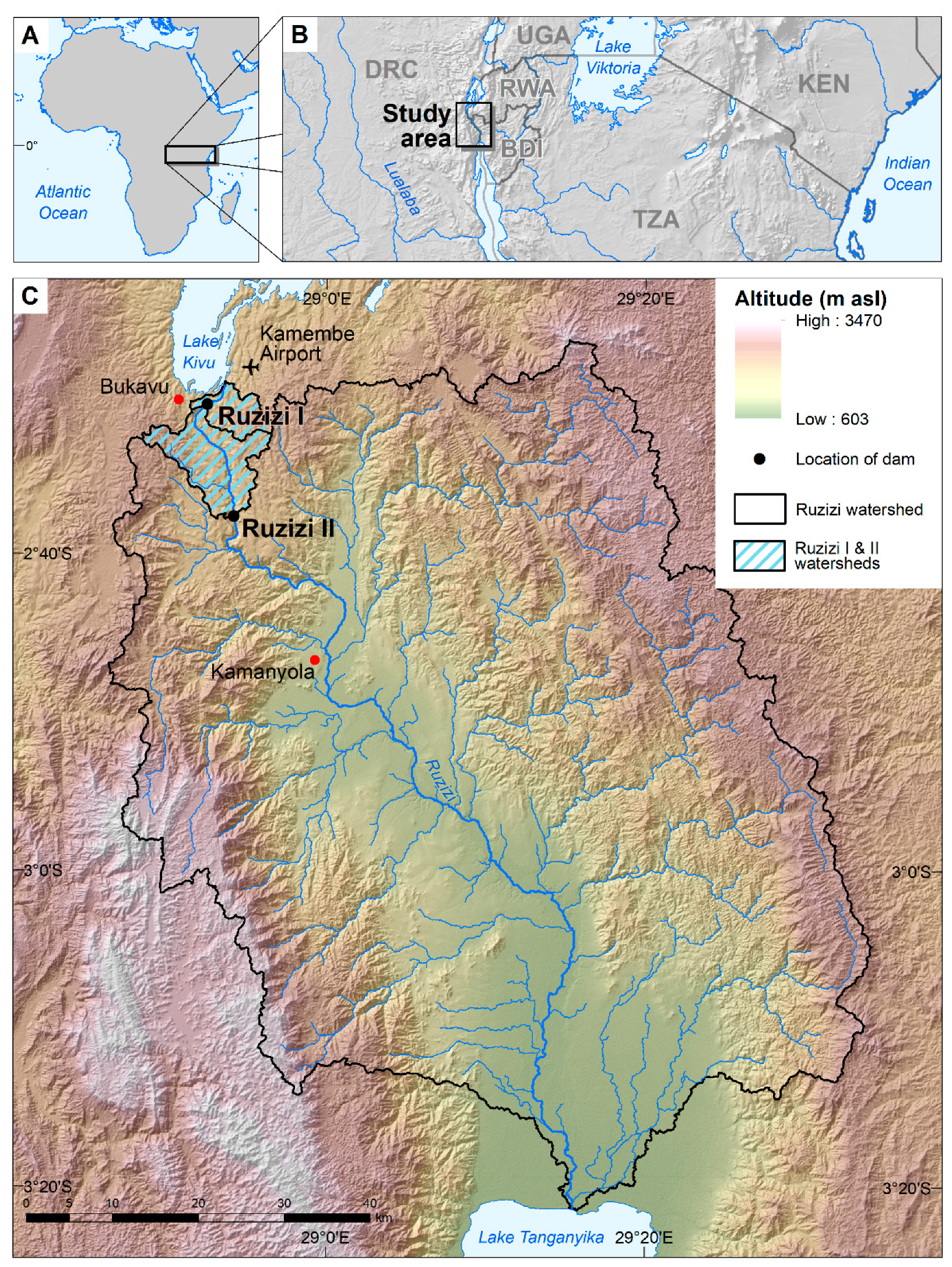
Figure 2.
Resulting maps of the single factors for RUSLE calculations; (A) mean R factor calculated after Prasannakumar et al. [15]; (B) K factor calculated after Karamage et al. [16]; (C) LS factor calculated after Karamage et al. [16]; C factor calculated using the definitions of Malaysian Department of Agriculture (2010, cited from [23]) for rainy (D) and dry seasons (E); (F) P factor [49].

Figure 3.
Results of (R)USLE calculations (A) without and (B) with P factor values for terracing [15,16,23,49].

Table 1.
Freely available datasets to measure (R)USLE factors.
| Factor | Data Set | Provider | Spatial Resolution | Publication Year/Since |
|---|---|---|---|---|
| R | CHIRPS v2.0 (precipitation) | NASA, NOAA | 0.05° (5500 m) | 1981–recent (v2.0) |
| K | AfSIS—Soil Grids (soil) | ISRIC | 250 m | 2017 |
| L and S | SRTMv3 (DEM) | NASA | 1 second (30 m) | 2000, 2015 (v3) |
| C | Sentinel 2a (multispectral: supervised classification is necessary) | ESA | 10 m | Mid–2015–recent |
| P | Results of C calculations to be matched with DEM (see L and S calculations) |
Table 2.
C factor for selected land cover classes in Malaysia [23:41ff] and assigned values used in this study.
Table 2.
C factor for selected land cover classes in Malaysia [23:41ff] and assigned values used in this study.
| Land Cover Type | C Factor [23] | January C Factor | August C Factor |
|---|---|---|---|
| Rangeland | 0.23 | ||
| Forest / tree | |||
| 50% cover | 0.39 | ||
| 100% cover | 0.03 | 0.03 | 0.03 |
| Bushes / scrub | |||
| 50% cover | 0.35 | ||
| 100% cover | 0.03 | 0.03 | 0.15 |
| Grassland 100% cover | 0.03 | 0.03 | 0.30 |
| Mining areas | 1.00 | 1.00 | 1.00 |
| Agricultural crop | 0.38 | 0.38 | 0.40 |
| Paddy (with water) | 0.01 | 0.01 | 0.01 |
| Urbanized areas | |||
| Low density (50% green area) | 0.25 | ||
| Medium density (25% green area) | 0.15 | 0.15 | 0.15 |
| High density (5% green area) | 0.05 | ||
| Impervious (Parking lot, road, etc.) | 0.01 | 0.01 | 0.01 |
Table 3.
Classes of Maximum Likelihood Classification and respective C factors, mainly based on the Malaysian Department of Agriculture (2010 [23:41], see Table 2).
Table 3.
Classes of Maximum Likelihood Classification and respective C factors, mainly based on the Malaysian Department of Agriculture (2010 [23:41], see Table 2).
| Land Cover Class | Remarks | Area of Training Samples (% of 6.49 km²) | Area of Land Cover Class (% of 2300 km²) | C Factor | |
|---|---|---|---|---|---|
| January | August | ||||
| Settlement, road | < 5% Vegetation | 20.60 | 7.82 | 0.01 | 0.01 |
| Village | < 50% Vegetation | 1.34 | 9.04 | 0.15 | 0.15 |
| Pit | 0% Vegetation, mostly artisanal mining | 0.24 | 0.04 | 1.00 | 1.00 |
| Rice field | Mostly represented as areas with dense vegetation in a wetland-like area along flat valleys | 5.73 | 3.14 | 0.01 | 0.01 |
| Crop land | Individual species were not distinguished | 25.74 | 17.71 | 0.38 | 0.40 |
| Grass land | Wide areas, mainly along steep slopes in the hinterland of Ruzizi Valley, burning activities during the dry seasons | 12.83 | 29.98 | 0.03 | 0.30 |
| Bush land | Low trees and bushes (Miombo woodland), natural vegetation in the region, some areas are burned during dry season | 5.94 | 19.22 | 0.03 | 0.15 |
| Forest | Dense forests, mainly as riparian forest along Ruzizi tributaries | 4.75 | 9.96 | 0.03 | 0.03 |
| Water | Mainly Ruzizi River and Lake Kivu | 22.82 | 3.10 | 0.00 | 0.00 |
Table 4.
P factor under different conservation support practices [49].
Table 4.
P factor under different conservation support practices [49].
| Slope (%) | Contouring | Strip-Cropping | Terracing |
|---|---|---|---|
| 0.0–7.0 | 0.55 | 0.27 | 0.10 |
| 7.0–11.3 | 0.60 | 0.30 | 0.12 |
| 11.3–17.6 | 0.80 | 0.40 | 0.16 |
| 17.6–26.8 | 0.90 | 0.45 | 0.18 |
| > 26.8 | 1.00 | 0.50 | 0.20 |
Table 5.
Values of the different (R)USLE factors.
| Factor | Units | Min | Max | Mean |
|---|---|---|---|---|
| R [15] | MJ · mm · ha−1 · h−1 · yr−1 | 762.08 | 915.80 | 845.70 |
| K [16] | t · ha · h · ha−1 · MJ−1 · mm−1 | 0.13 | 0.15 | 0.14 |
| LS [16] | dimensionless | 0.03 | 17.10 | 3.60 |
| L | 0.99 | 2.30 | 1.10 | |
| S | 0.03 | 13.40 | 3.30 | |
| C (rainy season) [23] | dimensionless | 0.00 | 1.00 | 0.27 |
| C (dry season) [23] | dimensionless | 0.00 | 1.00 | 0.28 |
| P (terracing) [16] | dimensionless | 0.10 | 1.00 | 0.48 |
Table 6.
(R)USLE results for different LULC classes and sub-catchments Ruzizi I and II.
| RUSLE | RUSLE with P Factor | |||||||
|---|---|---|---|---|---|---|---|---|
| Catchments | Area | % | Max | Mean | Sum | Max | Mean | Sum |
| (ha) | (t/yr/ha) | (t/yr) | (t/yr/ha) | (t/yr) | ||||
| Ruzizi I | 3,176.92 | 26.38 | 463.62 | 40.50 | 128,654.89 | 431.07 | 24.55 | 77,983.04 |
| Ruzizi II | 8,866.82 | 73.62 | 1,162.23 | 50.58 | 448,469.38 | 1109.95 | 29.29 | 259,726.87 |
| Ruzizi I and II | 12,043.74 | 100.00 | 1,162.23 | 47.92 | 577,124.27 | 1109.95 | 28.04 | 337,709.91 |
| Ruzizi I: LULC | ||||||||
| Settlement, road | 272.11 | 8.57 | 383.70 | 17.54 | 4772.31 | |||
| Village | 218.87 | 6.89 | 423.52 | 67.07 | 14,679.69 | |||
| Pits | 0.48 | 0.01 | 74.33 | 32.44 | 15.45 | |||
| Rice | 184.39 | 5.80 | 229.22 | 6.31 | 1162.78 | |||
| Crops | 602.89 | 18.98 | 463.62 | 102.89 | 62,028.67 | 92.72 | 18.84 | 11,356.82 |
| Grass land | 982.24 | 30.92 | 431.07 | 30.06 | 29,522.31 | |||
| Bush land | 510.88 | 16.08 | 386.29 | 19.63 | 10,026.72 | |||
| Forest | 405.07 | 12.75 | 363.39 | 15.92 | 6446.95 | |||
| Area sum | 3176.92 | 100.00 | 128,654.89 | 77,983.04 | ||||
| Ruzizi II: LULC | ||||||||
| Settlement, road | 546.98 | 6.17 | 714.52 | 27.02 | 14,780.46 | |||
| Village | 697.27 | 7.86 | 792.87 | 73.67 | 51,365.04 | |||
| Pits | 5.33 | 0.06 | 1109.95 | 384.68 | 2051.70 | |||
| Rice | 225.73 | 2.55 | 183.04 | 9.01 | 2033.38 | |||
| Crops | 1875.24 | 21.5 | 1162.23 | 123.92 | 232,381.04 | 232.45 | 23.27 | 43,638.53 |
| Grass land | 2733.66 | 30.83 | 600.82 | 33.27 | 90,956.95 | |||
| Bush land | 2004.77 | 22.61 | 524.92 | 20.34 | 40,782.23 | |||
| Forest | 777.85 | 8.77 | 449.30 | 18.15 | 14,118.57 | |||
| Area sum | 8866.82 | 100.00 | 448,469.38 | 259,726.87 | ||||
Table 7.
(R)USLE results for sub-catchment Ruzizi I.
| Ruzizi I Sub-Catchment (31.76 km²) | Soil Loss in t/ha/yr | t/yr | ||
|---|---|---|---|---|
| Author, Model | Min | Max | Mean | Sum |
| [3], USLE | 0.01 | 1000 | 27.08 | 86,194.81 |
| own calculations following exactly [3], USLE | 0.25 | 3998.20 | 164.52 | 523,695.85 |
| C factor from [2], R factor from [1], RUSLE | 0.00 | 463.62 | 40.50 | 128,654.89 |
Table 8.
(R)USLE results for cropland at a slope of 15–20% and 25–30% in comparison to field work on a slope of 28%.
Table 8.
(R)USLE results for cropland at a slope of 15–20% and 25–30% in comparison to field work on a slope of 28%.
| Author(s), Model | Slope of 15–20% (Soil Loss in t/ha/yr) | Slope of 25–30%(Soil Loss in t/ha/yr) | |||||
|---|---|---|---|---|---|---|---|
| Min | Max | Mean | Min | Max | Mean | ||
| [16], USLE | 0 | 1000 | 21.89 | 0 | 1000 | 24.68 | |
| C factor from [23], R factor from [15], RUSLE | 0 | 275 | 86.85 | 4 | 361 | 136.23 | |
| [43], | bare soil | >400 | |||||
| traditional farming | 120–250 | ||||||
© 2020 by the authors. Licensee MDPI, Basel, Switzerland. This article is an open access article distributed under the terms and conditions of the Creative Commons Attribution (CC BY) license (http://creativecommons.org/licenses/by/4.0/).
Share and Cite
MDPI and ACS Style
Eisenberg, J.; Muvundja, F.A. Quantification of Erosion in Selected Catchment Areas of the Ruzizi River (DRC) Using the (R)USLE Model. Land 2020, 9, 125. https://doi.org/10.3390/land9040125
AMA Style
Eisenberg J, Muvundja FA. Quantification of Erosion in Selected Catchment Areas of the Ruzizi River (DRC) Using the (R)USLE Model. Land. 2020; 9(4):125. https://doi.org/10.3390/land9040125
Chicago/Turabian StyleEisenberg, Joachim, and Fabrice A. Muvundja. 2020. "Quantification of Erosion in Selected Catchment Areas of the Ruzizi River (DRC) Using the (R)USLE Model" Land 9, no. 4: 125. https://doi.org/10.3390/land9040125
Note that from the first issue of 2016, this journal uses article numbers instead of page numbers. See further details here.