Study on the Hydrodynamic Performance of Pitch–Heave Flapping Wings Under High-Frequency Heave Disturbance

Abstract

To improve the pumping performance of biomimetic flapping-wing devices in small river channels, this study introduces high-frequency disturbances in the heave direction based on traditional pitch–heave motion. A systematic investigation of the forces and hydrodynamic performance is conducted using numerical simulations, with vortex contour analysis to explore the evolution mechanism of the wake vortex structure. The results show that high-frequency disturbances cause the instantaneous thrust to exhibit an amplitude modulation feature, with thrust oscillating approximately f_p/f_b times within one base frequency cycle. As the disturbance frequency increases, the average thrust also increases. There is a significant frequency-dependent difference in performance: at low disturbance frequencies (f_p/f_b ≤ 16), changes in thrust, pressure difference, and flow rate are limited, with little improvement in pumping efficiency; at intermediate frequencies (16 < f_p/f_b ≤ 32), wake coherence and jet momentum flux are significantly enhanced, and both thrust and pumping efficiency reach their maximum (up to 47%); at high disturbance frequencies (f_p/f_b > 32), although the vortex structure is further strengthened, input power increases sharply, leading to a decrease in efficiency. Overall, moderate disturbance frequencies can effectively enhance the thrust and pumping performance of the flapping wing, while excessively high frequencies do not offer an advantage due to the high energy cost.

1. Introduction

To elucidate the physical mechanisms responsible for the high swimming performance of fish and to understand the fluid-dynamic principles of efficient locomotion, extensive in vivo observations and experimental investigations have been carried out worldwide. Using high-speed imaging and 3D reconstruction technologies, scholars have carefully documented the dynamic deformation characteristics of fish fins and bodies during swimming, and have derived various dynamic equations and biomimetic shape models to describe the movement patterns of fish [1,2,3,4,5,6]. These findings provide important insights into the understanding of fish locomotion. However, due to experimental limitations and individual differences, in vivo experiments face challenges in achieving high-precision reconstruction and repeatable control, resulting in certain measurement errors.

To overcome the aforementioned limitations, researchers have gradually adopted simplified physical models, such as pitching or heaving flapping wings, to study the systematics of hydrodynamic performance and wake structure under idealized conditions. These models enable independent control of frequency, amplitude, and phase by applying controllable periodic inputs at the leading edge. This method enables a systematic assessment of how the Strouhal number (St), Reynolds number (Re), and reduced frequency influence the hydrodynamic performance and wake topology. Triantafyllou et al. [7] were the first to demonstrate, from a wake mechanics perspective, that flapping wings can achieve higher efficiency within an appropriate range of Strouhal numbers. Anderson et al. [8] experimentally validated this conclusion, while Read et al. [9] further analyzed the changes in thrust and lateral force by using phase difference as a control variable. Floryan et al. [10] used a unified dimensionless parameter relationship to reflect the thrust and power characteristics of flapping wings.

However, idealized flapping wings with a single base frequency cannot fully capture the unsteady characteristics of real fish locomotion. Experiments and observations show that fish often superimpose components with different frequencies and amplitudes on the fundamental oscillation frequency during propulsion, and the timing of these components is coupled with the generation and shedding of vortices [11,12,13,14]. This is because, on one hand, the fish’s nervous system modulates the original drive in real-time based on incoming flow and environmental disturbances, causing different fin parts to move at different rhythms, forming a composite waveform to balance propulsion and posture control [12,14,15]; on the other hand, turbulence, shear flows, and waves in natural water bodies imprint external unsteady components into the motion response, causing the wake to transition from regular to unstable patterns [13,16,17,18,19]. Therefore, viewing fish propulsion as a multi-scale coupled process of “fundamental drive + external/feedback modulation” aligns better with current experimental and biomimetic flapping wing research findings and provides a basis for introducing high-frequency in-phase or non-sinusoidal disturbances into numerical models.

Inspired by this, in recent years, scholars have begun to introduce multi-frequency disturbances on top of a single-frequency sinusoidal input to simulate the impact of external stimuli or sensory feedback on the propulsion process. Research has shown that small-amplitude high-frequency disturbances can alter the timing and shedding rhythm of the leading-edge vortex, thereby significantly affecting average thrust and propulsion efficiency [20,21,22]. Nevertheless, systematic parametric studies examining the influence of disturbance frequency, phase, and amplitude on the hydrodynamic response of flapping wings and the associated wake topology are still scarce. In particular, the coupling mechanism between propulsion performance and wake vortex structure under high-frequency in-phase disturbances has not yet been clearly explained [23].

To address these issues, this study employs numerical simulations to investigate the force conditions, hydrodynamic performance, thrust coefficient, pumping performance, and wake vortex structure under different combinations of base and disturbance frequencies. The high-frequency in-phase sinusoidal disturbance is superimposed on the pitch–heave coupled motion of the flapping wing.

2. Numerical Computation Methods

2.1. Physical Model

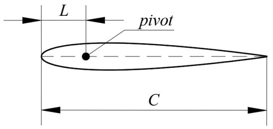
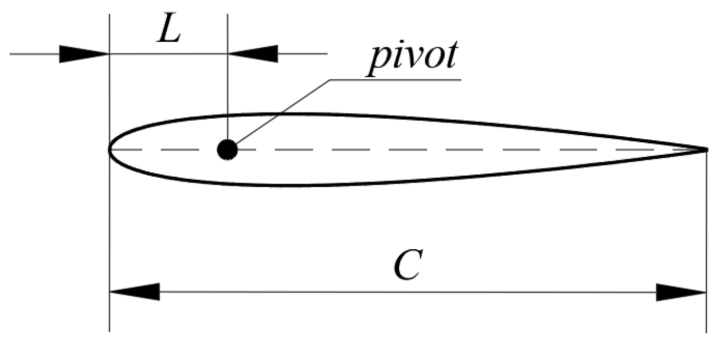
The numerical computation uses the NACA 0012 (a symmetric airfoil with 12% thickness-to-chord ratio) airfoil with a chord length of C = 1 m. According to previous studies [24], the optimal pumping efficiency is achieved when the pitching pivot is located at 0.2C. Therefore, in this study, the pivot position is set at L = 0.2C, as shown in Figure 1.

Figure 1. Hydrofoil geometry and parameters.

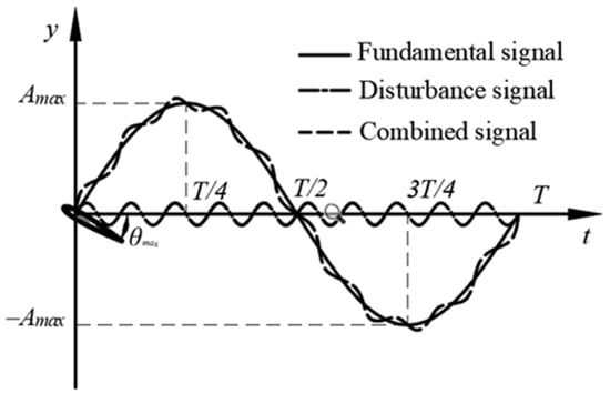
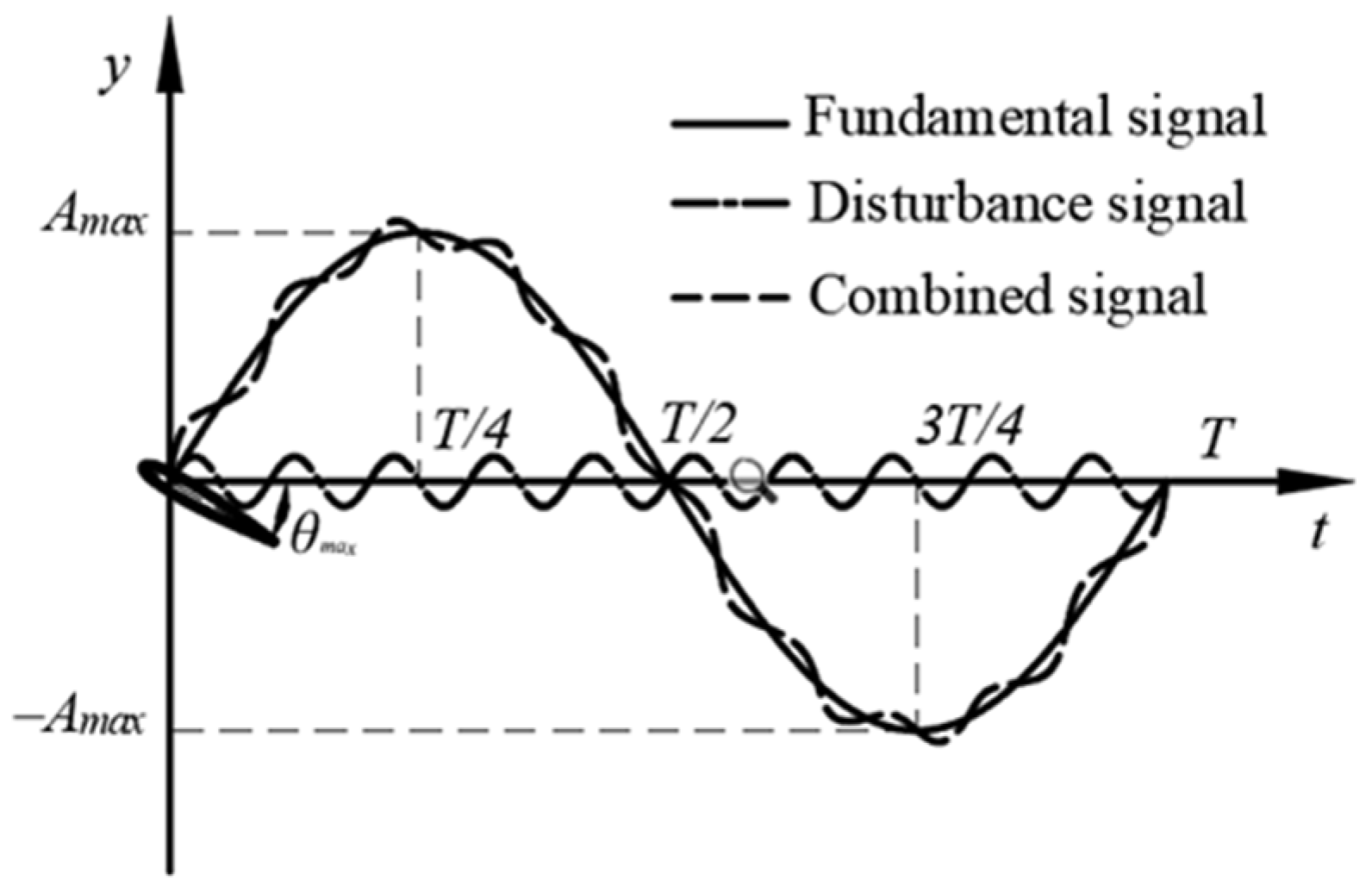
The hydrofoil kinematics consist of consists of two components: the heave translation of the pivot and the pitching rotation of the hydrofoil around the pivot, both of which vary sinusoidally. The prescribed input motion consists of a base component and a superimposed disturbance component. The base heave motion has an amplitude A = 0.45C and a frequency ranging from 0.25 to 1.75 Hz. The disturbance heave motion has an amplitude of 0.1A, with its frequency varying from 0 to 12 Hz. The motion is defined as follows:

$$\left\{\begin{array}{c}y\left(t\right)=A_{\max }\sin \left(2\pi f_{\mathrm{b}}t\right)+0.1A_{\max }\sin \left(2\pi f_{\mathrm{p}}t+{\phi }_1\right)\\ \theta \left(t\right)={\theta }_{\max }\sin \left(2\pi ft+{\phi }_2\right)\end{array}\right.$$

(1)

where y(t) is the hydrofoil heave displacement; θ(t) is the hydrofoil pitch angle; f_b and f_p are the base frequency and disturbance frequency, respectively; φ₁ is the phase offset between the base and disturbance signals, which is set to 0; and φ₂ represents the phase difference between the heave and pitch motions of the hydrofoil, which is set to −π/2. Figure 2 shows the waveform of the input signal.

Figure 2. Waveform of the input signal.

2.2. Performance Parameters

A rigid flat-plate hydrofoil is considered in this study, and its kinematics are prescribed by the following parameters: a heave amplitude of H_max = 0.45C and a pitch amplitude of θ_max = 30°. The Strouhal number (St) is introduced as a key dimensionless parameter to quantify the wake-flow dynamics associated with the hydrofoil motion:

$$St={\displaystyle \frac{2f{H}_{\max }}{U}}$$

(2)

where U is the magnitude of the incoming free-stream velocity.

The instantaneous thrust coefficient is defined by nondimensionalizing the thrust force generated during the oscillatory motion of the hydrofoil as follows:

$$C_T={\displaystyle \frac{2F_x(t)}{\rho U^{2}cs}}$$

(3)

Instantaneous lift coefficient:

$$C_L={\displaystyle \frac{2F_y(t)}{\rho U^{2}cs}}$$

(4)

where F_x(t) and F_y(t) represent the instantaneous thrust and lift forces, respectively; ρ is the fluid density; c is the chord length of the hydrofoil; and s is the hydrofoil span.

The thrust and lift coefficients averaged across several consecutive complete cycles:

$$\overline{C_T}={\displaystyle \frac{1}{KT}}{\displaystyle {\int }_{(n-k)T}^{nT}{C}_T}dt$$

(5)

$$\overline{C_L}={\displaystyle \frac{1}{KT}}{\displaystyle {\int }_{(n-k)T}^{nT}{C}_L}dt$$

(6)

where K denotes the number of cycles included in the averaging, and K is set to 2 in this study.

The propulsive performance of the flapping hydrofoil is characterized using the following parameters:

The mean volumetric flow rate at the outlet for the steady flow field is defined as

$$\overline{Q}=US$$

(7)

where S denotes the cross-sectional area of the flow channel.

The cycle-averaged input power is given by

$$\overline{P}={\displaystyle \frac{1}{T}}\left({\displaystyle {\int }_0^T{F}_y}(t)\dot{y}(t)dt+{\displaystyle {\int }_0^{T}M}(t)\dot{\theta }(t)dt\right)$$

(8)

where M(t) represents the instantaneous actuation torque.

The cycle-averaged power coefficient is defined as

$$\overline{C_p}={\displaystyle \frac{2\overline{P}}{\rho cs{U}^3}}$$

(9)

The propulsive efficiency is quantified as

$$\eta ={\displaystyle \frac{\overline{C_T}}{\overline{C_p}}}$$

(10)

The average power delivered to the fluid is given by

$$\overline{P_w}=\Delta \overline{P}\cdot \overline{Q}$$

(11)

where ∆$\overline{P}$ is the inlet–outlet pressure difference averaged over time.

The average head is defined as

$$\overline{H}={\displaystyle \frac{\Delta \overline{P}}{\rho g}}$$

(12)

The head averaged over a cycle is expressed as

$${\eta }_p={\displaystyle \frac{\overline{P_w}}{\overline{P}}}$$

(13)

2.3. Governing Equations and Turbulence Model Description

The computations were performed with ANSYS FLUENT-2024R2. For a two-dimensional incompressible viscous flow, the governing equations consist of the RANS momentum equations and the corresponding time-averaged continuity equation. The hydrofoil kinematics are specified by the following motion-control equations [25,26]:

$${\displaystyle \frac{\partial {\overline{u}}_i}{\partial x_i}}=0$$

(14)

$${\displaystyle \frac{\partial {\overline{u}}_i}{\partial t}}+{\overline{u}}_j{\displaystyle \frac{\partial {\overline{u}}_i}{\partial x_j}}=-{\displaystyle \frac{\partial \overline{p}}{\partial x_i}}+{\displaystyle \frac{\partial }{\partial x_j}}\left[(\gamma +{\gamma }_i)\left({\displaystyle \frac{\partial {\overline{u}}_i}{\partial x_j}}+{\displaystyle \frac{\partial {\overline{u}}_j}{\partial x_i}}\right)\right]$$

(15)

where $\overline{u}$_i (i = 1, 2) denotes the mean velocity components, x_i (i = 1, 2) are the Cartesian coordinates, p is the pressure, and t is the time. The kinematic viscosity is denoted by γ. The turbulent viscosity is given by γ_i = c_μk²/ε, where c_μ is a model constant, k is the turbulent kinetic energy, ε is the turbulent dissipation rate.

The propulsive performance of an oscillating hydrofoil is closely linked to vortex formation and shedding in the near-wake region. In order to achieve an adequate description of near-wall flow features consistent with the objectives of this study, the Realizable k-ε model is adopted for turbulence closure in solving the Reynolds-averaged Navier–Stokes equations.

2.4. Governing Equations and Turbulence Model

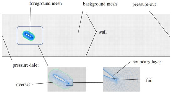
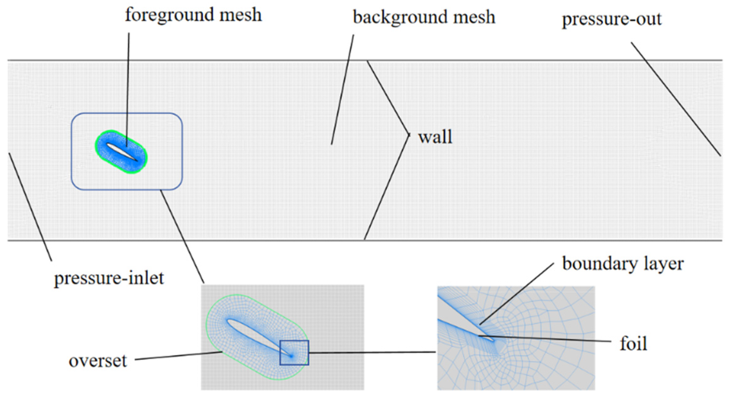
To reflect the intended application of the flapping-hydrofoil system in urban waterways of river-network regions, the computational domain is set to 20c × 5c, where c is the hydrofoil chord length. To resolve the downstream vortical structures while avoiding mesh distortion and negative cell volumes during the prescribed motion, the hydrofoil kinematics are implemented via User-Defined Functions (UDFs) in conjunction with an overset-mesh approach. As illustrated in Figure 3, the mesh system consists of a moving foreground grid and a stationary background grid. The foreground grid encloses the hydrofoil and moves according to the UDF-prescribed kinematics, whereas the background grid represents a rectangular channel domain. The boundary conditions are specified as a pressure inlet at the upstream boundary and a pressure outlet at the downstream boundary. An overset interface is applied at the outer boundary of the foreground grid, and no-slip conditions are imposed on the hydrofoil surface and the channel sidewalls.

Figure 3. Schematic of mesh generation.

To efficiently utilize computational resources while maintaining mesh quality, a hybrid meshing strategy was adopted in this study. In the vicinity of the flapping hydrofoil, structured meshes were generated to ensure high mesh quality and computational efficiency, whereas unstructured meshes were employed in the outer regions to better accommodate the complex geometry. The overset mesh region, corresponding to the flapping hydrofoil, is discretized using a hybrid mesh, while the background mesh region, representing the channel domain, is discretized using structured meshes. To ensure numerical accuracy and stability at the overset interfaces, the global base mesh size of the overset and background meshes was set to be identical.

Since turbulence models and wall functions impose specific requirements on the near-wall y+ values, boundary-layer grids were applied to the hydrofoil surface and channel walls. An enhanced wall treatment was adopted to improve the resolution of near-wall flow characteristics. By placing the first grid layer inside the viscous sublayer, this treatment provides enhanced near-wall resolution. The initial boundary-layer thickness was set to 0.0375 mm with a growth ratio of 1.2, resulting in y+ values < 1 over all simulated cases. The governing Navier–Stokes equations were solved using the pressure-based solver in ANSYS FLUENT. Pressure–velocity coupling was handled with the Coupled algorithm, and a first-order upwind scheme was employed for spatial discretization.

2.5. Grid Independence Verification

To guarantee the reliability of the simulations, the effects of mesh resolution and time-step size were examined through independence studies, and suitable settings were chosen based on convergence requirements. In this study, the case of a flapping wing with f_b = 0.25 Hz and f_p = 1 Hz is used as an example to perform grid and time step independence verification.

Regarding grid convergence, four sets of grid densities were selected for calculation, with the results shown in Table 1 and Table 2. The results indicate that as the grid density increases, the average thrust coefficient gradually decreases and stabilizes. The relative error between the third and fourth grid sets is approximately 0.9%, indicating that the calculation results become insensitive to further grid refinement. Therefore, considering both computational accuracy and cost, a grid size of 121,893 cells is chosen as the final grid configuration for subsequent calculations.

Table 1. Grid independence verification.

Number of Grids	$\mathbf{The} \mathbf{Average} \mathbf{Thrust} \mathbf{Coefficient} \overline{{\mathit{C}}_{\mathit{T}}}$
67,526	8.91
96,358	8.51
121,893	7.66
222,236	7.59

Table 2. Time step independence verification.

Time Step	$\mathbf{The} \mathbf{Average} \mathbf{Thrust} \mathbf{Coefficient} \overline{{\mathit{C}}_{\mathit{T}}}$
$\Delta t=T/10$	9.23
$\Delta t=T/50$	8.63
$\Delta t=T/100$	7.66
$\Delta t=T/1000$	7.55

A time-step sensitivity analysis was performed to evaluate the impact of temporal discretization on the numerical results. Four time-step sizes, decreasing progressively, were tested for the same operating condition. The average thrust coefficients obtained with the four time-step sizes are 9.23, 8.63, 7.66, and 7.55, respectively. The results reported in Table 2 suggest that as the time step size decreases, the average thrust coefficient gradually converges and stabilizes. When the time step size is reduced to the third and fourth sets, the difference between them is less than 1.5%, suggesting that the time integration error is small, and further decreasing the time step size has minimal impact on the results. Considering both accuracy requirements and computational cost, a time step size from the third group is selected as the time discretization parameter for subsequent calculations.

2.6. Validation of Numerical Methodology

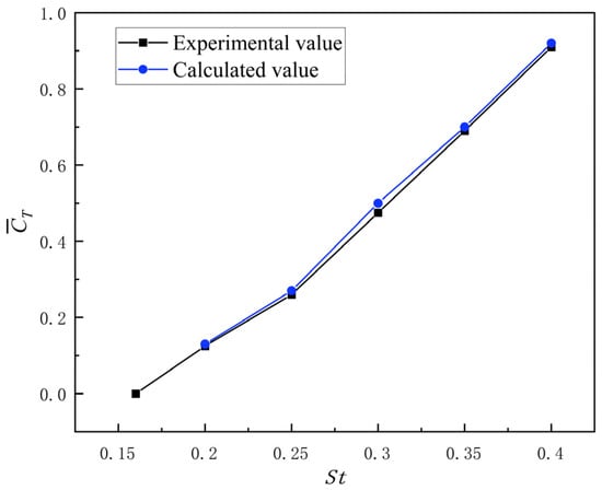
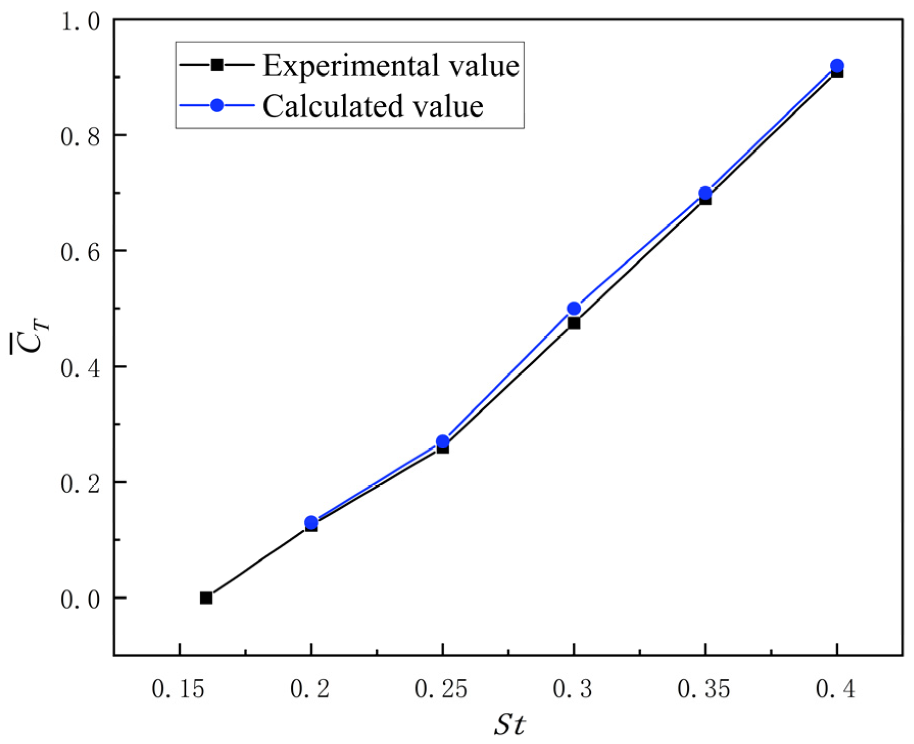
To validate the reliability of the numerical simulation method, a simulation model for the same operating conditions was established based on the experimental study of the NACA 0012 airfoil conducted by Schouveiler et al. [16] in the towing tank at the MIT. The computed results were then compared with their experimental data. The inflow velocity was 0.4 m/s, the maximum angle of attack was θ_max = 30°, the phase was φ = −π/2, and the heave amplitude was A_max = C = 0.1 m. The curve of the average thrust coefficient of the oscillating hydrofoil as a function of the Strouhal number (St) was compared with the experimental data from the literature. As illustrated in Figure 4, the predicted mean thrust coefficient agrees well with the experimental data, indicating good consistency and supporting the validity of the numerical approach adopted in this study.

Figure 4. Comparison of numerically predicted thrust with experimental data from the literature.

3. Analysis of Computational Results

Since there is a significant difference between f_b and f_p, it is not appropriate to determine the computational period based solely on either of the frequencies. Accordingly, the simulation time window is defined based on a common period that accommodates both the base and disturbance motions. Specifically, the least common multiple of the base-motion period and the disturbance-motion period is adopted as the fundamental computational period. For instance, with a base frequency of 0.5 Hz and a disturbance frequency of 10 Hz, the resulting computational period is 2 s. The total simulation duration is set to ten times this period to ensure a statistically periodic response, and the reported results are obtained by averaging over the last two computational periods.

3.1. Effect of High-Frequency Disturbance on Flapping Wing Propulsion Performance

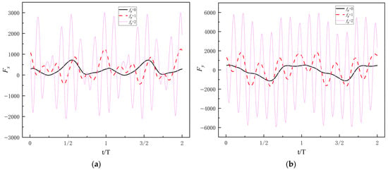
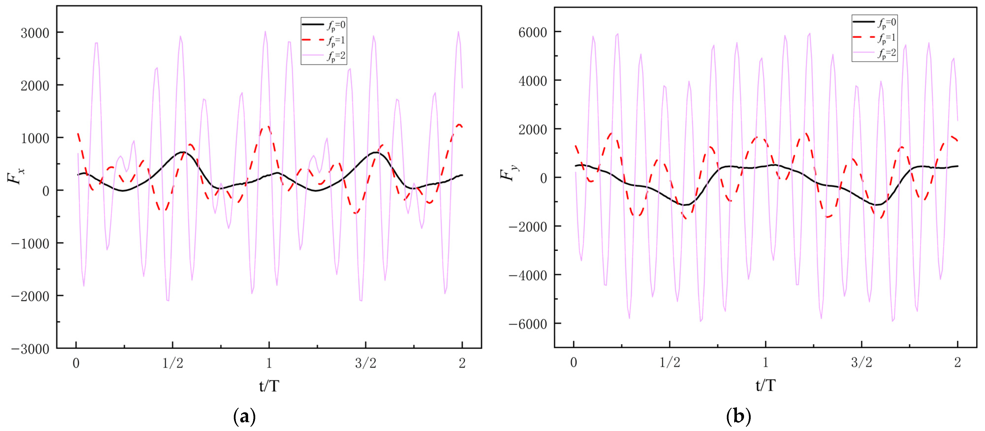
Since the temporal evolution of the instantaneous thrust under different disturbance frequencies is generally similar—namely, a high-frequency oscillation superimposed on the base frequency—representative cases with f_b = 0.25 Hz and f_p = 0, 1, 2 Hz are selected for analysis. The corresponding instantaneous thrust histories are shown in Figure 5. It can be seen that, when f_p = 0 Hz, the instantaneous thrust remains positive over the entire cycle, indicating that the flapping wing continuously exerts a propulsive effect on the flow during its motion. After the disturbance is introduced, the thrust begins to fluctuate between positive and negative values, and as the disturbance frequency increases, both the number of oscillations and their amplitudes increase. This indicates that the disturbance enhances the instantaneous unsteadiness of the pressure field, causing the hydrofoil to experience more frequent thrust reversals within a single cycle.

Figure 5. Instantaneous thrust and lift under different disturbance frequencies: (a) Instantaneous thrust under different disturbance frequencies; (b) Instantaneous lift under different disturbance frequencies.

From the viewpoint of periodicity, the overall period of the thrust signal is still determined by the base frequency f_b = 0.25 Hz; in other words, the fundamental period remains unchanged. The introduction of the disturbance causes the instantaneous thrust to contain both the base frequency and the disturbance frequency as two distinct time scales, whose superposition produces a characteristic amplitude-modulated waveform: the thrust envelope is governed by the base frequency, while the high-frequency component associated with the disturbance repeatedly modulates the magnitudes of the thrust peaks and troughs within each fundamental cycle. This multi-frequency coupled structure reflects the pronounced modulation of local thrust and vortex shedding rhythm by the disturbance.

In addition, since both lift and thrust originate directly from variations in the instantaneous pressure distribution over the foil surface, the modulation of vortex shedding and attached flow by the disturbance acts simultaneously on both force components. As can be seen from the figure, the instantaneous lift histories under the three disturbance cases exhibit evolution patterns that are highly similar to those of the instantaneous thrust.

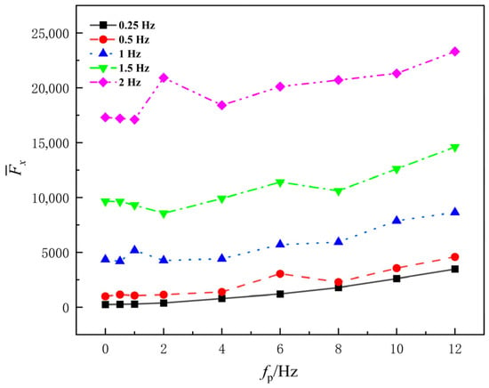
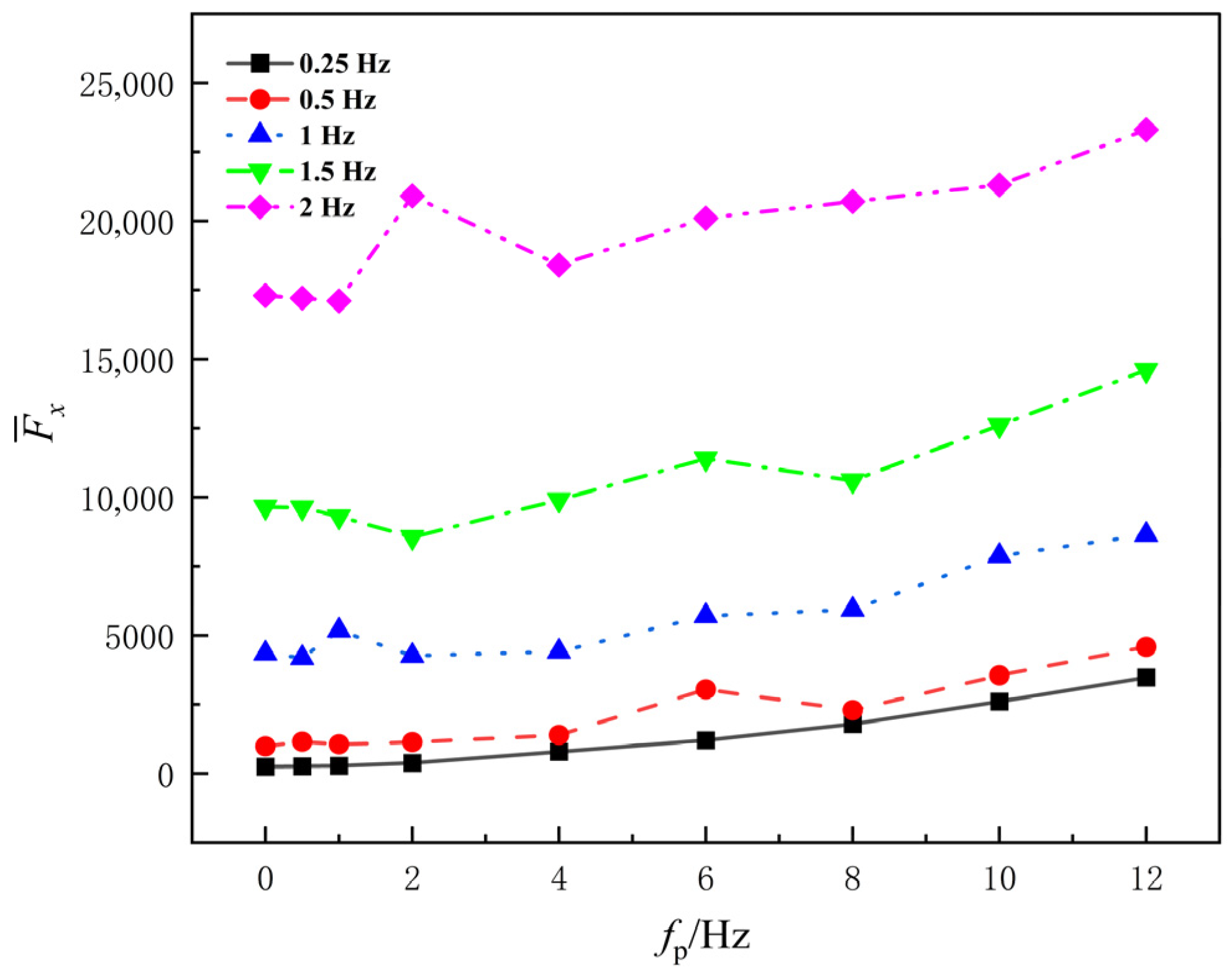
Figure 6 shows the variation in average thrust with disturbance frequency f_p for a heave–pitch flapping wing at different base frequencies f_b. When f_p = 0 Hz, it means that the input signal is solely determined by the base signal, serving as a control group to facilitate the investigation of the impact of the disturbance signal on the flapping wing’s thrust coefficient.

Figure 6. Average thrust under different fundamental frequencies.

Overall, after high-frequency disturbances are superimposed on the heave–pitch motion, the average thrust of the hydrofoil increases with the disturbance frequency. When the disturbance frequency f_p < 2 Hz, the average thrust changes little, and the curves for different base frequencies remain relatively flat. This indicates that, in this range, high-frequency disturbances have a limited effect on fluid momentum exchange. When the disturbance frequency f_p ≥ 2 Hz, the average thrust starts to increase significantly. This suggests that once the disturbance frequency exceeds a certain threshold, the unsteady interaction between the hydrofoil and the fluid is enhanced, strengthening the wake vortex structure and thereby increasing thrust output.

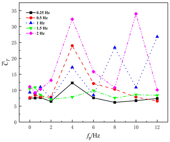
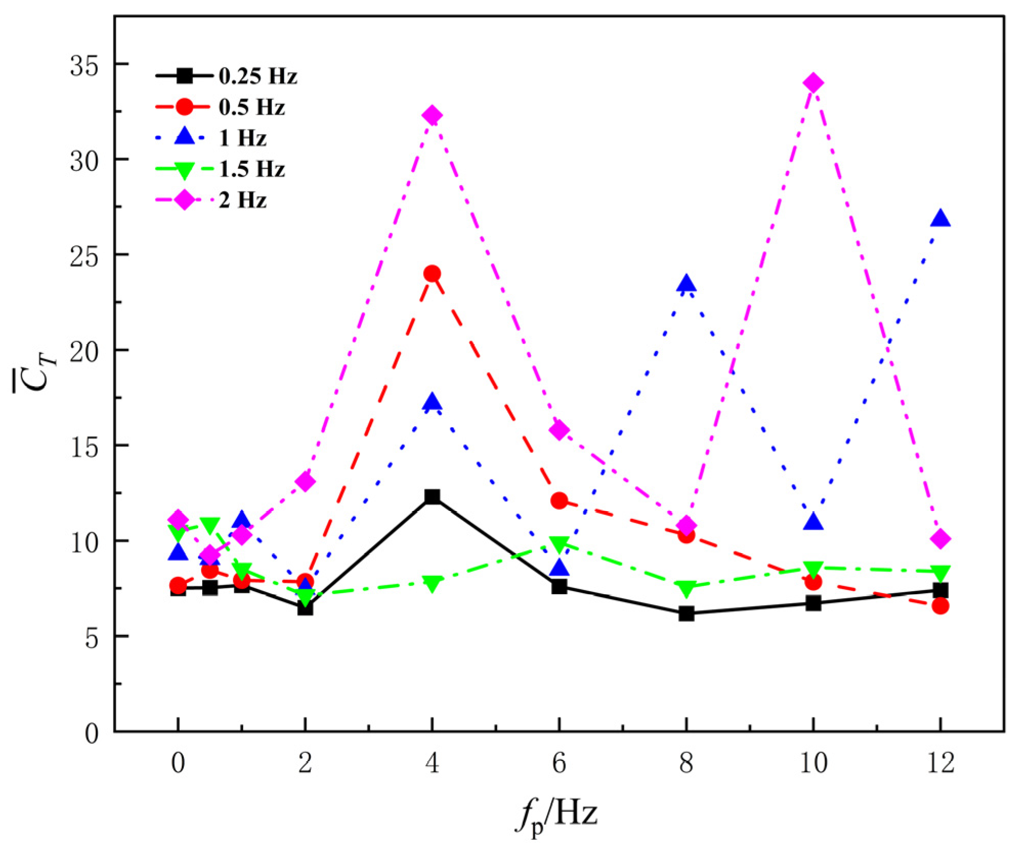
In pumping applications for small river basins, the thrust coefficient is an important indicator for evaluating hydrofoil performance, as it effectively reflects the relative efficiency of the thrust generated by the hydrofoil. Figure 7 shows the variation in the average thrust coefficient C_T with the disturbance frequency f_p for the flapping wing at different base frequencies f_b. As seen from the figure, the average thrust coefficient changes little in the low disturbance frequency range (0–2 Hz). When f_p > 2 Hz, the curves for all base frequencies show fluctuations and local peaks, especially at higher base frequencies, where the amplitude of the thrust coefficient increases significantly, exhibiting a stronger frequency response characteristic. Since the chord length and amplitude are kept constant in this study, the significant changes in the thrust coefficient are mainly attributed to the dynamic changes in the fluid velocity field and vortex structure. When the disturbance frequency is low, the effect of the disturbance on the flow field is limited, the wake structure remains relatively stable, and the variations in thrust and flow velocity are small, resulting in little change in the coefficient. However, when the disturbance frequency exceeds a certain threshold, the unsteady effects of the fluid are enhanced, and the interaction between the leading-edge vortex and wake becomes more frequent, causing significant fluctuations in instantaneous thrust and local flow velocity. At this point, due to the faster increase in outlet velocity, the increase in the normalized denominator ${\overline{U}}^2$ may surpass the thrust growth, leading to a decrease in the coefficient in certain regions. Therefore, high-frequency disturbances do not merely increase thrust, but also alter the manner in which momentum is exchanged between the hydrofoil and the fluid.

Figure 7. Average thrust coefficient under different fundamental frequencies.

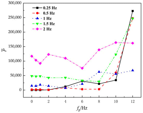
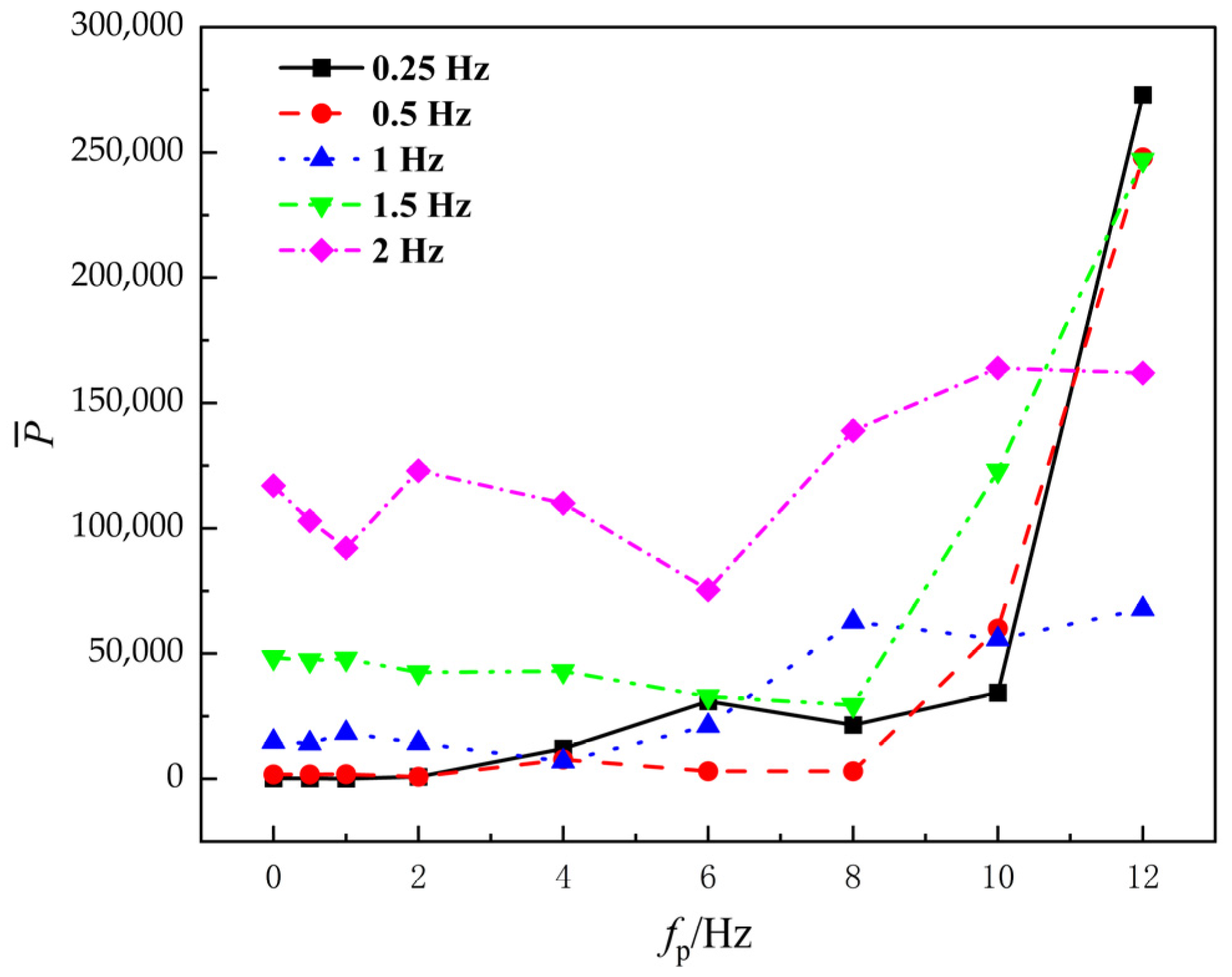
Figure 8 shows the variation in the average input power with disturbance frequency f_p for the flapping wing at different base frequencies f_b. As seen from the figure, when f_p ≤ 6 Hz, the overall level of average input power remains low, with limited variation as f_p changes. Some curves even show a slight decrease, indicating that, at this stage, the high-frequency disturbance has little effect on amplifying the hydrofoil’s velocity and acceleration, and the increase in driving energy consumption is minimal. However, when f_p > 6 Hz, the average input power increases significantly, especially for f_b = 0.25, 0.5, 1.5 Hz. At f_p = 10∼12 Hz, the power shows a nearly “steep increase” trend. It is important to note that, although the increased input power results in higher thrust output, energy losses due to vortex formation and turbulence dissipation in the wake region may prevent the power consumption from being fully converted into effective thrust.

Figure 8. Average input power under different fundamental frequencies.

Figure 9 shows the variation in propulsion efficiency with disturbance frequency f_p for the flapping wing at different base frequencies f_b. As seen from the figure, when f_p ≤ 2 Hz, efficiency for most base frequencies remains within the range of 25–35%, with little variation. Only for f_b = 0.25 Hz, a peak value of 70.8% is observed. This is due to the fact that, in this case, the average input power is minimized while thrust slightly increases, leading to “local high efficiency.” For f_p > 2 Hz, the propulsion efficiency fluctuates more significantly across different base frequencies, and the specific reasons for this are analyzed in Section 3.3.

Figure 9. Propulsive efficiency under different fundamental frequencies.

3.2. Effect of High-Frequency Disturbance on the Pumping Performance of Flapping Wings

In small river basins, flow rate, pressure difference, and input power are all key factors influencing pumping efficiency. To better understand the reasons behind efficiency changes under different operating conditions, this study analyzes the variations in these factors under different disturbance frequencies.

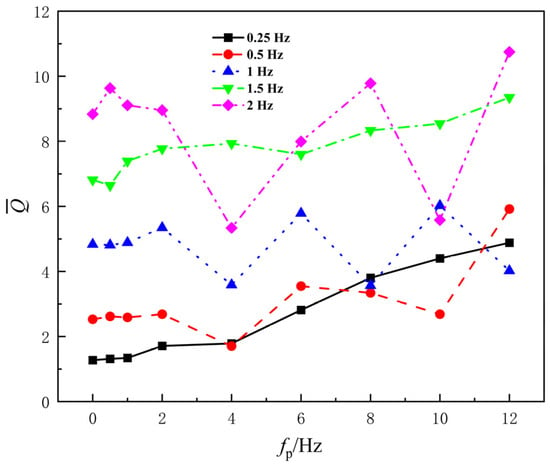
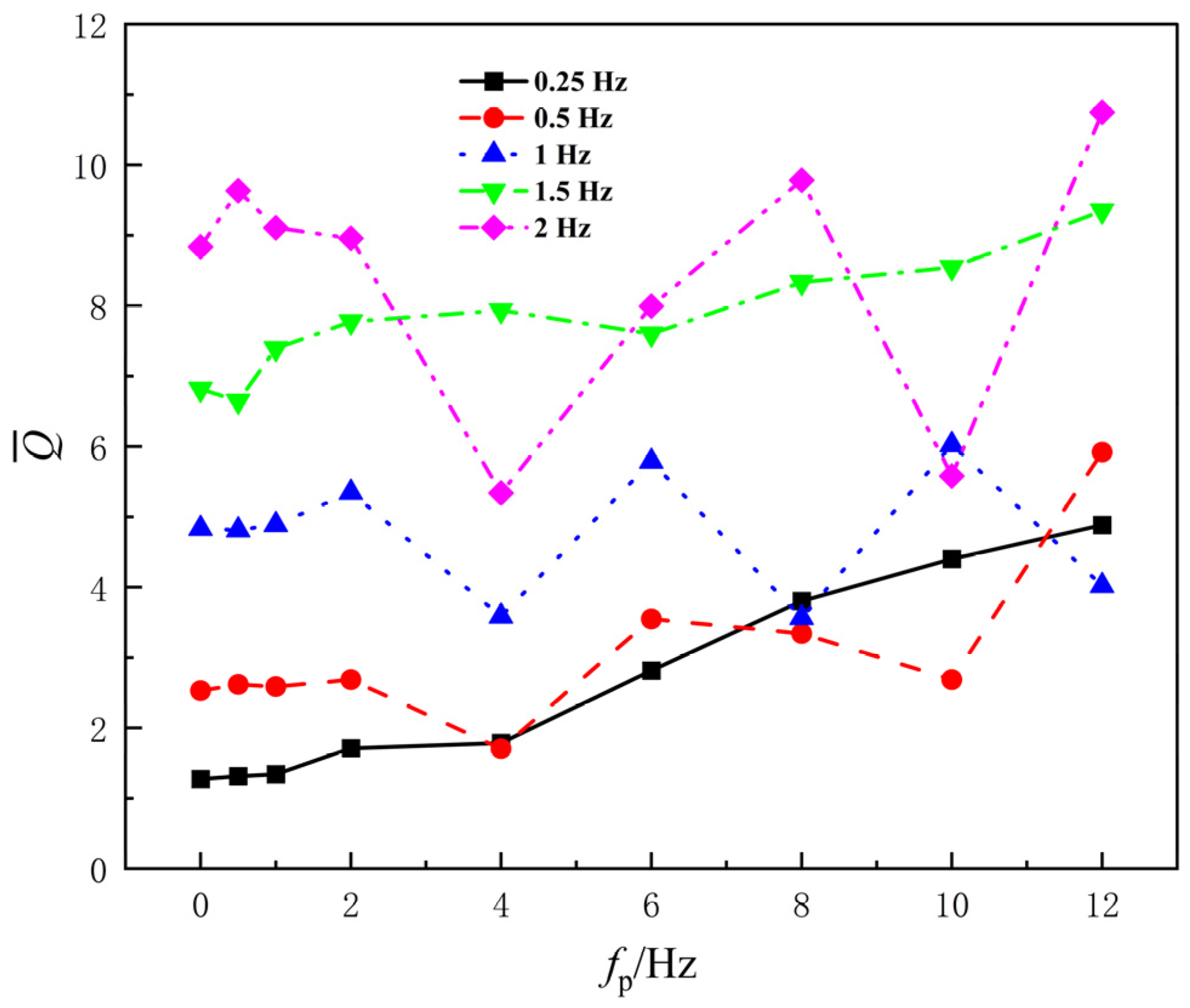
Figure 10 shows the variation in flow rate with disturbance frequency f_p for different base frequencies f_b. As seen in the figure, at low base frequencies of 0.25 and 0.5 Hz, the flow rate increases gradually with disturbance frequency, with relatively small changes in the middle-low disturbance frequency range. A more noticeable increase occurs at higher disturbance frequencies. At higher base frequencies of 1.5 and 2 Hz, the overall flow rate is the highest, and it increases gradually with f_p. However, a significant decrease is observed at f_p = 4 Hz, after which it continues to increase. The 1 Hz curve lies between these two cases, showing an overall increasing trend, but with some decreases at specific disturbance frequencies. The flow rate increases progressively with disturbance frequency, indicating that high-frequency disturbances indeed enhance the average momentum transport within the channel; however, at disturbance frequencies near that of the pressure difference (around 4 Hz), there is a local reduction, suggesting that the wake structure in this frequency range is not conducive to forming maximum flow.

Figure 10. Flow rate under different fundamental frequencies.

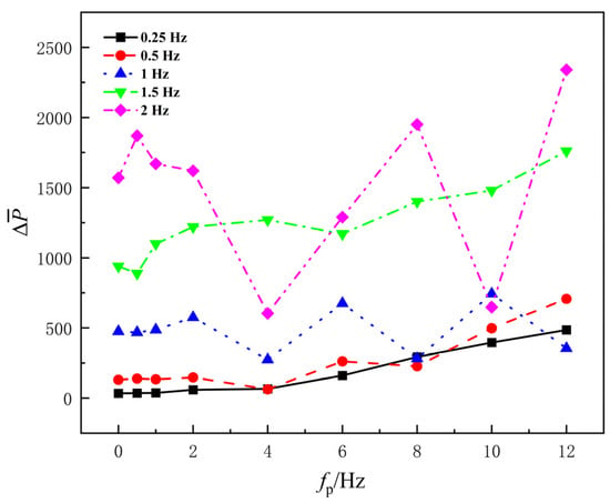
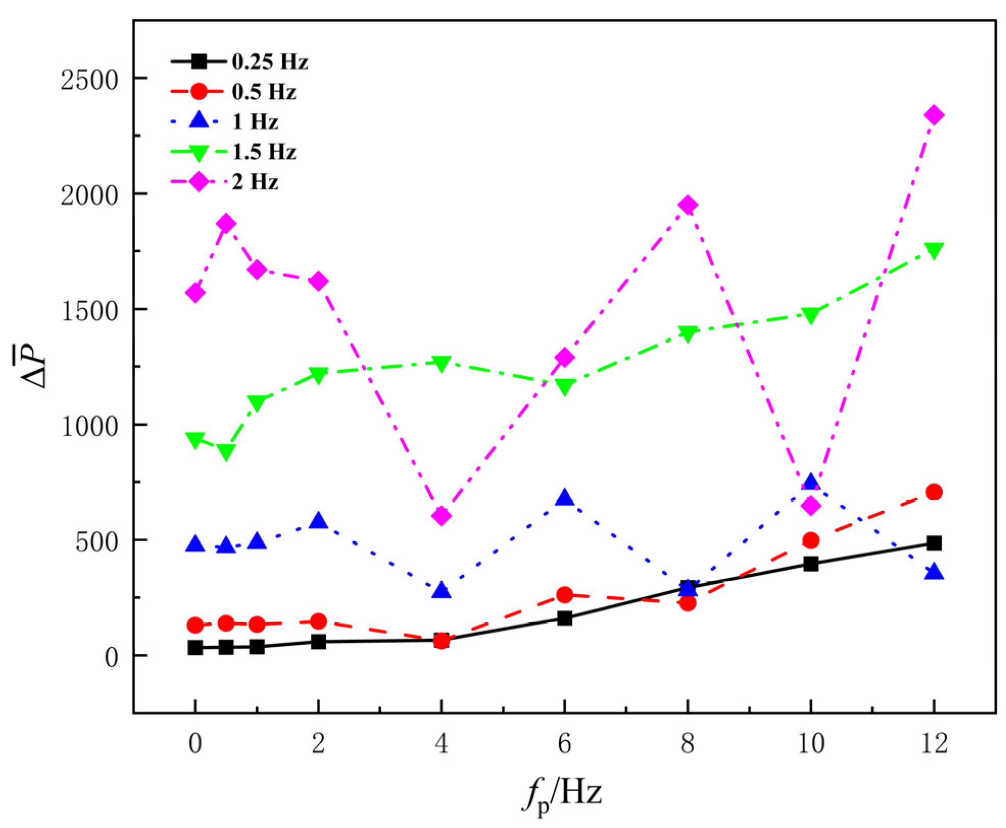
Figure 11 shows the variation in pressure difference with disturbance frequency f_p for different base frequencies f_b. At low base frequencies of 0.25 and 0.5 Hz, the average pressure difference increases monotonically but slowly with disturbance frequency, remaining relatively low. This indicates that high-frequency disturbances gradually enhance the pressure rise at low base frequencies, but the overall level is limited. At higher base frequencies of 1, 1.5, and 2 Hz, the absolute value of pressure difference is significantly higher and increases overall, with local sharp fluctuations. However, at f_p = 4 Hz, both the 1 Hz and 2 Hz curves show a clear “valley.” As the disturbance frequency increases, the pressure difference quickly recovers. This suggests that as the disturbance frequency increases, the pressure difference generated by the hydrofoil increases overall, especially at higher base frequencies. At f_p = 4 Hz and f_b = 2 Hz, the pressure difference significantly weakens, indicating that at this point, the vortex structure or wake morphology undergoes a rearrangement that is detrimental to pressure rise.

Figure 11. Pressure difference under different fundamental frequencies.

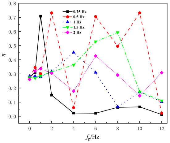
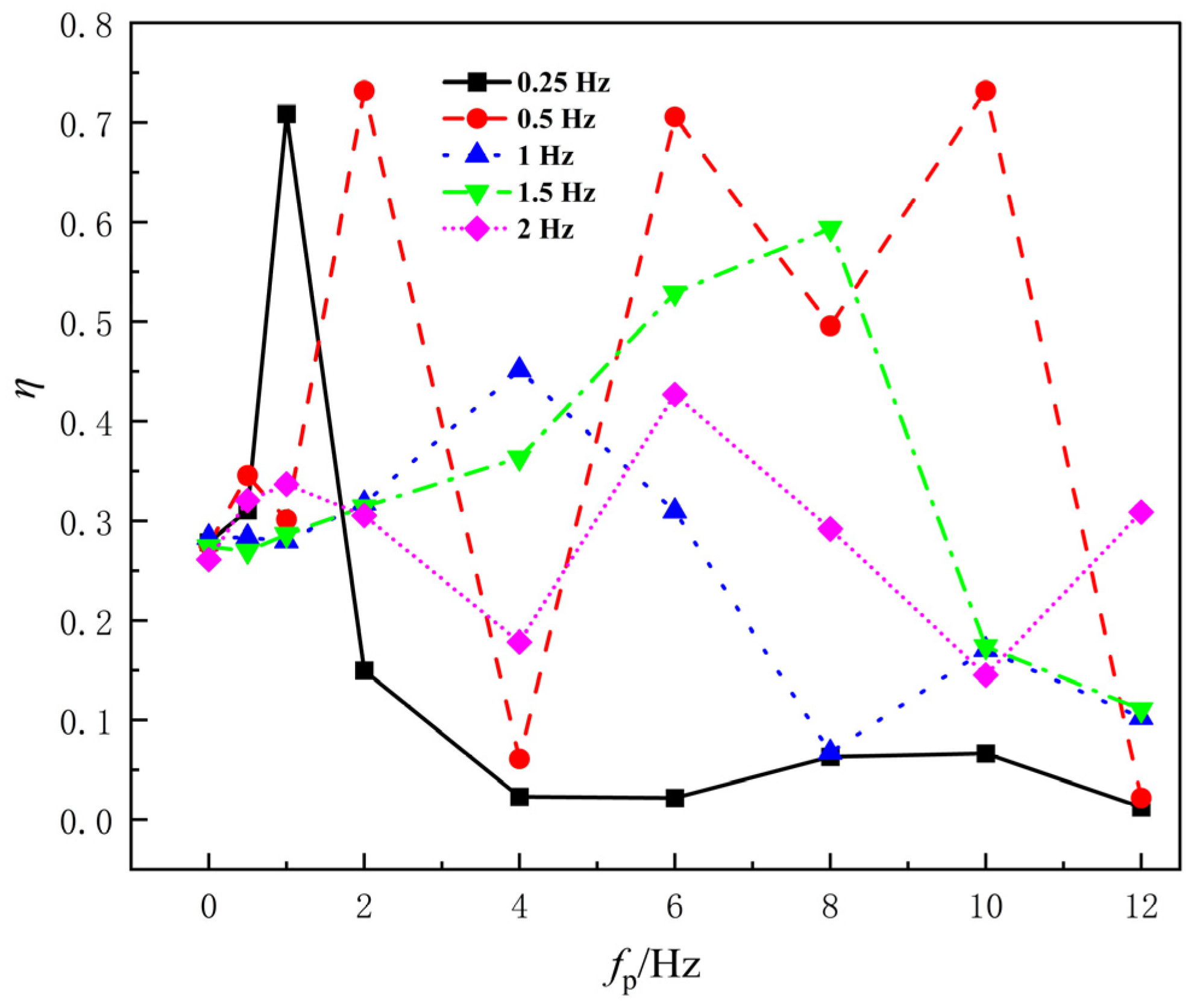
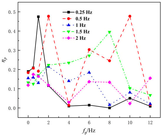
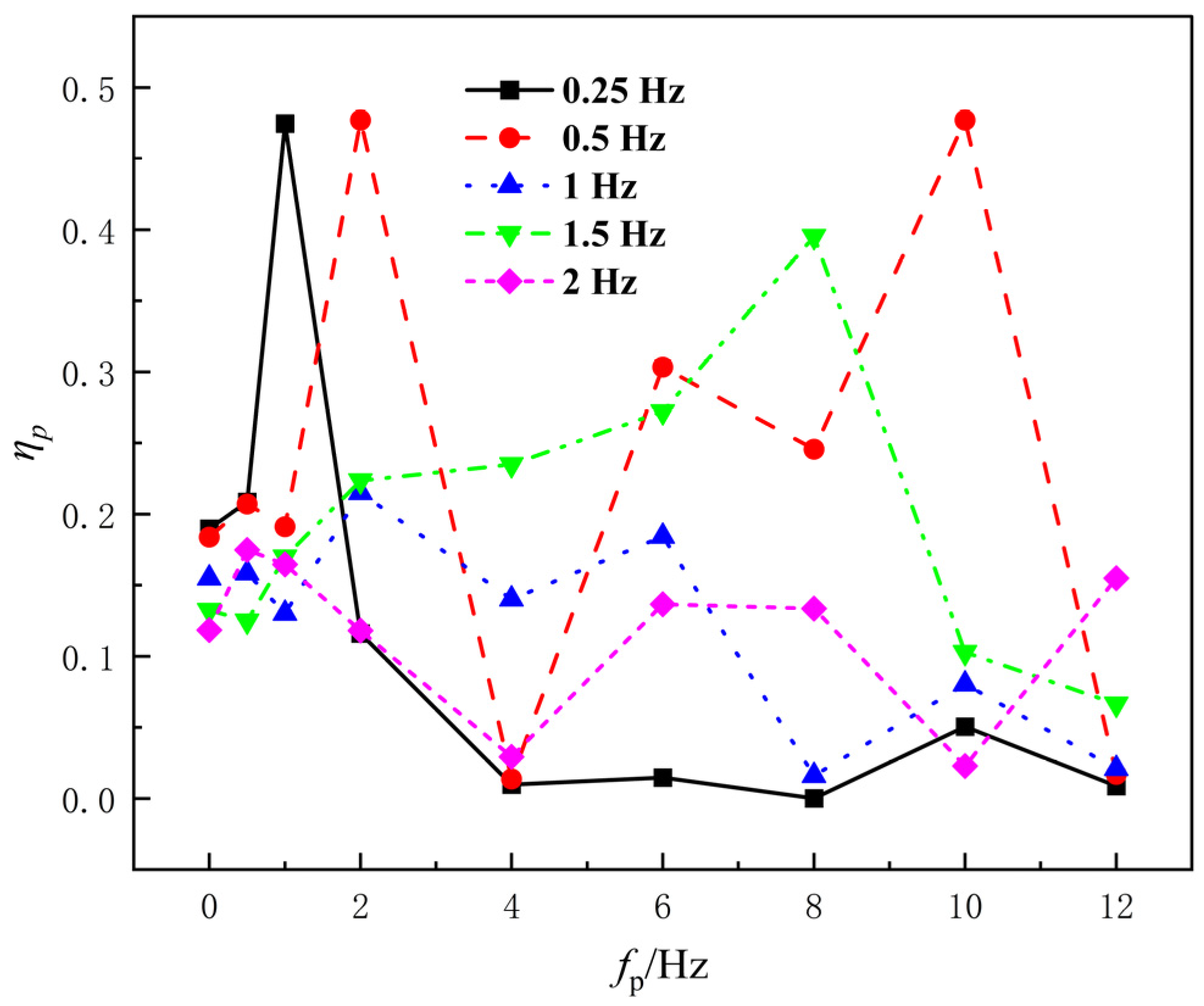
Figure 12 presents the pumping efficiency η as a function of the disturbance frequency f_p for different base frequencies f_b. Overall, the efficiency curves exhibit significant fluctuations at each base frequency, indicating that pumping efficiency is influenced by the combined effects of pressure difference, flow rate, and input power under disturbance driving, with a marked nonlinear variation. Similarly to the trend observed for propulsion efficiency, when f_p ≤ 2 Hz, for most base frequencies, the efficiency remains within the range of 25–35%. An anomalous peak is observed at f_b = 0.25 Hz, where the input power is still relatively low, and the pressure difference and flow rate show slight increases, temporarily raising the efficiency to a higher level. At f_b = 0.5 Hz, efficiency peaks occur at both f_p = 2 Hz and f_p = 2 Hz, with the latter reaching 47%, the highest of all conditions. At f_b = 1.5 Hz, efficiency gradually increases with f_p, peaking at 39% at f_p = 8 Hz. For the conditions with base frequencies f_b = 1 Hz and f_b = 2 Hz, the changes in pumping efficiency with increasing disturbance frequency are notably weaker than at the other base frequencies, and the overall curves are relatively flat.

Figure 12. Pumping efficiency under different fundamental frequencies.

3.3. Effect of High-Frequency Disturbance on Flow Field Structure

To further investigate the impact of disturbance signals on the propulsion performance of the flapping wing, this study selected three representative base frequencies—namely, 0.5 Hz, 1.5 Hz, and 2 Hz—from five base frequency groups for flow field analysis. These three base frequencies correspond to low, medium, and high ranges of unsteady intensity, respectively. Their wake structures and responses to disturbance frequencies exhibit significant differences, making them suitable for fully characterizing the effects of disturbance signals.

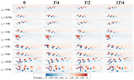
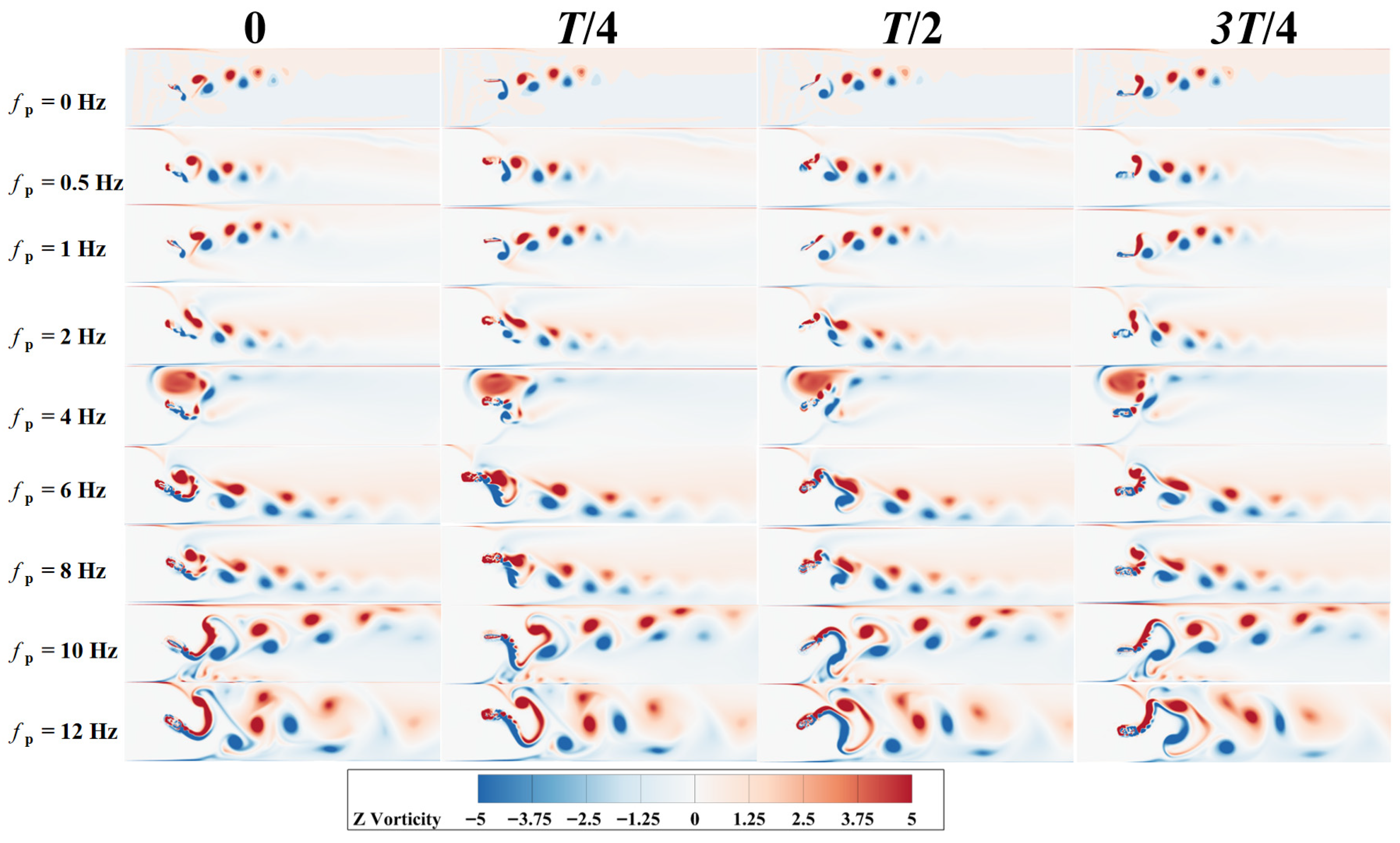
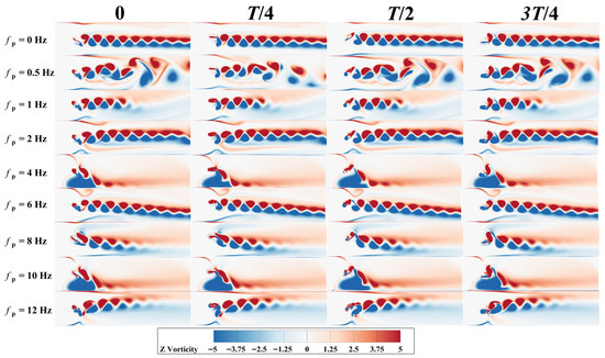
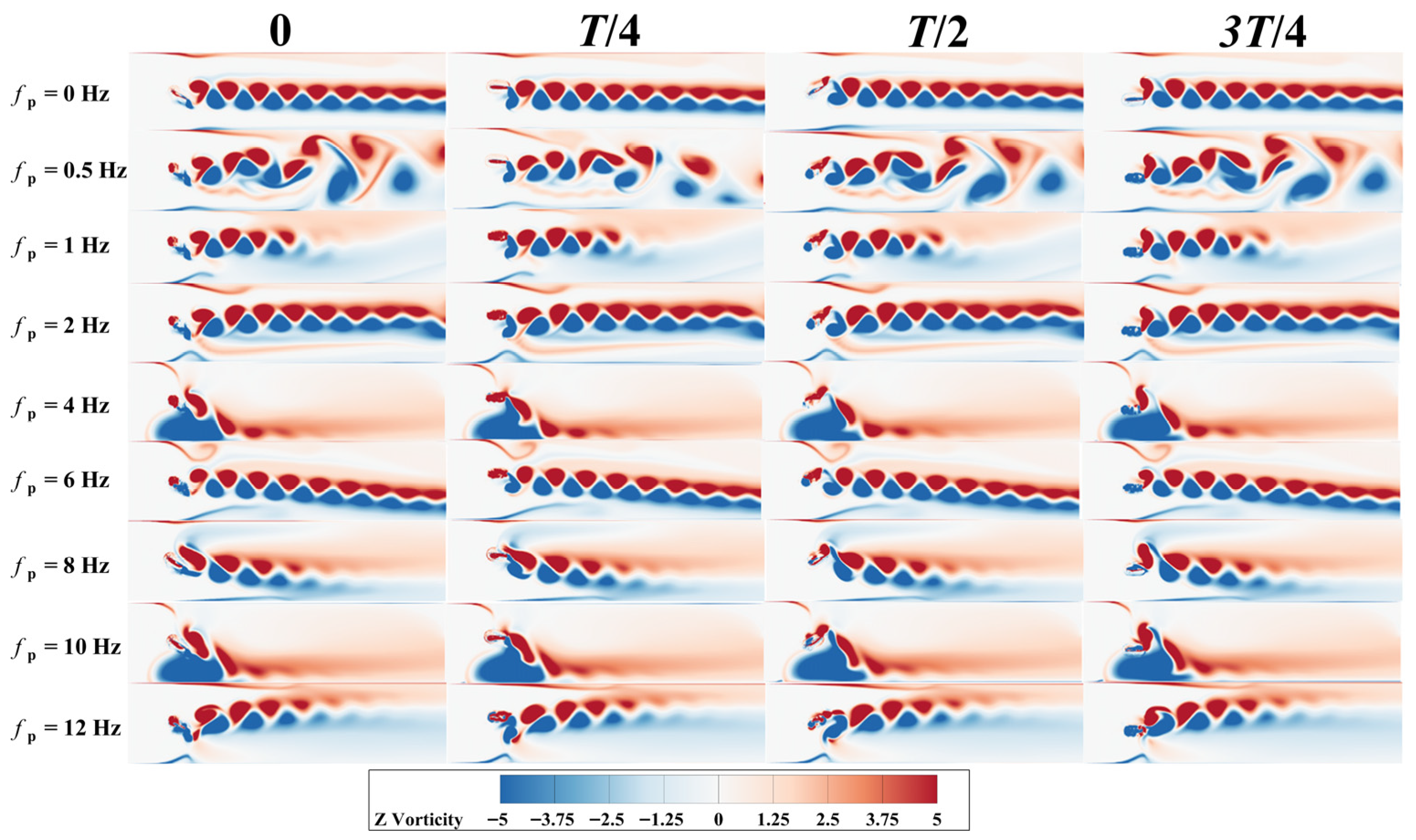
Figure 13 shows the variation in wake vortex structure with disturbance frequency f_b when f_b = 0.5 Hz. As seen from the figure, when f_b = 0 Hz, the wake structure of the flapping wing exhibits a typical Kármán vortex street pattern. During the T/4 phase, a clockwise vortex generated at the trailing edge of the hydrofoil detaches and moves along the lower surface of the wing. By the time the motion reaches T/2, the trailing edge gradually forms a counterclockwise vortex, but the vortex has not yet detached. As the motion progresses to 3 T/4, the counterclockwise vortex formed earlier detaches along the upper surface of the hydrofoil, forming an opposite-rotation Kármán vortex pair with the previous clockwise vortex. These vortices interlace and gradually form a vortex street in the wake, but their vortex energy dissipates quickly. As the hydrofoil completes the cycle and returns to its starting position, a clockwise trailing-edge vortex appears again.

Figure 13. Wake vortex structure of the flapping wing at f_b = 0.5 Hz.

When f_p = 0.5 Hz and f_p = 1 Hz, the disturbance causes the shed vortices to be slightly stronger, but the overall structure still maintains the Kármán vortex street pattern. This aligns with the trend of slight increases in pressure difference and flow rate, and little change in efficiency under low disturbance frequencies. When f_p = 2 Hz, the vortex structure starts to show slight asymmetry, with a slightly shortened shedding pitch and an increase in vortex strength, but no obvious multi-scale vortex structure is formed.

At f_p = 4 Hz, the vortex street is clearly displaced, causing a “joint valley” in both pressure difference and flow rate, at which point the pumping efficiency is at its lowest. When f_p = 6, 8, 10 Hz, the wake structure is significantly reinforced. During this phase, both pressure difference and flow rate increase significantly, while input power remains moderate, leading to high pumping efficiency.

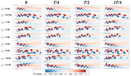
Figure 14 shows the variation in the wake vortex structure with disturbance frequency f_p when f_b = 1.5 Hz. Compared to low base frequencies (e.g., 0.5 Hz), the wake vortex structure at f_b = 1.5 Hz is more sensitive, exhibiting stronger unsteady vortex generation, entrainment, merging, and shedding phenomena. At f_p = 1.5 Hz, the wake initially forms a nearly symmetric double vortex street near the trailing edge of the hydrofoil, indicating that vortex shedding is still dominated by the base frequency. As the vortex structure is transported downstream, adjacent vortices merge significantly, and the wake evolves from a symmetric vortex street to a larger-scale composite vortex structure. Notably, this composite vortex structure does not increase flow rate and pressure difference, and even causes a slight decrease in pumping efficiency.

Figure 14. Wake vortex structure of the flapping wing at f_b = 1.5 Hz.

At f_p = 8 Hz, the wake vortex field shows numerous small-scale vortex structures and exhibits significant incoherence, with no jet formation. At this point, pressure difference and flow rate show limited changes. However, at this disturbance frequency, the hydrofoil’s overall acceleration effect on the surrounding fluid weakens, and the unsteady inertial work related to added mass decreases accordingly, resulting in a lower average input power than at nearby disturbance frequencies. Consequently, the pumping efficiency reaches its maximum value of 39%. When f_p = 10 Hz and f_p = 12 Hz, due to the increase in average input power, and the growth rate of input power far exceeding that of pressure difference and flow rate, pumping efficiency drops sharply.

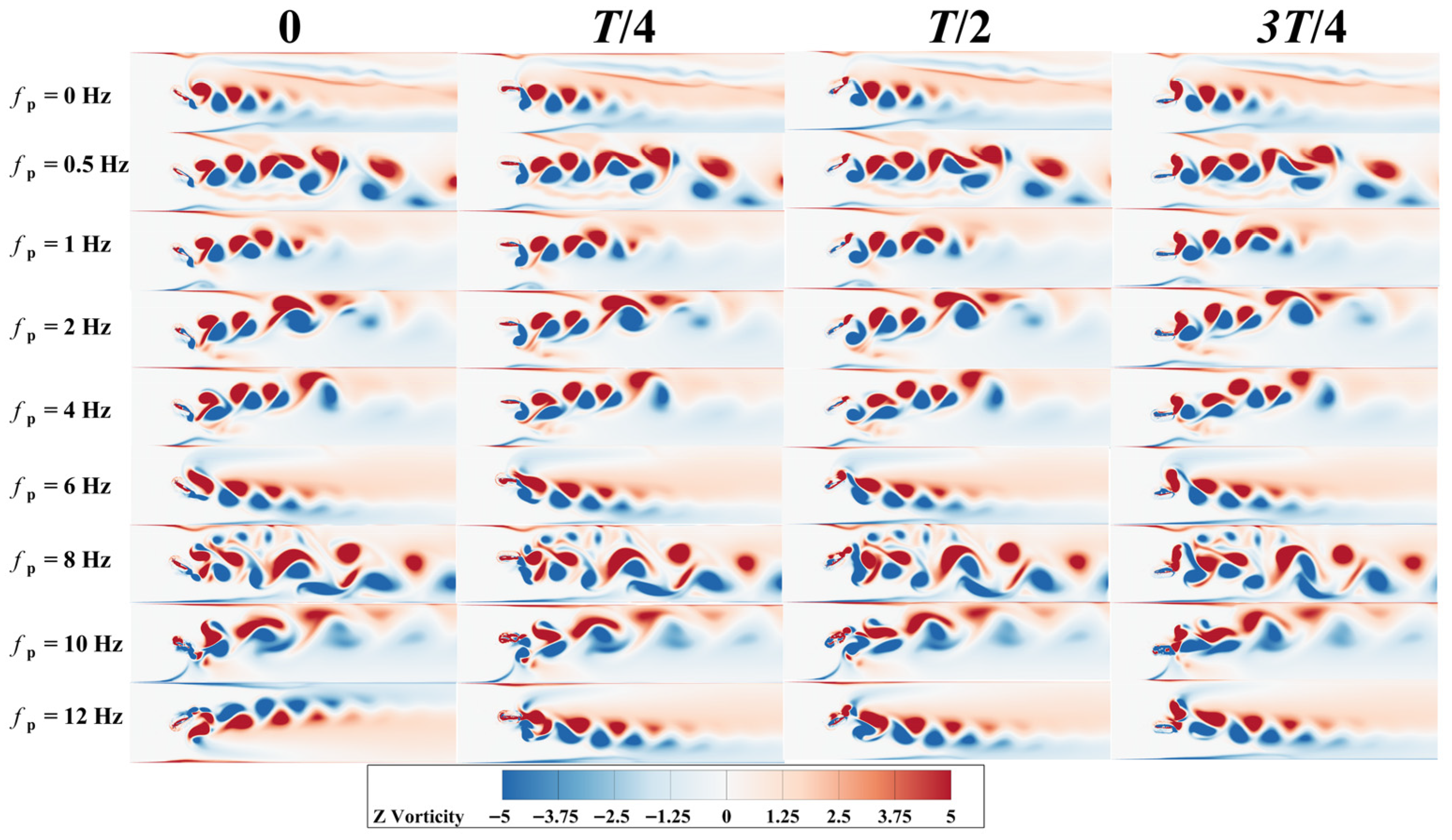
Figure 15 compares the wake vortex structures at different disturbance frequencies f_p for a fixed base frequency of f_b = 2 Hz. As analyzed earlier, the pumping efficiency of the hydrofoil at this base frequency remains below 20%. When f_p = 0.5 Hz, the wake initially forms a symmetric vortex street, and later, vortex pairs merge to form stronger vortices, which causes a moderate increase in flow rate and pressure difference in the channel. At this point, the average input power decreases compared to the previous two conditions, resulting in the maximum pumping efficiency of 17.5%. At f_p = 4 Hz and f_p = 10 Hz, lower pumping efficiencies are observed. Analysis of the vortex cloud maps reveals that the vortex street in the wake shifts toward the wall, where the vortices interact strongly with the wall boundary layer, leading to vortex stretching and vortex dissipation. This prevents the formation of a concentrated and stable jet, causing a significant decrease in outlet pressure difference and flow rate, while the input power remains at a certain level, ultimately leading to a decrease in pumping efficiency.

Figure 15. Wake vortex structure of the flapping wing at f_b = 2 Hz.

Additionally, since both propulsion efficiency and pumping efficiency share the same input power in the denominator, and their numerators are both derived from outlet flow rate, they actually reflect the energy utilization level under the same flow mechanism. Therefore, the variations in both types of efficiency with disturbance frequency exhibit a high degree of consistency.

4. Conclusions and Outlook

In this study, high-frequency disturbances in the heave direction are introduced based on the fundamental heave–pitch motion. Using overlapping grid technology and the Realizable k-ε turbulence model, the forces on the flapping wing, flow field structure, and pumping performance are investigated. The main conclusions are as follows:

• The introduction of disturbances causes the instantaneous thrust to contain both the base frequency and disturbance frequency as two times scales. Their superposition forms a characteristic amplitude-modulated waveform, where the base frequency determines the overall cycle of thrust generation, while the disturbance frequency introduces f_p/f_b fast oscillations within each base frequency cycle, resulting in the characteristic amplitude modulation. As the disturbance frequency increases, the average thrust of the flapping wing also increases.
• In the low disturbance frequency range (f_p/f_b ≤ 16), the high-frequency disturbance has little effect on the average thrust, pressure difference, and flow rate. Instantaneous thrust and lift exhibit only slight high-frequency oscillations dominated by the base frequency, and the pumping efficiency shows limited changes.
• In the intermediate disturbance frequency range (16 < f_p/f_b ≤ 32), the wake of the hydrofoil transitions from a symmetric or weak vortex street structure to a more coherent vortex chain and jet-like structure. Thrust, pressure difference, and flow rate increase synchronously, while the input power has not yet risen sharply. The pumping efficiency and thrust efficiency reach their peak in this range, with a maximum of 47%, and there exists an optimal disturbance frequency corresponding to the base frequency.
• In the high disturbance frequency range (f_p/f_b > 32), the vortex scale and intensity further increase, but the wake gradually shows multi-scale, highly unsteady, and even chaotic characteristics. The average input power increases rapidly, and efficiency begins to decrease. This suggests that while high disturbance frequencies enhance momentum transfer, the excessive energy consumption makes it unfavorable for achieving high-efficiency pumping and propulsion performance.

In addition to the high-frequency disturbances introduced in the heave direction, it is also possible to apply high-frequency disturbances in the pitch direction or even introduce disturbances in both directions simultaneously. However, due to space limitations, this aspect has not been explored in this study. Future research could investigate the combined effects of high-frequency disturbances in both heave and pitch directions to further enhance the propulsion and pumping performance of the flapping wing system.

The present simulations use a two-dimensional RANS framework with the Realizable k-ε model. Although this approach is efficient and suitable for predicting cycle-averaged performance, it is limited in resolving high-frequency, multi-scale, and inherently three-dimensional vortex dynamics. RANS eddy-viscosity closures may introduce excessive diffusion, smoothing vortex cores and affecting detailed instantaneous wake features. Therefore, the reported wake structures are interpreted mainly in a qualitative sense to explain performance trends. Importantly, our primary conclusions are based on cycle-averaged metrics (e.g., pumping efficiency), which are expected to be more robust to turbulence-model choice. The dependence on nondimensional frequency ratios f_p/f_b should remain valid as a trend, while fine-scale wake details may vary under higher-fidelity models.

References

- Li, G.; Müller, U.K.; van Leeuwen, J.L.; Liu, H. Body Dynamics and Hydrodynamics of Swimming Fish Larvae: A Computational Study. J. Exp. Biol. 2012, 215, 4015–4033. [Google Scholar] [CrossRef] [Scilit]
- Li, L.; Li, G.; Li, R.; Xiao, Q.; Liu, H. Multi-Fin Kinematics and Hydrodynamics in Pufferfish Steady Swimming. Ocean Eng. 2018, 158, 111–122. [Google Scholar] [CrossRef] [Scilit]
- Zhang, D.; Huang, Q.-G.; Pan, G.; Yang, L.-M.; Huang, W.-X. Vortex Dynamics and Hydrodynamic Performance Enhancement Mechanism in Batoid Fish Oscillatory Swimming. J. Fluid Mech. 2022, 930, A28. [Google Scholar] [CrossRef] [Scilit]
- Zhong, S.Y.; Gao, T.Y.; Huang, W.-P.; Sun, P.-N.; Yu, C.; Zhao, W.; Guo, Z.-Q. Study on the Effect of Flexible Passive Deformation of Tuna Caudal Fin on Swimming Performance. Biomimetics 2024, 9, 669. [Google Scholar] [CrossRef] [Scilit]
- Wang, S.; Liu, P.; Lyu, Y.; Li, Y.; Chen, C.; Huo, J.; Liu, Z. Effects of Cupped Deformation on Hydrodynamic Performance of Oscillating Caudal Fin. Ocean Eng. 2024, 307, 118234. [Google Scholar] [CrossRef] [Scilit]
- Li, Y.; Song, J.; Zhong, Y.; Yin, B. The Roles of Fish Median Fins on the Hydrodynamics and Muscle Actuation in Carangiform Swimming. J. Fluids Struct. 2023, 123, 104000. [Google Scholar] [CrossRef] [Scilit]
- Triantafyllou, M.S.; Triantafyllou, G.S.; Gopalkrishnan, R. Wake Mechanics for Thrust Generation in Oscillating Foils. Phys. Fluids A 1991, 3, 2835–2837. [Google Scholar] [CrossRef] [Scilit]
- Anderson, J.M.; Streitlien, K.; Barrett, D.S.; Triantafyllou, M.S. Oscillating Foils of High Propulsive Efficiency. J. Fluid Mech. 1998, 360, 41–72. [Google Scholar] [CrossRef] [Scilit]
- Read, D.A.; Hover, F.S.; Triantafyllou, M.S. Forces on Oscillating Foils for Propulsion and Maneuvering. J. Fluids Struct. 2003, 17, 163–183. [Google Scholar] [CrossRef] [Scilit]
- Floryan, D.; Van Buren, T.; Rowley, C.W.; Smits, A.J. Scaling the Propulsive Performance of Heaving and Pitching Foils. J. Fluid Mech. 2017, 822, 386–397. [Google Scholar] [CrossRef] [Scilit]
- Triantafyllou, M.S.; Triantafyllou, G.S.; Yue, D.K. Hydrodynamics of Fishlike Swimming. Annu. Rev. Fluid Mech. 2000, 32, 33–53. [Google Scholar] [CrossRef] [Scilit]
- Lauder, G.V. Fish Locomotion: Recent Advances and New Directions. Annu. Rev. Mar. Sci. 2015, 7, 521–545. [Google Scholar] [CrossRef] [Scilit] [PubMed]
- Wu, X.; Zhang, X.; Tian, X.; Li, X.; Lu, W. A Review on Fluid Dynamics of Flapping Foils. Ocean Eng. 2020, 195, 106712. [Google Scholar] [CrossRef] [Scilit]
- Qi, Z.; Zhai, J.; Li, G.; Peng, J. Effects of Non-Sinusoidal Pitching Motion on the Propulsion Performance of an Oscillating Foil. PLoS ONE 2019, 14, e0218832. [Google Scholar] [CrossRef] [Scilit]
- Wang, Z.; Deng, N.; Cornejo Maceda, G.Y.; Xu, W.; Noack, B.R.; Li, R.; Cui, W.; Fan, D. Fast-Adaption Thrust Optimization by Cluster-Based Control for a Pitching Foil. Phys. Fluids 2024, 36, 091922. [Google Scholar] [CrossRef] [Scilit]
- Schouveiler, L.; Hover, F.S.; Triantafyllou, M.S. Performance of Flapping Foil Propulsion. J. Fluids Struct. 2005, 20, 949–959. [Google Scholar] [CrossRef] [Scilit]
- Wu, C.; Hu, W. Study on Mechanism of Balistidae Turning Maneuver. J. Hydrodyn. Ser. A 2023, 38, 440–449. [Google Scholar]
- Gao, P.; Huang, Q.; Pan, G.; Zhao, J. Effects of High-Frequency In-Phase Perturbation Signals on Heaving Foil Hydrodynamic Performance. J. Huazhong Univ. Sci. Technol. Nat. Sci. 2022, 50, 124–130. [Google Scholar]
- Dong, H.; Mittal, R.; Najjar, F. Wake Topology and Hydrodynamic Performance of Low-Aspect-Ratio Flapping Foils. J. Fluid Mech. 2006, 566, 309–343. [Google Scholar]
- Anderson, J.M.; Chhabra, N.K. Maneuvering and Stability Performance of a Robotic Tuna. Integr. Comp. Biol. 2002, 42, 118–126. [Google Scholar] [CrossRef] [Scilit]
- Gao, P.; Liu, G.; Huang, Q.; Song, D.; Pan, G.; Ma, Y. Heaving Foil Propulsion Performance under Combined Base and Perturbation Signal Inputs. Ocean Eng. 2022, 266, 113065. [Google Scholar] [CrossRef] [Scilit]
- Verma, S.; Khalid, M.S.U.; Hemmati, A. Stability of Secondary Vortex Evolution in Wake of Oscillating Foils. Phys. Fluids 2024, 36, 064106. [Google Scholar] [CrossRef] [Scilit]
- Gao, P.; Huang, Q.; Pan, G.; Ma, Y. Effect of Perturbations with Different Phases on the Propulsive Performance of Rigid Heaving Foils. Ocean Eng. 2022, 252, 111264. [Google Scholar] [CrossRef] [Scilit]
- Hua, E.T.; Su, Z.X.; Xie, R.S.; Chen, W.Q.; Tang, S.W.; Luo, H.T. Optimization and Experimental Verification of Pivot Position of Flapping Hydrofoil. J. Hydroelectr. Eng. 2023, 42, 128–138. [Google Scholar]
- Launder, B.E.; Spalding, D.B. The Numerical Computation of Turbulent Flows. Comput. Methods Appl. Mech. Eng. 1974, 3, 269–289. [Google Scholar] [CrossRef] [Scilit]
- Hua, E.T.; Li, S.H.; Wu, X.P.; Lin, Y. Comparative Analysis of Hydrodynamic Performance for Flapping Hydrofoils Driven by Three Typical Transmission Mechanisms. Biomimetics 2025, 8, 549. [Google Scholar] [CrossRef] [Scilit]
Disclaimer/Publisher’s Note: The statements, opinions and data contained in all publications are solely those of the individual author(s) and contributor(s) and not of MDPI and/or the editor(s). MDPI and/or the editor(s) disclaim responsibility for any injury to people or property resulting from any ideas, methods, instructions or products referred to in the content. |
© 2026 by the authors. Licensee MDPI, Basel, Switzerland. This article is an open access article distributed under the terms and conditions of the Creative Commons Attribution (CC BY) license.