Article

Intelligent Prediction Based on NRBO–LightGBM Model of Reservoir Slope Deformation and Interpretability Analysis

1
Jiangxi Poyang Lake Water Conservancy Hub Construction Office, Nanchang 330025, China
2
Jiangxi Academy of Water Science and Engineering, Nanchang 330029, China
3
Department of Hydraulic Engineering, Jiangxi Water Resources Institute, Nanchang 330013, China
4
School of Infrastructure Engineering, Nanchang University, Nanchang 330031, China
5
College of Water Conservancy and Hydropower Engineering, Hohai University, Nanjing 210098, China
*
Author to whom correspondence should be addressed.
Water 2025, 17(22), 3248; https://doi.org/10.3390/w17223248
Submission received: 13 October 2025 / Revised: 1 November 2025 / Accepted: 8 November 2025 / Published: 14 November 2025

Abstract

Predicting slope deformation is pivotal for reservoir safety management; however, quantitative attribution to hydrologic–temporal factors with interpretable and hyperparameter-robust models under multi-point temporal dependence is still rare. Hence, we develop an interpretable hybrid framework that couples a Light Gradient Boosting Machine (LightGBM) with a Newton–Raphson-based optimizer (NRBO) for hyperparameter tuning. Unsupervised clustering is first employed to capture intrinsic temporal associations among multiple monitoring points. Subsequently, the NRBO–LightGBM framework is proposed to enhance prediction accuracy and model robustness in slope deformation prediction. Finally, SHAP analysis is integrated to quantify the contribution of influencing factors, thereby strengthening the physical interpretability and credibility of the model. The proposed framework is validated using long-term deformation monitoring data from the Lijiaxia Hydropower Station. Comparative experiments indicate that the NRBO–LightGBM model achieves a 22.8% reduction in RMSE and an 11.4% increase in R2 relative to conventional statistical models, improving prediction accuracy with a 21.5% lower RMSE and a 15.5% higher R2 compared with the baseline LightGBM. Furthermore, SHAP interpretability analysis elucidates the internal predictive mechanism, revealing that deformation evolution is primarily governed by temporal accumulation and seasonal variations represented by the time variable t and periodic components. Overall, the NRBO–LightGBM model provides high-precision and interpretable deformation prediction for reservoir slopes, effectively bridging predictive performance with mechanistic understanding and offering actionable insights for landslide early warning and risk management.

1. Introduction

Reservoir-induced landslides constitute a persistent hazard to hydraulic infrastructure and riparian communities. Among surveillance indicators, deformation is the most direct indicator for slope stability and operational integrity. Field evidence shows that landslide emergencies are preceded by accelerated displacement and tensile cracking; consequently, constructing a rigorously validated deformation monitoring and prediction framework is pivotal for early warning and risk governance [1,2,3].
Classical approaches adopt mechanics-informed statistical decompositions, expressing displacement at a monitoring site as the superposition of a hydraulic component, a thermo-seasonal component, and an aging component [4,5]. While transparent and physically interpretable, these models often underperform under step-like kinematics, nonstationary hydrologic forcing, data gaps, and nonlinear interactions [6,7,8].
With advances in applied machine learning, data-driven methods including artificial neural networks [9,10], grey modeling [11,12], support vector machines [13,14], random forests [15,16], and gradient-boosting ensembles [17,18] have been widely explored for landslide displacement prediction. Sequence models such as Recurrent Neural Networks (RNNs), Long Short-Term Memory (LSTM) networks [19,20,21,22], and Gated Recurrent Units (GRUs) [23,24] have demonstrated strong capacity to learn temporal dependencies. Li et al. [11] proposed a fractional-order calculus gray model to predict slope deformation from historical displacement series; validated on a Chongqing foundation pit, it outperforms conventional gray models and remains simple and practical for engineering early-warning and control. Wang et al. [22] developed a Cihaxia landslide prediction approach that fuses InSAR-derived deformation data with a hybrid LSTM–ARIMA model, showing that LSTM outperforms ARIMA, and the combined framework delivers robust slope-deformation forecasts for proactive hazard mitigation. Özsen et al. [23] experimentally compared deep learning models such as MLP, GRU, LSTM, biLSTM, and a CNN–RNN hybrid model for time-series prediction of slope displacements in an open-pit coal mine using limited monitoring data, where GRU was evaluated as the best performer. In parallel, Light Gradient Boosting Machine (LightGBM) excels on structured, heterogeneous predictors derived from rainfall, reservoir level, soil moisture, and memory features. Nevertheless, two methodological deficiencies persist: (i) models are often calibrated site-wise, disregarding coherence of deformation behavior among monitoring points governed by shared hydrologic and geomorphic controls; and (ii) performance is sensitive to hyperparameters and provides limited decision-grade interpretability for threshold setting.
For the issue of hyperparameter selection, early work often relied on population-based metaheuristics such as particle swarm optimization (PSO) and genetic algorithms (GA) [25,26,27] to better explore continuous spaces under nonconvex objectives. In recent years, Deng et al. [25] proposed a three-level evaluation framework for cumulative slope deformation prediction that combines GRA/MI feature selection, IPSO-optimized hybrid ML models (SVR, ELM, LSTM, GRU), and SHAP interpretability; field validation identified IPSO-GRU as the optimal model and highlighted rainfall-related factors as the dominant drivers while assessing accuracy, uncertainty, and robustness. Dong et al. [27] proposed a GA–BP neural network model to predict and optimize design parameters for reinforced soil embankments with wrapped faces, showing high accuracy and the ability to minimize cost while maintaining displacement control and structural safety. Building on this line, a variety of bio-inspired optimizers—e.g., grey wolf, whale, and ant colony variants [28,29,30]—have been used to tune model hyperparameters with minimal gradient information and modest implementation effort. For instance, Gao et al. [29] developed two combined RBFNN–metaheuristic systems (GWO and ACO) to predict the peak shear strength of rock joints, showing on 158 tests that the RBFNN–GWO model achieves the best accuracy and convergence, providing an efficient tool for slope design. Bai et al. [30] compiled extensive real case histories of earthquake-induced slope deformations, developed five machine learning predictors (ELM, RF, GP, SVR, and a hybrid WOA–SVR), and showed that the hybrid model attained the best accuracy. Optimization algorithms such as PSO, GA, and related metaheuristics are derivative-free and broadly applicable, but they are sample-inefficient and often converge slowly or inconsistently, being especially costly under cross-validated tuning. Bayesian optimization improves sample efficiency through surrogates, but it can falter with noisy or nonstationary objectives and in moderate-dimensional, interacting hyperparameter spaces typical of tree boosting. In this study, the Newton–Raphson-based optimizer (NRBO) leverages second-order curvature for near-quadratic local convergence, achieving comparable and better optima with fewer evaluations. To contextualize our approach, Table 1 summarizes representative method families, their strengths, and key limitations.
To address these gaps, we develop an interpretable multi-point prediction architecture for reservoir-slope deformation. Initially, we implement clustering to partition monitoring points into response-coherent groups, thereby operationalizing temporal memory in a panel-data formulation. Subsequently, within each cluster we train a model with the combination of the Newton–Raphson-based optimizer and LightGBM (NRBO–LightGBM), wherein Newton–Raphson-based optimization efficiently tunes LightGBM hyperparameters using second-order curvature, improving convergence speed and robustness under nonlinear, moderately high-dimensional search spaces Third, we incorporate Shapley Additive Explanations (SHAP)—supplemented by partial-dependence diagnostics—to deliver global and local attributions, quantify the marginal effects of water level, rainfall, and memory terms, and derive operational early-warning thresholds. To operationalize the proposed framework, we set out the following research objectives.
  • Construct an interpretable, multi-point deformation prediction framework (NRBO–LightGBM) that captures temporal coherence among monitoring points.
  • Develop an NR-based hyperparameter optimizer for LightGBM to achieve robust convergence under heterogeneous hydro-geological conditions.
  • Employ SHAP with partial-dependence diagnostics to quantify global/local attributions that can be applied to determine operational early-warning thresholds.
  • Benchmark against statistical model and untuned LightGBM baselines on the Lijiaxia Hydropower Station to demonstrate gains in accuracy, robustness, and interpretability.
This article is organized as follows. Section 2 details the methodology, including the typical statistical model and the proposed NRBO–LightGBM model for reservoir slope deformation. Section 3 introduces the principle of SHAP interpretability. Section 4 describes the background of the monitoring datasets, prediction results, attribution analyses, and comparative evaluations against conventional statistical models and the basic LightGBM model. Concluding remarks are presented in Section 5.

2. Prediction Model Based on Newton–Raphson-Based Optimizer and LightGBM for Slope Deformation

2.1. Conventional Statistical Model

The deformation time series of reservoir slopes can be decomposed into three parts: a trend component, a periodic component, and a fluctuating component. The trend shows roughly monotonic growth over time, the periodic part reflects seasonal variation, and the fluctuating part captures localized large-amplitude changes. Thus, the displacement can be written as follows:
δ t = δ f t + δ p t + δ θ t
where δ θ t , δ p t , δ f t denote the trend, periodic, and fluctuating components, respectively. The trend-related deformation may be expressed as follows:
δ θ = c 1 θ + c 2 ln θ
The periodic and the fluctuating components are related to the temperature and water level of the reservoir, respectively.

2.2. Principle of the LightGBM Model

LightGBM is a gradient boosting framework built upon decision tree algorithms, and it has become widely applied in various data mining and predictive modeling tasks. Compared with conventional Gradient Boosting Decision Trees (GBDTs), LightGBM introduces several key innovations, including a histogram-based algorithm to accelerate split finding, Gradient-based One-Side Sampling (GOSS) to reduce the search space, Exclusive Feature Bundling (EFB) to lower feature dimensionality, and a leaf-wise tree growth strategy with depth constraints. These improvements substantially enhance training efficiency on large-scale datasets while significantly mitigating the computational and memory overhead inherent in traditional GBDT models.
For a slope deformation feature dataset X = x i , y i i = 1 n where n is the number of samples, x i denotes the vector of factors affecting slope deformation, and y i denotes the slope deformation. The goal of LightGBM is to find a function f ^ ( x ) that minimizes the expected value of a specified loss L ( y , f ( x ) ) . The model is obtained by optimizing
f ^ = arg min f E   L y , f x
The LightGBM algorithm approximates the final output by iteratively training T decision trees and integrating all prediction results t = 1 T f t x , which is specifically expressed as follows:
f T ( X ) = t = 1 T f t ( X )
where f t ( X ) denotes the predicted value of the t -th decision tree; T is the total number of decision trees.
A decision tree can be represented as w q x , where q 1 , 2 , , J , J represents the number of leaves, q stands for the decision rule of the tree, and w is the vector of sample weights at leaf nodes. LightGBM adopts an additive iterative approach to gradually improve the model’s performance. At the t -th iteration, its objective function can be expressed as follows:
Γ t = i = 1 n L y i , F t 1 x i + f t x i
where L denotes the loss function; y i is the true value; F t 1 x i is the prediction result of the previous tree.
In LightGBM, Newton’s method is usually adopted to rapidly approximate the objective function in Equation (3). This method continuously iterates and updates model parameters by utilizing the first-order and second-order derivative information of the objective function, thus minimizing the objective function. For convenience of calculation, the constant terms can be ignored, and the formula is transformed into:
Γ t i = 1 n g i f t x i + 1 2 h i f t 2 x i
where g i and h i represent the first-order and second-order derivatives of the loss function, respectively. Let I j denote the dataset on the j -th leaf node; then, Equation (4) can be further transformed into the following form:
Γ t = j = 1 j i I j g i w j + 1 2 i I j h i + λ w j 2
where λ is a regularization parameter.
For a certain tree structure q ( x ) , the optimal leaf weight w j of each leaf node and the minimum value Γ T of the objective function can be calculated using the following formulas:
w j = i I j g i i I j h i + λ
Γ T = 1 2 j = 1 J i I j g i 2 i I j h i + λ
In LightGBM, the split gain is used to evaluate the degree of improvement of feature splitting on the objective function. Based on Formula (9), feature splitting is performed to divide the dataset into a left subtree and a right subtree. Then, the expression of the split gain G a i n is:
G a i n = 1 2 i I L g i 2 i I L h i + λ + i I R g i 2 i I R h i + λ i I g i 2 i I h i + λ
where I L and I R represent the datasets of the left subtree and the right subtree, respectively; I is the dataset before splitting. The LightGBM model structure is exhibited in Figure 1.

2.3. Principle of the NRBO Algorithm

2.3.1. Construction of the NRSR Search Rule

The NRBO (Newton–Raphson-based optimizer) optimization algorithm integrates the fast local convergence of the Newton iteration method and the global search advantage of swarm intelligence. Through the innovative Newton–Raphson search rule ( N R S R ) and trap avoidance operation (TAO), it effectively explores and converges to the global optimal solution.
For the single-objective unconstrained optimization problem of a multivariate function, that is:
min f ( x 1 , x 2 , , x dim ) ,   l b x j u b , j = 1 , 2 , , dim
The initialized population matrix is:
X N p dim = x 1 1 x 1 2 x 1 dim x 2 1 x 2 2 x 2 dim x N p 1 x N p 2 x N p dim  
x i j = l b + ( u b l b ) rand , i = 1 , 2 , , N p ,   j = 1 , 2 , , dim
where N p is the population size; dim is the dimension of the search space; the search range of each element x i j in the population is limited to the interval l b , u b ; rand is a random number between 0 and 1.
Replacing the fitness function with the position of the independent variable, we obtain:
N RSR = rand n   ( x w x b ) Δ x 2 ( x w + x b 2 x n )  
Δ x = rand ( 1 , dim ) abs   ( x b x n )  
where x w and x b are the positions of the worst and best fitness individuals in the population, respectively; x n is the current individual position ( n = 1 , 2 , , N p , and all individual positions are expressed as row vectors); rand n is a standard normal distribution random number; rand ( 1 , dim ) is a 1 × dim random number vector (value range 0–1); abs ( ) is the absolute value operator; is the Hadamard product.
N R S R can be further improved as follows (the division in the N R S R formula is element-wise division of vectors):
N RSR = rand n   ( y w y b ) Δ x 2 ( y w + y b 2 x n ) y w = r 1 mean ( Z n + 1 + x n ) + r 1 Δ x y b = r 1 mean ( Z n + 1 + x n ) r 1 Δ x Z n + 1 = x n rand n   ( x w x b ) Δ x 2 ( x w + x b 2 x n )  
where r 1 is a random number between 0 and 1, and mean ( ) is used to calculate the column-wise mean.
N R S R incorporates random actions during the optimization process to avoid converging to local optima. To balance population diversity and aggregation, an adaptive coefficient δ is employed to enhance the algorithm, expressed as:
δ = ( 1 2 iter max iter ) 5  
where iter denotes the current number of iterations, and max iter represents the maximum number of iterations. In addition, the population is guided to the correct direction by the parameter ρ , that is:
ρ = a ( x b x n ) + b ( x R 1 x R 2 )
where a and b are random numbers between 0 and 1, and R 1 and R 2 are two distinct integers randomly selected from the population (within 1 N p ).
At this time, the diversity and aggregation of the population are further improved through Equation (17).
x 1 n = x n N RSR + ρ x 2 n = x b N RSR + ρ x 3 n = x n δ ( x 2 n x 1 n )
where x 1 n , x 2 n , and x 3 n refer to different methods for updating the current position.
The new position in the next iteration is:
( x n ) iter + 1 = r 2 r 2 x 1 n + ( 1 r 2 ) x 2 n + ( 1 r 2 ) x 3 n
where r 2 is a random number ranging between 0 and 1.

2.3.2. Trap Avoidance Operation (TAO)

To enhance the algorithm’s effectiveness in addressing real-world problems, the trap avoidance operation (TAO) is introduced to improve NRBO’s performance when handling practical tasks. By using TAO, the position of ( x n ) iter + 1 can be significantly altered. It generates a better solution x tao by combining the optimal position x b and the current vector x n . If the random number rand is smaller than the threshold D F , x tao is solved using Equation (22):
x TAO = ( x n ) iter + 1 + θ 1 μ 1 x b μ 2 x n + θ 2 δ μ 1 mean X N p dim μ 2 x n , μ 1 < 0.5 x TAO = x b + θ 1 μ 1 x b μ 2 x n + θ 2 δ μ 1 mean X N p dim μ 2 x n , otherwise  
( x n ) iter + 1 = x tao
where θ 1 and θ 2 are uniform random numbers within the intervals 1 , 1 and 0.5 , 0.5 , respectively.
μ 1 = 3 β rand + 1 β μ 2 = β rand + 1 β β = 1 , rand < 0.5 β = 0 , otherwise  
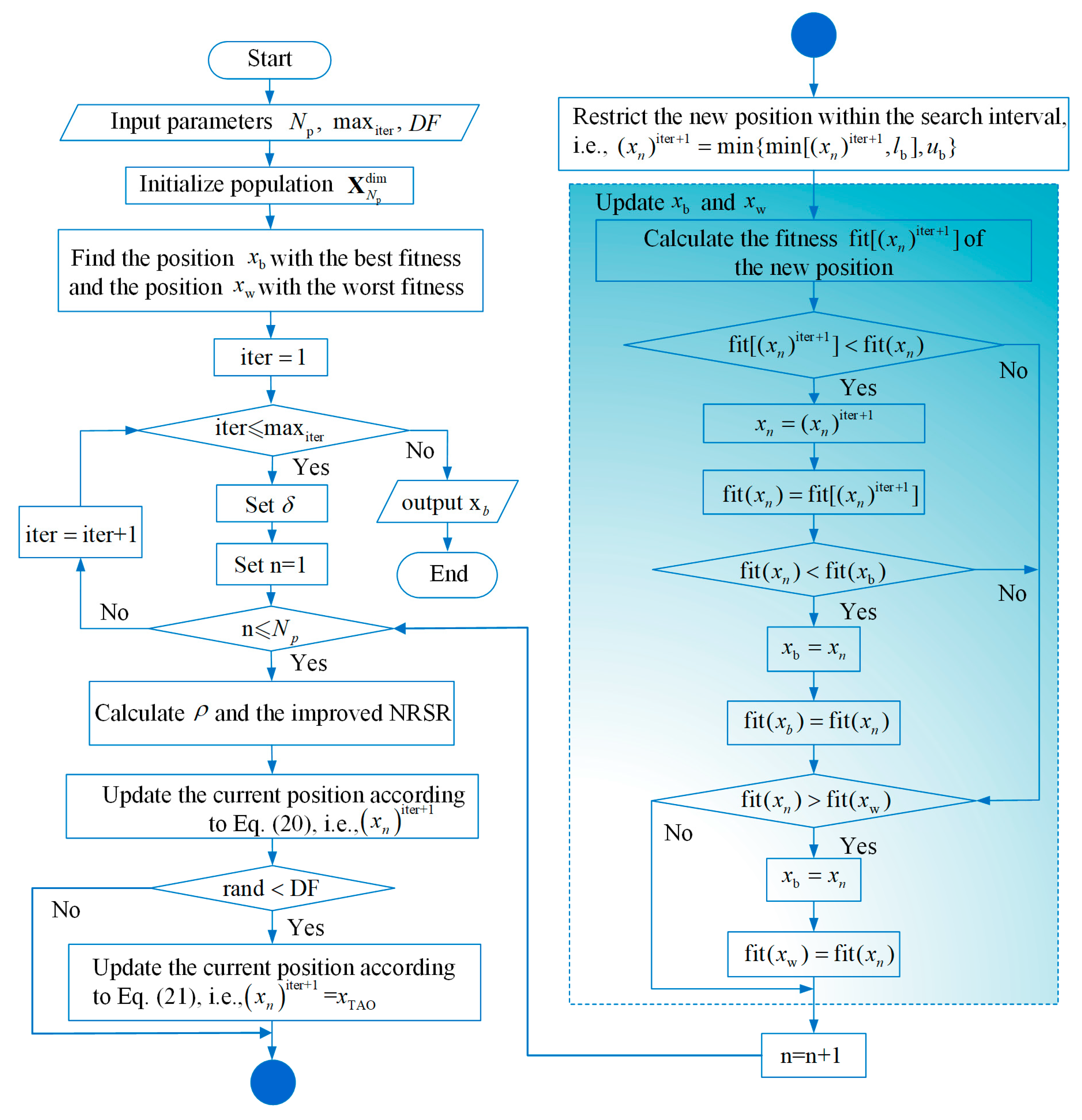
The TAO operation is only introduced when rand < D F . D F is the decision factor for controlling trap avoidance, and its default value is 0.5. The iteration process of the NRBO algorithm is shown in Figure 2.

3. Principle of SHAP Interpretability Method

SHAP is a model interpretation method that explains the prediction results of the BOA-LightGBM model via SHAP values. The SHAP method can decompose the model output into a linear combination of various feature variables, thus quantifying the marginal contribution of each feature to the model output and solving the “black box” problem of traditional machine learning models. The interpretation form of SHAP is expressed as:
y ^ i = ϕ 0 + j ϕ j i
where ϕ 0 is the base value of the model output, and ϕ j i denotes the contribution value of the j -th feature to sample i . The calculation of SHAP values takes all possible feature combinations S into account:
ϕ i = s N i [ S ! M S 1 ! ] · f S U j f S
In this study, the TreeSHAP method is adopted to efficiently calculate SHAP values in the NRBO–LightGBM tree model. At the global level, SHAP can be used for feature importance ranking; at the local level, it can provide prediction explanations for each sample; and at the interaction level, it can reveal the nonlinear interaction effects between features.
The analysis results of SHAP can reveal the specific action mechanism of the key input variable set x i = ( τ c , l s , θ , m I ) on the prediction target y i = ( u 0 , h 0 ) , which helps improve the transparency and interpretability of the prediction model.
In summary, the flowchart of the slope deformation prediction model based on NRBO-LightGBM and its interpretability analysis is shown in Figure 3.

4. Case Study

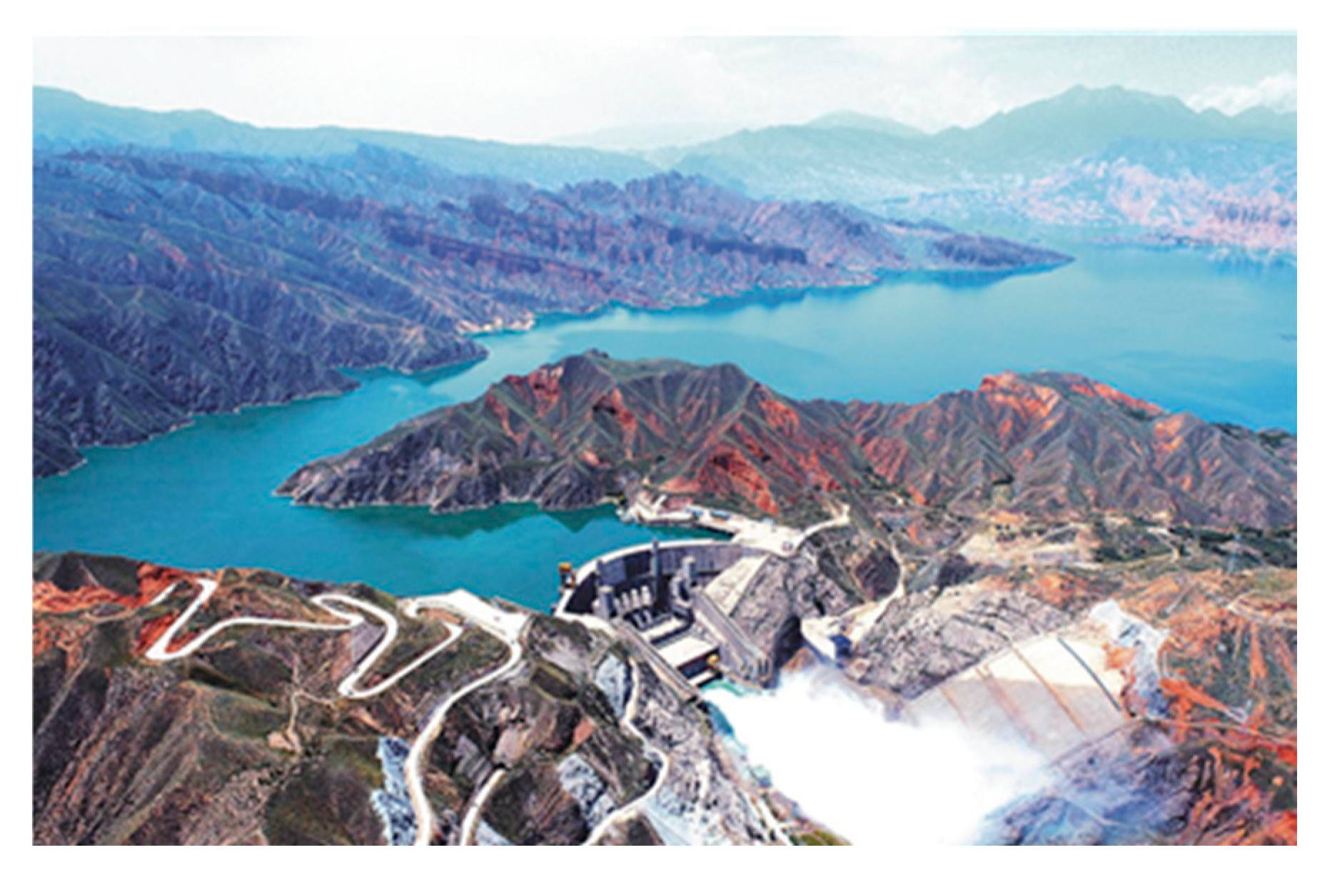
The Lijiaxia Hydropower Station is one of the large cascade hydropower plants on the upper Yellow River, which is located on the main stem of the Yellow River at the boundary between Jianzha County and Hualong County, Qinghai Province, approximately 112 km from Xining, as presented in Figure 4. The project is primarily for power generation, with ancillary benefits such as irrigation. The dam site controls a catchment area of 136,747 km2; the reservoir has a normal pool level of 2180.0 m, a design flood level of 2181.30 m, a total storage capacity of 1.75 × 10⁹ m3, and an installed capacity of 2000 MW.
The water-retaining structure of the Lijiaxia Hydropower Station is a three-center, double-curvature concrete arch dam, divided into 20 monoliths from right to left. On the left bank of the downstream spillway energy-dissipation zone lies the No. III landslide mass. Figure 5a provides an overview of the reservoir corridor, delineating the unstable slope sector on the left bank where deformation has developed. Figure 5b presents a close-up of the No. III-2 landslide mass, showing intensely weathered and fractured rock with local collapses and talus accumulation above the river.

4.1. Datasets

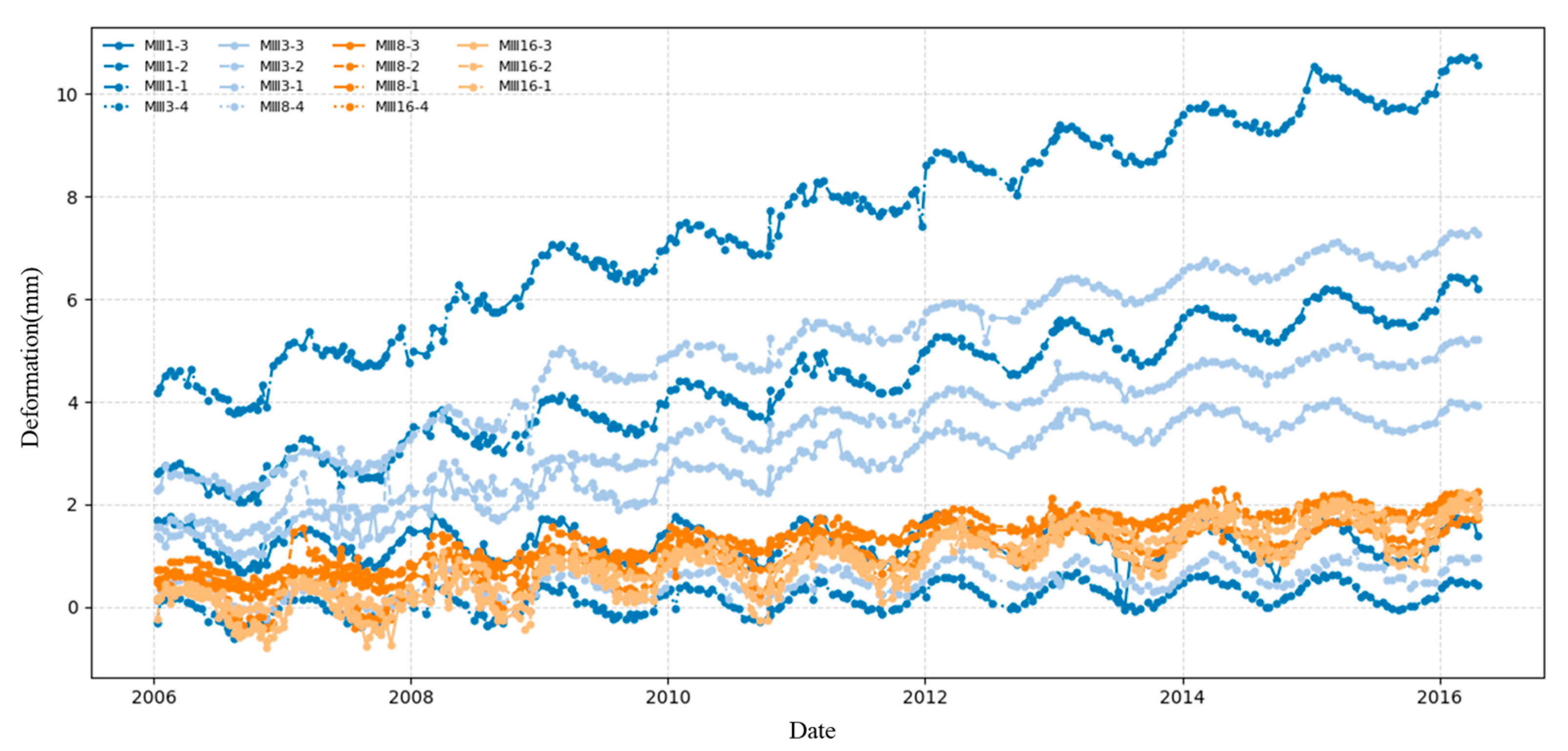
Monitoring for No. III landslide includes 81 surface geodetic survey points, 19 sets of multipoint extensometers (MPBX), GNSS monitoring, and routine visual inspections. Considering data completeness and quality, this study uses the MPBX measurements to develop the monitoring model. At present, four MPBX installations are operating normally, with monitoring initiated on 22 January 2002. Except for site M1, which has three anchors (measurement rods), the other three MPBX installations each have four anchors, and the current monitoring interval is once per month. Due to access hazards along the observation road during certain periods, gaps occur in the monitoring records. Therefore, the analysis period for slope displacement in this study is restricted to 10 January 2006–19 April 2016. Considering instrument reliability and data completeness, we selected monitoring points MIII1-1–MIII1-3, MIII3-1–MIII3-4, MIII8-1–MIII8-4, and MIII16-1–MIII16-4 as the study sites. The monitoring time series for the 15 points are plotted in Figure 6. As shown, deformation in the No. III landslide exhibits a similar variation pattern, a pronounced periodic regular, and several points display a clear increasing trend that warrants continued observation and analysis.

4.2. Results of the Proposed Model and Comprison with Other Models

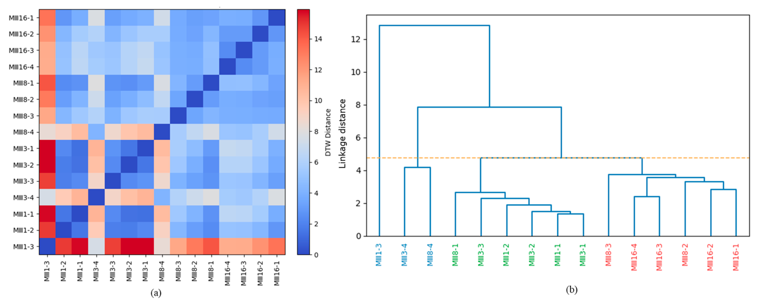
The following calculation and visualization were conducted in the IDLE environment using Python 3.10 (64-bit). Considering the spatial heterogeneity of slope deformation, we classified the deformation data series before modeling according to their temporal patterns, and we jointly modeled sequences in the same group with high similarity. This stratification ensures greater robustness of the prediction models. We herein applied Dynamic Time Warping (DTW) to classify the deformation data series. The results of clustering are presented in Figure 7.
The DTW distance heatmap (a) shows clear block structures, indicating strong within-group similarity and between-group dissimilarity among the slope deformation data series. Cutting the dendrogram (b) at the indicated level yields three clusters: (i) Cluster 1 (MIII1-3, MIII3-4 and MIII8-4), exhibiting highly consistent seasonal patterns; (ii) a moderate-amplitude, relatively stable group centered on Cluster 2 (MIII1-1~MIII1-2, MIII3-1~MIII3-3 and MIII8-1); and (iii) Cluster 3 (MIII16-1~MIII16-4, MIII8-2 and MIII 8-3), showing larger amplitudes and step-like or accelerating behavior. With the examination of the slope deformation process lines shown in Figure 6, it can be found that the clustering results can reflect the coherent spatiotemporal characteristic of the slope deformation data series. Subsequently, informed by the clustering results, the proposed model is constructed separately for each cluster of monitoring data. Here, we use a chronological 80/20 split (training: April 2006–February 2014; testing: February 2014–April 2016) and a rolling-origin scheme to mimic deployment.
Based on the clustering results, the monitoring points were assigned into three groups using DTW clustering method, and we developed a NRBO–LightGBM model for each group. Here, we selected the input variables as H, H 2 , H 3 , H 4 , sin 2 π   j t 365 , cos 2 π   j t 365 , t and ln t , where H is the upstream water level and t is the time. We first calibrated the deformation monitoring data spanning 4 April 2006 to 11 February 2014 to establish the predicting model. Subsequent validation was conducted using reserved test datasets. Figure 8 illustrates the fitting and predicting performance for three representative monitoring points in Group 1 (MIII1-3, MIII3-4 and MIII8-4). Measured deformation data are plotted in black lines, with red, blue, and orange curves corresponding to fitted and predicted results from the NRBO–LightGBM model, LightGBM model, and the stepwise regression model, respectively. The proposed model demonstrates strong agreement with observations across the entire timeline. Extended results for the remaining 12 monitoring points in Groups 2–3 are provided in Appendix A.
Following the development of the prediction model, we systematically evaluated its performance through comparative analysis with three benchmark models: the stepwise regression model and LightGBM model. Three quantitative indicators were employed for performance assessment: the coefficient of determination (R2), root mean square error (RMSE), and mean absolute error (MAE), defined as follows:
R 2 = 1 i = 1 n ( y i y ^ i ) 2 i = 1 n ( y i y ¯ ) 2
R M S E = 1 n i = 1 n ( y i y ^ i ) 2
M A E = 1 n i = 1 n | y i y ^ i |
where y ^ i , y i denotes the series of fitting and measuring data, respectively; y ¯ i is the mean of measuring data series; and n is the number of measuring data points.
The indicators R2, RMSE, and MAE are used to quantify the agreement between measured and fitting values. As shown in Table 2, these metrics were calculated for each monitoring point using the training dataset. The model demonstrates strong fitting capability where R2 exceeds 0.8, a threshold comfortably surpassed by all monitoring points (the range of R2: 0.8511–0.9903). Residual analysis revealed values of s spanning 0.0998 to 0.1992, further validating the model’s fitting performance.
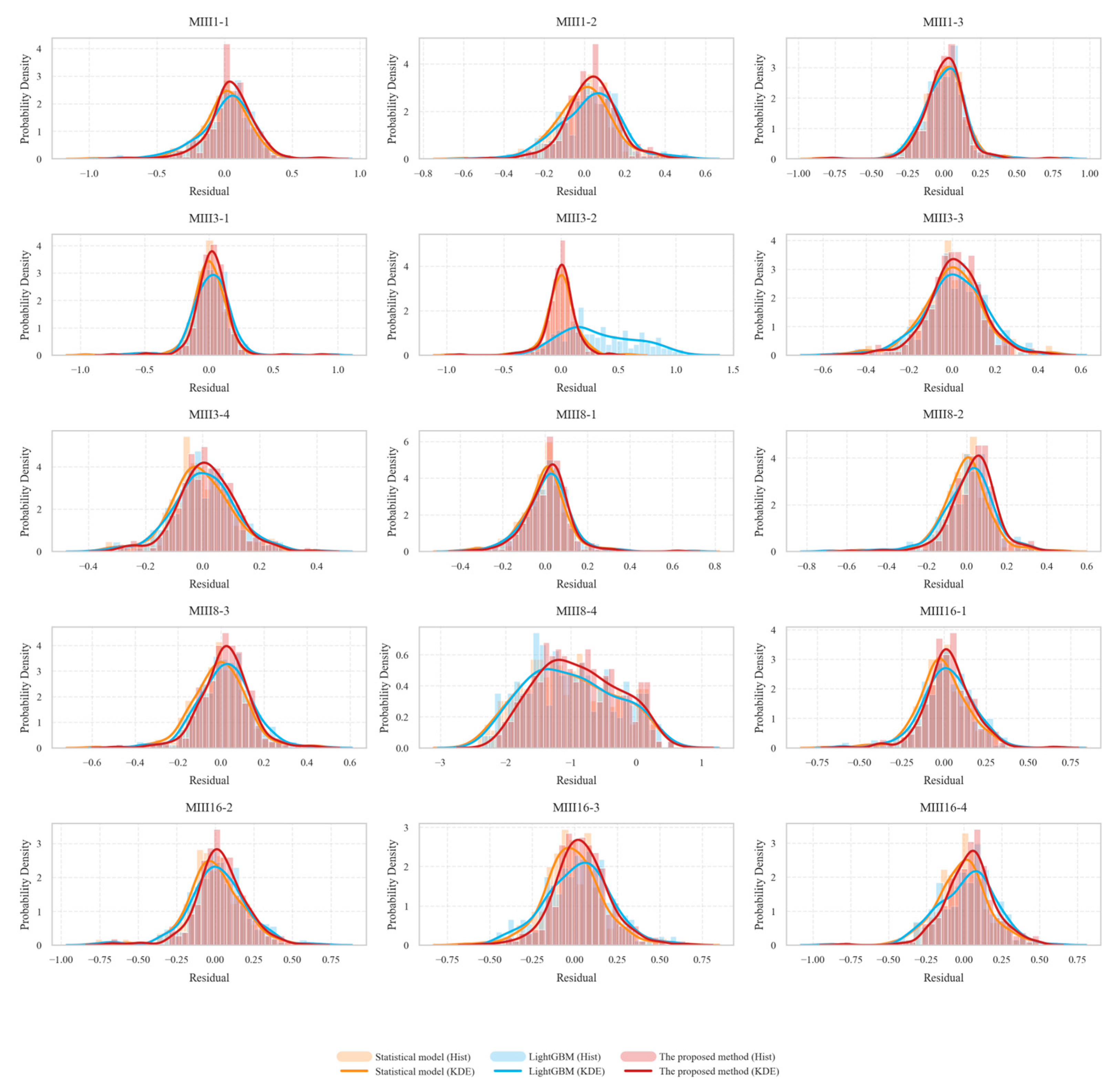
Figure 9 presents the residual probability density distributions of the predicted and measured slope deformation for 15 monitoring points using different models. Overall, the residuals obtained by the proposed NRBO–LightGBM model (green) exhibit a more centralized and symmetrical distribution around zero compared with those of the traditional statistical model (yellow) and the standard LightGBM model (blue). This indicates that the proposed method effectively reduces both systematic and random errors in the slope deformation prediction process. Furthermore, the narrower spread of residuals in the proposed model demonstrates its superior prediction stability and generalization capability across multiple monitoring locations. In contrast, the traditional statistical model shows higher kurtosis and heavier tails, implying larger deviations and lower reliability in displacement prediction.
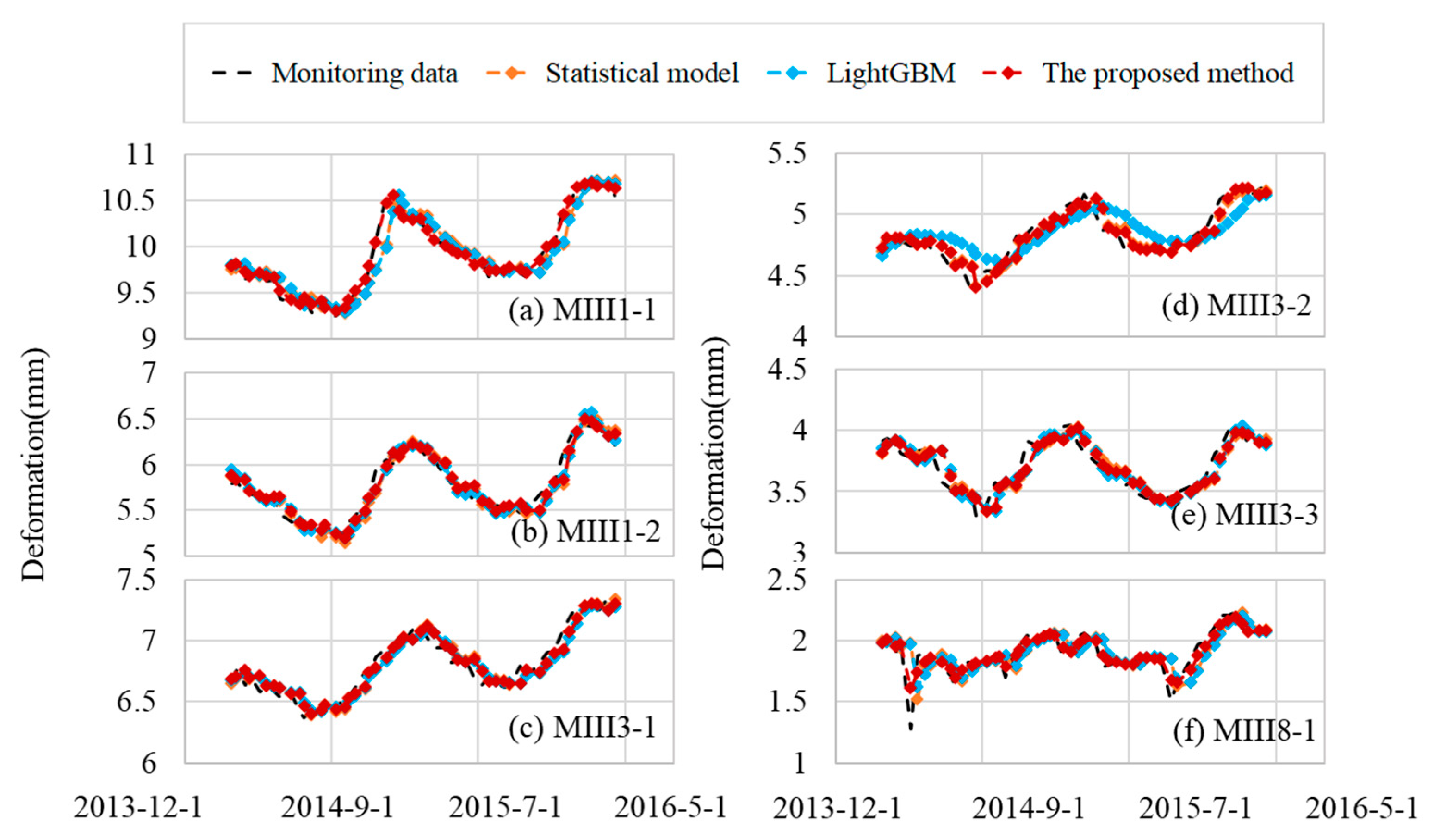
Figure 10 presents the time series of observed and predicted deformations for representative monitoring points in Cluster 1 (MIII3-3, MIII3-4, and MIII8-4). It can be indicated that the deformation predicted by the proposed NRBO–LightGBM model (red dashed line) shows the highest consistency with the measured monitoring data (black dashed line), accurately capturing both the long-term deformation trend and the short-term fluctuation characteristics. Compared with the traditional statistical model (yellow dashed line) and the standard LightGBM model (blue dashed line), the proposed method exhibits smaller deviations and better phase alignment with the actual measurements, particularly during deformation reversal periods and peak stages. This indicates that the proposed model effectively improves temporal fitting capability and generalization performance, enabling more robust and accurate deformation prediction of slope displacement behavior.
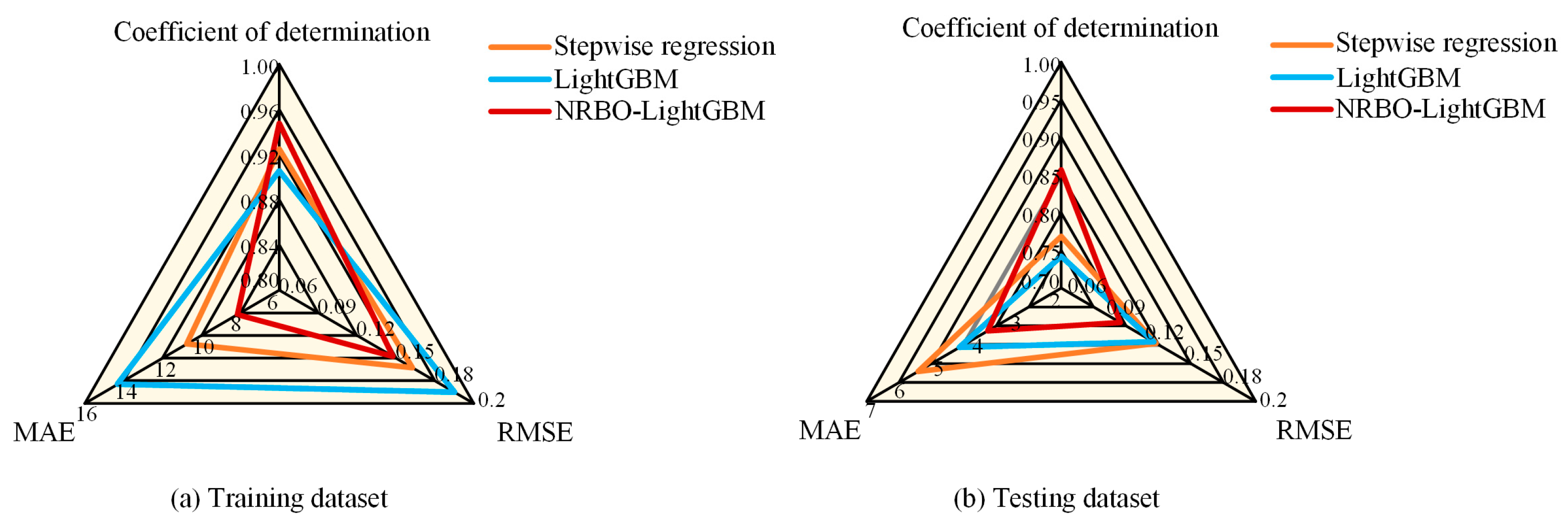
To quantitatively evaluate the performance of different models, Figure 11 illustrates the comparative results of three models—stepwise regression, LightGBM, and the proposed NRBO–LightGBM based on the evaluation indicators of average R2, RMSE, and MAE for both the training and testing datasets of 15 monitoring points. As shown in the radar plots, the proposed NRBO–LightGBM model achieves the highest average R2 (0.9476 for fitting and 0.8569 for predicting) values of 15 monitoring points and the lowest average RMSE (0.1377 for fitting and 0.0955 for predicting) and MAE (8.153 for fitting and 3.889 for predicting) in both datasets, indicating superior fitting accuracy and generalization performance. Compared with the conventional stepwise regression model, NRBO–LightGBM exhibits a significantly enhanced capability in capturing nonlinear relationships within the deformation data. Furthermore, the improvement over the standard LightGBM model demonstrates the effectiveness of the Newton–Raphson-based optimizer in tuning hyperparameters, which enables better model stability and predictive robustness. These results confirm that the proposed optimization-enhanced model provides a more reliable and precise framework for slope deformation prediction under complex environmental influences. For completeness, Table 3 lists the corresponding average R2, RMSE, and MAE of 15 monitoring points, which are consistent with the trends in Figure 11.

4.3. Shap Analysis

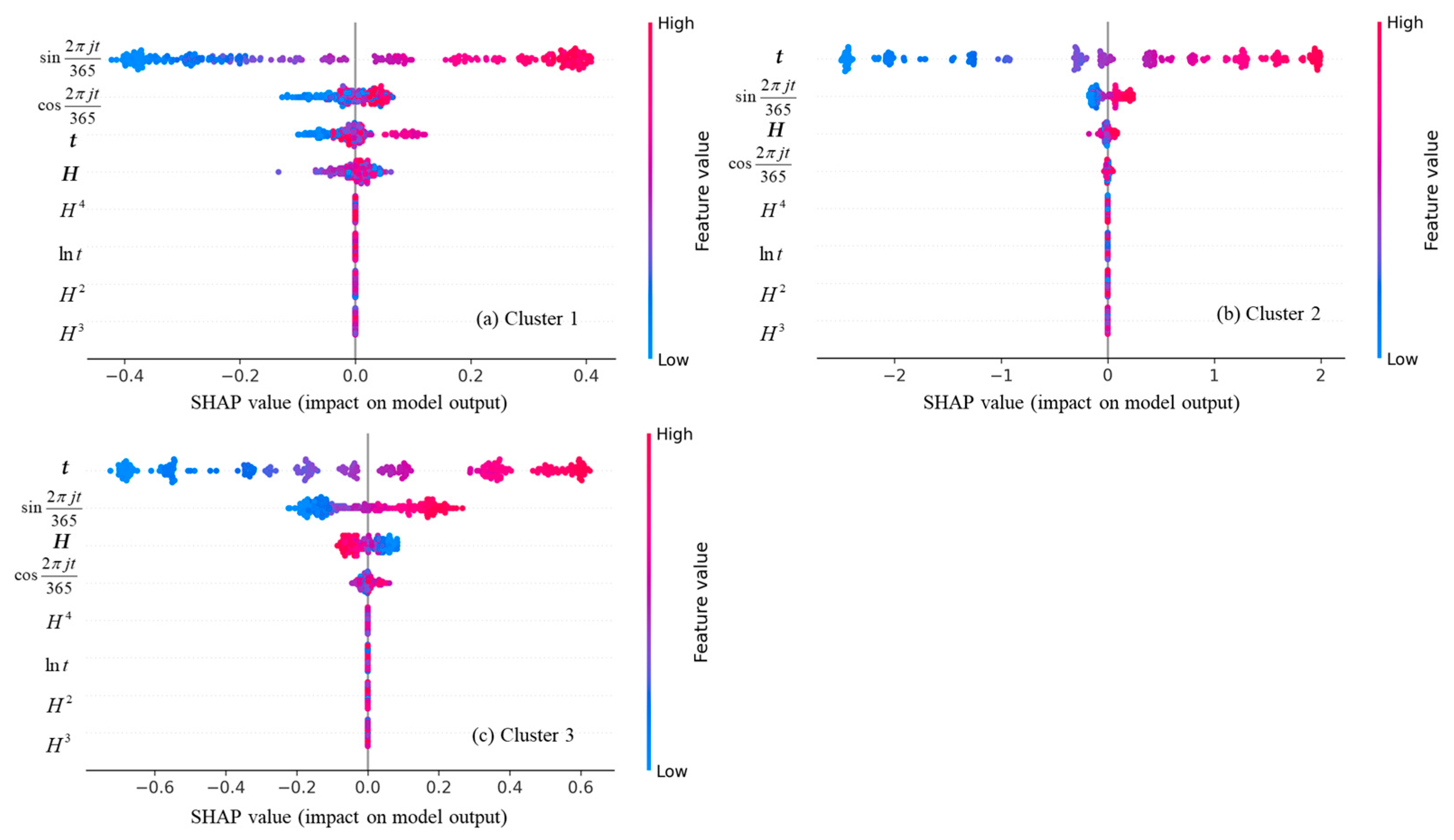
To further interpret the internal mechanism and feature contribution of the developed deformation prediction model, SHAP (Shapley additive explanations) analysis was employed. SHAP provides a unified framework to quantify the marginal effect of each input variable on the model output, thereby enabling the identification of key driving factors controlling slope deformation. Compared with traditional sensitivity analysis, SHAP not only measures the global importance of variables but also explains their local influence on individual predictions, offering a transparent and physically interpretable insight into the data-driven model behavior. In this study, the SHAP approach was applied to evaluate the influence of hydrological and temporal variables (e.g., H, H 2 , H 3 , H 4 , sin 2 π   j t 365 , cos 2 π   j t 365 , t, and ln t ) on the predicted slope deformation. Figure 12 exhibits the distribution of SHAP values for each input variables.
As illustrated in the SHAP summary plot, the contribution of different input variables to the model output across the three identified clusters exhibits significant variability. For Cluster 1 and Cluster 3, the time variable t shows the largest range of SHAP values, indicating that temporal evolution exerts a dominant influence on the deformation prediction. The sinusoidal terms sin(2πjt/365) and cos(2πjt/365) also have a noticeable, though smaller, contribution, implying the presence of a seasonal or cyclic deformation pattern. In contrast, the SHAP values associated with the water level H and its higher-order terms ( H 2 , H 3 , H 4 ) are close to zero, suggesting that short-term water level fluctuations have a relatively limited marginal impact on the overall deformation response within the analyzed period. In Cluster 2, the time variable t and its harmonic terms exhibit the largest SHAP contributions, revealing that deformation is mainly governed by long-term temporal evolution and seasonal cycles rather than instantaneous water-level changes.
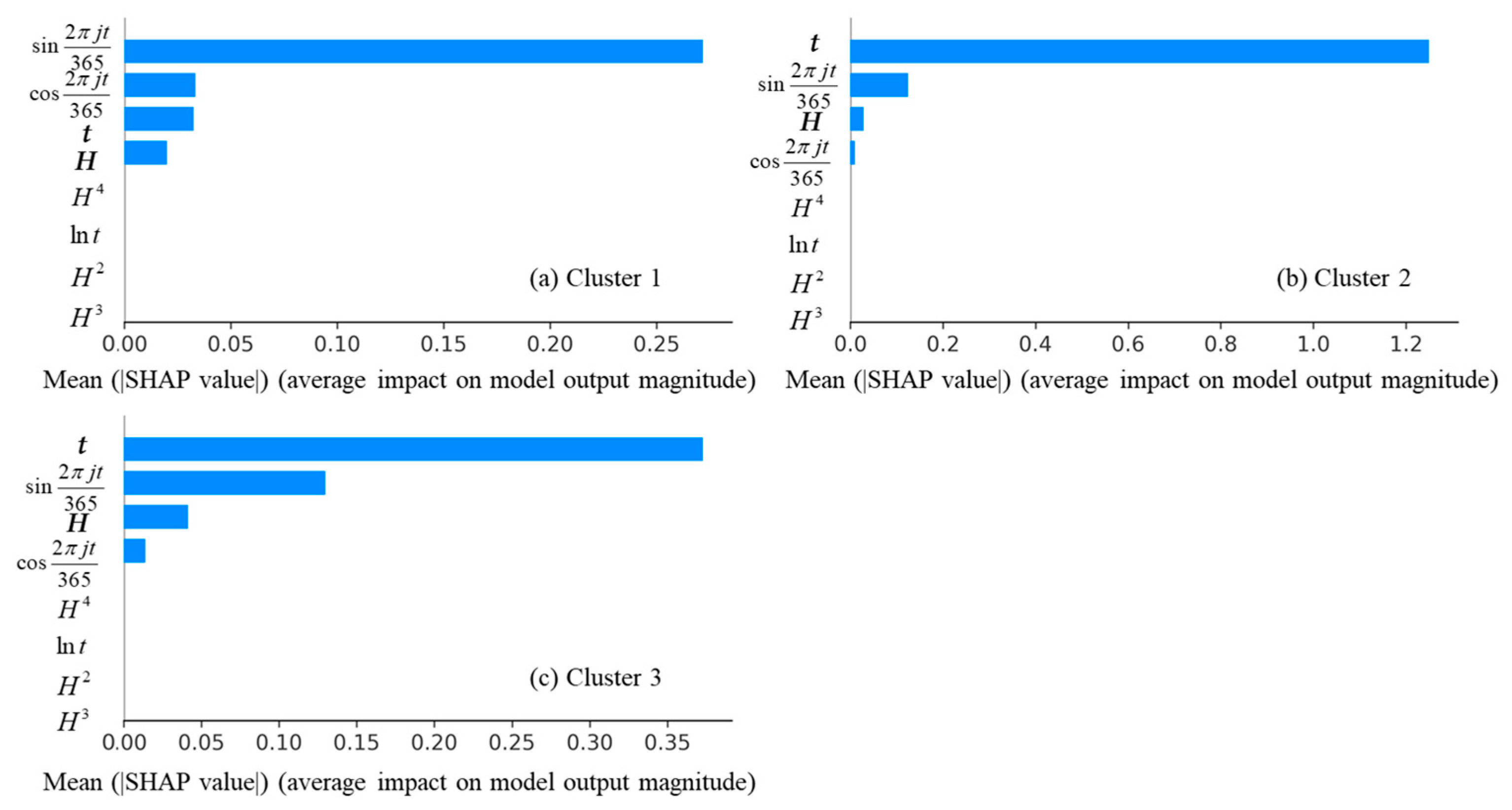
The mean absolute SHAP values plots as shown in Figure 13 further quantify these differences in feature importance. Specifically, the average SHAP magnitudes demonstrate that hydrological factors dominate in Cluster 1, temporal evolution is the major driver in Cluster 2, and Cluster 3 exhibits a transitional pattern between the two extremes. These findings not only validate the clustering results but also offer physical interpretability of the data-driven model, linking predicted deformation patterns with their underlying mechanisms. Such interpretability enhances the credibility of the proposed framework and provides practical insight for targeted monitoring and early-warning strategies in reservoir-induced landslides.

4.4. Limitations and Future Work

The proposed NRBO–LightGBM–SHAP framework demonstrates high predictive accuracy and provides interpretable insights into model behavior, exhibiting promise for applications in engineering operation and management. However, the framework remains constrained by data quality: gaps, noise, and sensor drift may materially degrade both predictive performance and SHAP-based interpretability. Furthermore, the site-specific validation (single-reservoir case) limits the generalizability of the results without additional re-training and local calibration. Future research will focus on enhancing data quality assurance and control through robust filtering, gap interpolation, and sensor cross-validation, as well as on conducting multi-site external validation across diverse hydrogeological and operational regimes. The modeling framework will be further enriched by integrating physics-informed features (e.g., effective stress and infiltration proxies, pore-pressure monitoring) and implementing calibrated uncertainty quantification approaches (such as quantile regression, NGBoost, and conformal prediction) to provide actionable thresholds with credible confidence intervals. To improve robustness under changing conditions, future work will also explore online and continual learning strategies, rolling-origin evaluation schemes, and hybrid physics–machine learning as well as spatiotemporal graph-based models while maintaining interpretability through grouped or interaction-level SHAP analyses.

5. Conclusions

The proposed framework, which integrates the NRBO optimization algorithm and LightGBM model, offers several advantages for reservoir-slope deformation prediction. Primarily, slope deformation monitoring points are classified by their time-series, thereby reflecting the temporal evolution of deformation. This improves the reliability of monitoring-point partitioning and yields a more realistic representation of slope behavior. Then, the Newton–Raphson-based optimizer (NRBO) effectively addresses the hyperparameter sensitivity of tree-boosting models, enhancing adaptability and robustness and leading to more accurate and stable predictions. Third, through the SHAP interpretability analysis, the internal mechanism of the model can be effectively elucidated. The results indicate that the temporal evolution represented by the time variable t is the predominant factor influencing slope deformation. Comparative experiments on monitoring data of slope deformation confirm that the proposed framework surpasses traditional statistical models and untuned LightGBM in both predictive accuracy and interpretability.
Despite these strengths, several limitations should be noted. The method requires sufficient and continuous monitoring data for both clustering and model training, which may constrain applicability where records are short or irregular. While the clustering step improves group coherence, its performance can degrade with sparse networks or strong nonstationarities. Moreover, although SHAP enhances interpretability, the approach remains predominantly data-driven; thus, causal attribution is indirect compared with fully physics-based models, and the identified thresholds may be site-specific.
Future research can mitigate these limitations in two ways: (i) Develop hybrid schemes that couple data-driven LightGBM with physics-informed constraints (e.g., pore-pressure response or simplified stability indices) to improve both accuracy and causal interpretability; (ii) Introduce more scalable partitioning and dimensionality-reduction techniques to handle large monitoring networks and long time series, and incorporate online learning for real-time updating.

Author Contributions

Conceptualization, J.C., J.S., and C.S.; methodology, J.C. and Y.X.; software, F.X. and C.L.; validation, X.L.; formal analysis, C.L. and J.C.; investigation, J.C. and Y.H.; resources, C.S.; data curation, C.L. and J.C.; writing—original draft preparation, J.C., J.S. and Y.X.; writing—review and editing, J.C. and C.S.; supervision, C.S.; funding acquisition, C.S. and Y.H. All authors have read and agreed to the published version of the manuscript.

Funding

This study was supported by the National Natural Science Foundation of China (Nos. 52209159, 52469022), the Fundamental Research Funds for the Central Universities (Grant No. B250201005), the Jiangxi Provincial Natural Science Foundation (Nos. 20242BAB20239, 20252BAC240690), and the Science and Technology Projects of the Jiangxi Provincial Department of Water Resources, China (Nos. 202425YBKT24, 202425YBKT27, 202527ZDKT25), the Jiangsu young science and technological talents support project (JSTJ-2024-185).

Data Availability Statement

The dataset will be made available upon request from the authors.

Conflicts of Interest

The authors declare no conflicts of interest.

Appendix A. Fitting and Predicting Results of Other Monitoring Points

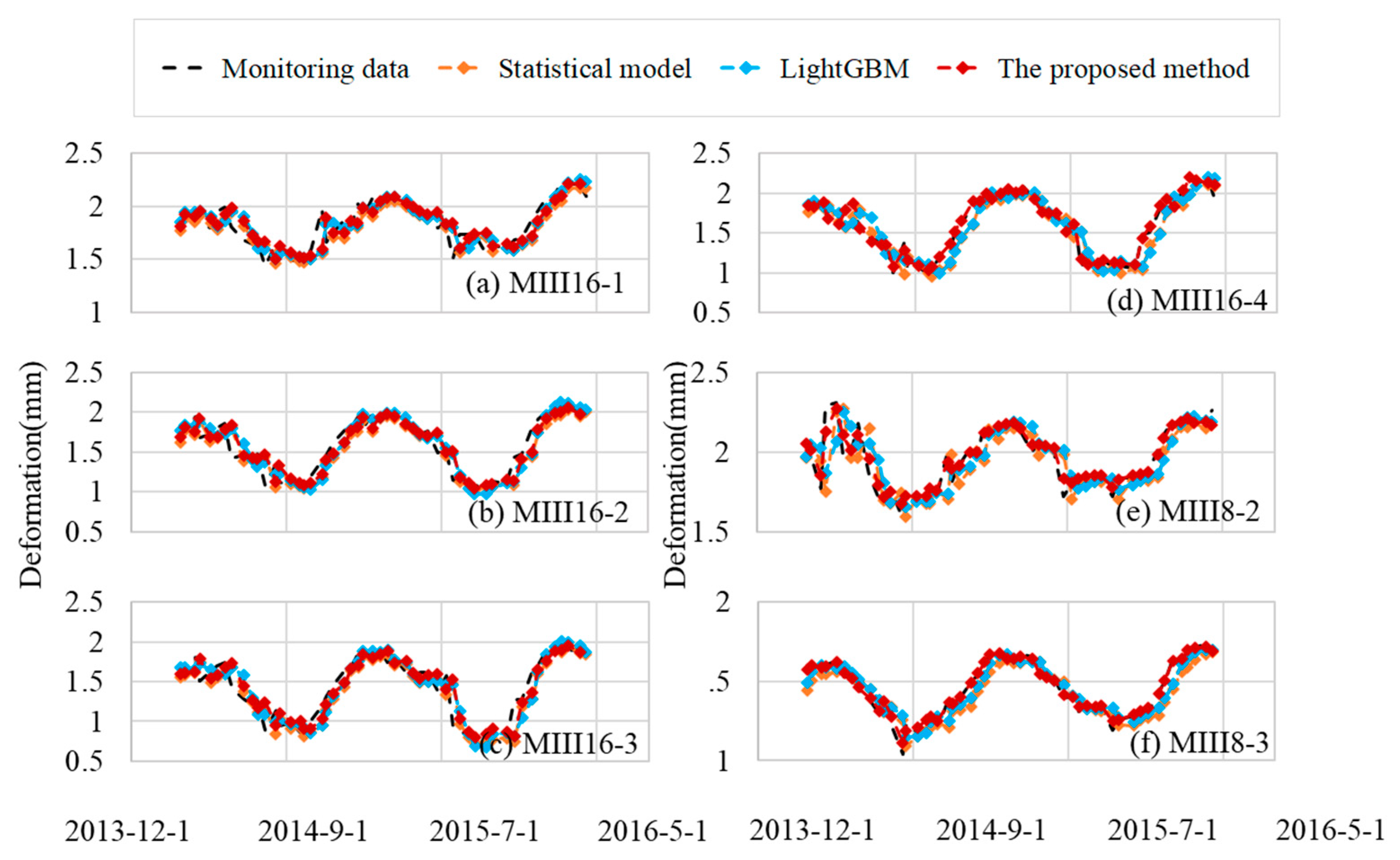
Figure A1 and Figure A2 illustrate the process lines of fitting and predicting deformation for Cluster 2 and Cluster 3, respectively.
Figure A1. Fitting and predicting results of monitoring points in Cluster 2 for reservoir slope deformation under different models.
Water 17 03248 g0a1
Figure A2. Fitting and predicting results of monitoring points in Cluster 3 for reservoir slope deformation under different models.
Water 17 03248 g0a2

Appendix B. Fitting and Predicting Results of Other Monitoring Points

Figure A3 and Figure A4 illustrate the process lines of reservoir slope deformation in the testing dataset for Cluster 2 and Cluster 3, respectively.
Figure A3. Predicting results of monitoring points in Cluster 2 for reservoir slope deformation under different models.
Water 17 03248 g0a3
Figure A4. Predicting results of monitoring points in Cluster 3 for reservoir slope deformation under different models.
Water 17 03248 g0a4

Appendix C. Pseudocode of the NRBO–LightGBM–SHAP Framework

Algorithm A1. Pseudocode of the proposed framework.
Input: Monitoring dataset D = {(Xt, yt)} at N monitoring points
Output: Predicted deformation ŷt and SHAP-based feature attributions

1: Data Preprocessing
2:  Handle missing values, normalize features, and align time indices.
3:  Construct physics-informed and memory features (e.g., rainfall, reservoir level, lagged deformation).

4: Response-Coherent Clustering
5:  Cluster deformation series into response-coherent groups using similarity in temporal patterns.
6:  For each cluster, initialize LightGBM parameters θ0.

7: NRBO-Based Hyperparameter Optimization
8:  For each cluster c do
9:   Initialize iteration k = 0.
10:   Repeat until convergence
11:    Compute gradient: gk = ∂L/∂θk.
12:    Compute Hessian: Hk = ∂2L/∂θk2.
13:    Update parameters: θk+1 = θk − α·Hk−1·gk,
      where α is a damping coefficient controlled by line search.

14:   End Repeat
15:  Obtain optimized parameters θ*.

16: Model Training and Validation
17:  Train LightGBM using optimized θ* on the training dataset.
18:  Evaluate model on the testing dataset to compute R2, RMSE, and MAE.

19: SHAP-Based Interpretation
20:  Compute SHAP values for all input features.
21:  Aggregate global and local attributions.
22:  Generate feature-importance and partial-dependence plots.

23: Output
24:  Predicted deformation series ŷt.
25:  SHAP-based feature attributions and derived warning thresholds.

References

  1. Huo, T.; He, Y.; Liu, Y.; Yang, W.; Zhang, L.; Chen, H.; Fang, Y.; Gao, B.; Zhang, X. InSAR-Based Surface Deformation Analysis and Trend Prediction in Permafrost Areas Along the Qinghai-Tibet Railway Using Sentinel-1A and Environmental Factors. IEEE J. Sel. Top. Appl. Earth Obs. Remote Sens. 2025, 18, 9297–9320. [Google Scholar] [CrossRef]
  2. Wang, L.; Wang, L.; Zhang, W.; Meng, X.; Liu, S.; Zhu, C. Time Series Prediction of Reservoir Bank Landslide Failure Probability Considering the Spatial Variability of Soil Properties. J. Rock Mech. Geotech. Eng. 2024, 16, 3951–3960. [Google Scholar] [CrossRef]
  3. Yin, Y.; Wang, L.; Zhang, W.; Zhang, Z.; Dai, Z. Research on the Collapse Process of a Thick-Layer Dangerous Rock on the Reservoir Bank. Bull. Eng. Geol. Environ. 2022, 81, 109. [Google Scholar] [CrossRef]
  4. Li, Y.; Zhang, W.; Zhang, K.; Gou, Q.; Tang, S.; Guo, F. Study on Slope Deformation Partition and Monitoring Point Optimization Considering Spatial Correlation. Nat. Hazards 2024, 120, 13109–13136. [Google Scholar] [CrossRef]
  5. Song, K.; Yang, H.; Liang, D.; Chen, L.; Jaboyedoff, M. Step-Like Displacement Prediction and Failure Mechanism Analysis of Slow-Moving Reservoir Landslide. J. Hydrol. 2024, 628, 130588. [Google Scholar] [CrossRef]
  6. Dong, M.; Wu, H.; Hu, H.; Azzam, R.; Zhang, L.; Zheng, Z.; Gong, X. Deformation Prediction of Unstable Slopes Based on Real-Time Monitoring and DeepAR Model. Sensors 2021, 21, 14. [Google Scholar] [CrossRef] [PubMed]
  7. Du, S.; Feng, G.; Wang, J.; Feng, S.; Malekian, R.; Li, Z. A New Machine-Learning Prediction Model for Slope Deformation of an Open-Pit Mine: An Evaluation of Field Data. Energies 2019, 12, 1288. [Google Scholar] [CrossRef]
  8. Chen, L.; Wu, B.B.; Liu, J.Y. Stepwise Regression Arithmetic and Its Application on Slope Safety Monitoring. Appl. Mech. Mater. 2012, 204–208, 2859–2864. [Google Scholar] [CrossRef]
  9. Li, J.; Meng, Z.; Zhang, J.; Chen, Y.; Yao, J.; Li, X.; Qin, P.; Liu, X.; Cheng, C. PPrediction of Seawater Intrusion Run-Up Distance Based on K-Means Clustering and ANN Model. J. Mar. Sci. Eng. 2025, 13, 377. [Google Scholar] [CrossRef]
  10. Zuan, P.; Huang, Y. Prediction of Sliding Slope Displacement Based on Intelligent Algorithm. Wirel. Pers. Commun. 2018, 102, 3141–3157. [Google Scholar] [CrossRef]
  11. Li, L.; Qiang, Y.; Li, S.; Yang, Z. Research on Slope Deformation Prediction Based on Fractional-Order Calculus Gray Model. Adv. Civ. Eng. 2018, 2018, 9526216. [Google Scholar] [CrossRef]
  12. Wu, H.; Dong, Y.; Shi, W.; Clarke, K.C.; Miao, Z.; Zhang, J.; Chen, X. An Improved Fractal Prediction Model for Forecasting Mine Slope Deformation Using GM (1,1). Struct. Health Monit. 2015, 14, 502–512. [Google Scholar] [CrossRef]
  13. Du, S.W.; Li, Y. A Novel Deformation Forecasting Method Utilizing Comprehensive Observation Data. Adv. Mech. Eng. 2018, 10, 1687814018796330. [Google Scholar] [CrossRef]
  14. Du, S.; Song, R.; Qu, Q.; Zhao, Z.; Sun, H.; Chen, Y. Surface Deformation Prediction Model of High and Steep Open-Pit Slope Based on APSO and TWSVM. Elektronika ir Elektrotechnika 2024, 30, 77–83. [Google Scholar] [CrossRef]
  15. Mohammady, M.; Pourghasemi, H.R.; Amiri, M. Land Subsidence Susceptibility Assessment Using Random Forest Machine Learning Algorithm. Environ. Earth Sci. 2019, 78, 503. [Google Scholar] [CrossRef]
  16. Zang, H.H.; Li, D.Q.; Tang, X.S.; Rong, G. Machine Learning for Time Series Prediction of Valley Deformation Induced by Impoundment for High Arch Dams. Bull. Eng. Geol. Environ. 2025, 84, 194. [Google Scholar] [CrossRef]
  17. Yu, M.; Chen, L.; Fan, X.; Ma, P.; Zhao, S.; Wu, Z.; Yang, F.; Xu, L.; Shan, M.; Xie, X.; et al. Validating and Enhancing Data-Driven Landslide Susceptibility Prediction by Model Explanation and MT-InSAR Techniques. Int. J. Digit. Earth 2025, 18, 2509857. [Google Scholar]
  18. Hu, J.; Li, X. A Novel Prediction Model Construction and Result Interpretation Method for Slope Deformation of Deep Excavated Expansive Soil Canals. Expert Syst. Appl. 2024, 236, 121326. [Google Scholar] [CrossRef]
  19. Zhou, X.; He, Y.; Zhang, W.; Liu, D. Multifractal Characteristics and Displacement Prediction of Deformation on Tunnel Portal Slope of Shallow-Buried Tunnel Adjacent to Important Structures. Buildings 2024, 14, 1662. [Google Scholar] [CrossRef]
  20. Wang, S.; Lyu, T.L.; Luo, N.; Chang, P. Deformation Prediction of Rock Cut Slope Based on Long Short-Term Memory Neural Network. Int. J. Mach. Learn. Cybern. 2024, 15, 795–805. [Google Scholar] [CrossRef]
  21. Xi, N.; Yang, Q.; Sun, Y.; Mei, G. Machine Learning Approaches for Slope Deformation Prediction Based on Monitored Time-Series Displacement Data: A Comparative Investigation. Appl. Sci. 2023, 13, 4677. [Google Scholar] [CrossRef]
  22. Wang, Y.; Li, S.; Li, B. Deformation Prediction of Cihaxia Landslide Using InSAR and Deep Learning. Water 2022, 14, 3990. [Google Scholar] [CrossRef]
  23. Özsen, H.; Kaygusuz, B. Experimental Analysis of Various Deep Learning Methods for Predicting Displacements in an Open-Pit Coal Mine. Nat. Hazards 2025, 121, 20629–20654. [Google Scholar] [CrossRef]
  24. Ma, W.; Dong, J.; Wei, Z.; Peng, L.; Wu, Q.; Chen, C.; Wu, Y.; Xie, F. Landslide Displacement Prediction with Gated Recurrent Unit and Spatial–Temporal Correlation. Front. Earth Sci. 2022, 10, 950723. [Google Scholar] [CrossRef]
  25. Deng, Z.X.; Xie, K.; Su, Q.; Xu, L.R.; Hao, Z.R.; Xiao, X.P. Three-Level Evaluation Method of Cumulative Slope Deformation Hybrid Machine-Learning Models and Interpretability Analysis. Constr. Build. Mater. 2023, 408, 133821. [Google Scholar] [CrossRef]
  26. Meng, Z.; Hu, Y.; Jiang, S.; Zheng, S.; Zhang, J.; Yuan, Z.; Yao, S. Slope Deformation Prediction Combining Particle Swarm Optimization-Based Fractional-Order Grey Model and K-Means Clustering. Fractal Fract. 2025, 9, 210. [Google Scholar] [CrossRef]
  27. Dong, Y.F.; Yang, J.; Qin, Y.Y. Prediction of Optimal Design Parameters for Reinforced Soil Embankments with Wrapped Faces Using a GA-BP Neural Network. Appl. Sci. 2024, 14, 6910. [Google Scholar]
  28. Hou, T.K.; Zhou, Z.H.; Zhang, Y.G.; Zhang, J. A Novel Inversion Method of Slope Rock Mechanical Parameters Using Differential Evolution Gray Wolf Algorithm to Optimize Support Vector Regression. Front. Earth Sci. 2025, 13, 1575194. [Google Scholar] [CrossRef]
  29. Gao, J.C.; Nait Amar, M.; Motahari, M.R.; Hasanipanah, M.; Armaghani, D.J. Two Novel Combined Systems for Predicting the Peak Shear Strength Using RBFNN and Meta-Heuristic Computing Paradigms. Eng. Comput. 2022, 38, 129–140. [Google Scholar] [CrossRef]
  30. Bai, H.; Wang, F.; Wang, W.B. Predictive Models for Earthquake-Induced Landslides: Machine Learning Based on Real Case Histories. Environ. Earth Sci. 2025, 84, 477. [Google Scholar] [CrossRef]
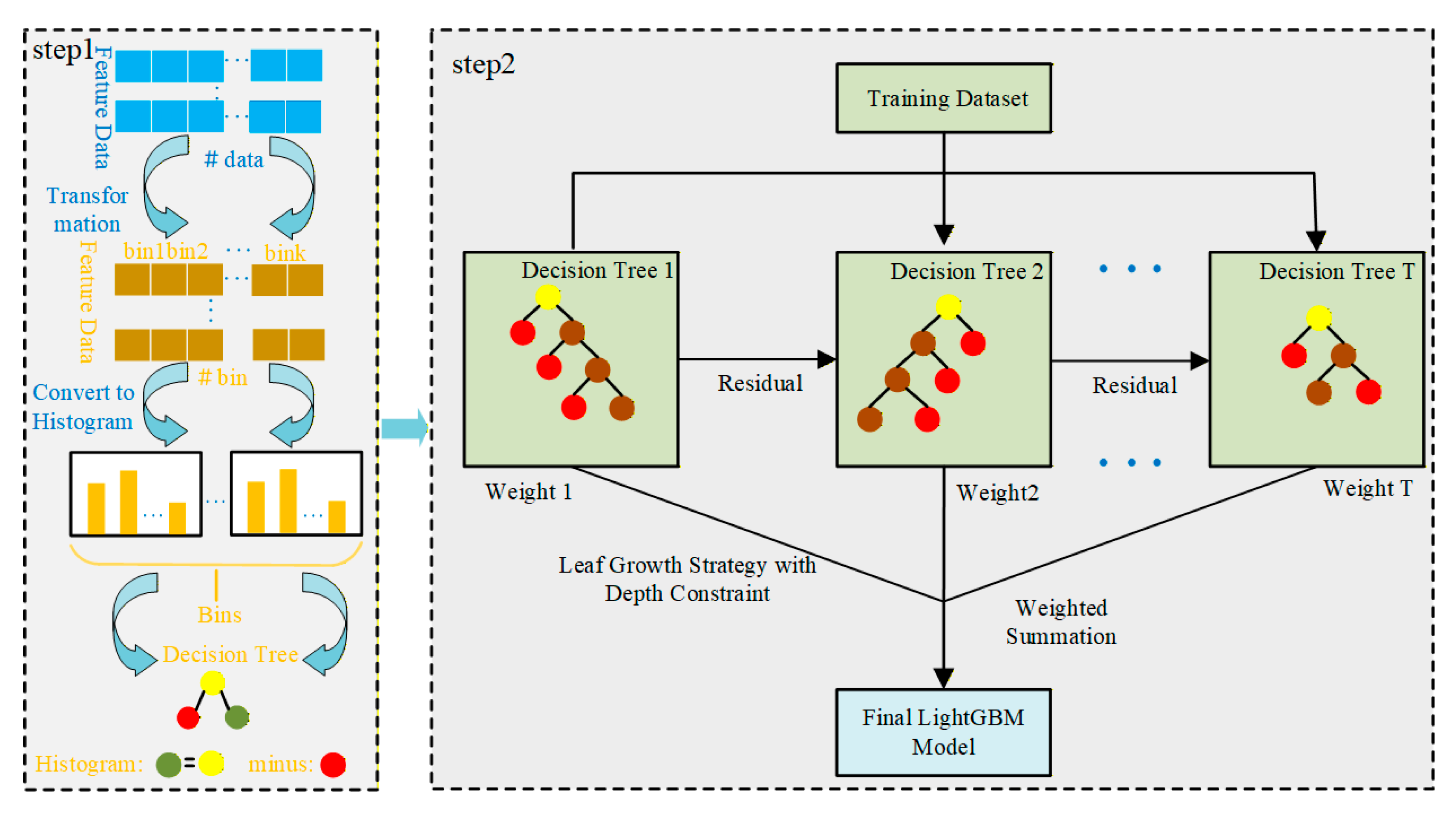
Figure 1. LightGBM model structure diagram.
Water 17 03248 g001
Figure 2. NRBO algorithm flowchart.
Water 17 03248 g002
Figure 3. NRBO–LightGBM slope deformation prediction model and SHAP analysis.
Water 17 03248 g003
Figure 4. Engineering overview of Lijiaxia hydropower station.
Water 17 03248 g004
Figure 5. Collapse condition of the No. III landslides. (a) Collapse condition of the No. III-2 landslide mass. (b) Local collapse of the deformation body of the No. III-2 landslide mass.
Water 17 03248 g005
Figure 6. Collapse condition of the No. III landslides.
Water 17 03248 g006
Figure 7. Clustering results of different deformation data series based on DTW distances: (a) DTW distance matrix of multi-point deformation series; (b) hierarchical clustering dendrogram based on DTW distance.
Water 17 03248 g007
Figure 8. Fitting and predicting results of monitoring points in Cluster 1 for reservoir slope deformation under different models.
Water 17 03248 g008
Figure 9. Residual probability density distributions of monitoring points for reservoir slope deformation under different models.
Water 17 03248 g009
Figure 10. Predicting results of monitoring points in Cluster 1 for reservoir slope deformation under different models.
Water 17 03248 g010
Figure 11. Results of three evaluation indicators for fitting and predicting performance of different models.
Water 17 03248 g011
Figure 12. SHAP summary plot of the distribution of SHAP values for each input variable in different clusters.
Water 17 03248 g012
Figure 13. SHAP summary and mean absolute SHAP value plots showing feature contributions to slope deformation prediction.
Water 17 03248 g013
Table 1. Typical strengths and limitations of related methods.
Method FamilyRepresentative ModelsTypical StrengthsTypical Limitations in Reservoir-Slope Forecasting
Mechanics-informed decompositionsHydraulic–seasonal–aging models; polynomial/d-lag, harmonicPhysically interpretable; parsimonious; easy to calibrateStruggle with step-like kinematics, nonstationary, missing data, nonlinear interactions
Classical ML SVM, RF, GBDT/LightGBM Handles heterogeneity; good tabular performance; modest data requirementSensitive to hyperparameters; limited intrinsic interpretability; often site-wise calibration
Deep/sequence modelsRNN/LSTM/GRU, CNN–RNN hybridsCapture temporal dependence; flexible nonlinear mappingHarder to interpret; prone to overfit; less robust to regime shifts/data gaps
Hybrid physics–MLPhysics-guided features + MLLeverage domain constraints; improved extrapolationAdded feature engineering; require tuning and validation
Optimization metaheuristicsPSO, GA, GWO/WOA/ACODerivative-free; broad applicability; easy to implementSample-inefficient; slow convergence; high variance in optima
Proposed methodNRBO–LightGBMSecond-order, fast convergence; strong tabular accuracy; transparent attributions; supports thresholdingDependent on data quality
Table 2. Indicators of R2, RMSE, and MAE of each monitoring point.
Monitoring PointR2 (/)RMSE (mm)MAE (/)
Cluster 1MIII1-30.85110.136710.8804
Cluster 2MIII1-20.95240.13773.6094
Cluster 2MIII1-10.98320.19922.8156
Cluster 1MIII3-40.85710.099816.5742
Cluster 2MIII3-30.9710.13615.8268
Cluster 2MIII3-20.98230.13384.0285
Cluster 2MIII3-10.97340.14332.8511
Cluster 1MIII8-40.87310.103514.6751
Cluster 3MIII8-30.8960.118815.5457
Cluster 3MIII8-20.94210.1149.6902
Cluster 2MIII8-10.99030.08558.684
Cluster 3MIII16-40.92920.168212.3182
Cluster 3MIII16-30.94460.167216.4529
Cluster 3MIII16-20.94360.175822.423
Cluster 3MIII16-10.9430.146515.0848
Table 3. Average R2, RMSE, and MAE of 15 monitoring points.
ModelCoefficient of Determination (R2)RMSEMAE
Stepwise0.7690.1235.681
LightGBM0.7420.1214.619
NRBO–LightGBM0.8570.0953.889
Disclaimer/Publisher’s Note: The statements, opinions and data contained in all publications are solely those of the individual author(s) and contributor(s) and not of MDPI and/or the editor(s). MDPI and/or the editor(s) disclaim responsibility for any injury to people or property resulting from any ideas, methods, instructions or products referred to in the content.