Machine Learning-Based Forecasting of Wastewater Inflow During Rain Events at a Spanish Mediterranean Coastal WWTPs

Abstract

Forecasting influent flow in Wastewater Treatment Plants (WWTPs) is critical for managing operational risks during flash floods, especially in Spain’s Mediterranean coastal regions. These facilities, essential for public health and environmental protection, are vulnerable to abrupt inflow surges caused by heavy rainfall. This study proposes a data-driven approach combining historical flow and rainfall data to predict short-term inflow dynamics. Several models were evaluated, including Random Forest, XGBoost, CatBoost, and LSTM, using metrics such as Mean Absolute Error (MAE), Root Mean Square Error (RMSE), and R-squared (R²). XGBoost outperformed the others, particularly under severe class imbalance, with only 1% of the data representing rainfall events. Hyperparameter tuning and input window size analysis revealed that accurate predictions are achievable with just 14 days of training data from a 10-year (2012–2022) dataset sourced from a single WWTP and on-site weather station. The proposed framework supports proactive WWTP management during extreme weather events.

1. Introduction

Water resources worldwide are under mounting pressure due to population growth, urban expansion, and climate variability. The World Health Organization (WHO) in 2020 projected that the global urban population will rise from 55% in 2018 to 68% by 2050, significantly increasing demand for potable and wastewater infrastructure, especially in regions already facing water scarcity [1]. Wastewater treatment plants (WWTPs) play a critical role in managing these resources, but traditional operational strategies, such as fixed-interval aeration, periodic sludge wasting, and manual valve adjustments, are often ill-suited to handle rapid influent variations like diurnal flow peaks or pollutant spikes [2]. The emergence of Industry 4.0 technologies offers a promising shift from reactive to predictive models, incorporating low-latency Internet of Things (IoT) networks, high-performance cloud analytics, and process modeling [3]. This aligns with broader water footprint considerations, including green (rainwater), blue (surface/groundwater), and grey (pollution) components in industrial systems [4]. Predictive modeling in WWTPs can reduce grey footprints by optimizing treatment, with cross-sector applicability for sustainable management in water-dependent industries.

This challenge is intensified in Mediterranean areas with climate-driven changes, such as shifting precipitation patterns and more frequent extreme weather events, creating seasonal imbalances between water demand and supply and exposing the shortcomings of static management strategies in WWTPs [5]. During storm events, combined-sewer overflows can overwhelm plant capacities, leading utilities to employ short-term measures like intermittent distribution or bulk water deliveries, which introduce chemical and microbiological risks unless carefully monitored [6]. Energy efficiency is another concern, with aeration accounting for over 50% of a plant’s energy use [7]. The Spanish Mediterranean coast is characterized by a markedly irregular rainfall regime, with predominantly dry conditions for most of the year and a substantial share of annual precipitation concentrated into short but intense episodes. These events are frequently associated with upper-level isolated lows, known as Cut-Off Lows (COLs), whose interaction with a warm and humid Mediterranean Sea, low-level maritime winds, and complex coastal orography promotes organized convection and torrential rainfall that can exceed daily thresholds typical of extreme events in the region [8,9]. This atmospheric configuration leads to flash floods and high spatial and temporal precipitation variability, complicating both forecasting and management. Although there is evidence of increasing intensity in extreme precipitation, this does not always translate into consistent trends in flood occurrences at the basin scale [10].

Furthermore, climate projections for the eastern Iberian Peninsula suggest that, under global-warming scenarios, COLs may further intensify local extreme precipitation, increasing hydrological risks [11]. These events challenge Mediterranean WWTPs with combined sewer systems, where sudden influent surges exceed capacity, saturate treatments, trigger Combined Sewer Overflows (CSOs) discharging untreated mixtures [12], and degrade effluent quality via contaminant peaks and sludge washout [13,14]. Studies highlight frequent relief events during storms, elevating pollutant loads and environmental risks [15], underscoring the need for predictive tools in Mediterranean settings [16,17].

To address these issues, dynamic, data-driven control schemes have been proposed to optimize performance and reduce costs [18]. Integrating sensor data—such as turbidity, dissolved oxygen, and flow rate—with Computational Fluid Dynamics (CFD) or surrogate models can refine process setpoints, improving effluent quality and cutting energy use [19]. As part of digitalization efforts, tools like CFD and Machine Learning (ML) exemplify the potential of advanced technologies, with ML enhancing CFD by accelerating simulations and refining turbulence modeling [20]. Recent projects have showcased AI-driven methods to speed up CFD simulations, easing the computational load of traditional solvers [21,22], while deep learning predicts future states in fluid simulations with high accuracy in far less time [23,24,25]. Central to many solutions is time series modeling for predicting key functional parameters, capturing temporal dependencies in environmental data. Research has demonstrated the efficacy of autoregressive integrated moving average (ARIMA), nonlinear autoregressive (NAR), and support vector machine (SVM) models, with NAR showing superior accuracy for complex patterns [26]. Hybrid methods combining Improved Grey Relational Analysis with Long Short-Term Memory (LSTM) networks predict water quality parameters by leveraging multivariate correlations and temporal sequences [27]. Further advancements integrate Convolutional Neural Networks (CNNs) with LSTM for robust performance in capturing temporal variations [28], while bidirectional LSTM (Bi-LSTM) improves accuracy through enhanced learning of temporal dependencies [29]. Optimized feedforward neural networks incorporate historical data for improved effluent quality predictions [30], and online learning models like Adaptive Random Forest and Adaptive LSTM handle changing influent patterns under unprecedented conditions [31]. Ensemble models such as XGBoost [32,33], and CatBoost [34] address imbalanced datasets, and probabilistic time series models incorporating rain forecasts achieve high accuracy for short-term inflow predictions [35]. Comparative studies evaluate multiple ML models, highlighting the influence of meteorological and population data on influent predictions [36].

Despite these advancements, digital solutions face challenges in forecasting inlet variables of physical systems, with sensor drift and biofouling degrading data quality [37], and the unpredictable nature of upstream catchments adding complexity [38]. Noisy or incomplete data can lead to model errors and false alarms, requiring robust fault detection and regular recalibration of both physics-based and machine-learning components. Moreover, many of the studies cited are largely dependent on input variables governing the physical system, such as inlet velocity in aerodynamics or influent flow in WWTPs, limiting generalizability. Early precursors, such as the Multilayer Perceptron (MLP) model developed for short-term predictions of wastewater inflow at the Gold Bar Wastewater Treatment Plant in Edmonton, Canada, which incorporated rainfall data to optimize treatment during storm events [39], laid foundational groundwork for data-driven forecasting. However, while literature affirms the power of time series modeling for dynamic and stochastic systems like WWTP influent flows, there remains a gap in tailored applications for Mediterranean climates, where seasonal floods and irregular rainfall regimes—driven by phenomena like Cut-Off Lows—exceed design capacities and complicate forecasting, necessitating integrated meteorological data and adaptive models for early-warning systems. Indeed, as far as the authors are aware, there are currently no published studies applying ML models to the prediction of WWTP operational variables—particularly influent flow—under Mediterranean climatic conditions. This absence of tailored approaches underscores the need for modeling frameworks that can learn from data and deliver reliable early warning capabilities for plant operations and flood mitigation.

The current study focuses on the prediction of influent water for WWTPs in Mediterranean climates, incorporating multi-day meteorological forecasts, particularly rainfall predictions, to develop and compare a set of predictive models ranging from classical time-series regressors to advanced ensemble and deep-learning frameworks. The aim is to deliver early-warning alerts when inflows approach critical levels, boosting resilience and preventing overflows or emergency bypasses. Though tailored to Mediterranean WWTPs, this approach can be adapted to any water-network system with sufficient sensing infrastructure or governed by describable physical laws.

This study makes the following contributions to the field of WWTP context:

• Development and processing of a high-resolution dataset. Compilation, preprocessing, and cleaning of an extended 10-year (2012–2022) dataset at 1 to 5 min resolution from a Spanish Mediterranean coastal WWTP, encompassing 877,416 observations of influent flow and rainfall
• Comparative evaluation under class imbalance. Multiple ML models (namely Random Forest, XGBoost, CatBoost, and LSTM) demonstrate XGBoost’s superior performance in handling data imbalance (less than 1% of data representing rainfall).
• Sensitivity analysis for efficiency. Analysis of inputs window size (1–7 days) and training data volumes (14 days to 9 years), revealing that enough accurate forecasts are achievable with just 14 days of data, vastly reducing computational demands.
• Advancement of a proactive forecasting tool. Integration of multi-day rainfall forecasts into the predictive framework for 3-day-ahead inflow predictions, providing a proactive tool for operational decisions such as bypass activation and tank management in combined sewer systems, tailored to Mediterranean climates.

2. Materials and Methods

This section details the dataset and the techniques used to achieve the study’s objectives of developing accurate short-term influent flow predictions for proactive WWTP management in Mediterranean climates, focusing on data preprocessing, analysis, model selection, and optimization.

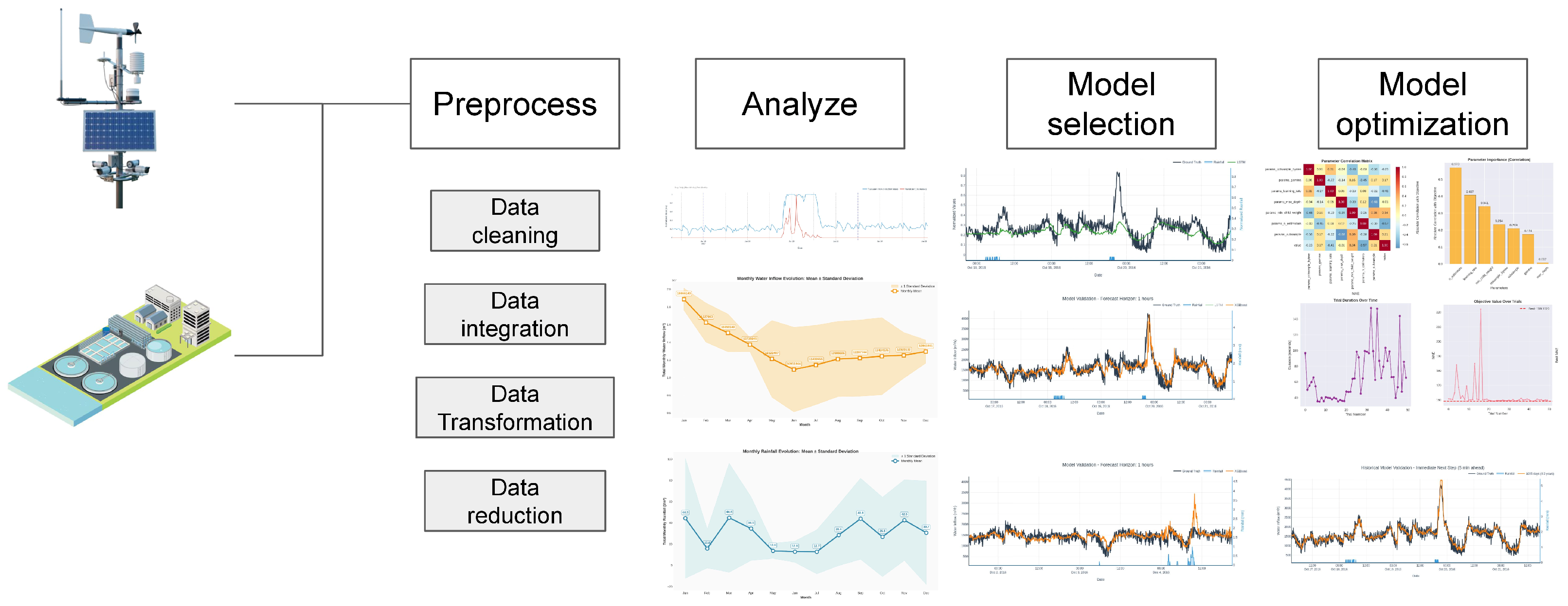
In this study, a data-driven approach was adopted to predict inflow rates in WWTPs, leveraging extensive historical data rather than physical modeling due to the complexity of the underlying processes. For this purpose, Figure 1 depicts the methodology where the first step is to preprocess the different from different sources, the next step consists of analyzing the data and extracting conclusions and insights from the patterns, after that is to test out the selected models and choose the most accurate one, and finally optimize the hyperparameters of the best model.

2.1. Data Acquisition

The dataset was sourced from a WWTP and its own weather station situated along the Spanish Mediterranean coast, comprising a ten-year historical record from 1 January 2012 to 31 December 2022. Two primary variables were selected for their predictive relevance and data completeness: influent flow rate to the WWTP (tagged as the I nfluent_flow_dataset and rainfall (tagged as Rainfall_dataset). Influent flow data were extracted from the flowmeter installed at the entry and saved by the Supervisory Control and Data Acquisition (SCADA) system integrated within the WWTP, while rainfall data were collected from the on-site weather station. These variables were prioritized to maximize temporal coverage and minimize interruptions, as other potential variables, such as chemical oxygen demand or total suspended solids, exhibited frequent malfunctions or incomplete records.

Influent_flow_dataset was quantified in cubic meters per hour (m³/h), representing the volume of wastewater entering the facility. Rainfall_dataset intensity was measured in liters per square meter (l/m²), equivalent to millimeters of precipitation, capturing local weather conditions. Data were recorded at variable intervals ranging from 1 min for the Influent_flow_dataset to 5 min for Rainfall_dataset, providing high-resolution temporal information critical for capturing rapid influent fluctuations associated with Mediterranean climate patterns. It should be noted that during the manuscript, the word timestep will be used to depict each or a set of observations of the time series dataset.

2.2. Data Preprocessing

To ensure data quality and analytical compatibility, the raw time series underwent rigorous preprocessing to address inconsistencies in sampling frequency and data gaps:

• Temporal Synchronization: The SCADA and weather station systems recorded data at different intervals (1 to 5 min). To standardize the temporal resolution, both Influent_flow_dataset and Rainfall_dataset datasets were resampled to a uniform 5-min timestep which is an enough temporal resolution to capture the changing patterns in the desired variables. This process involved computing the mean of measurements within each 5 min window, ensuring temporal alignment across variables without significant loss of information.
• Missing Data Treatment: The datasets were systematically inspected for missing entries. Instances of absent data in either the influent flow or rainfall series, constituting less than 0.5% of the total records, were excluded.
• Outlier Detection: Potential outliers, such as erroneous sensor readings, were identified using a statistical method based on the interquartile range (IQR) [40]. Data points exceeding 1.5 times the IQR beyond the first or third quartiles were flagged and reviewed (compared with maintenance intervals or malfunctioning behavior), with confirmed anomalies removed to prevent model bias. The total number of outliers is less than 0.3%.

Eventually, the synchronized dataset comprised 877,416 observations at 5 min intervals, equivalent to approximately 86,300 hourly records over the ten-year period. The final dataset is tagged as Inflow_Rainfall_dataset during the manuscript.

2.3. Exploratory Graphical Analysis

To elucidate the relationship between rainfall and influent flow, an exploratory data visualization was conducted. This phase aimed to identify temporal patterns, correlations, and event-specific behaviors, particularly during flood-prone periods characteristic of Mediterranean climates.

The dataset was segmented into rainy and non-rainy periods, with rainy days defined as those with measurable precipitation (>0.1 l/m²). Time series evolutions during time were generated using hourly aggregated data to reduce noise from the 5-min resolution.

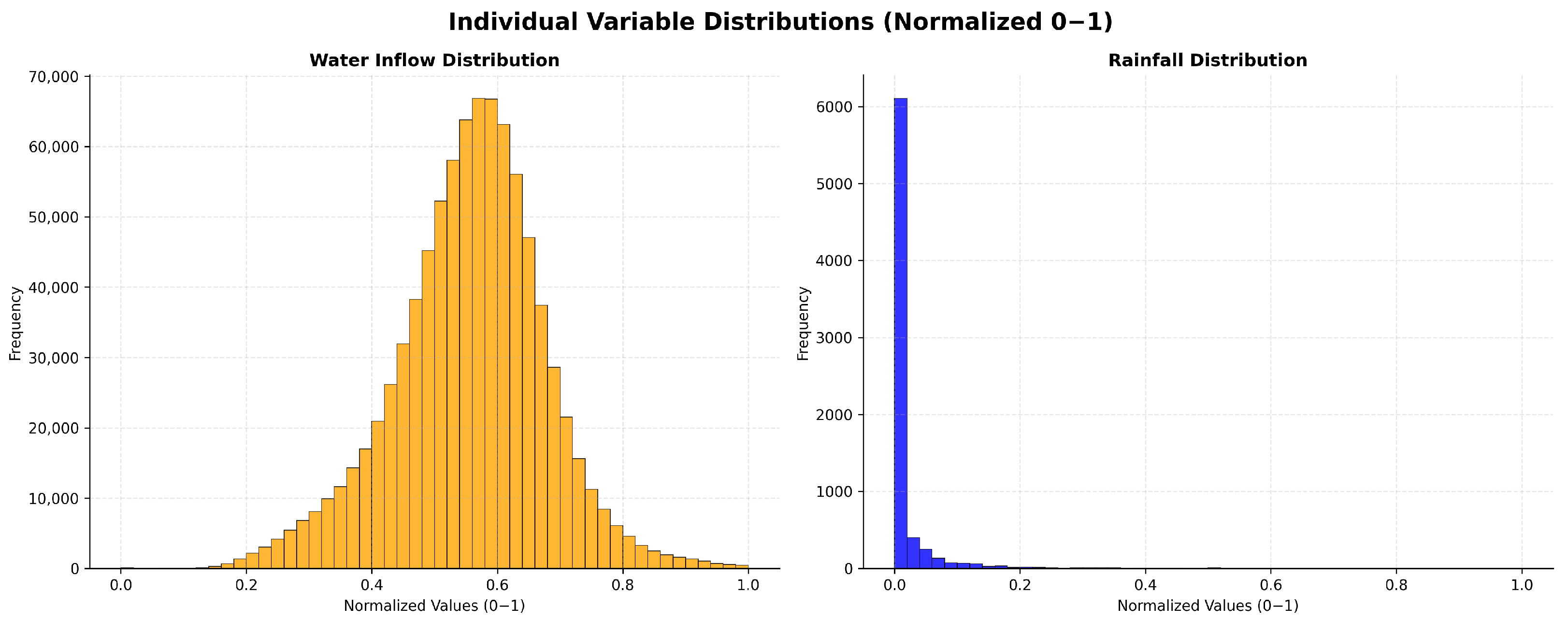
Figure 2 presents the distributions of influent flow and rainfall from Inflow_Rainfall_dataset normalized. The influent flow histogram is approximately unimodal with a central tendency consistent with normal-like dispersion around the mean. By contrast, the rainfall distribution is extremely zero-inflated, which means that the vast majority of bins report no measurable precipitation, and only a small fraction of observations contain non-zero rainfall magnitudes. Quantitatively, rainy timesteps represent approximately 0.83% of the dataset (7306 of 877,416 timesteps), as seen in

Table 1. Summary of same-timestep correlation metrics between rainfall and influent flow (2012–2022).

Metric	All Data	Rain Periods
Sample Size	877,416	7306
Percentage of Timesteps	100%	0.83%
Pearson Correlation	0.1146	0.1009
Spearman Correlation	0.0691	0.1476
Kendall Correlation	0.0564	0.1143
Covariance	3.2166	73.1572
R-squared	0.0131	0.0102
Linear Regression Slope	719.8051	197.1772
Linear Regression Intercept	1556.7829	2244.7253

, indicating a highly imbalanced dataset with sparse event information concentrated in a small temporal subset.

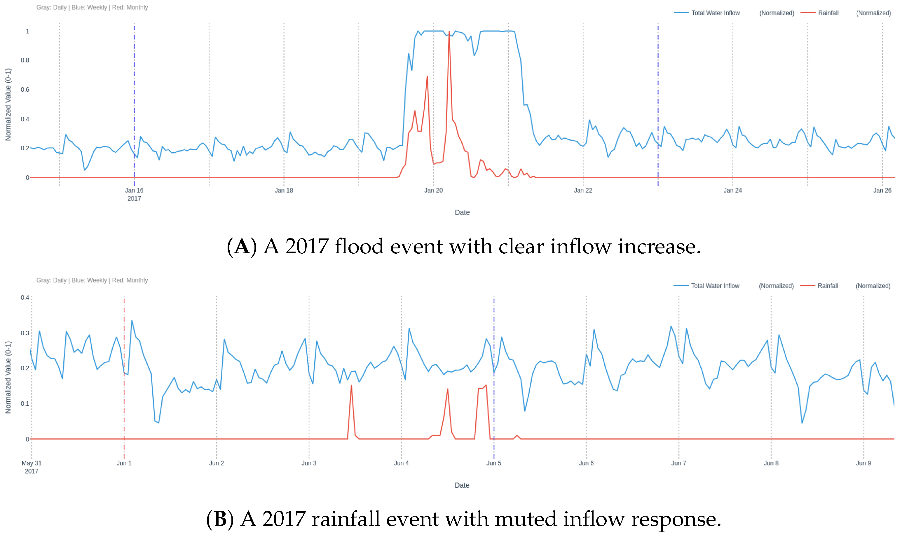
Figure 3 illustrates influent flow responses during rainy periods. Panel (A) depicts a significant rainfall event in 2017, where a clear increase in influent flow coincides with the onset of precipitation, reflecting a rapid catchment response typical of Mediterranean storms. Conversely, panel (B) shows rainfall events in 2017, where the influent flow response is less pronounced, suggesting variability in hydraulic dynamics due to factors such as sewer network buffering or operational interventions.

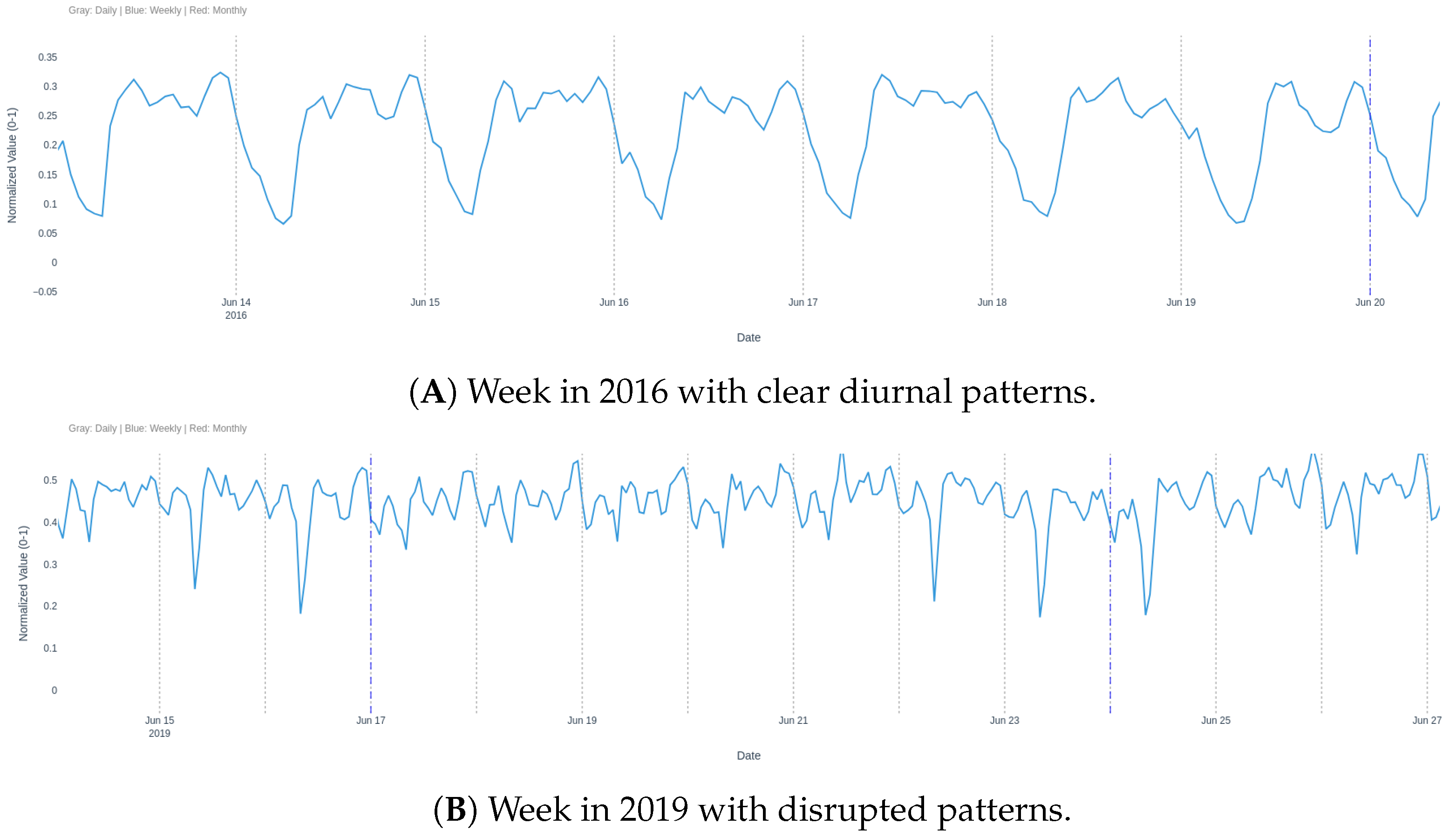
Figure 4 presents influent flow patterns during non-rainy periods. Panel (A) illustrates a week in 2016, showcasing consistent diurnal patterns in influent flow, likely driven by domestic and industrial wastewater contributions. In contrast, panel (B) from 2019 reveals instances where these patterns are disrupted, potentially due to seasonal variations or operational adjustments such as bypass activation.

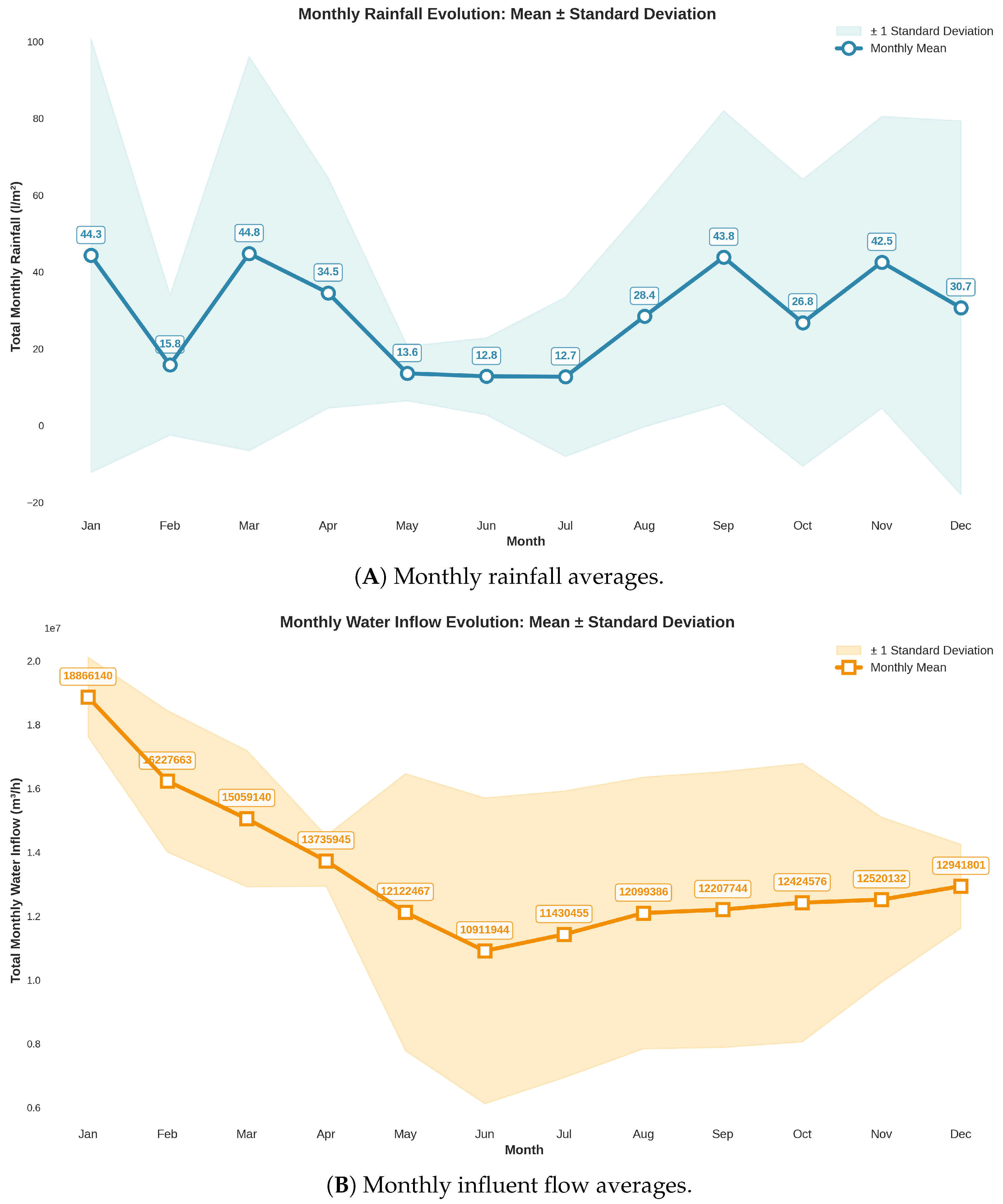
Figure 5 examines the seasonality of rainfall and influent flow during the Inflow_Rainfall_dataset (10 years long). This has been done by adding each observation for each month and calculating the mean for each month. Panel (A) depicts monthly rainfall averages over the ten-year period, revealing low precipitation from May to July, with significant spikes in March, September, and December, which are closely associated with flood seasons in the Mediterranean region. In contrast, panel (B) shows monthly influent flow averages, indicating a lack of clear seasonality, likely due to the influence of non-meteorological factors such as industrial discharges or operational bypasses.

These visualizations reveal that influent flow dynamics vary significantly with the season. For instance operational factors, such as bypass activation during high loads could be the reason.

2.4. Statistical Analysis

A statistical evaluation was conducted to quantify the relationship between rainfall and influent flow. The aim was to characterize the strength, direction, and nature of dependency between the two variables using multiple complementary metrics:

• Pearson correlation coefficient: This metric assesses the strength and direction of a linear relationship between rainfall and influent flow. It assumes normality and linearity, and is particularly informative for detecting proportional co-movements. A high absolute value indicates strong linear dependence.
• Spearman rank correlation coefficient: Spearman’s rho captures monotonic relationships, whether linear or non-linear, by ranking the data before computing correlation. It is robust to outliers and useful when the variables increase or decrease together, but not necessarily at a constant rate.
• Kendall’s tau: Kendall’s tau also measures the strength of monotonic associations but is based on the concordance and discordance of data pairs. It is more conservative than Spearman’s rho and is less affected by sample size, providing a reliable nonparametric measure of ordinal association.

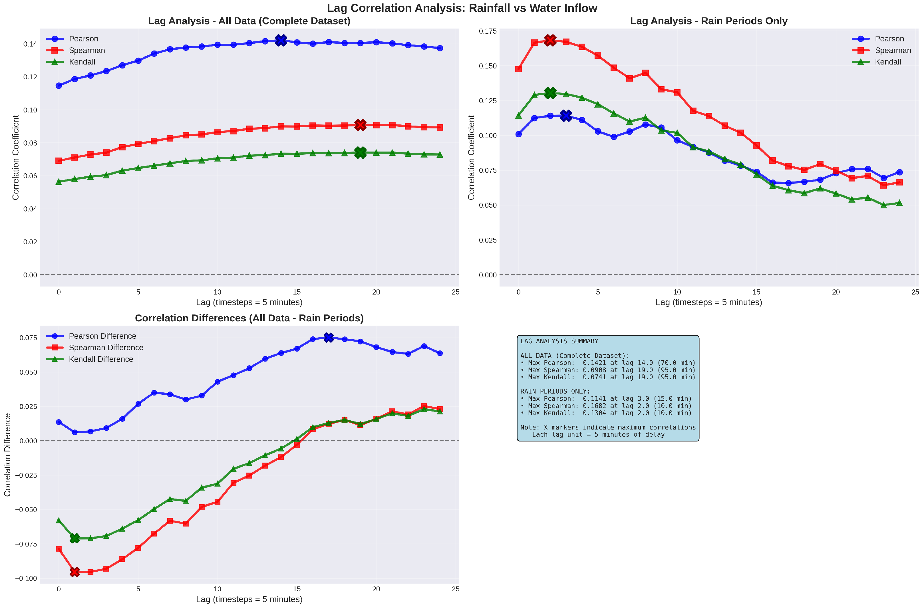
Additionally, a lag analysis was performed to identify the optimal temporal offset between rainfall and influent flow, with lags ranging from 0 to 48 h. Mutual information, covariance, R-squared, and linear regression parameters were also computed to provide a comprehensive understanding of variable interactions.

Table 1 summarizes the correlation metrics for the same-timestep data. For all data (877,416 timesteps), a weak positive Pearson correlation (0.1146) indicates a modest linear relationship, with similar trends in Spearman (0.0691) and Kendall (0.0564) correlations. During rainy periods (7306 timesteps), correlations are slightly stronger, with a Spearman correlation of 0.1476, reflecting non-linear dependencies. Non-rainy periods (870,110 timesteps) show no correlation due to zero rainfall variance, as expected. With this statistical analysis, it can be concluded that there is no linear correlation within the same timestep between influent flow and rainfall.

Figure 6 illustrates the lag analysis, which has the purpose to study whether past data could have linear correlation from the current step, showing the variation in Pearson, Spearman, and Kendall correlations across lags. For all data, the maximum Pearson correlation (0.1421) occurs at a 14-timestep lag, and the maximum Spearman and Kendall correlation (0.0908) at a 19-timestep lag; the fact that both coefficient gets the maximum correlation at the same lag is likely due to their monotonic nature. For rainy periods, correlations peak at shorter lags (Pearson: 0.1141 at the third timestep; Spearman: 0.1682 and Kendall: 0.1304 at the second timestep), indicating a faster influent response during precipitation events. To sum up, even with this lag analysis, influent flow and rainfall lack linear correlations.

2.5. Dataset Construction

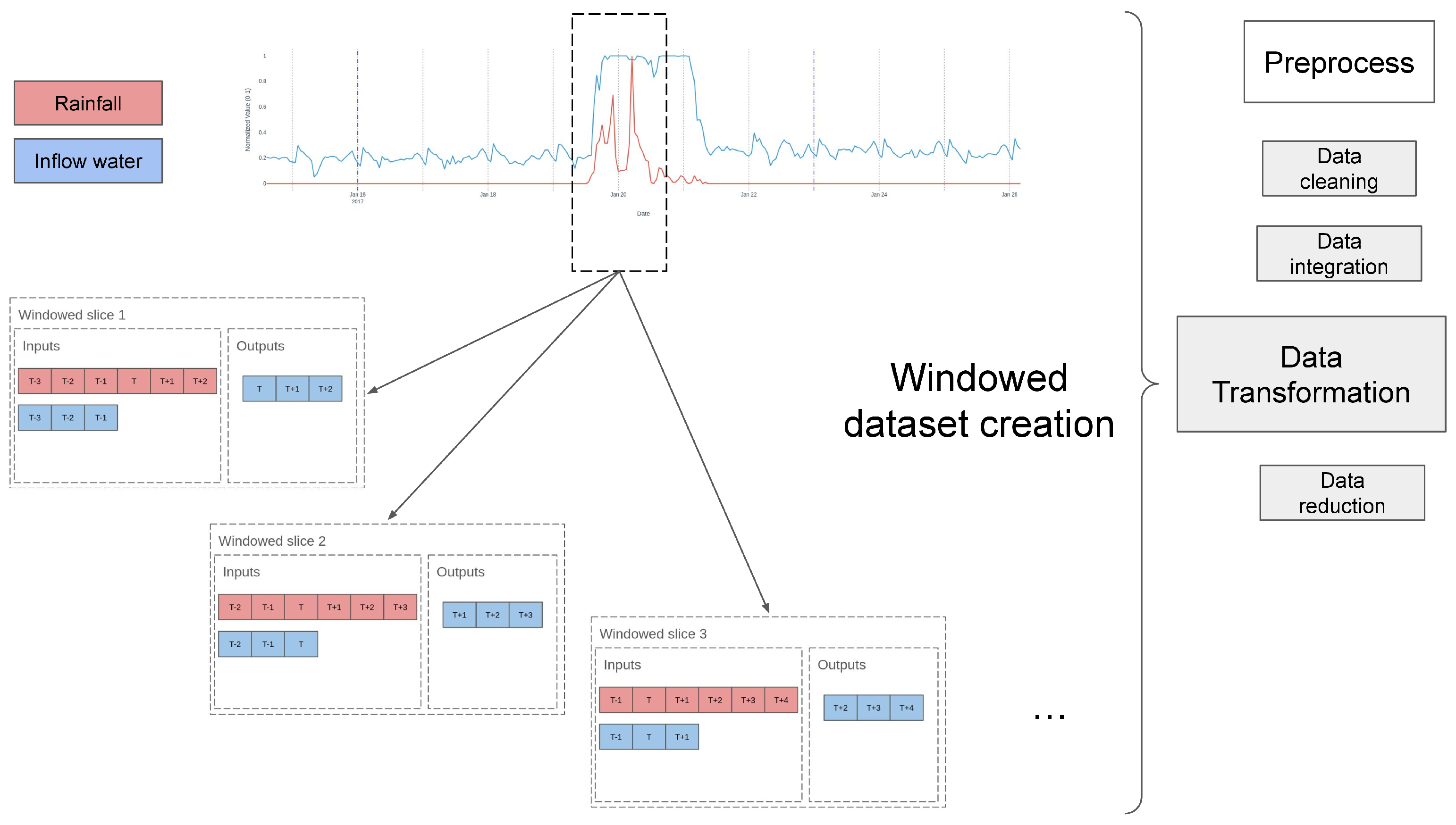
To address the time-series nature of the influent flow prediction problem, a dataset was constructed using a sliding window approach to define input and output sequences from the Inflow_Rainfall_dataset. The prediction output window was fixed at three days (72 h), enabling operational planning for anticipated inflow surges, particularly during flood events prevalent in Mediterranean climates. The input window size, representing historical data, was treated as a hyperparameter, optimized within a search space ranging from 1 to 7 days, with a two-day window selected initially for the model comparison to capture sufficient temporal patterns, including diurnal and weekly cycles, while leveraging three-day forecasts. The new timeseries dataset is tagged as Inflow_Rainfall_ts_dataset.

As previously introduced, the predictive framework was designed to forecast influent flow based on both hydraulic and meteorological information. Specifically, the model inputs comprise sequences of past influent flow and rainfall observations, representing the short-term hydraulic memory of the system, together with forecasted rainfall data, which introduce information about expected upstream conditions. The model expected output corresponds to the forecasted influent flow values over the defined prediction horizon.

The window slicer operated as follows: for each prediction instance, a sequence of historical data (influent flow and rainfall) spanning the input window (576 + 576 timesteps at 5-min intervals which are two days) together with the prediction of the expected rainfall (864 timesteps) of the following three days was paired with a corresponding output sequence of influent flow values for the three-day prediction window (864 timesteps). The slicer incrementally shifted the window across the dataset to generate multiple shifts between input and output sequences, ensuring no overlap. For boosting algorithms like XGBoost, the time-window shifted data is processed by flattening the sequential inputs and outputs into a static feature vector, enabling the model to capture non-linear temporal relationships through iterative tree building and gradient descent, without explicit recurrence as in LSTM.

Figure 7 illustrates the Inflow_Rainfall_ts_dataset construction process, depicting the input window of historical data and the output prediction window, aligned with meteorological forecasts.

2.6. Model Development and Testing

Preliminary statistical and data visualization indicated a weak linear correlation between rainfall and influent flow, suggesting that simple linear models are insufficient for accurately capturing the underlying dynamics. This is largely due to the complex, non-linear, and stochastic behavior of influent flow, particularly during rainfall events.

To address this challenge, a diverse set of predictive models was developed and evaluated using the historical influent flow and rainfall data. The selection encompasses a range of methodological complexity: from baseline models such as the Linear Regressor, to more sophisticated ensemble approaches like Random Forest and Extreme Gradient Boosting, and ultimately to deep learning architectures such as Long Short-Term Memory (LSTM) networks.

Other powerful time series models, such as ARIMA, SARIMA, and Prophet, have been excluded from the study due to their univariate nature.

The complete set of models evaluated in this study is listed as follows:

• Random Forest Regressor (https://scikit-learn.org/stable/modules/generated/sklearn.ensemble.RandomForestRegressor.html, accessed on 4 November 2025): A robust ensemble method handling non-linear relationships and feature interactions, effective for complex datasets [31]. In this study, it serves as a baseline for comparison, leveraging bagging to mitigate overfitting in our imbalanced Inflow_Rainfall_ts_dataset.
• Extreme Gradient Boosting approaches: An advanced ensemble learning technique known for its performance on imbalanced datasets [41,42]. For instance, widely used models like XGBoost [43] and CatBoost [44], will be tested as they incorporate regularization and efficient tree boosting to capture temporal patterns in rainfall-driven inflows, making them suitable for Mediterranean climate variability.
• LSTM Neural Networks: A deep learning model adept at capturing long-term temporal dependencies in time series data [45]. In the current research, it is applied to model sequential influent dynamics, including lagged rainfall and influent flow effects.

All models have been trained with default hyperparameters while the LSTM Neural Network model was designed with four layers of LSTM, Adam optimizer, learning rate of 1 × 10⁻⁴ and 2000 epochs.

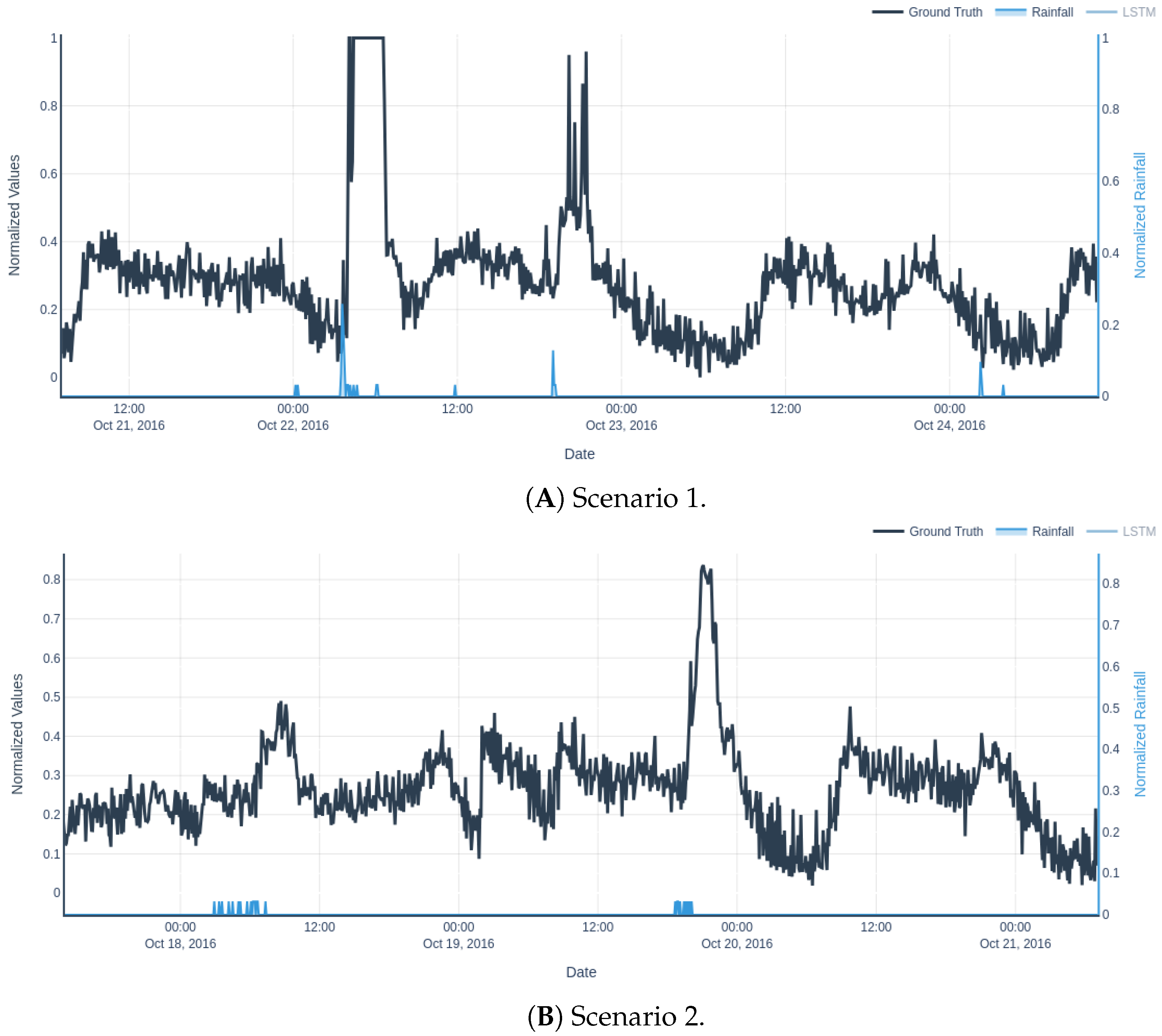
Input features comprised lagged values of rainfall and influent flow to give temporal context to the models, with lag durations (up to 48 h) informed by the lag analysis. The Inflow_Rainfall_ts_dataset was split into training and validation: the first ten years (2012–2022, excluding 2016, which is the most challenging due to being the one presenting more rainy periods) were used for training, and the whole 2016 was reserved for testing, ensuring evaluation on temporally distinct data reflective of operational forecasting scenarios. Moreover, two insightful scenarios are going to be used during the results for comparing the different models and settings where the rain behaves differently in non-linear patterns, making it a proper visual benchmark together with quantitative metrics (Figure 8). During both validation intervals, the foremost part is the spikes placed right after the rainfall moments. It should be noted that all time series plots from now to the end have 5-min observation interval in the X axis.

3. Results and Discussion

This section presents a comprehensive benchmarking of the selected forecasting models with the objective of identifying the most accurate algorithm for predicting influent flow under varying rainfall conditions. The evaluation includes model performance metrics, hyperparameter tuning results, and a sensitivity analysis of the input window size. Additionally, it has been examined whether reliable performance can be achieved using limited training data.

Experiments were executed on the Marenostrum 5 (MN5) supercomputer (https://www.bsc.es/supportkc/docs/MareNostrum5/overview, accessed on 4 November 2025) General Purpose Partition (GPP) for CPU models and Finisterrae 3 Accelerated Partition (ACC) for GPU models. Experiments on MN5 utilized: 2× Intel Xeon Platinum 8480+ 56C 2 GHz, 32× DIMM 64 GB 4800 MHz DDR5, 960 GB NVMe local storage, and ConnectX-7 NDR200 InfiniBand (200 Gb/s bandwidth per node). Experiments on Finisterrae 3 utilized: 256 GB RAM (247 GB usable), 960 GB SSD NVMe local storage, 2× NVIDIA A100 GPUs, and 1 Infiniband HDR 100 connection. Software versions include XGBoost 2.1.4, PyTorch 2.6, and scikit-learn 1.6.1.

3.1. Comparison of Predictive Models

After training and testing the models described in Section 2,

Table 2. Performance comparison of candidate models on the test set. Metrics shown are $R^2$, MSE, RMSE, and total training time.

Model	$\mathbf{MAE}$	$\mathbf{RMSE}$	${\mathit{R}}^2$	Training Time (min)	GPU acc.
Random Forest Regressor	456.45	650.8	0.13	350.3	No
XGBoost	170.1	236.35	0.79	220.8	Yes
CatBoost	183.24	256.28	0.75	205.7	Yes
LSTM	220.3	426.59	0.28	350.1	Yes

summarizes the performance of each model in terms of Mean Absolute Error (MAE), Root Mean Squared Error (RMSE), coefficient of determination ($R^2$) on the test set, training time, and GPU compatibility.

The different metrics are defined as follows:

$$\begin{array}{cc}\hfill \mathrm{MAE}& ={\displaystyle \frac{1}{n}}\sum _{i=1}^n|y_i-{\widehat{y}}_i|,\hfill \end{array}$$

(1)

$$\begin{array}{cc}\hfill \mathrm{RMSE}& =\sqrt{{\displaystyle \frac{1}{n}}\sum _{i=1}^n{(y_i-{\widehat{y}}_i)}^2},\hfill \end{array}$$

(2)

$$\begin{array}{cc}\hfill R^2& =1-{\displaystyle \frac{{\sum }_{i=1}^n{(y_i-{\widehat{y}}_i)}^2}{{\sum }_{i=1}^n{(y_i-\overline{y})}^2}},\hfill \end{array}$$

(3)

where $y_i$ is the observed value, ${\widehat{y}}_i$ is the predicted value, and $\overline{y}$ is the mean observed value. Model performance improves as $R^2$ approaches 1 (indicating better fit), and as MAE and RMSE approach 0 (indicating lower error and greater accuracy). The table also lists total training time.

The results confirm that classical models such as Random Forest with limited expressiveness underperform, particularly under the imbalanced nature of the Inflow_Rainfall_dataset, where only about 1% of observations are associated with rainfall events.

Among the multivariate models, Random Forest showed moderate predictive ability but struggled with temporal dependencies and class imbalance. Surprisingly, LSTM Neural Networks, which are a more advanced architecture, also seem to fail for this type of task. In contrast, ensemble-based Extreme Gradient Boosting methods (XGBoost and CatBoost) exhibited significantly higher predictive accuracy.

Notably, XGBoost emerged as the top-performing model, achieving the highest R² score and lowest error metrics. This is likely due to its ability to model complex non-linear interactions and handle class imbalance through gradient-based optimization and regularized boosting.

For instance the best two models families (Neural Networks and Extreme Gradient Boosting) were chosen with their best models (LSTM and XGBoost) to plot their validation results in the benchmark scenarios with errors depicted in

Table 3. Performance comparison of the two best family models on the validation scenarios. Metrics shown are MAE, RMSE, and R².

Model	$\mathbf{MAE}$	$\mathbf{RMSE}$	${\mathit{R}}^2$	Scenario
XGBoost	219.48	309.82	0.61	1
LSTM	289.1	428.5	0.252	1
XGBoost	280.67	473.97	0.561	2
LSTM	343.1	581.48	0.34	2

where it can be seen that the XGBoost model has higher accuracy in all studied metrics.

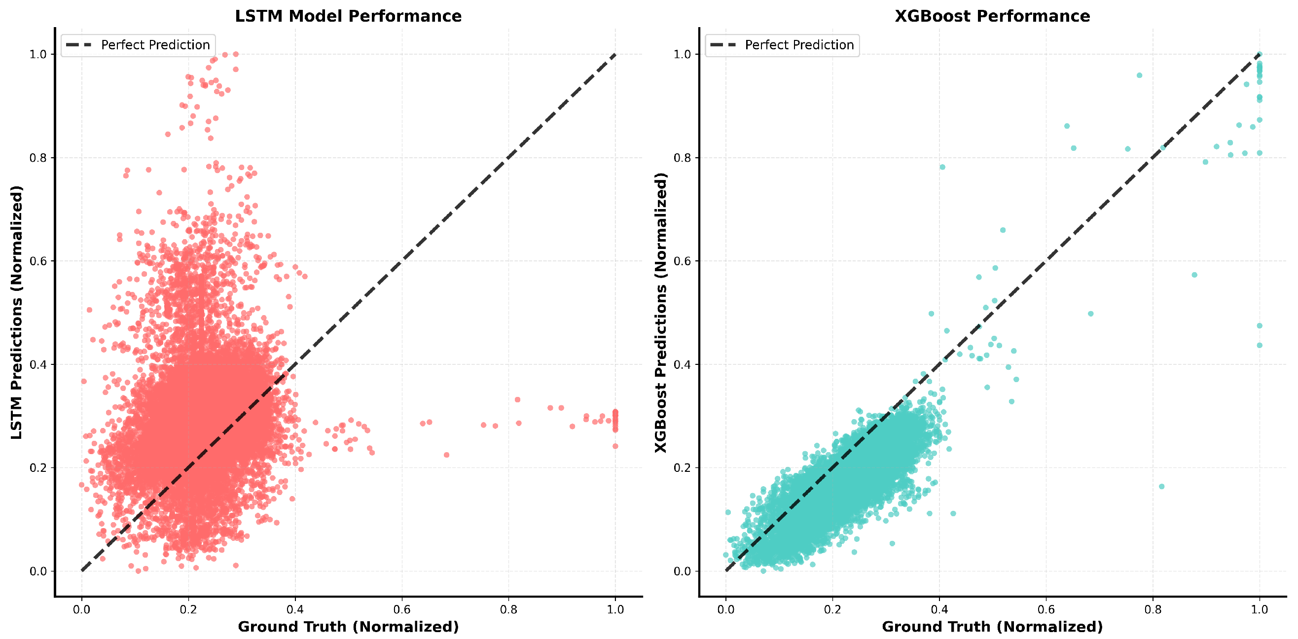
Furthermore, to support the quantitative evaluation with a visual analysis, Figure 9 and Figure 10 depict the predicted influent flow from each model under the two benchmark scenarios. Figure 11 presents scatter plots of predicted versus observed inflow for both models. The XGBoost baseline model predictions tend to align with the 1:1 reference line, with some difficulties in the mid-top values zone. Conversely, the LSTM model displays pronounced underestimation for higher inflow magnitudes—predicted values saturate near 0.4 in normalized units—indicating difficulty in representing extreme events and dynamic scaling.

LSTM exhibits a tendency to over-smooth the output, likely as a consequence of the class imbalance—where only approximately 1% of the training data corresponds to rainfall—thus diminishing its responsiveness to rare but critical rainfall-induced flow spikes. Additionally, its performance deteriorates during non-rain periods, possibly due to overfitting to rare events or the difficulty of learning stable baselines across heterogeneous temporal patterns.

In contrast, XGBoost demonstrates a consistent ability to track both sharp inflow peaks and baseline variations. This robustness across distinct regimes highlights its capacity to model non-linear interactions and respond effectively to rare but impactful events, making it particularly suitable for imbalanced time series problems such as this.

In light of these findings—both quantitative and qualitative —the XGBoost model is selected for subsequent studies. XGBoost’s superior performance stems from its gradient boosting, which adaptively weights rare rainfall events, unlike LSTM’s uniform sequence learning that struggles with <1% imbalance. This highlights ensemble methods’ edge in time series datasets with sporadic extremes.

3.2. Hyperparameter Tuning

To maximize predictive performance, an automated hyperparameter optimization was conducted for the best–performing default model (identified in Table 2 as XGBoost model). Leveraging the Optuna framework [46], which employs Bayesian optimization through the Tree-structured Parzen Estimator (TPE) sampler, we efficiently explored the hyperparameter space by modeling high- vs low-performing regions and prioritizing promising trials. Optuna iteratively suggests and evaluates hyperparameters across a user-defined number of trials (50 in this case), minimizing an objective function (e.g., MSE or RMSE) via adaptive sampling. It is widely used for machine learning models such as LSTM [47] and XGBoost [48,49]. For XGBoost, we focused on hyperparameters influencing tree structure, learning speed, and regularization: max _depth (controls model complexity), learning_rate (step size), n_estimators (number of boosting rounds), subsample and colsample_bytree (sampling ratios for robustness), min_child_weight (minimum leaf node weight for purity), and  gamma (minimum split gain threshold).

The search space together with the best set of hyperparameters found is depicted in

Table 4. Search space for XGBoost together with the best set of hyperparameters.

Hyperparameter	Search Range	Selected	Description
max_depth	$[3,10]$	7	Maximum tree depth
learning_rate	$[0.01,0.1]$	0.078	Step size shrinkage
n_estimators	$[10,200]$	187	Number of boosting rounds
subsample	$[0.5,1.0]$	0.59	Row sampling ratio per tree
colsample_bytree	$[0.5,1.0]$	0.82	Feature sampling ratio per split
min_child_weight	$[1,10]$	3	Minimum sum of instance weight
gamma	$[0,5]$	0.99	Minimum loss reduction threshold

.

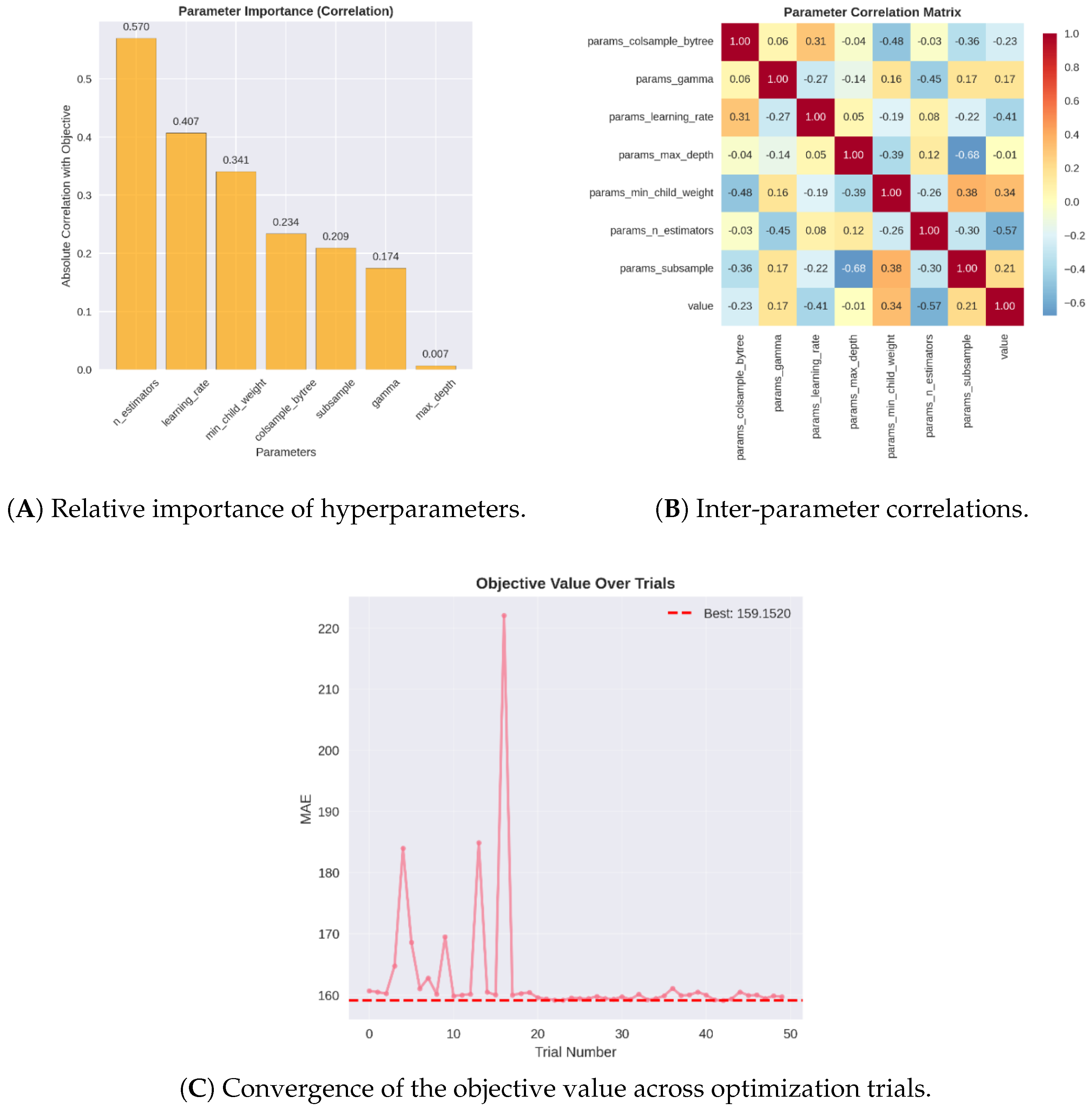
Figure 12 presents visualizations from the hyperparameter optimization process conducted using the Optuna framework. Subplot (A) shows the relative importance of each hyperparameter, indicating that the number of estimators is the most influential parameter (importance score: 0.57), followed by the learning_rate (0.407) and the minimum child weight (0.341). These results indicate that controlling model capacity and the strength of regularization is central to generalization: increasing the number of estimators reduces bias by allowing more additive trees to model complex patterns, whereas a lower learning_rate tempers each tree’s contribution and reduces the risk of fitting noise from rare rain events; min_child_weight acts as a direct regularizer on leaf splits, preventing the model from creating small, highly specific leaves that would disproportionately fit the scarce rainy samples.

Subplot (B) illustrates the pairwise correlation among hyperparameters. A notable positive correlation is observed between the learning_rate and colsample_bytree, as well as between subsample and min_child_weight; in practical terms, the optimizer tended to pair larger step sizes with wider feature sampling (preserving signal per tree), and to pair reduced row sampling with stronger leaf regularization (to avoid spurious splits when fewer examples are used), respectively. Conversely, a negative correlation is detected between subsample and max_depth, which reflects that configurations with deeper trees were typically compensated by more aggressive row subsampling—an implicit regularization strategy that limits overfitting risk when tree complexity increases, a critical consideration given the Inflow_Rainfall_dataset’s class imbalance.

Finally, subplot (C) shows the evolution of the objective function across trials. The optimization converges rapidly, with the best-performing configuration identified around trial 43. Beyond trial 20, incremental improvements become marginal, suggesting the search space is adequately explored by this point.

3.3. Window Size Search

Once the XGBoost model architecture and associated hyperparameters were established, a systematic evaluation was conducted to determine the impact of input sequence length w (measured in 5 min timesteps) on forecasting accuracy and computational efficiency. The window size defines the historical context available to the model from both rainfall and influent flow time series.

In accordance with operational guidelines that mandate a minimum 3-day look-ahead for flood mitigation planning, the analysis considered input windows of $w\in \{288,576,864,1152,1440,1728,2016\}$, corresponding to temporal spans of 1 to 7 days. The forecasting performance—quantified using Mean Absolute Error (MAE), Root Mean Squared Error (RMSE), and coefficient of determination ($R^2$)—as well as the computational cost (training time in minutes), is summarized in

Table 5. Forecasting performance and computational cost as a function of input window length.

Input Window Size	$\mathbf{MAE}$	$\mathbf{RMSE}$	${\mathit{R}}^2$	Training Time (min)
288 (1 day)	167.66	229.91	0.81	95.04
576 (2 days)	169.71	234.87	0.80	157.04
864 (3 days)	170.1	236.35	0.79	220.8
1152 (4 days)	169.31	234.65	0.79	276.96
1440 (5 days)	168.69	232.83	0.8	341
1728 (6 days)	169.79	234.89	0.79	411.52
2016 (7 days)	170.35	235.38	0.79	450.96

.

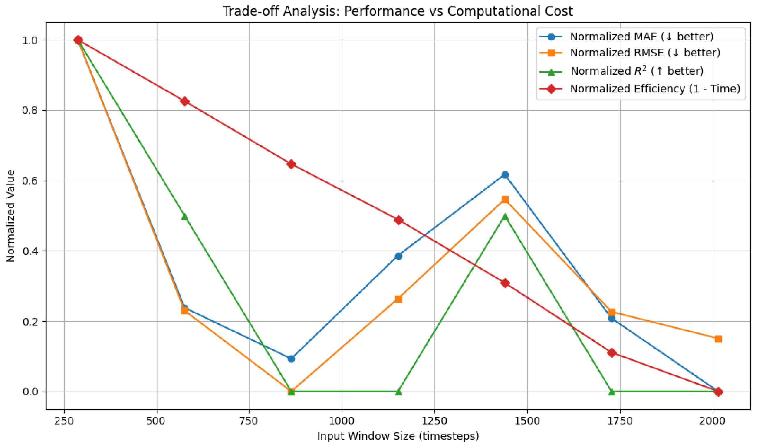
Figure 13 presents a comparative analysis of forecasting accuracy and computational cost across varying input window lengths. The metrics—MAE, RMSE, and coefficient of determination (R²)—are normalized for comparability, as is the inverse of training time to reflect computational efficiency.

The results demonstrate that while increasing the input window beyond 288 timesteps (1 day) leads to marginal improvements in accuracy, these gains plateau quickly. For instance, both MAE and RMSE show negligible reductions beyond the 1-day window, and R² remains relatively stable across longer horizons. In contrast, training time increases with each additional day of historical input, resulting in a steep decline in computational efficiency. This finding suggests that the most informative and influential patterns for influent forecasting are often encoded in short-term temporal dynamics, such as diurnal cycles or rapid rainfall-flow responses. Consequently, a window size of $w=288$ is selected as the optimal configuration.

3.4. Data Availability

With the model architecture, input window length, and hyperparameters already optimized, the next step is to assess how the amount of training data influences forecasting accuracy and computational efficiency. Although the model was initially trained on a large dataset spanning over 9 years, such extensive historical data may not be available in other WWTP use cases, may be impractical to collect for other physical systems, or the storage needed could be prohibitive. Therefore, evaluating the model’s performance with reduced training durations is essential for understanding its applicability to scenarios with limited data availability.

To this end, a dataset size sensitivity analysis was conducted by training the model on varying lengths of historical data, ranging from 14 days to 9 years, while keeping the validation dataset fixed at 2016 (remember this year contains more rainy periods).

Table 6. Forecasting performance and computational cost as a function of training dataset size.

Training Dataset Size	$\mathbf{MAE}$	$\mathbf{RMSE}$	${\mathit{R}}^2$	Training Time (min)
14 days	179.45	247.47	0.79	20.72
21 days	176.069	242.27	0.805	23.36
1 month	171.24	233.6	0.819	25.36
3 month	171.49	235.33	0.816	33.28
6 month	170.38	235	0.817	40.8
1 year	169.75	233.42	0.819	49.6
2 years	168.84	232.48	0.821	70.64
3 years	167.76	229.92	0.825	94.48
9 years	167.2	228.61	0.83	280.56

summarizes the performance metrics for each training set size in terms of MAE, RMSE, R², and training time. It should be note that the training periods have been selected to ensure at least 1% of rainy observations.

The results indicate that most of the performance gain occurs early: increasing the training duration from 14 days to 1 year reduces MAE by 9.7 (5.4%; 179.45 → 169.75), decreases RMSE by 14.05 (5.7%; 247.47 → 233.42), and raises R² by 0.029 (0.79 → 0.819). Additional increases in training size produce rapidly diminishing returns—1 → 2 years yields only a 0.54% MAE reduction (169.75 → 168.84) and a 0.4% RMSE reduction, while 2 → 3 years yields a further 0.64% MAE reduction (168.84 → 167.76) and 1.1% RMSE improvement. Beyond three years, the gains are negligible: expanding from 3 to 9 years reduces MAE by only 0.56 (0.33%) and RMSE by 1.31 (0.57%), while training time increases dramatically (94.48 → 280.56 min, a 2.97× increase). Thus, this suggests that 3 years constitutes a sweet spot for balancing accuracy and computational cost.

A more detailed qualitative assessment is provided in

Table 7. Qualitative analysis of the training dataset amount of data for 14 days, 1 year, 2 years, and 3 years for validation scenario 1 and 2.

Training Dataset Size	$\mathbf{MAE}$	$\mathbf{RMSE}$	${\mathit{R}}^2$	Scenario
14 days	170.1	215.58	0.813	1
1 year	165.61	212.96	0.835	1
2 years	160.26	205.45	0.854	1
3 years	162.15	206.47	0.833	1
14 days	211.55	309.94	0.805	2
1 year	196.1	276.97	0.85	2
2 years	199.12	281.4	0.836	2
3 years	199.95	301.795	0.865	2

, which reports the model’s performance for the two benchmark inflow scenarios under training dataset lengths of 14 days, 1 year, 2 years, and 3 years. In both scenarios, a substantial improvement is observed between 14 days and 1 year. Between 2 and 3 years, the differences are less pronounced and, in some cases, slightly inconsistent—e.g., a marginal degradation in scenario 1 for the 3-year model, possibly due to overfitting or increased noise from long-term data.

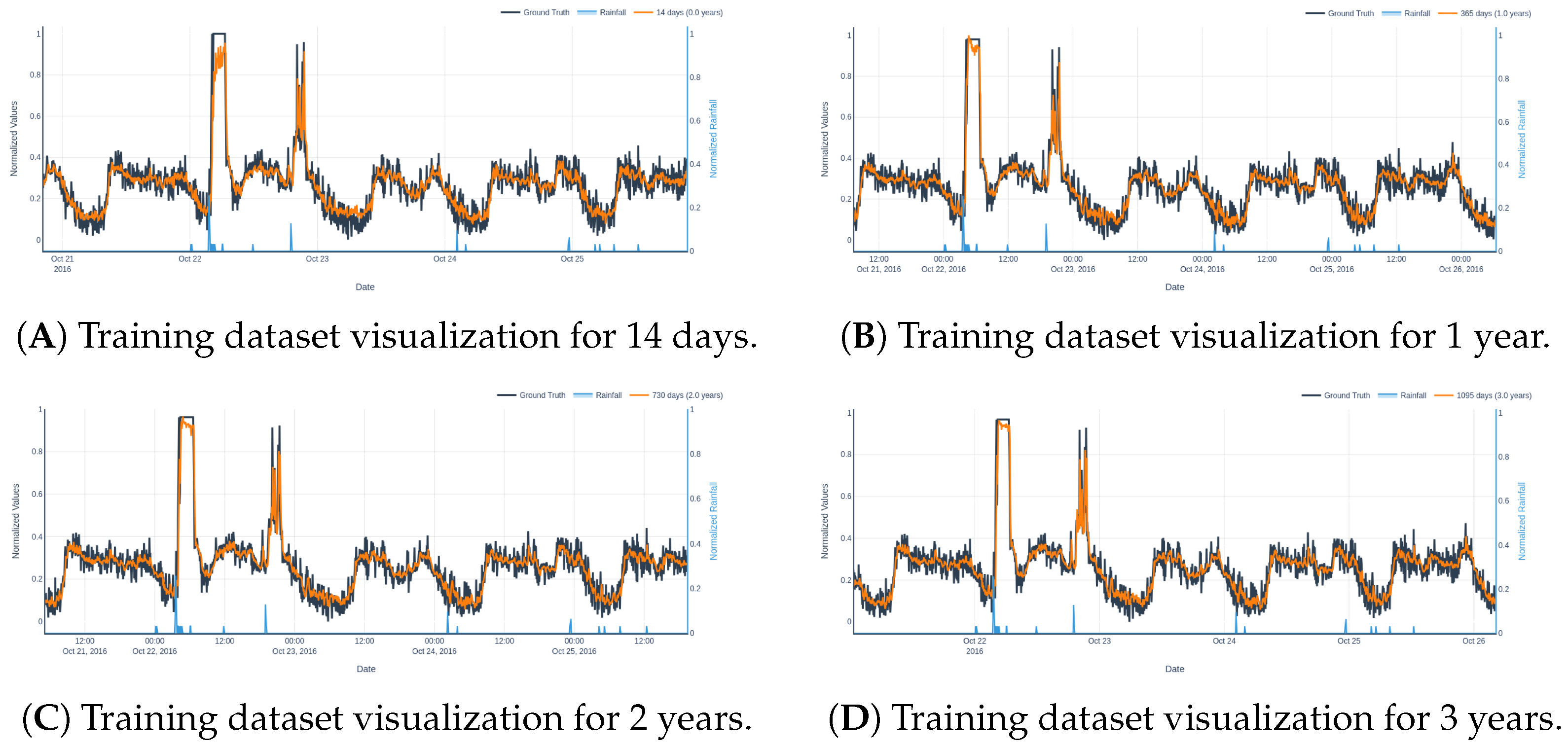
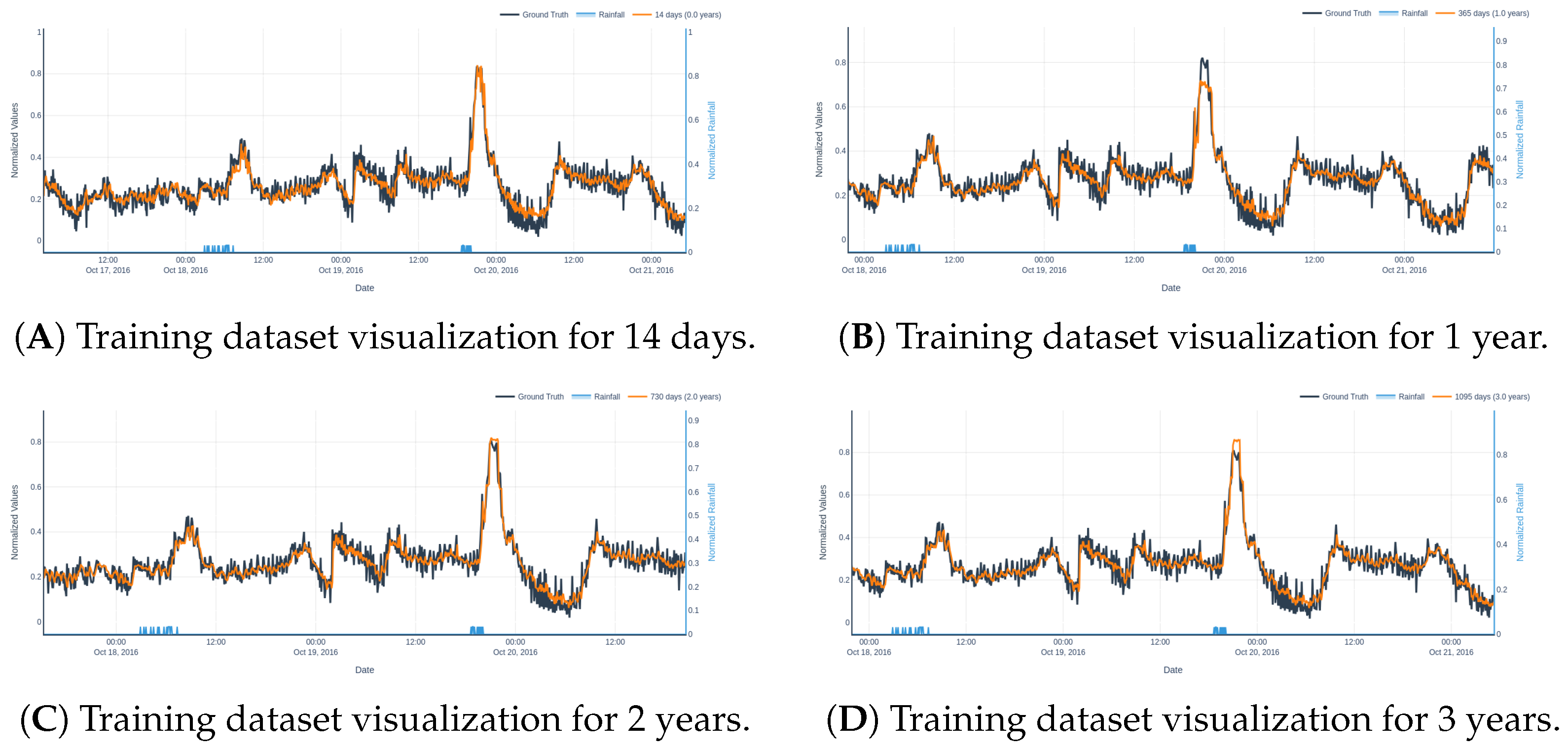
Figure 14 and Figure 15 visualize the predictions across different training durations. In scenario 1, the 2- and 3-year models produce nearly identical predictions, with the 2-year model slightly outperforming in terms of stability. In scenario 2, the 3-year model slightly overshoots the peak inflow, while the 2-year model remains more conservative and accurate.

Importantly, these results highlight the effectiveness of short-duration training: even with only 14 days of training data, the model is capable of capturing key short-term rainfall-inflow dynamics. This robustness makes the proposed XGBoost-based framework highly adaptable to operational contexts with limited historical data, while scaling effectively when larger datasets are available. Furthermore, in an online system where the model continuously infers influent flow as new data is being stored, periodic retraining with the most recent data should be done to maintain accuracy. Such retraining imposes minimal computational demands, as the model’s sweet spot seems to be at a 3-year training size, which only requires approximately 90 min to complete.

3.5. Sliding-Window Validation

To evaluate temporal robustness and sensitivity, the model was trained on fixed three-year windows that were advanced in six-month increments across the available record. For each training window, the immediately following three-month period was used for validation. Evaluation metrics together with the percentage of validation timesteps containing rainfall (Rain%) are included in the summary.

Table 8. Results of the sliding 3-year training window experiment temporarily ordered. Each row reports the training and validation intervals, performance metrics, and rain percentage.

Window	Train Start	Train End	Val Start	Val End	MAE	RMSE	${\mathit{R}}^2$	Rain%
0	11 May 2013	10 May 2016	10 May 2016	8 August 2016	146.243	193.107	0.784	1.5
1	7 November 2013	6 November 2016	6 November 2016	4 February 2017	165.797	226.841	0.887	3.5
2	6 May 2014	5 May 2017	5 May 2017	3 August 2017	106.889	147.989	0.688	0.2
3	2 November 2014	1 November 2017	1 November 2017	30 January 2018	134.400	178.031	0.704	0.3
4	1 May 2015	30 April 2018	30 April 2018	29 July 2018	150.595	200.002	0.833	2.4
5	28 October 2015	27 October 2018	27 October 2018	25 January 2019	137.675	179.062	0.717	1.3
6	25 April 2016	25 April 2019	25 April 2019	24 July 2019	139.407	178.324	0.516	1.0
7	22 October 2016	22 October 2019	22 October 2019	20 January 2020	121.712	162.851	0.694	0.6
8	20 April 2017	19 April 2020	19 April 2020	18 July 2020	83.196	129.497	0.884	0.1
9	17 October 2017	16 October 2020	16 October 2020	14 January 2021	129.813	180.203	0.768	0.6

lists the results for all evaluated windows.

Across the ten windows, the reported metrics display variability. The aggregate statistics are as follows:

• Mean MAE 128.6 (std 23.1); MAE ranges from 83.2 to 165.8.
• Mean RMSE 174.0; RMSE ranges from 129.5 to 226.8.
• Mean R² 0.746; R² ranges from 0.516 to 0.887.
• Rain% in validation windows ranges from 0.1% to 3.5%.

These statistics show variability in model accuracy across the ten randomly selected intervals. However, the performance degradation is strongly associated with periods containing a higher number of rainfall observations: the windows with the largest Rain% (e.g., Window 1 with 3.5% rain) exhibit the highest errors (MAE = 165.8, RMSE = 226.8), followed by windows 0 and 4, also with higher errors and larger Rain% compared to the other windows. Whereas the window with the lowest rain percentage (Window 8, Rain% = 0.1%) attains the best performance (MAE = 83.2, RMSE = 129.5), as also exemplified in windows 2 and 3. These results clearly show that the more rain observations there are in the dataset, the more difficult it is for the model to predict the outcome. However, as seen in Figure 16, the model is still able to properly predict the inflow water in rain periods in both scenarios studied before, clear diurnal patterns, and disrupted patterns.

4. Conclusions and Future Work

4.1. Conclusions

This study successfully preprocessed and analyzed a 10-year historical dataset comprising influent flow and precipitation measurements from a Mediterranean coastal WWTP. Statistical exploration revealed distinct seasonal rainfall patterns and confirmed a highly imbalanced distribution, with rainfall events representing less than 1% of total observations—a key challenge for data driven modeling. A comprehensive comparison of predictive models was conducted, ranging from simple linear regressors to advanced ML techniques. Among these, the Extreme Gradient Boosting (XGBoost) model consistently outperformed alternatives, owing to its ensemble architecture and capacity to handle non-linear, high-dimensional feature interactions. Hyperparameter tuning further refined the model’s predictive performance, identifying the number of estimators as the most influential hyperparameter. Subsequent input window size optimization showed that reducing the input sequence to one day (288 timesteps) significantly decreased training time from 220.8 min to 95.04 min—an approximate 57% reduction—without sacrificing predictive accuracy. Lastly, a dataset size sensitivity analysis demonstrated that the model retains competitive performance even with only 14 days of training data. However, a training dataset spanning approximately three years was found to offer the best trade-off between accuracy and computational cost, suggesting a practical compromise for real-world deployment.

One of the main contributions of this work is operational: it enables translating rainfall forecasts into influent-flow predictions with 3 days of lead time, an interval actionable for decision-making in Mediterranean climates, which are characterized by long dry periods punctuated by intense convective storms. To our knowledge, there was no forecasting tool specifically oriented to WWTP operations in Mediterranean settings that runs in minutes on conventional hardware or in the cloud and provides short-term influent-flow forecasts at the plant level. In practice, this capability supports anticipatory control: operators can ready storm/retention tanks, adjust aeration and pumping setpoints ahead of the first flush, and plan staffing, thereby reducing the likelihood of bypass events and mitigating transient effluent quality degradation during wet weather. Moreover, by scheduling aeration and pumping with a forward-looking view, unnecessary overloads are avoided and energy efficiency is improved.

The approach has clear limitations and safeguards. Forecast skill depends on the accuracy of rainfall predictions, so high-quality, fine-resolution meteorological inputs should be used whenever available, and conservative decisions are advisable under high-risk scenarios. Site-specific factors—such as in-network storage, infiltration/inflow, and local operating strategies. Therefore, thresholds and some input variables must be locally calibrated and periodically reviewed. Data quality is critical: maintaining rain gauges and flowmeters, detecting outliers, and correcting for sensor drift and fouling are essential to prevent biased decisions, especially during extremes.

These findings constitute a promising foundation for the development of operational inflow forecasting tools in WWTPs, offering both scalability and adaptability. In summary, the proposed framework turns already available data streams into a fast, tunable, and uncertainty-aware decision aid for WWTP operation in Mediterranean climates. By enabling preparation hours to days in advance, it supports proactive wet-weather management that protects receiving waters, stabilizes effluent quality, lowers energy and compliance costs, and reduces reliance on bypass. The methodology and insights derived here may serve as a starting point for further research into generalizing data-driven approaches across other components of wastewater treatment systems and beyond.

4.2. Future Work

Future research will focus on extending the predictive framework toward real-time operational integration. Specifically, upcoming developments will embed the model within a digital twin architecture that continuously synchronizes with live sensor data and external meteorological APIs to assimilate rainfall forecasts in real time. This digital twin environment would serve as a virtual replica of the wastewater system, enabling dynamic simulation, scenario testing, and adaptive decision-making under evolving hydrometeorological conditions.

Moreover, future work will explore the interfacing of the predictive engine with Supervisory Control and Data Acquisition (SCADA) systems to enable automated or semi-automated setpoint adjustments based on model forecasts. By linking inflow predictions with SCADA telemetry (e.g., pump status, tank levels, gate positions), operators could anticipate inflow surges and proactively allocate storage, modulate pumping rates, or activate bypass lines before critical thresholds are exceeded. Such integration would transform the framework from a passive forecasting tool into an active decision-support module within a real-time control loop, contributing to operational resilience and energy-efficient management of wastewater infrastructure.

Another critical direction involves quantifying prediction uncertainty. By incorporating confidence intervals or probabilistic forecasting techniques (e.g., quantile regression or Bayesian approaches), the model can better account for the inherent uncertainty in weather forecasts, thereby enhancing its robustness for decision support under uncertainty.

Finally, efforts will be directed toward generalizing the proposed framework to other critical variables in wastewater treatment processes—such as biochemical oxygen demand (BOD), total suspended solids (TSS), and energy consumption—as well as extending the approach to other complex physical systems that exhibit similar spatiotemporal dependencies and non-linear behaviors.