Assessing Climate Change Impacts on Spring Discharge in Data-Sparse Environments Using a Combined Statistical–Analytical Method: An Example from the Aggtelek Karst Area, Hungary

Abstract

This paper introduces a methodology for forecasting spring hydrographs based on projections from regional climate models. The primary study objective was to evaluate how climate change may affect spring discharge. A statistical–analytical modeling approach was developed and applied to the Jósva spring catchment in the Aggtelek Karst region of Hungary. Historical data served to establish a regression relationship between rainfall and peak discharge. This approach is particularly useful for predicting discharge in cases where only historical rainfall data are available for calibration. Baseflow recession was analyzed using a two-component exponential model, with hydrograph decompositionand parameter optimization performed on the master recession curve. Future discharge time series were generated using rainfall data from two selected regional climate model scenarios. Both scenarios suggest a decline in baseflow discharge during different periods of the 21st century. The findings indicate that climate change is likely to intensify hydrological extremes in the coming decades, irrespective of whether moderate or high CO₂ emission scenarios unfold.

1. Introduction

Karst aquifers supply drinking water to about 9.2% of the global population [1], and in countries like Slovenia and Austria, where carbonate rocks are abundant, they provide over half of the total water supply [2]. However, prolonged dry spells can lead to reduced or completely halted spring discharge, threatening the reliability of water supplies that depend on karst systems. Beyond their value as water sources, karst springs also present hazards to human populations. Sudden spring flow surges can cause flash floods, posing risks to infrastructure and public safety. Additionally, the rapid movement of contaminants through karst conduits during such events can lead to bacterial outbreaks, creating serious public health concerns.

According to projections from the Intergovernmental Panel on Climate Change (IPCC) and similar organizations, the remainder of the 21st century will be marked by substantial increases in temperature and significant shifts in precipitation patterns [3,4,5]. These changes in climate conditions are expected to affect extreme weather events, leading to increases in their intensity, frequency, spatial extent, duration, and unusual timing. As a result, there is growing concern about the potential for unprecedented extreme events to occur [6]. Observations since 1950 have already shown changes in some extreme weather conditions resulting from anthropogenic factors like increased greenhouse gas concentrations. Droughts have become more intense and longer lasting in certain regions since the 1950s due to decreased precipitation and/or increased evapotranspiration. These trends are predicted to continue into the 21st century across many areas globally.

Additionally expected is an increase in heavy rainfall events, primarily at high latitudes and tropical regions throughout this century—especially during winter months within northern mid-latitudes—resulting from continued warming caused by greenhouse gas emissions. While total precipitation may decrease in some regions due to climate change effects, heavy rainfall intensity is projected to increase [7]. Climate change variables directly impact hydrological cycles by influencing surface runoff rates, evapotranspiration levels, and recharge rates [8]. For instance, karst aquifers exhibit strong correlation between their spring discharge rates with rainfall amounts. It is therefore clear that climate change directly affects water supplies dependent on karst springs [9].

The primary aim of this paper is to introduce a methodology for predicting spring discharge time series using projections from regional climate models. A further objective is to present an approach that remains effective in data-sparse environments, where rainfall data are the only resource available for model calibration. To address these goals, a combined statistical–analytical modeling framework was developed. The methodology is demonstrated using data from the Jósva spring catchment, situated in Hungary’s Aggtelek Karst area.

2. Precedents

Numerous researchers have sought to mathematically characterize spring hydrographs to predict spring discharge. These methods can be classified based on the time scale of the analyzed hydrographs and the degree to which they represent physical processes within karst systems.

Time series analysis represents one such approach, focusing on sequences of recharge events in karst hydrographs. These methods employ mathematical transformations whose results are not directly tied to physical properties, yet they are effective for analyzing long-term datasets and accounting for uncertainties in rainfall, recharge, and aquifer behavior. Pioneering work in this field was conducted by Jenkins and Watts [10], with subsequent contributions from Mangin [11,12,13,14], who first applied time series analysis to investigate the functioning of karst aquifers. Other notable studies include those by Padilla and Pulido-Bosch [15], Larocque et al. [16], Grasso [17], and Grasso and Jeannin [18,19]. Fiorillo et al. [20] investigated statistical correlations between rainfall and discharge, while Fiorillo and Doglioni [21] applied cross-correlation techniques to analyze this relationship for two karst springs in southern Italy. Reservoir (or bucket) models represent simplified systems that link rainfall input to spring discharge output. These traditional approaches, as described by Mero [22,23], Mero and Gilboa [24], Bezes [25], and Thiéry [26], typically use one reservoir to represent low-permeability matrix flow and another for high-permeability conduit flow. More recent models, such as that proposed by Bailly-Comte et al. [27], employ a parallel reservoir configuration, allowing for the simulation of gradient inversions and flow reversal between conduits and the surrounding rock matrix.

Analytical methods provide insight into the hydraulic properties of karst aquifers. One-dimensional solutions, like those from Boussinesq [28] and Berkoff [29], and two-dimensional solutions from Kovács [30] and Kovács et al. [31] demonstrate that the recession coefficient (α) is proportional to T/SL², where T denotes transmissivity, S represents storativity, and L is the block size. These relationships allow for the estimation of conduit spacing and matrix properties through hydrograph recession analysis.

Artificial neural networks (ANNs) and deep learning (DL) approaches offer data-driven alternatives that do not require prior knowledge of system structure. ANNs are especially useful for capturing nonlinear relationships. The multilayer perceptron in particular can approximate any differentiable function [32,33]. In hydrology, ANNs have proven effective in modeling rainfall–discharge or water level relationships [34,35,36,37]. For karst systems, their utility has been demonstrated in short-term spring discharge forecasting [38,39]. More recent studies aimed to align ANN outputs with physically interpretable components. Kong-A-Siou et al. [40] developed models linking rainfall to both water level and discharge, whereas Dubuis et al. [41] applied a semi-distributed lumped modeling approach using the MIKE SHE platform to investigate the effects of climate change on a karst catchment in Lebanon. Their model divided the catchment into subunits, each represented by interconnected reservoirs.

In summary, a range of methods has been developed to simulate and predict spring discharge, each with specific strengths and limitations. Ongoing research seeks to integrate the spatial–temporal flexibility of statistical approaches with the physical interpretability offered by analytical techniques, aiming to enhance the reliability and explanatory power of karst hydrological models.

3. Materials and Methods

3.1. Hydrograph Features

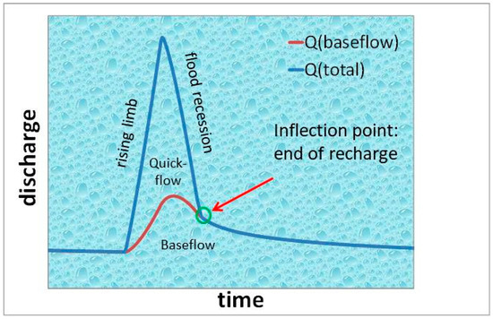
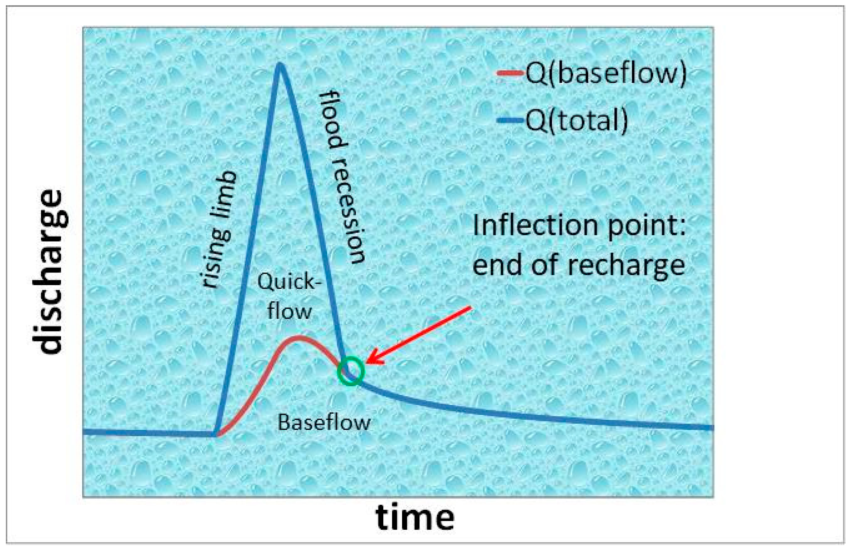
Spring hydrographs illustrate how spring discharge changes over time, typically showing distinct peaks that reflect the aquifer’s response to recharge events. Each peak consists of a rising limb followed by a falling limb. The inflection point on the falling limb marks the end of direct recharge. The steeper portion before this point is termed the flood recession, while the gentler slope afterward is called the baseflow recession (Figure 1). Quickflow arises from direct recharge through sinkholes and vertical shafts, which convey water from sinking streams and the epikarst into the conduit network. Baseflow, in contrast, originates from the slow release of water stored within low-permeability matrix blocks and is less affected by short-term rainfall variability. Matrix recharge occurs via diffuse infiltration from the land surface and through gradient inversion near conduits—a process commonly known as bank storage.

Figure 1. Characteristic features of a hydrograph peak.

3.2. Hydrograph Analysis

Boussinesq [28] and later Maillet [42] were the first to provide mathematical models for baseflow recession (Equation (1)):

$$Q_{\left(t\right)}=Q_0{e}^{-\alpha t}$$

(1)

where Q_t represents discharge (L³T⁻¹) at time t and Q₀ is the initial discharge (L³T⁻¹) at an earlier time. The parameter α is the recession coefficient (T⁻¹), typically expressed in units of days.

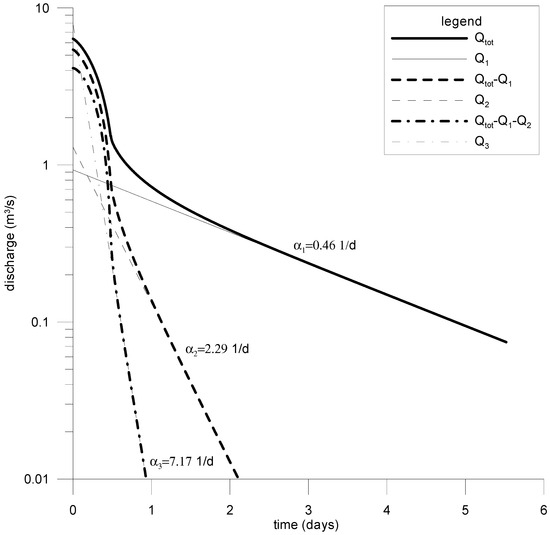
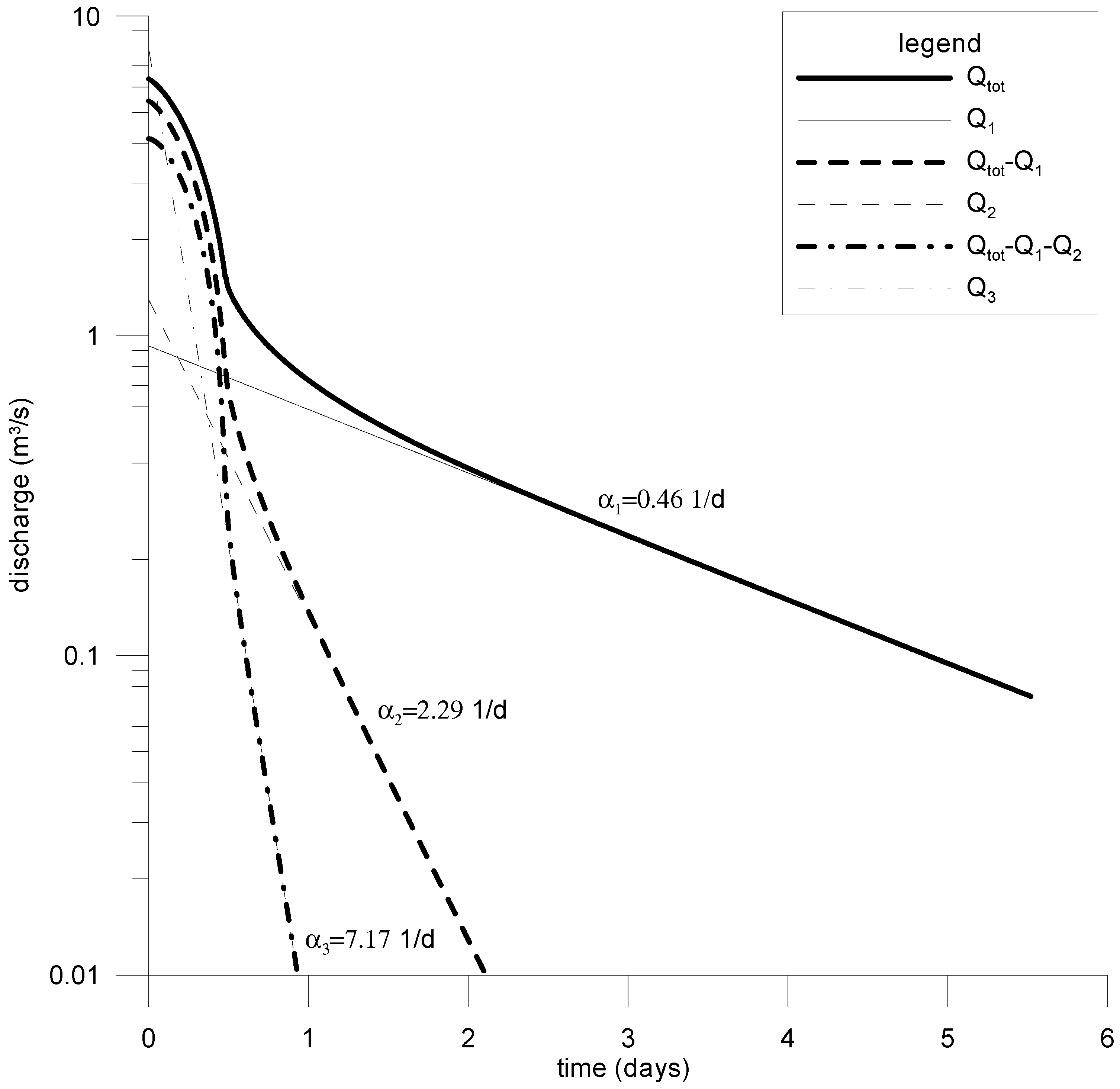
When the exponential recession equation is plotted on a semi-logarithmic scale, it forms a straight line with slope α. This formulation is generally appropriate for describing baseflow conditions in karst systems during low-water stages. However, in the earlier stages of baseflow recession, the discharge often deviates from Maillet’s [42] simple exponential baseflow model. Forkasiewitz and Paloc [43] observed that the falling limb of hydrograph peaks can usually be segmented into multiple exponential components—most often three. This observation led to the development of the hydrograph decomposition approach. In this method, exponential functions are first fitted to the flattest portion of the spring hydrograph, then sequentially subtracted from the residual curve to isolate the individual components of the recession (see Figure 2).

Figure 2. Hydrograph decomposition according to the concept of Forkasiewitz and Paloc [43].

Forkasiewitz and Paloc [43] proposed that the distinct segments of a spring hydrograph peak correspond to the discharge contributions of separate parallel reservoirs, each draining simultaneously into the spring (Equation (2)).

$$Q_{\left(t\right)}=Q_1{e}^{-{\alpha }_{1}t}+Q_2{e}^{-{\alpha }_{2}t}+Q_3{e}^{-{\alpha }_{3}t}$$

(2)

Schoeller [44] suggested that the successive exponential segments observed on the falling limbs of spring hydrographs result from transitions between different flow regimes, such as from turbulent to laminar flow.

Kovács [30] and Kovács et al. [30] derived an exact analytical solution for baseflow recession. Later, Kovács and Perrochet [45] showed that baseflow recession can be expressed as the sum of an infinite series of exponential terms (Equation (3)). Their findings suggest that these exponential components do not necessarily correspond to separate permeability zones, but instead reflect transient processes linked to the gradual release of water from low-permeability matrix blocks.

$$Q_{\left(t\right)}={\displaystyle \sum _{i=1}^n}{Q}_i{e}^{-{\alpha }_{i}t}$$

(3)

3.3. Analytical Solution

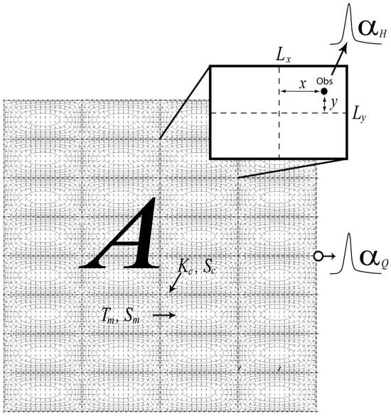
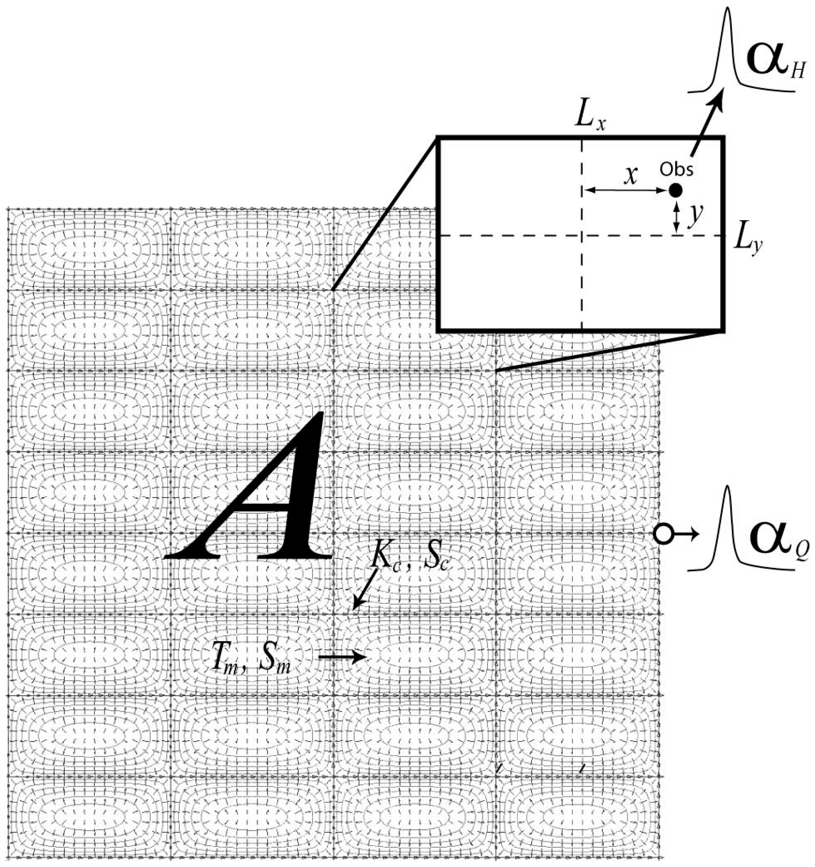
The analytical solutions by Kovács [30] and Kovács et al. [31] and later refined by Kovács and Perrochet [45,46] are based on the conceptual karst model shown in Figure 3. This model consists of a rectangular conduit network embedded within a low-permeability rock matrix, creating discrete matrix blocks, with a single outlet representing the karst spring. Despite its simplicity, the model effectively captures key hydrodynamic behaviors and can be fully described by specifying the hydraulic properties of the matrix and conduits, the spacing between conduits, and the areal extent of the low-permeability matrix blocks within the aquifer (Figure 3).

Figure 3. Conceptual model of karst systems. T_m (L²T⁻¹) denotes matrix transmissivity, S_m (-) is matrix storativity, K_c (L³T⁻¹) represents conduit conductance, S_c (L) is conduit storativity, A (L²) is catchment area, and L_x and L_y (L) are block dimensions. The coordinates x and y represent the distance of the observation well from the block center. α_H and α_Q are well and spring hydrograph recession coefficients. After Kovacs and Perrochet [45].

An analytical solution describing the diffusive flux from a two-dimensional asymmetric rectangular block, bounded by uniform head conditions, is given by the following expression (Kovács and Perrochet [45], Equation (4)):

$$Q_{\left(t\right)}={\displaystyle \frac{64T{H}_0}{{\pi }^2}}\left\{\beta {\displaystyle \sum _{n=0}^{\infty }}{e}^{-a{\beta }^2(2n+1{)}^2}{\displaystyle \sum _{n=0}^{\infty }}{\displaystyle \frac{e^{-a(2n+1{)}^2}}{(2n+1{)}^2}}+{\displaystyle \frac{1}{\beta }}{\displaystyle \sum _{n=0}^{\infty }}{e}^{-a(2n+1{)}^2}{\displaystyle \sum _{n=0}^{\infty }}{\displaystyle \frac{e^{-a{\beta }^2(2n+1{)}^2}}{(2n+1{)}^2}}\right\}$$

(4)

where the initial conditions assume a uniform hydraulic head distribution across the block surface, expressed as follows (Equation (5)):

$$a={\displaystyle \frac{{\pi }^{2}Tt}{S{L}_x^2}}\mathrm{and}\beta ={\displaystyle \frac{L_x}{L_y}}$$

(5)

where T (L²T⁻¹) is block transmissivity, S (-) is block storativity, L_x and L_y (L) are block size, and β (-) is the asymmetry factor. Equation (6) follows from Equation (4):

$$Q_{\left(t\right)}=={\displaystyle \frac{64}{{\pi }^2}}{H}_{0}T\left\{\begin{array}{l}(\beta +{\displaystyle \frac{1}{\beta }})e^{-a\left(1+{\beta }^2\right)}+(\beta +{\displaystyle \frac{1}{9\beta }})e^{-a\left(1+9{\beta }^2\right)}+({\displaystyle \frac{\beta }{9}}+{\displaystyle \frac{1}{\beta }})e^{-a\left(9+{\beta }^2\right)}+({\displaystyle \frac{\beta }{9}}+{\displaystyle \frac{1}{9\beta }})e^{-9a(1+{\beta }^2)}+\\ +({\displaystyle \frac{\beta }{25}}+{\displaystyle \frac{1}{25\beta }})e^{-25a(1+{\beta }^2)}+({\displaystyle \frac{\beta }{9}}+{\displaystyle \frac{1}{25\beta }})e^{-a(9+25{\beta }^2)}+({\displaystyle \frac{\beta }{25}}+{\displaystyle \frac{1}{9\beta }})e^{-a(25+9{\beta }^2)}+\\ +(\beta +{\displaystyle \frac{1}{25\beta }})e^{-a(1+25{\beta }^2)}+({\displaystyle \frac{\beta }{25}}+{\displaystyle \frac{1}{\beta }})e^{-a(25+{\beta }^2)}+\cdots \end{array}\right\}$$

(6)

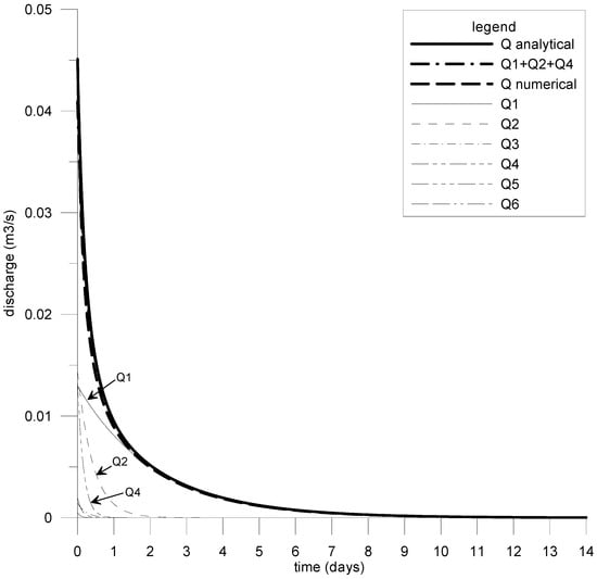
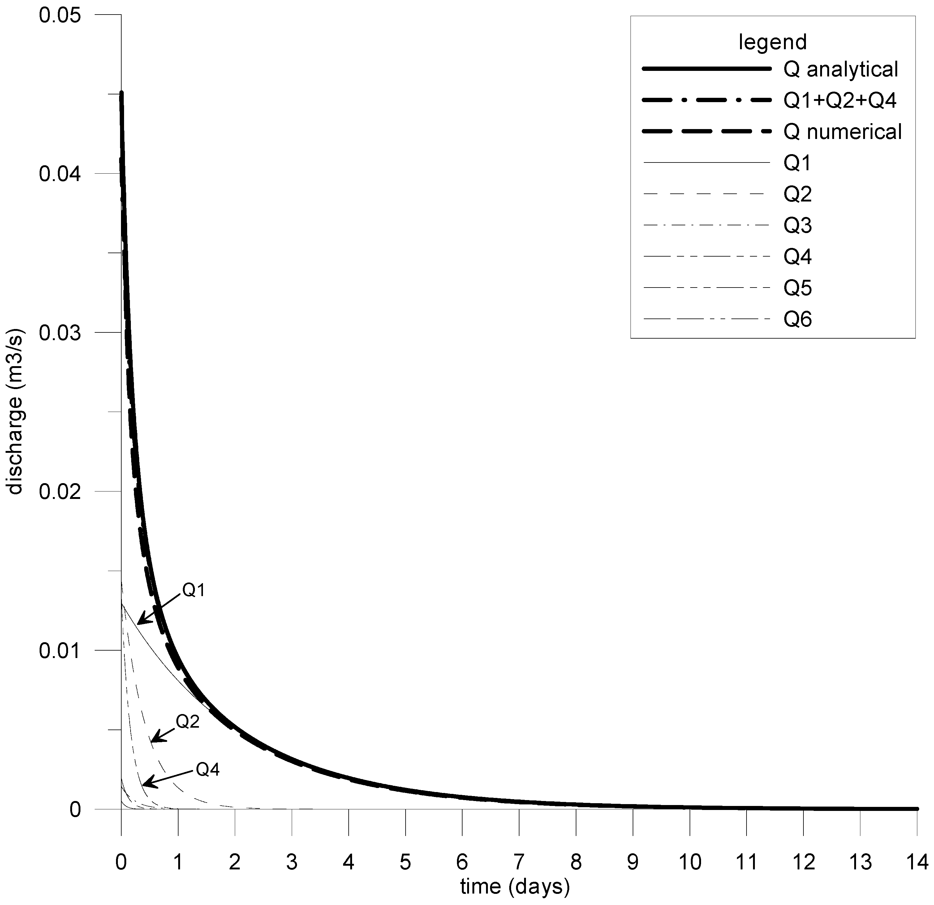
Kovács and Perrochet [45] demonstrated that baseflow can be modeled as the sum of an infinite series of exponential components. However, they observed that higher-order terms quickly become insignificant during the early phases of the recession. Consequently, they concluded that baseflow recession can be effectively approximated using just three exponential components, as illustrated in Figure 4.

Figure 4. Exponential components of the analytical solution of Kovacs and Perrochet [45].

Kovács et al. [47] applied the two-dimensional analytical solution to determine hydraulic and geometric parameters and to investigate the hydrodynamic behavior of the Bükk Karst system in northeastern Hungary. Building on the analytical framework, Kovács [48] developed a quantitative classification method for highly heterogeneous hydrogeological systems, including karst and fractured aquifers. More recently, Kovács and Stevanovič [49] proposed a combined statistical–analytical approach for modeling spring discharge.

3.4. Methodology

Traditionally, reservoir models have been widely used for spring discharge modeling. These models define a direct mathematical relationship linking rainfall to spring discharge. However, this approach requires accurate data on both rainfall and evapotranspiration, the latter being particularly challenging to estimate reliably, especially when no field measurements are available. Additionally, the method assumes that climate variables are uniform across the entire catchment area within each time step, which may not hold true in reality.

There are inherent limitations when applying a one-dimensional model to spatially distributed systems. Due to these uncertainties, relying solely on rainfall data to predict spring discharge can be problematic or even misleading. Although daily rainfall often correlates well with discharge peaks, this relationship is considerably weaker for spring baseflow. This difference stems from the dual hydraulic behavior of karst systems: hydrograph peaks (floods) result from direct recharge, while baseflow arises from the delayed release of water stored in low-permeability matrix blocks after infiltration. Since baseflow responds more slowly than rainfall and flood peaks, it cannot be reliably represented by a single regression function. Thus, while flood discharges can be reliably estimated using regression models relating rainfall to discharge, baseflow necessitates the use of physics-based analytical functions. The proposed method involves developing regression relationships between rainfall and flood discharge, and simulating flood discharge based on future rainfall projections from regional climate models. This approach assumes that evapo-transpiration during heavy rainfall events is negligible due to saturated atmospheric conditions, a hypothesis supported by comparisons with multi-component regression models that include evapotranspiration.

Baseflow components of spring discharge were modeled using two-dimensional analytical solutions developed by Kovács [30], Kovács et al. [31], and Kovács and Perrochet [45], with fitting parameters calibrated from historical rainfall and discharge data.

The prediction of future spring discharge time series involved several key steps:

• Selection of climate projections representing future conditions, including the RCP4.5 and RCP8.5 radiative forcing scenarios (see Table 1).
  Table 1. Regional climate model projections investigated.

  GCM	RCM	Scenario	Scenario Number
  IPSL-IPSL-CM5A-MR	SMHI-RCA4	RCP45	1
  CNRM-CERFACS-CNRM-CM5	SMHI-RCA4	RCP85	2

• Identification of hydrograph peaks and compilation of a peak discharge dataset.
• Development of regression models to quantify relationships between rainfall and peak discharge.
• Construction of master recession curves (MRCs) to determine recession coefficients and separate baseflow components.
• Simulation of spring discharge during the calibration period using observed rainfall, followed by comparison with measured hydrographs.
• Calibration of the combined statistical–analytical model by adjusting initial baseflow parameters.
• Prediction of spring discharge using rainfall time series from regional climate model (RCM) projections for the forecast period.
• Analysis of predictive results using descriptive statistics.

For the climate projections, the EURO-CORDEX ensemble was used, focusing on representative concentration pathway (RCP) scenarios [50,51]. Specifically, RCP4.5 and RCP8.5 were selected, corresponding to additional radiative forcing of 4.5 W/m² and 8.5 W/m², respectively, by 2100 relative to pre-industrial levels. Under RCP8.5, greenhouse gas emissions continue rising throughout the 21st century, leading to a projected global near-surface air temperature increase of 2.6–4.8 °C during 2081–2100 compared to 1986–2005 [52], reflecting current CO₂ emission trends. In contrast, RCP4.5 assumes emissions peak around 2040 and then decline, resulting in a projected temperature rise of 1.1–2.6 °C over the same period relative to 1986–2005 [50]. Although more moderate, RCP4.5 still predicts that near-surface global temperatures are likely to exceed a 2 °C increase by the end of the century compared to 1850–1900 [52]. Table 1 summarizes the selected climate model ensemble projections used in this study. Bias-corrected rainfall data were applied following Szabó et al. [53].

4. Test Site

The Aggtelek Karst, located along the Hungarian–Slovakian border, is part of the Western Carpathian mountain range. It constitutes the southern section of the Gömör–Torna Karst in northeastern Hungary and is closely connected geologically and hydrographically to the Slovak Karst. The region is renowned for its complex and diverse cave systems and karst formations [54]. Tropical–subtropical karstification shaped the area during the Late Cretaceous and Paleogene, while periglacial geomorphological processes dominated during glacial periods. Since 1995, the Aggtelek Karst, together with the Slovak Karst, has been designated a UNESCO World Heritage Site. This karst system is a prime example of a plateau karst shaped under a humid temperate climate. Intense karstification of Triassic limestones has created numerous surface and subsurface karst features, including over 285 caves. The Baradla–Domica cave system, the most extensive in the region, extends for more than 30 km and is classified as a water-table cave. The karst plateaus are also densely dotted with shaft caves, with densities reaching up to 40 shafts per square kilometer on the Alsó-hegy plateau.

The Aggtelek Karst is composed of limestone plateaus running east–west at elevations between 400 and 600 m above sea level. Deep valleys, carved between these plateaus, lie at elevations ranging from 200 to 260 m. The massif primarily consists of Triassic sedimentary rocks.

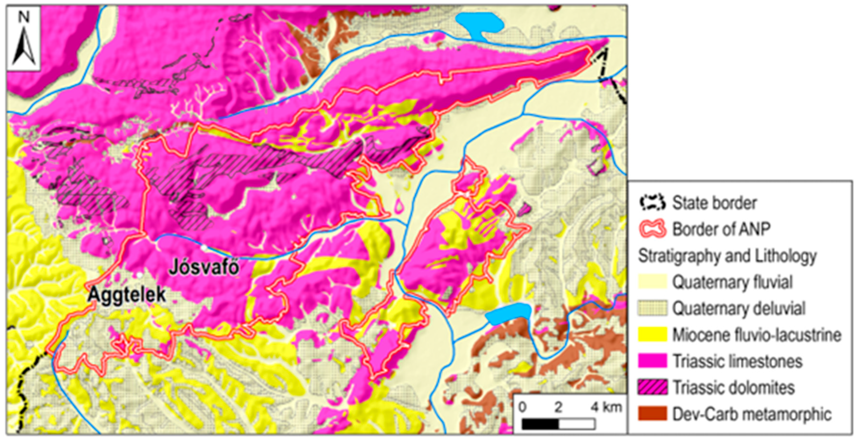
The lower Triassic strata, primarily clay slates and sandstones, function as aquicludes across an area of about 62 km², whereas the middle and upper Triassic formations consist of highly karstified limestones and dolomites spanning roughly 105 km². Smaller Miocene sand and gravel deposits are present in the southern parts, and Pliocene sediments (clay, sand, and gravel) cover around 35 km². A thin Pleistocene clayey soil layer, ranging from 0.2 to 1 m in thickness, blankets the plateau tops, while Holocene alluvial deposits, mainly gravel and sand, occupy the valley floors (Figure 5) [55].

Figure 5. Geological and tectonic settings of the Aggtelek Kkarst [56].

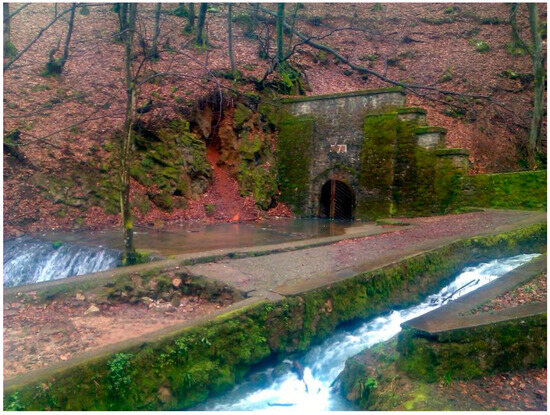
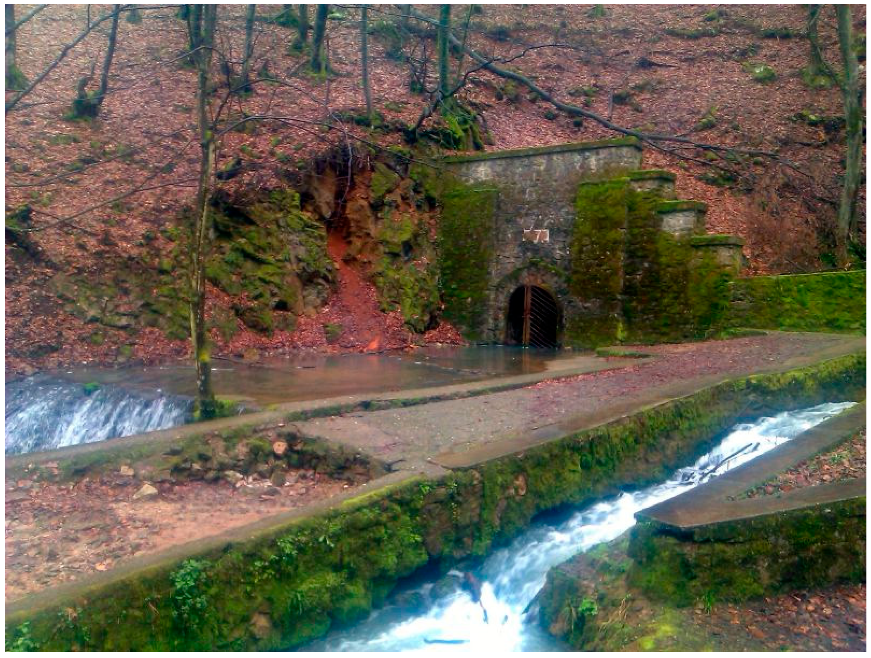
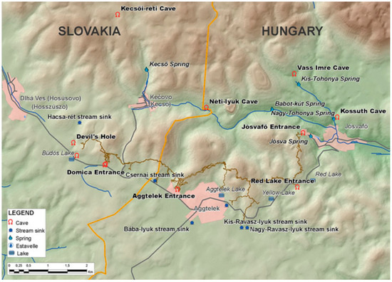
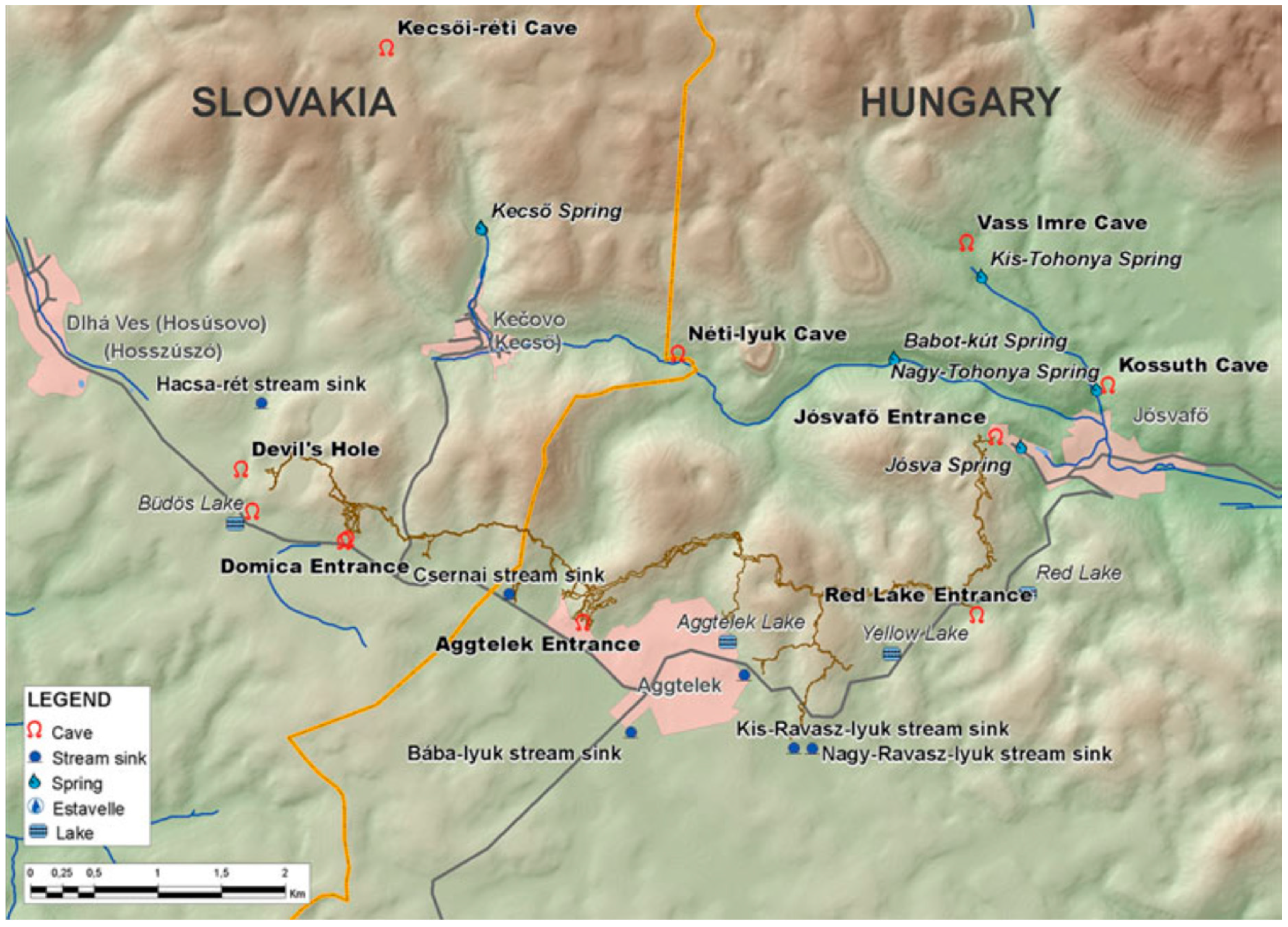
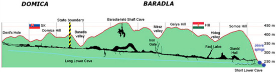
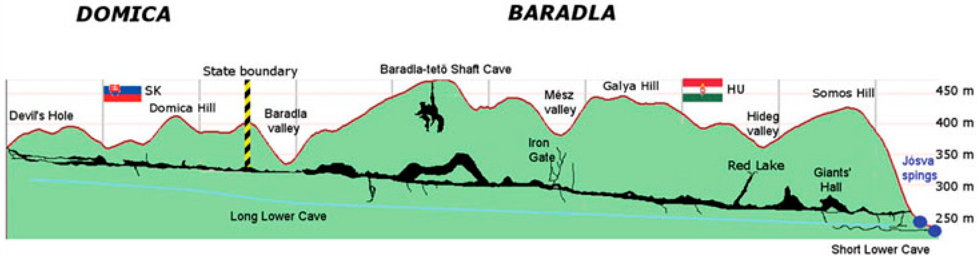
The Jósva spring (Figure 6), Hungary’s largest cold-water spring, is situated just west of the village of Jósvafő and comprises two distinct springs. The name “Jósva” refers to the karst water emerging from the lower galleries of the Baradla cave system (Figure 7 and Figure 8). The spring’s catchment covers about 34 km², part of which is only intermittently active due to surface coverage of the karst hills south of Aggtelek, causing recharge only during rainfall events. It is highly probable that water sinking in the Kecső Valley sinkholes also feeds into the Jósva spring system. Discharge rates vary widely, typically between 70 L/s and 8000 L/s, but reached a peak flow of 20,000 L/s in August 1955. The catchment borders Béke Cave to the east, Babot-kút and Tohonya Spring to the north, and extends well into Slovakia to the west (the Slovak section of Baradla is called Domica). The water temperature remains stable at around 10 °C.

Figure 6. The Jósva spring and the cave entrance.

Figure 7. Hydrological objects in the catchment area of Baradla–Domica cave system [54].

Figure 8. Location and longitudinal profile of Baradla–Domica cave system [54].

5. Simulating Discharge Peaks by Regression Analysis

Discharge peaks were simulated using classical regression analysis. Our primary objective was to develop a simple method that did not require a large number of climate parameters. This simplicity is vital, as many remote karst areas lack extensive historical datasets. However, rainfall data are generally easy to measure and widely available at most studied sites.

As a first step in the regression analysis, we tested various rainfall models, including different daily and multi-day cumulative rainfall approaches as well as methods for isolating peak discharges. The highest correlation was observed between peak discharge and the cumulative rainfall over two days. Consequently, regression analysis was conducted using two-day cumulative rainfall data.

Spring discharge is composed of two distinct components: quickflow and baseflow. Quickflow originates from concentrated recharge and responds directly to rainfall events, producing rapid increases in spring discharge. In contrast, baseflow arises from diffuse recharge and the delayed release of water stored within the rock matrix. Because of the slower, diffusive processes involved, baseflow exhibits a delayed response to rainfall compared to quickflow.

Given this dual nature of spring discharge, the initial step in our analysis was to establish correlations specifically between rainfall and the peaks in spring discharge. For this purpose, only the peak discharge values were considered in the regression analysis, while the baseflow component was treated separately and simulated using analytical modeling approaches.

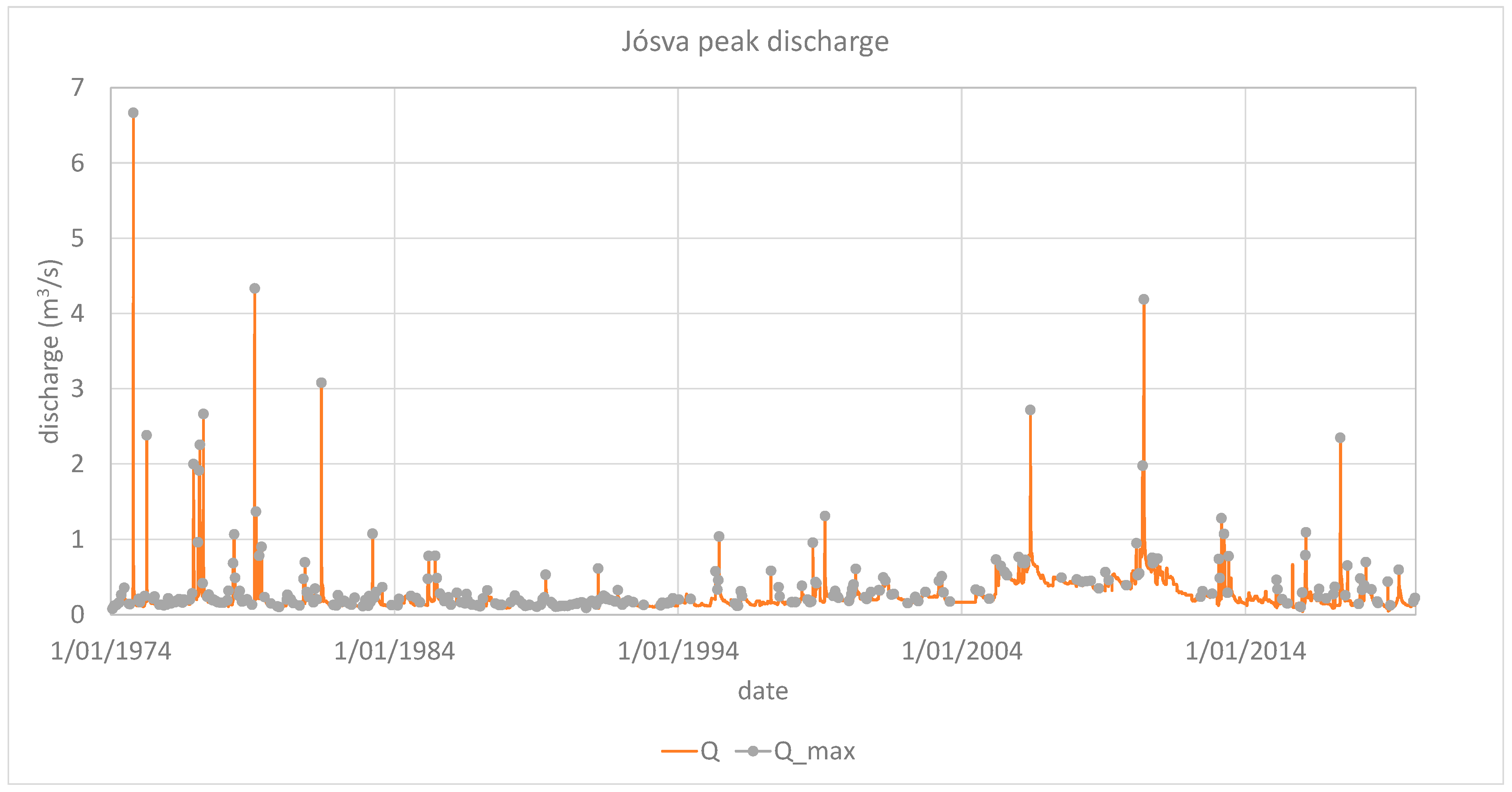
To accurately identify the discharge peaks, hydrograph segments were selected according to specific criteria. Segments were considered if they exhibited a minimum of two, five, or eight consecutive days of uninterrupted rising discharge, followed by an equivalent period of uninterrupted falling discharge. A comparison of these different selection criteria demonstrated that hydrograph segments preceded and followed by eight days of monotonic rising and falling discharge, respectively, provided the best match with the observed discharge peaks (Figure 9).

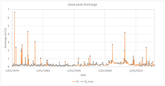
Figure 9. Measured spring hydrograph and discharge peak isolation, Jósva spring.

We put a large emphasis on model parsimony, and thus the simplest and most effective solution was always selected where it did not compromise the model fit. Although other models provided similar fit, we followed the “simplest is best” approach. The simplest and most effective solution was a simple linear model. Based on the temporal patterns observed in the discharge data, the most suitable regression function takes the general form shown in Equation (7) and illustrated in Figure 10.

$$Q_{max}=0.1789+0.0655·p_{cumul}$$

(7)

Figure 10. Regression model of peak discharge vs. rainfall.

Figure 10. Regression model of peak discharge vs. rainfall.

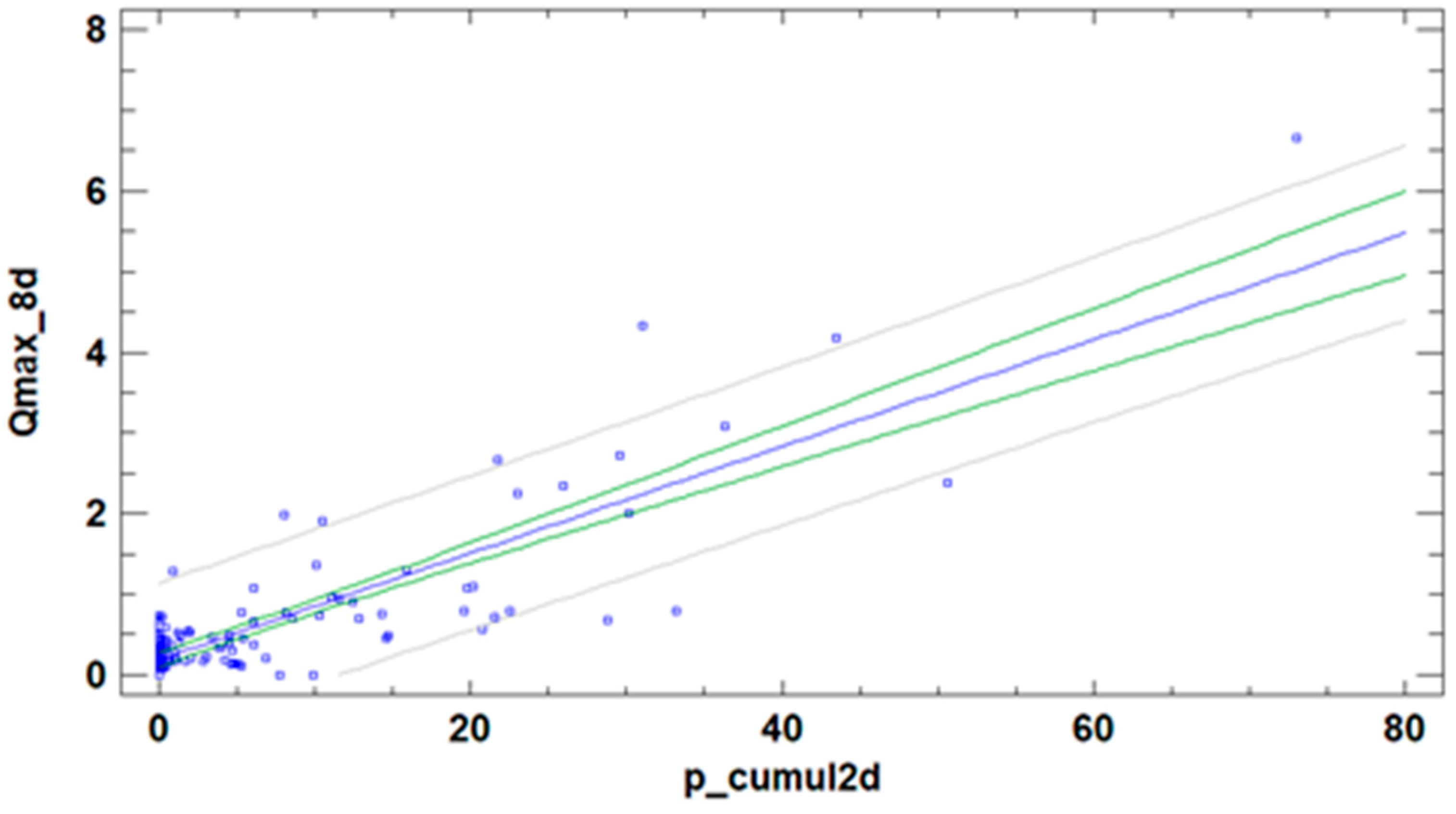
Here, Q_max represents the peak discharge (m³/s) and pcumul_2 denotes the two-day cumulative rainfall (mm).

The summary statistics for the regression model are provided in Table 2. The p-value obtained from the analysis of variance (ANOVA) was less than 0.05, indicating a statistically significant relationship between Q_max and pcumul_2 at the 95% confidence level. The R² value of 0.7090 suggests that the model explains approximately 70.9% of the variability in peak discharge.

Table 2. Summary statistics of simulated peak discharge vs. measured peak discharge.

Statistical Measure	Value
Correlation coefficient	0.84
R-squared	70.90%
Standard error of est.	0.46
Mean absolute error	0.26
Durbin–Watson statistic	1.65 (p = 0.0145)
Lag 1 residual autocorrelation	0.17

The correlation coefficient of 0.84 points to a moderately strong association between the variables. The standard error of the estimate, representing the standard deviation of the residuals, is 0.46, while the mean absolute error (MAE) of 0.26 reflects the average magnitude of the residuals. The Durbin–Watson (DW) statistic was calculated to test for serial correlation in the residuals based on their order in the data sequence. Since the DW test p-value was less than 0.05, this suggests the presence of possible serial correlation at the 95% confidence level.

6. Simulating Baseflow by Analytical Model

The baseflow of karst springs is primarily generated by the diffusive drainage of water from low-permeability matrix blocks [30]. Because this recession process occurs with a delay relative to rainfall events, conventional regression models linking rainfall and discharge are insufficient to accurately describe baseflow dynamics. Analytical modeling approaches are therefore more appropriate for capturing the behavior of baseflow.

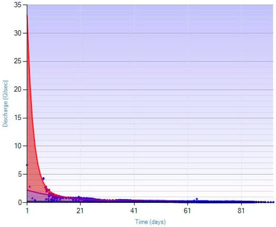
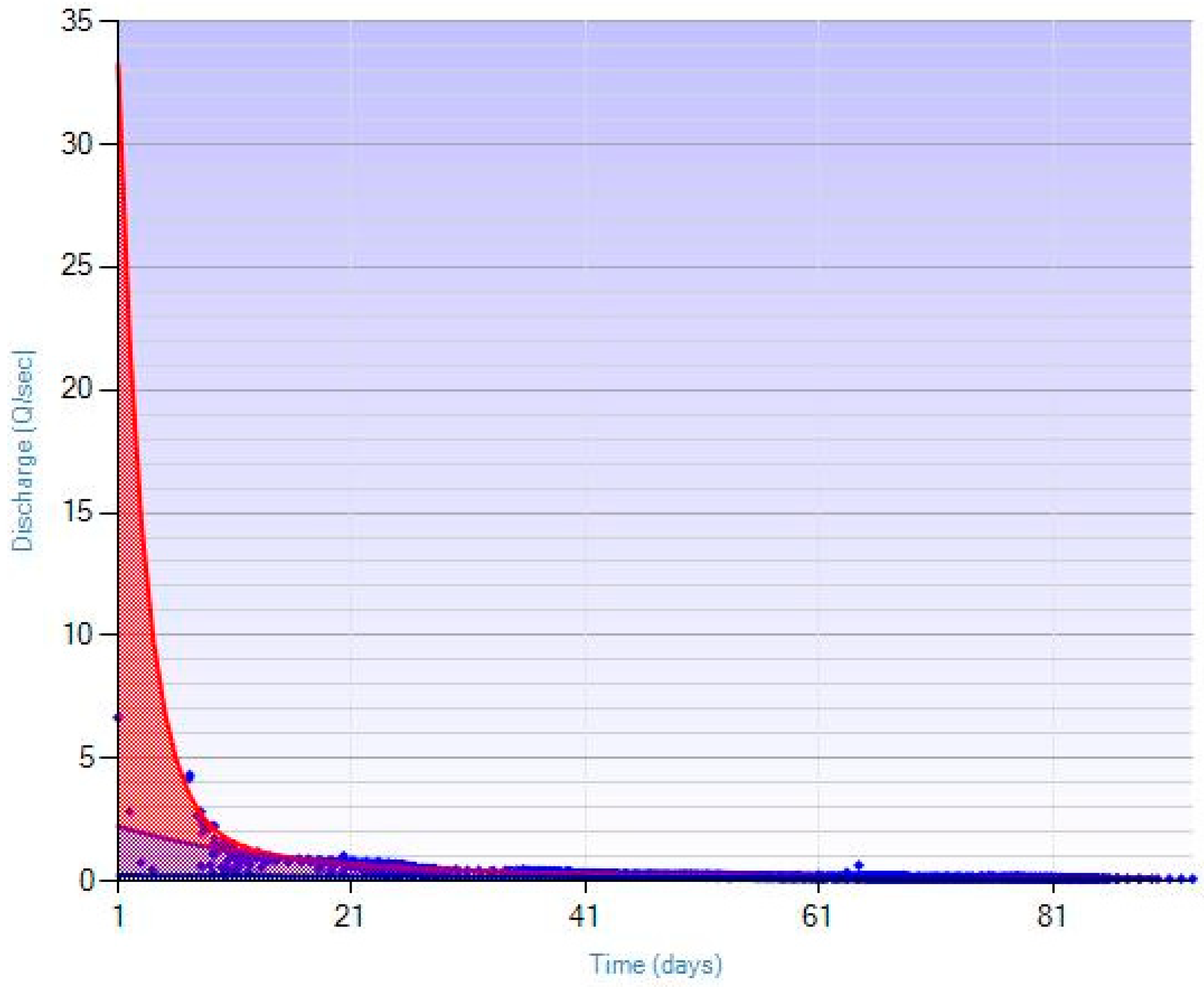
To create a simple, yet effective mathematical representation of baseflow at the Jósva spring, a master recession curve (MRC) was developed using the available discharge data. The MRC was constructed through the application of the hybrid genetic algorithm [57], a statistical search technique inspired by Darwinian evolutionary principles and categorized within artificial intelligence methods. The resulting MRC for the Jósva dataset is presented in Figure 11.

Figure 11. Master recession curve of the Jósva discharge time series and its decomposition.

Through curve fitting and decomposition of the master recession curve (MRC) for the Jósva hydrograph, the baseflow recession can be expressed mathematically using the following formula (Equation (8)):

$$Q_{\left(t\right)}=Q_{inf}{e}^{-0.002t}+Q_{inf}{e}^{-0.05t}$$

(8)

Here, Q_inf represents the inflexion point discharge calculated from discharge data using the regression function (Equation (9)):

$$Q_{inf}={0.251+0.0762lnQ}_{peak}$$

(9)

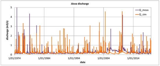
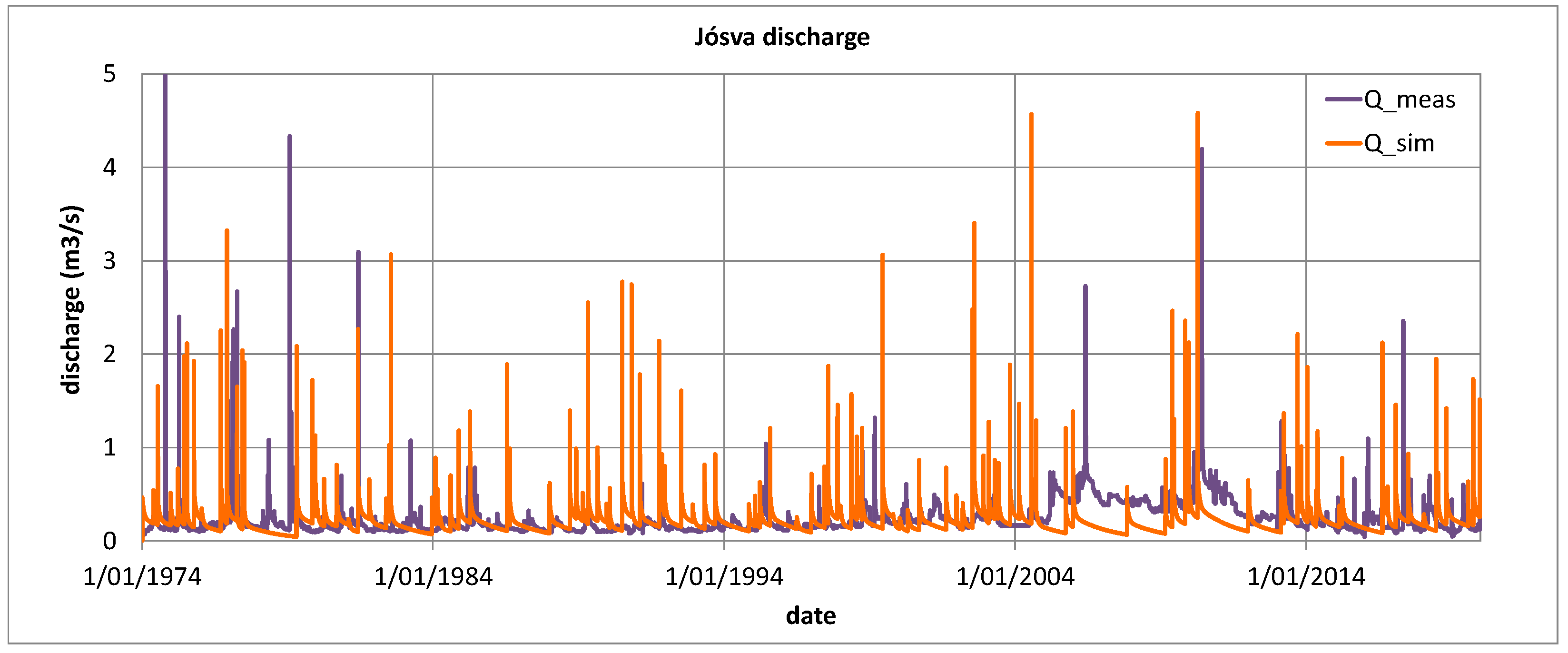
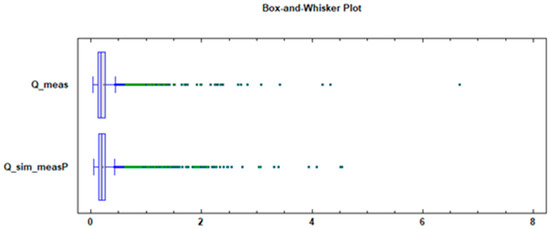
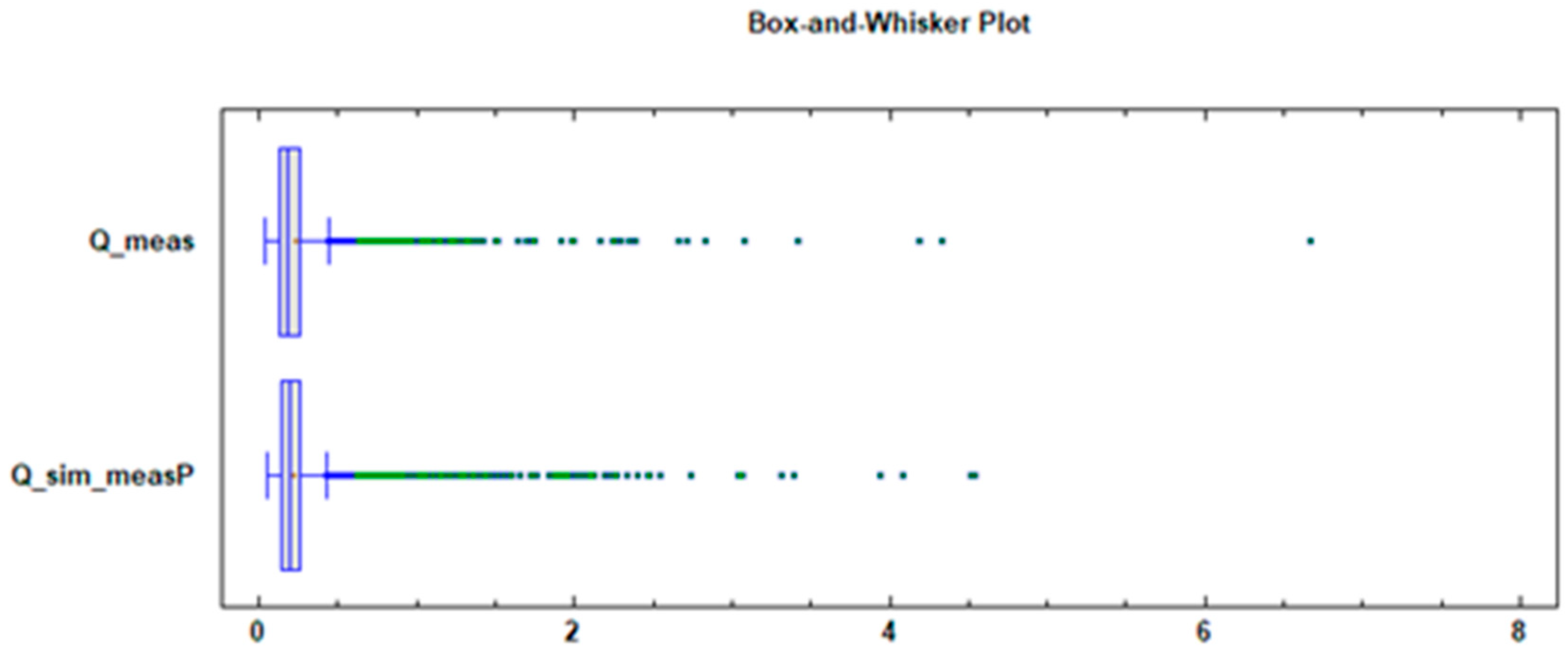
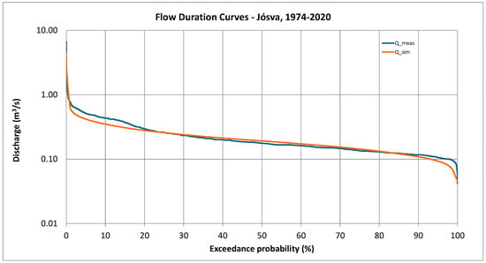
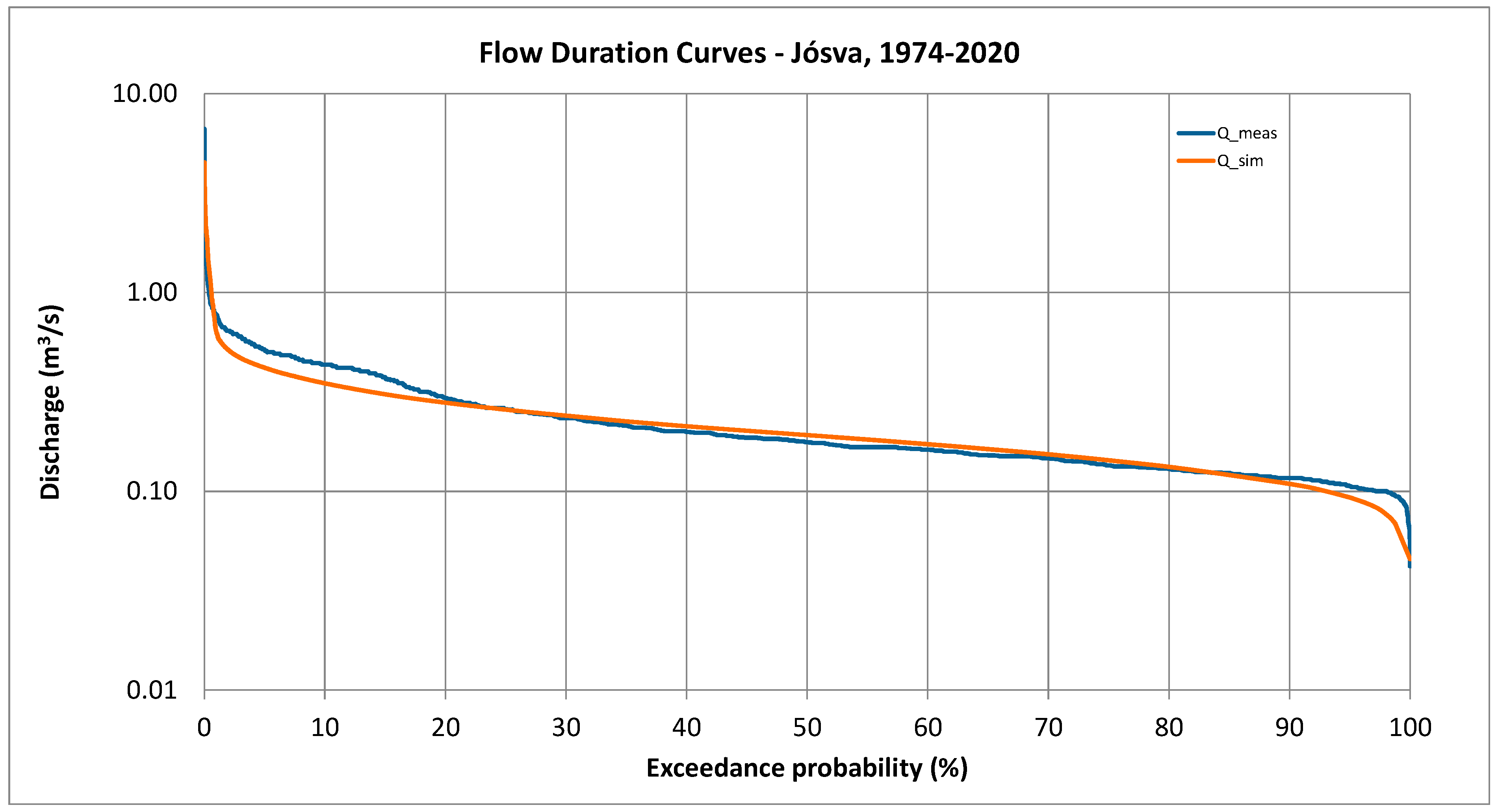
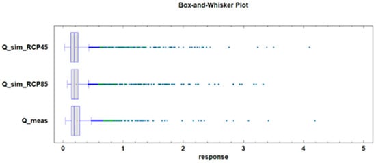
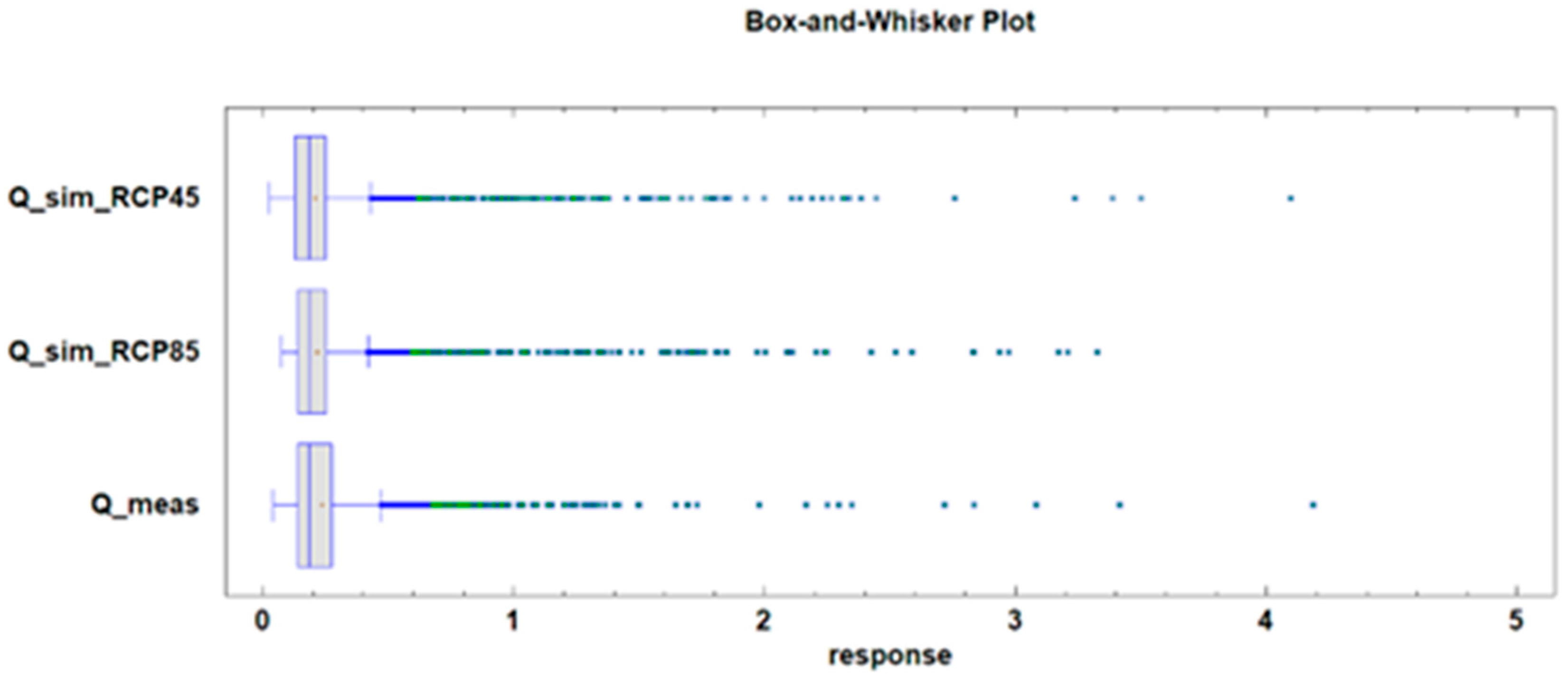
The simulated hydrograph is presented in Figure 12, and Figure 13 shows a box-and-whisker plot comparing the measured and simulated hydrographs. The comparison indicates minor deviations in the lower high-range and higher low-range discharges, yet the model provides an excellent fit for peak, mid-range, and baseflow discharges. Using the combined approach, complete hydrographs were reconstructed by integrating the regression function for peak discharge with the simplified analytical solution for baseflow. A statistical comparison between the observed discharge and the model outputs is summarized in Table 3. Furthermore, Figure 14 presents the flow duration curve for both measured and simulated data. The flow duration curve illustrates the percentage of time a specific discharge is equaled or exceeded over a given period, offering a graphical representation of the catchment’s hydraulic behavior under varying flow conditions. Overall, the combined model delivers a statistically robust estimate of measured discharge data, although some differences exist in the timing and magnitude of discharge peaks. These discrepancies likely arise because meteorological data do not always fully capture spatial or temporal rainfall variability across the catchment. The model also slightly underestimates lower high-range and higher low-range discharges, though these differences are minor. In summary, the model effectively estimates spring discharge, which remained the main objective of this study.

Figure 12. Comparison between measured and simulated hydrographs based on measured rainfall data.

Figure 13. Box-and-whisker plot of measured and simulated spring hydrographs.

Table 3. Summarized statistics of applied models.

	Q_meas_(m3/s)	Q_sim_(m3/s)
Count	16,801	16,799
Average	0.23	0.22
Standard deviation	0.17	0.17
Coeff. of variation	75.82%	75.83%
Minimum	0.042	0.045
Maximum	6.67	4.54
Range	6.62	4.49
Stnd. skewness	438.03	495.41
Stnd. kurtosis	4815.15	4065.74

Figure 14. Comparison of flow duration curves of the measured and simulated spring hydrographs.

Model performance was evaluated using the Nash–Sutcliffe efficiency (NSE), mean absolute relative error (MARE), and root mean square error (RMSE). The model’s performance varies due to measurement errors and data uncertainties, particularly during the 2004–2014 period. Overall, the model demonstrates good performance, as reflected by the calculated statistics: NSE = 0.7122, MARE = 1.89%, and RMSE = 0.00396.

7. Comparison of Measured vs. Projected Discharge (1981–2000)

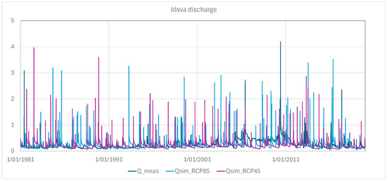
Predictions of peak discharge at the Jósva spring were obtained using the previously described simple linear regression model (Equation (7)), while baseflow was simulated with the analytical model (Equation (8)). Discharge time series were generated using rainfall projections from regional climate models (RCMs) for three time periods: 1981–2020, 2021–2060, and 2061–2100. For each period, computations were performed under the two RCM scenarios listed in Table 1, enabling a comparative assessment of scenario-based discharge statistics over time. As noted earlier, these predicted discharge patterns reflect the outputs of downscaled climate models and thus carry the inherent uncertainties and assumptions of those models.

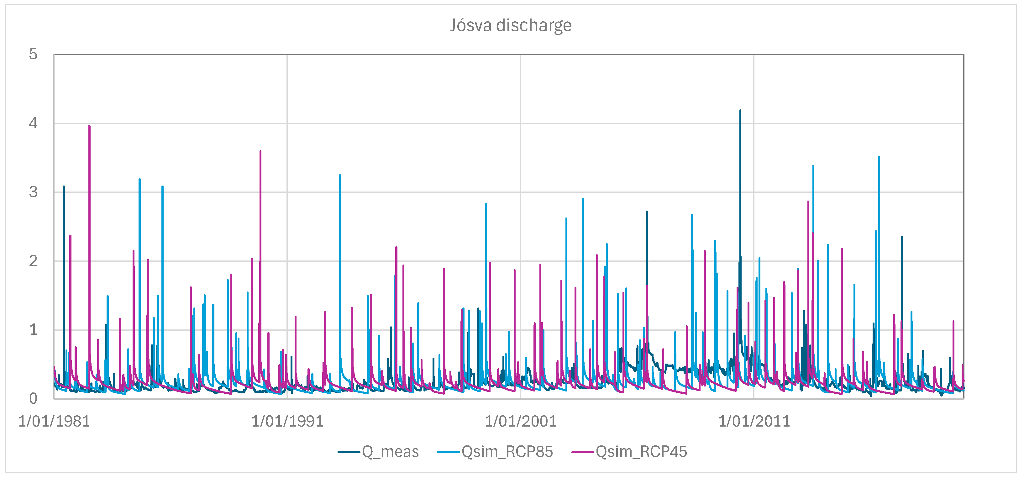
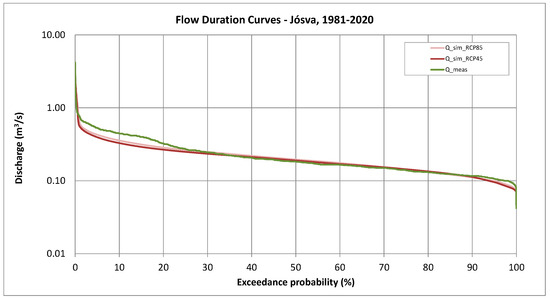
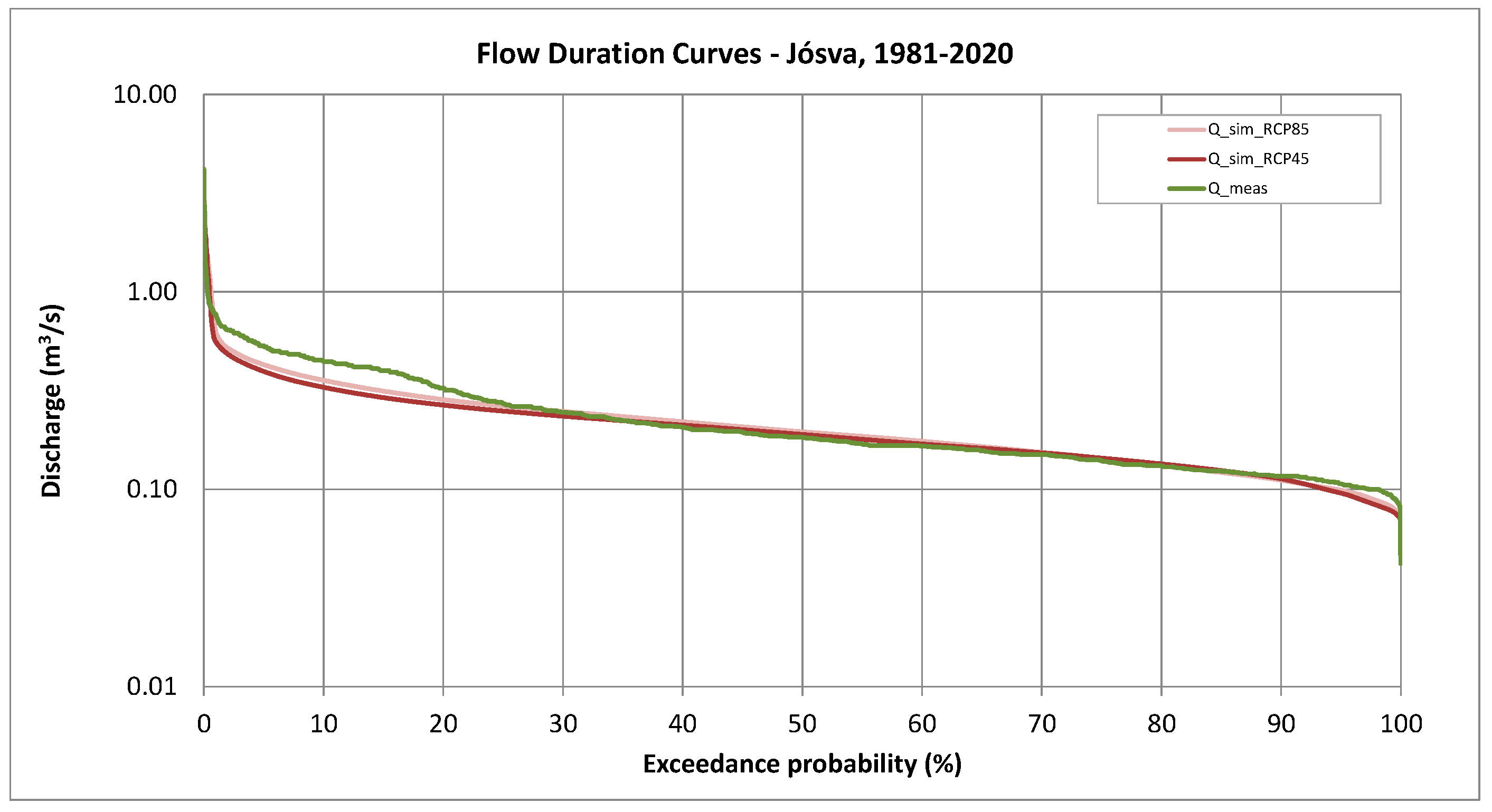
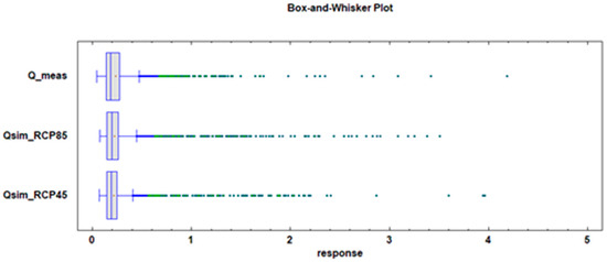
The predicted discharge time series for 1981–2020 are shown in Figure 15, along with the corresponding flow duration curves for the different scenarios (Figure 16). Summary statistics for these predictions are provided in Table 4, and the associated box-and-whisker plots are presented in Figure 17. Comparison of Figure 16 and Figure 17, together with the data in Table 4, indicates that the model tends to slightly underestimate peak discharges while slightly overestimating minimum flows. Despite these minor deviations, the flow duration curves in Figure 16 show that the modeled discharge reasonably approximates the observed hydrograph.

Figure 15. Forecast spring hydrographs for the period 1981–2020. Discharge was calculated from RCM projections using the combined statistical–analytical model.

Figure 16. Comparison of flow duration curves of the measured and predicted spring hydrographs for the 1981–2020 period.

Table 4. Summary statistics of multiple-sample comparison amongst predicted and measured spring hydrographs.

	Count	Average	Standard Deviation	Coeff. of Variation	Minimum	Maximum
Q_meas	14,241.00	0.24	0.17	0.69	0.04	4.19
Q_sim_RCP85	14,972.00	0.23	0.16	0.72	0.07	3.51
Q_sim_RCP45	14,972.00	0.21	0.14	0.67	0.07	3.96
Total	44,185.00	0.23	0.16	0.70	0.04	4.19

Figure 17. Box-and-whisker plot of measured and projected spring discharge (1981–2020).

8. Discharge Predictions

The central goal of this research was to project the discharge of karst springs using rainfall data derived from regional climate model (RCM) outputs, with the aim of assessing how climate change may influence spring hydrology. Predictions were made for two forthcoming 40-year intervals: 2021–2060 and 2061–2100. For this purpose, a bias-corrected, integrated statistical–analytical modeling approach was utilized, enabling the estimation of future spring discharge under RCM-generated rainfall scenarios.

8.1. Predictive Simulations for 2021–2060

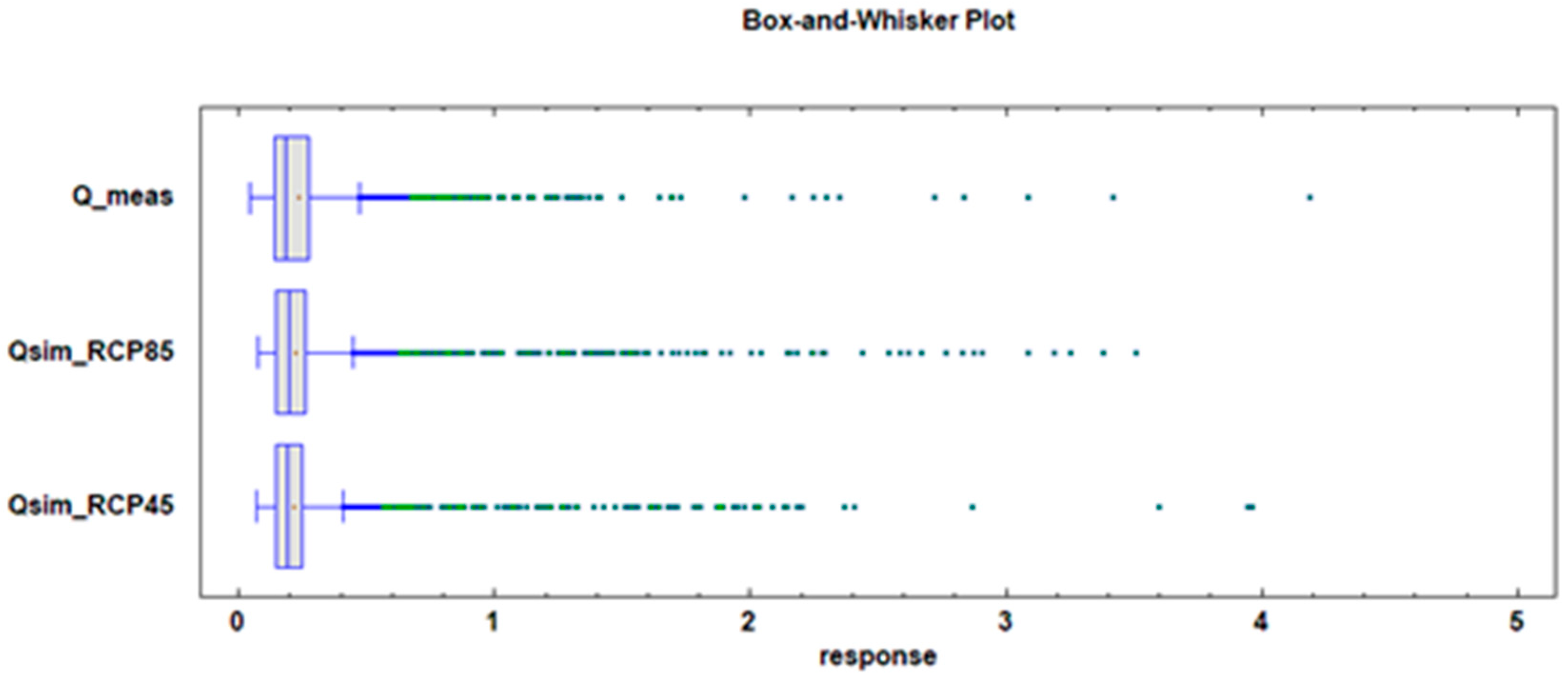
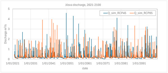
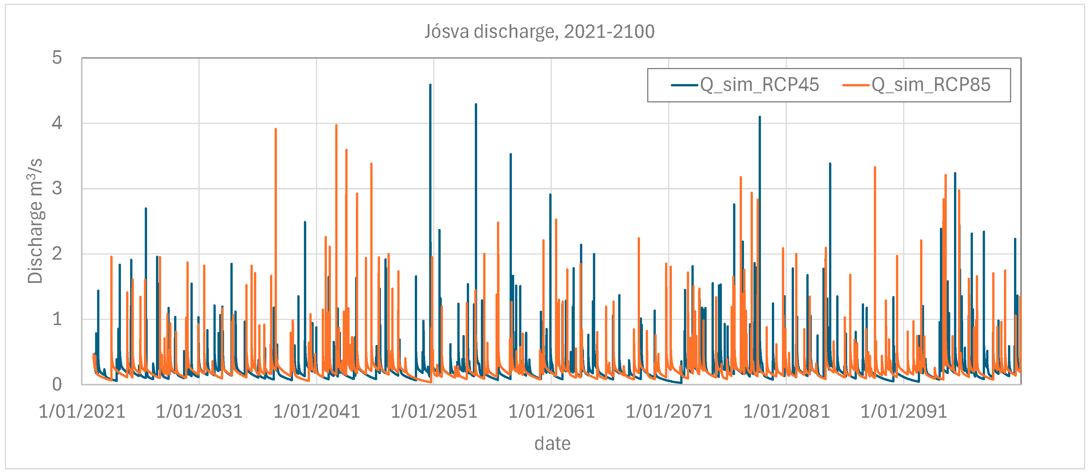
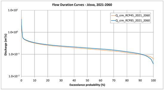
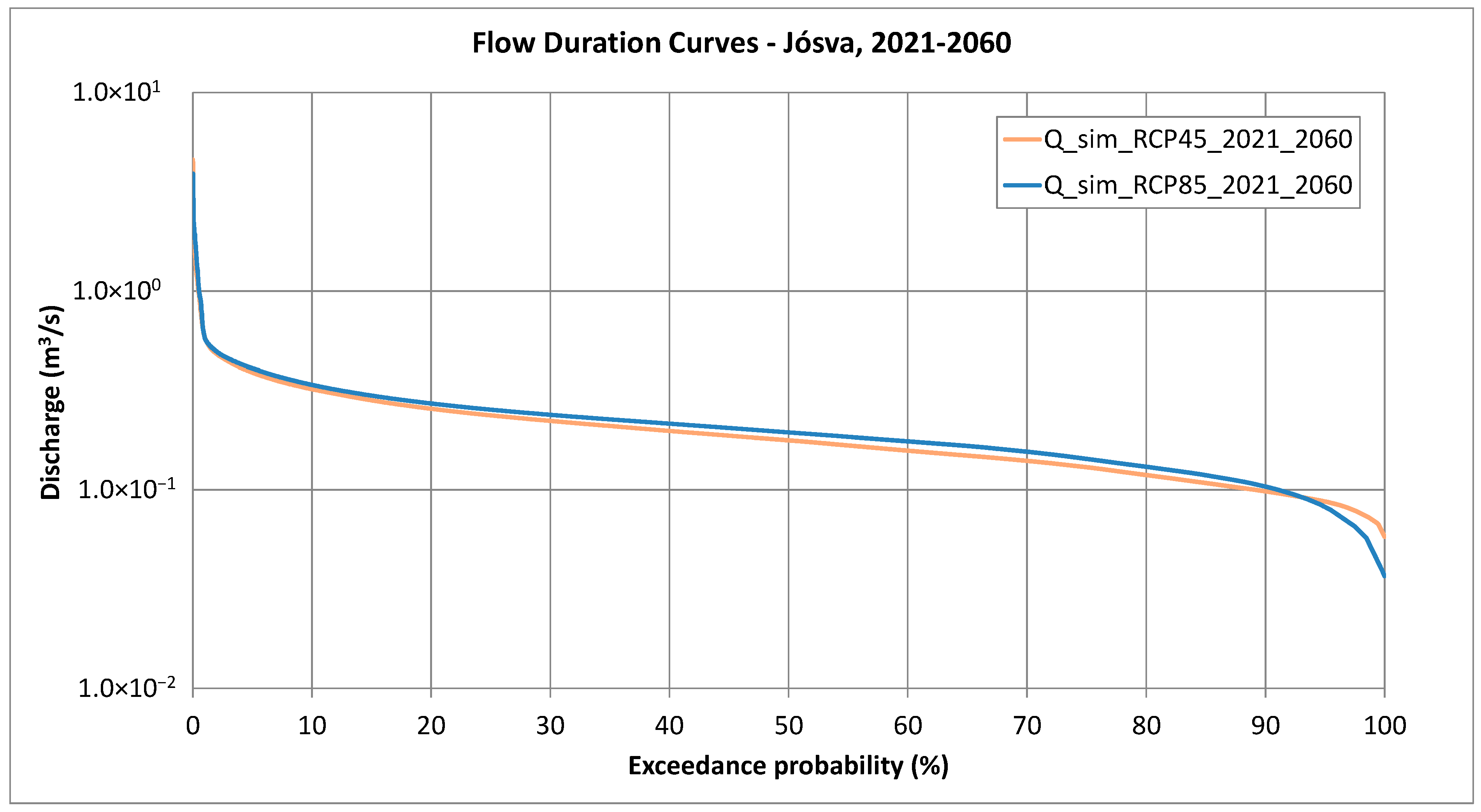
The projected spring hydrographs obtained from RCM Scenario 1 and Scenario 2 are illustrated in Figure 18, while the associated flow duration curves are shown in Figure 19 and the box-and-whisker plot is presented in Figure 20. Summary statistics for the simulations are compiled in Table 5. A comparison of the two scenarios for the 2021–2060 period reveals that Scenario 1 produces both higher peak discharges and higher baseflow values compared to Scenario 2. Despite these differences, the mean discharge values remain largely similar between the two scenarios.

Figure 18. Spring hydrograph forecasts for the 2021–2100 period based on RCMs.

Figure 19. Flow duration curves of spring discharge forecasts for the 2021–2050 period based on RCMs. The bias-corrected combined statistical–analytical model was applied.

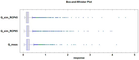
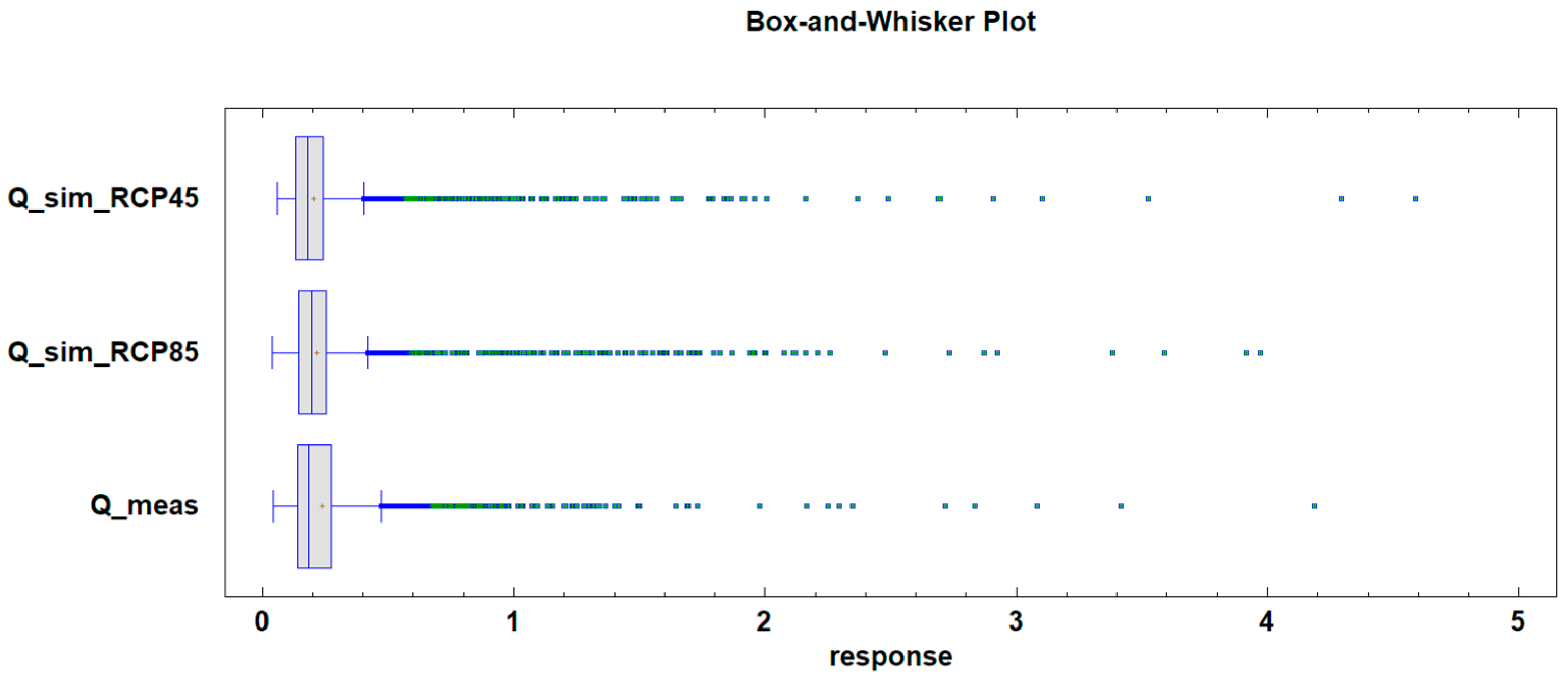
Figure 20. Box-and-whisker plot of predicted bias-corrected spring discharge for the 2021–2060 period based on RCMs. Measured data from 1981–2020 included for comparison.

Table 5. Summary statistics of predicted and measured spring hydrographs for the 2021–2060 simulation period. Measured data from 1981–2020 included for comparison.

	Q_sim_RCP45	Q_sim_RCP85	Q_meas
Count	14,242	14,242	14,244
Average	0.21	0.22	0.24
Standard deviation	0.15	0.16	0.17
Coeff. of variation	0.72	0.71	0.69
Minimum	0.06	0.04	0.04
Maximum	4.59	3.97	4.19
Range	4.53	3.94	4.15
Stnd. skewness	450.43	411.66	246.29
Stnd. kurtosis	4173.40	3174.14	1662.77

8.2. Predictive Simulations for 2061–2100

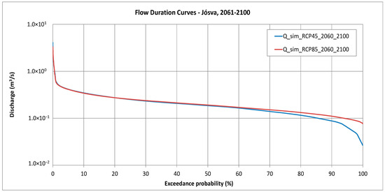
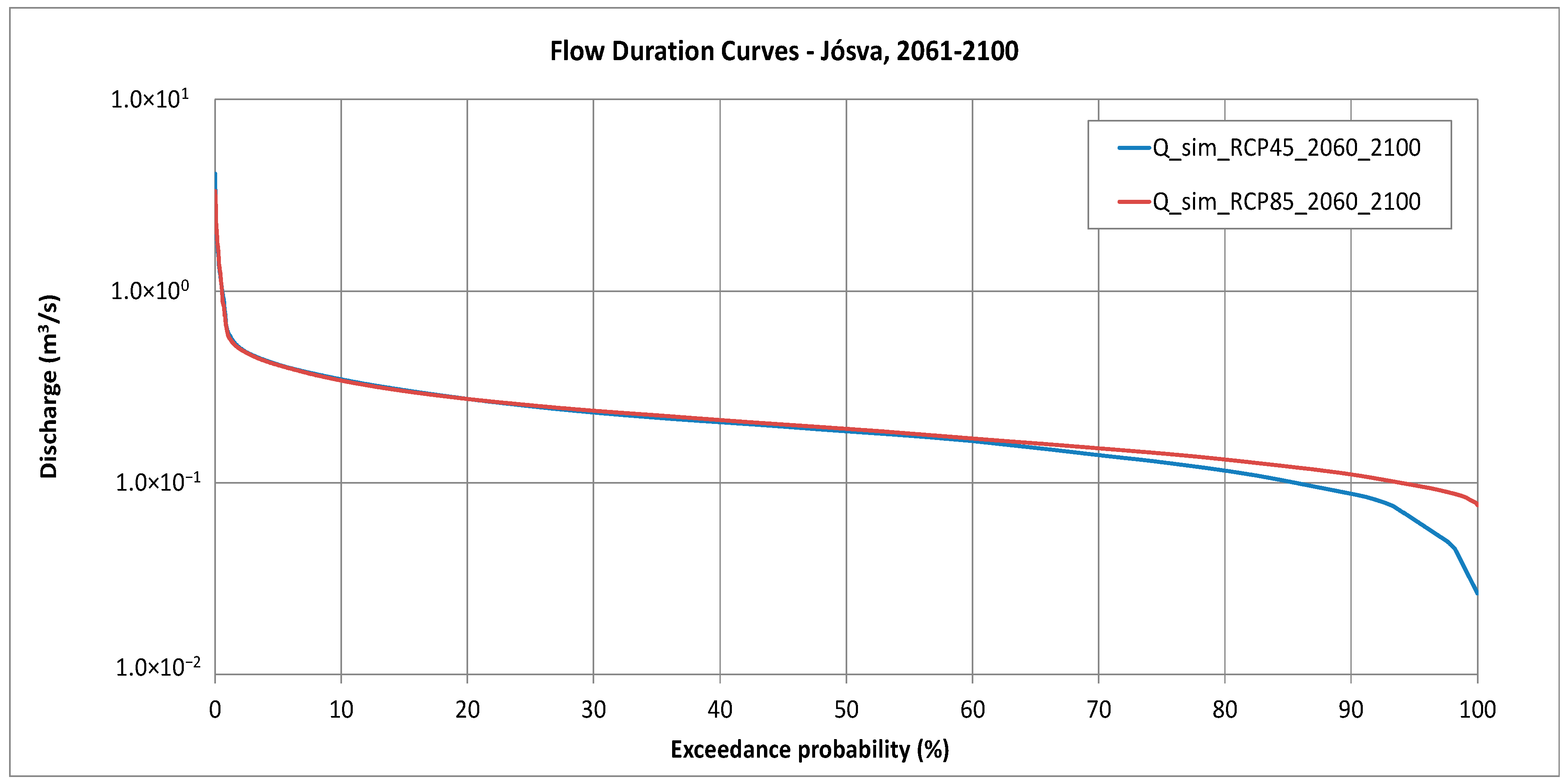
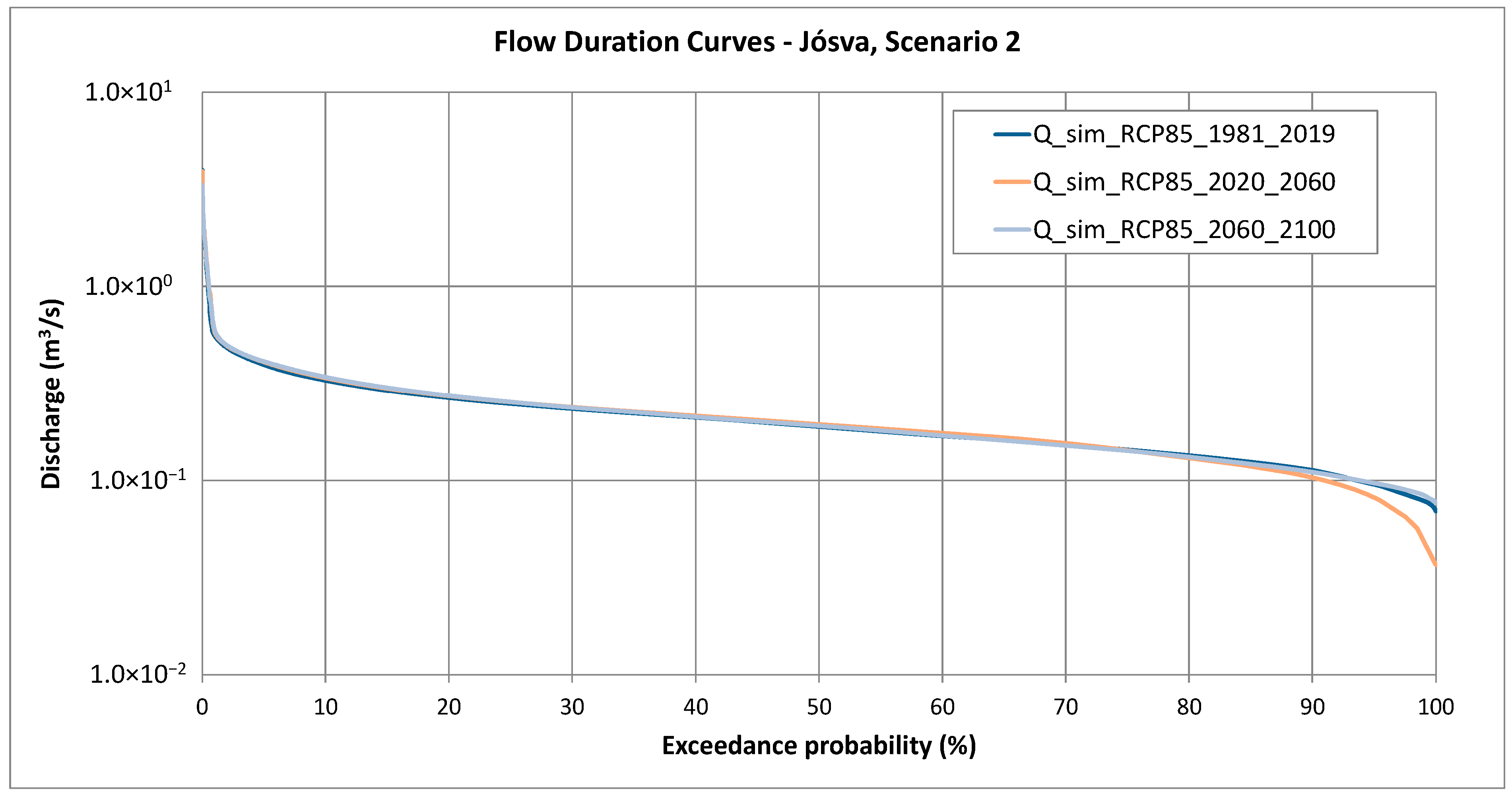
The projected spring hydrographs for the 2061–2100 simulation period, based on RCM Scenario 1 and Scenario 2, are shown in Figure 19. The associated flow duration curves are illustrated in Figure 21, and the box-and-whisker plot is presented in Figure 22. A summary of the statistics is provided in Table 6. A comparison of the two scenarios indicates that Scenario 1 produces higher peak discharges, but lower baseflow discharges than Scenario 2. Despite these differences, the average discharge is similar between the two scenarios.

Figure 21. Flow duration curves of spring discharge forecasts for the 2071–2100 period based on RCMs. The bias-corrected combined statistical–analytical model was applied.

Figure 22. Box-and-whisker plot of predicted bias-corrected spring discharge for the 2061–2100 period based on RCMs. Measured data from 1981–2020 included for comparison.

Table 6. Summary statistics of bias-corrected predicted and measured spring hydrographs for the 2071–2100 simulation period. Measured data from 1981–2020 included for comparison.

	Q_sim_RCP45	Q_sim_RCP85	Q_meas
Count	14,609	14,609	14,244
Average	0.21	0.22	0.24
Standard deviation	0.16	0.15	0.17
Coeff. of variation	0.75	0.70	0.69
Minimum	0.03	0.08	0.04
Maximum	4.10	3.33	4.19
Range	4.07	3.25	4.15
Stnd. skewness	361.45	393.99	246.29
Stnd. kurtosis	2616.29	2711.04	1662.77

9. Discussion

A regression relationship between rainfall and peak discharge was developed based on historical data spanning 1974 to 2020. The baseflow recession was represented using a two-component exponential model, with hydrograph decomposition and parameter calibration performed on the master recession curve (MRC). Future spring discharge was predicted using rainfall time series from two selected regional climate model (RCM) scenarios, with simulations carried out for three periods: 1981–2020, 2021–2060, and 2061–2100.

9.1. Flowrate Statistics

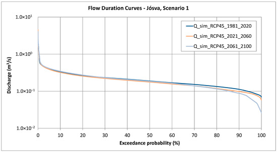
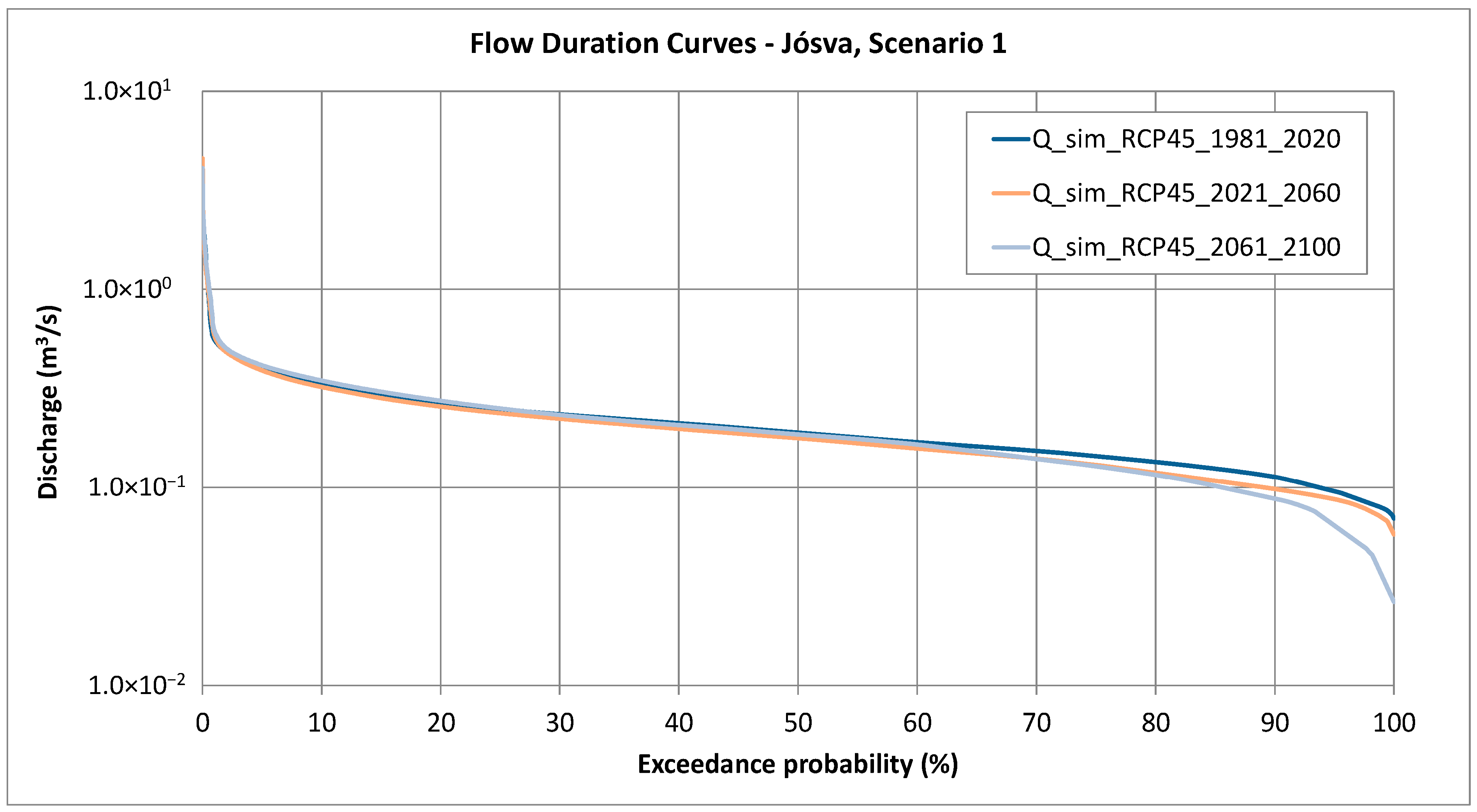
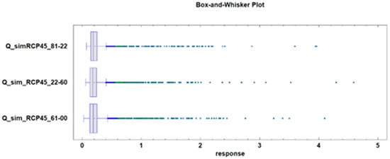
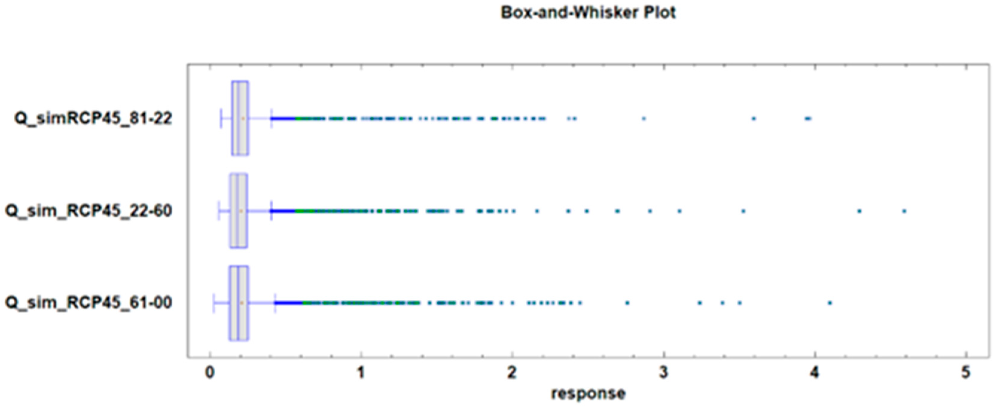
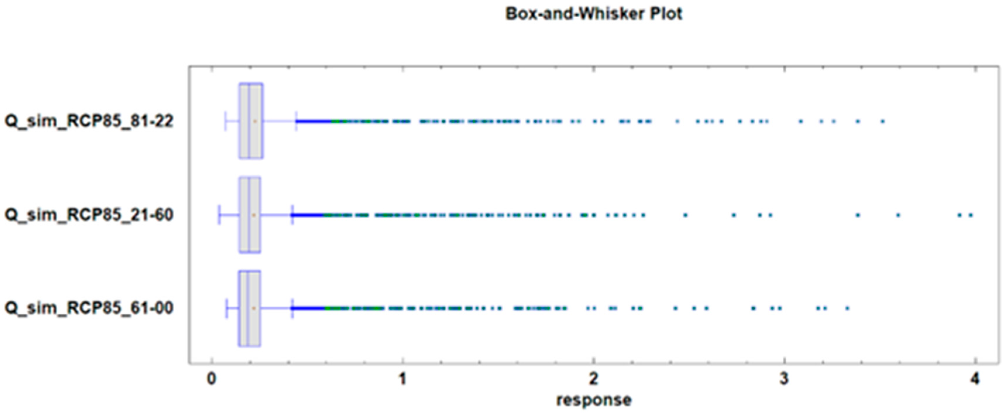
• The summary statistics presented in Table 7, along with the hydrograph of the Scenario 1 predictive models shown in Figure 23, and the Box-and-whisker plot shown in Figure 24 highlight the following observed trends: peak discharge increases significantly during the first half of the 21st century and decreases in the second half, although it remains higher than the current baseline.
• Average discharge shows little variation and remains relatively stable throughout the century.
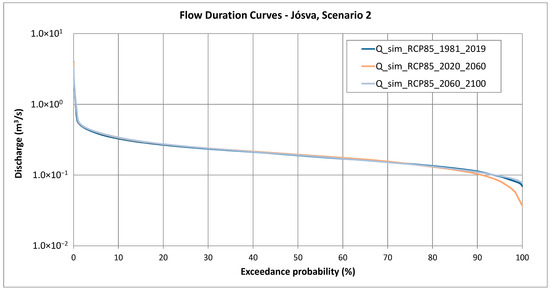
• Baseflow discharge exhibits a notable decline during the second half of the century.
• Likewise, the summary statistics in Table 8, together with the flow duration curve shown in Figure 25 and the box-and-whisker plot in Figure 26, indicate that peak discharge rises in the first half of the 21st century, but declines in the latter half.
• Average discharge remains nearly constant over the entire century.
• Baseflow discharge decreases during the first half of the century, followed by an increase in the second half, surpassing present-day values.

Table 7. Summary statistics of Scenario 1 predicted and measured spring hydrographs for the 1981–2020, 2021–2060, and 2061–2100 simulation periods.

	Q_sim_RCP45_81-22	Q_sim_RCP45_22-60	Q_sim_RCP45_61-00
Count	14,972	14,242	14,609
Average	0.21	0.21	0.21
Standard deviation	0.14	0.15	0.16
Coeff. of variation	0.67	0.72	0.75
Minimum	0.07	0.06	0.03
Maximum	3.96	4.59	4.10
Range	3.89	4.53	4.07
Stnd. skewness	438.35	450.43	361.45
Stnd. kurtosis	3543.28	4173.40	2616.29

Figure 23. Flow duration curves of spring discharge forecasts for the 1981–2020, 2021–2060, and 2061–2100 periods based on Scenario 1 RCM projection.

Figure 24. Box-and-whisker plot for the 1981–2020, 2021–2060, and 2061–2100 periods based on Scenario 1 RCM projection.

Table 8. Summary statistics of Scenario 2 bias-corrected predicted spring hydrographs for the 2008–2010, 2021–2050, and 2071–2100 simulation periods.

	Q_sim_RCP85_81-22	Q_sim_RCP85_21-60	Q_sim_RCP85_61-00
Count	14,972	14,242	14,609
Average	0.23	0.22	0.22
Standard deviation	0.16	0.16	0.15
Coeff. of variation	0.72	0.71	0.70
Minimum	0.07	0.04	0.08
Maximum	3.51	3.97	3.33
Range	3.44	3.94	3.25
Stnd. skewness	390.09	411.66	393.99
Stnd. kurtosis	2601.58	3174.14	2711.04

Figure 25. Flow duration curves of spring discharge forecasts for the 1981–2020, 2021–2060, and 2061–2100 periods based on Scenario 2 RCM projection.

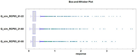
Figure 26. Box-and-whisker plot for the 1981–2020, 2021–2060, and 2061–2100 periods based on Scenario 2 RCM projection.

9.2. Spectral Analysis

To identify periodicities in the data, both spectral analysis using the discrete Fourier transform [58,59] and wavelet analysis [60] were employed. With the two methods combined, we were able to detect several cycles and evaluate of their significance inside the examined time interval. The results from the spectral analysis can be found in Table 9. Because the datasets present different time intervals, in several cases longer cycles have been defined. By examining the results together, it can be said that from annual data the cycles around 5-year long have the largest amplitudes, and from monthly data the presence of a strong annual cycle was detected amongst others. From the two forecast datasets, several similar periods were obtained, meaning the cyclicity of these RCMs is closely related.

Table 9. The results of the spectral analysis.

Discharge (m3/s)	Periods from Annual Data (yr)	Periods from Monthly Data (Month)
Measured discharge (m3/s), 1974–2020	2.9, 2.4, 2.8, 3.7, 4.8, 6.8, 12	2.10, 3.92, 4.03, 4.18, 4.55, 5.27, 9.56, 10.07, 11.28, 12, 13.76, 15.24, 18.8, 23.5, 29.68, 43.38, 56.4, 141
Scenario 1 discharge (m3/s), 1981–2100	2.2, 2.4, 2.5, 2.9, 3.25, 3.4, 3.7, 4.6, 5.5, 7, 10, 24, 40	2.15, 2.66, 2.91, 3.2, 3.4, 4.06, 4.4, 4.9, 5.6–5.8, 6, 7.1, 7.6, 9.29, 10.2, 10.6, 12, 12.6, 13.7, 14.5, 16, 17.7, 18.9, 20.5, 24, 26.6, 30, 35.1, 41.1, 45, 55.3, 84.7, 120, 205.7, 288
Scenario 2 discharge (m3/s), 1981–2100	2.1, 2.4, 2.6, 3, 3.5, 4.3, 4.8, 5.2, 5.7, 8, 10, 12, 15, 30	2.2, 2.6–2.7, 3.6, 4, 4.7, 5.3, 6.1,6.4, 8, 8.6, 9.5, 11, 12, 13.8, 15.1, 16,19.5, 24.4, 30.6, 42.3, 51.4, 57.6, 62.2, 96, 180, 360

9.3. Wavelet Analysis

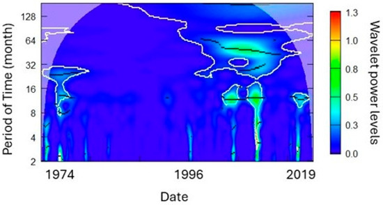
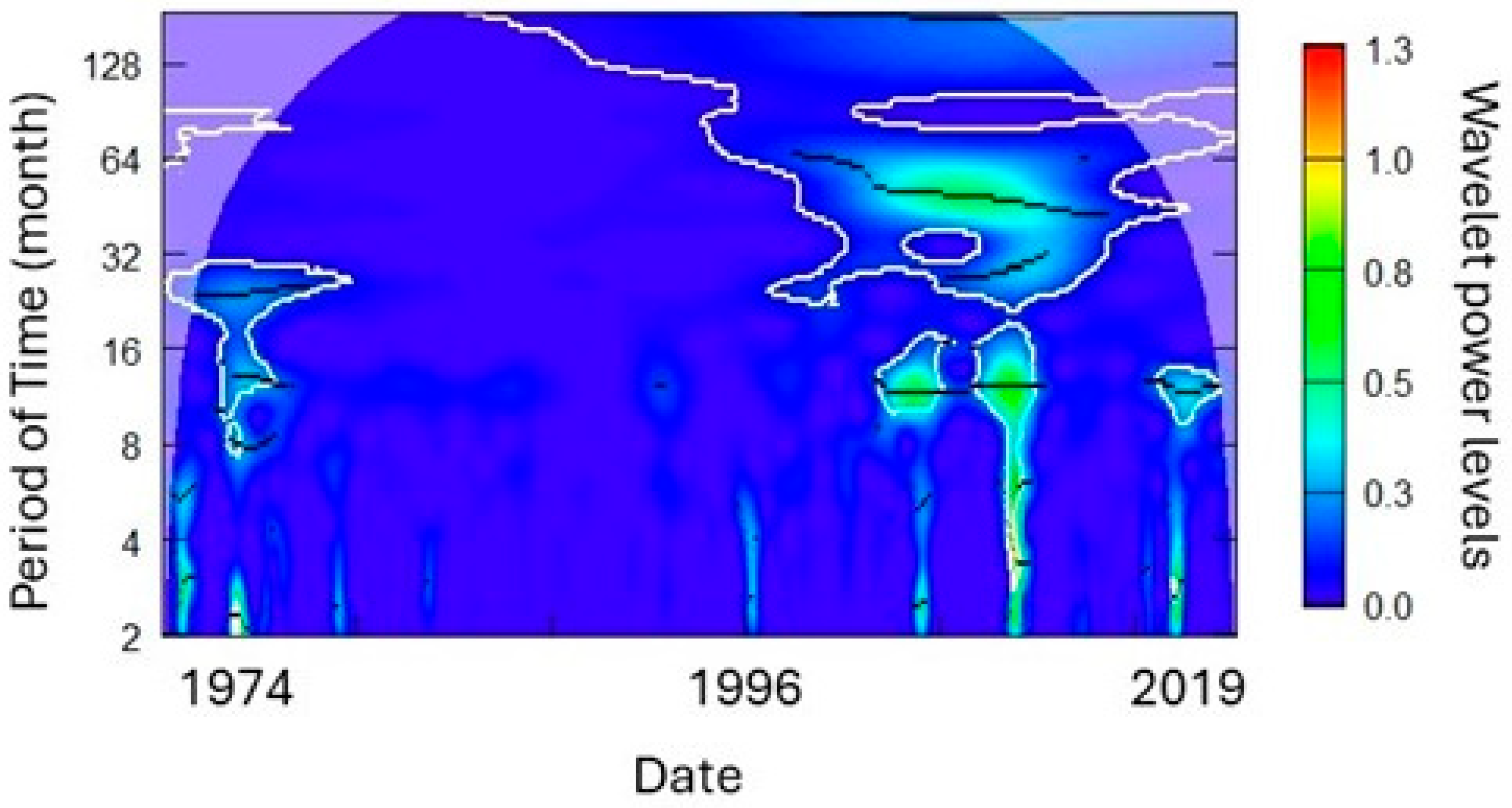
With the help of wavelet analysis, we were able to define which of these cycles detected by the spectral analysis were significant (Figure 27). In the original measured dataset from annual measurements, a 3.7-year cycle can be calculated, but this was not significant. From monthly values, cycles of 12, 23.5, and 56.4 months are all significant at a 0.05 level. From the simulated discharge data, only the 4.8-year cycle is significant. When considering monthly data, the 18- and 43-month cycles are significant, with less significant peaks at 12 and 6 months.

Figure 27. Wavelet of the monthly measured discharge data of the Jósva spring.

The simulated datasets cover a larger time period, and thus longer cycles can be detected. In Scenario 1 simulated data, the 2.4-year cycle has the largest wavelet power, but not significantly. Only the 12-year and 24-year cycles fulfill the criteria. From monthly values, the 1-year cycle has a strong presence in the dataset with 32-, 96-, and 128-month cycles being equally significant. In the Scenario 2 annual dataset, 2.6- to 2.7-, 4.7-, 8.6-, 16-, and 32-year cycles are present, with the latter two being significant. From monthly data the largest power occurs at 5.5 months, with significant maximums at 12, 30.6, 62.2, 96, 180 and 360 months.

By examining the four datasets together, we can detect similarities between them. All the four wavelets have a strong period at around 2 and 4 years, most not significant. In three cases, a period at around 8 years is visible also, with the two long-term forecast containing longer cyclic similarities. The two wavelets examining the 1974–2020 period have similarities in their cycles at around 6-, 12-, and 24-month periods. The two wavelets examining the forecast data share large similarity. The results correspond with the findings of previous studies examining precipitation in the area [58,59], showing a strong effect of rainfall pattern on the karst water yields. These periodicities have practical value for long-term prediction. The 6- to 9-year drought cycle observed in the data helps to explain discharge variability beyond simple rainfall–discharge relationships, especially for delayed baseflow responses. Recognizing these cycles also supports early warning of extreme hydrological years, enabling better drought risk anticipation and resource management.

9.4. Extreme Events

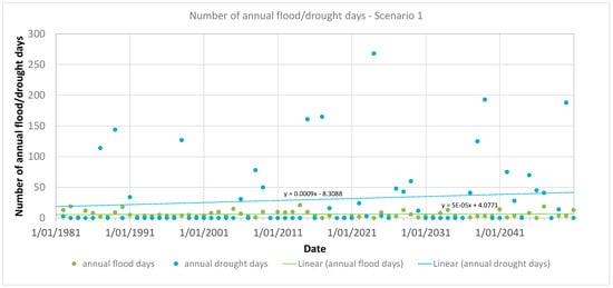
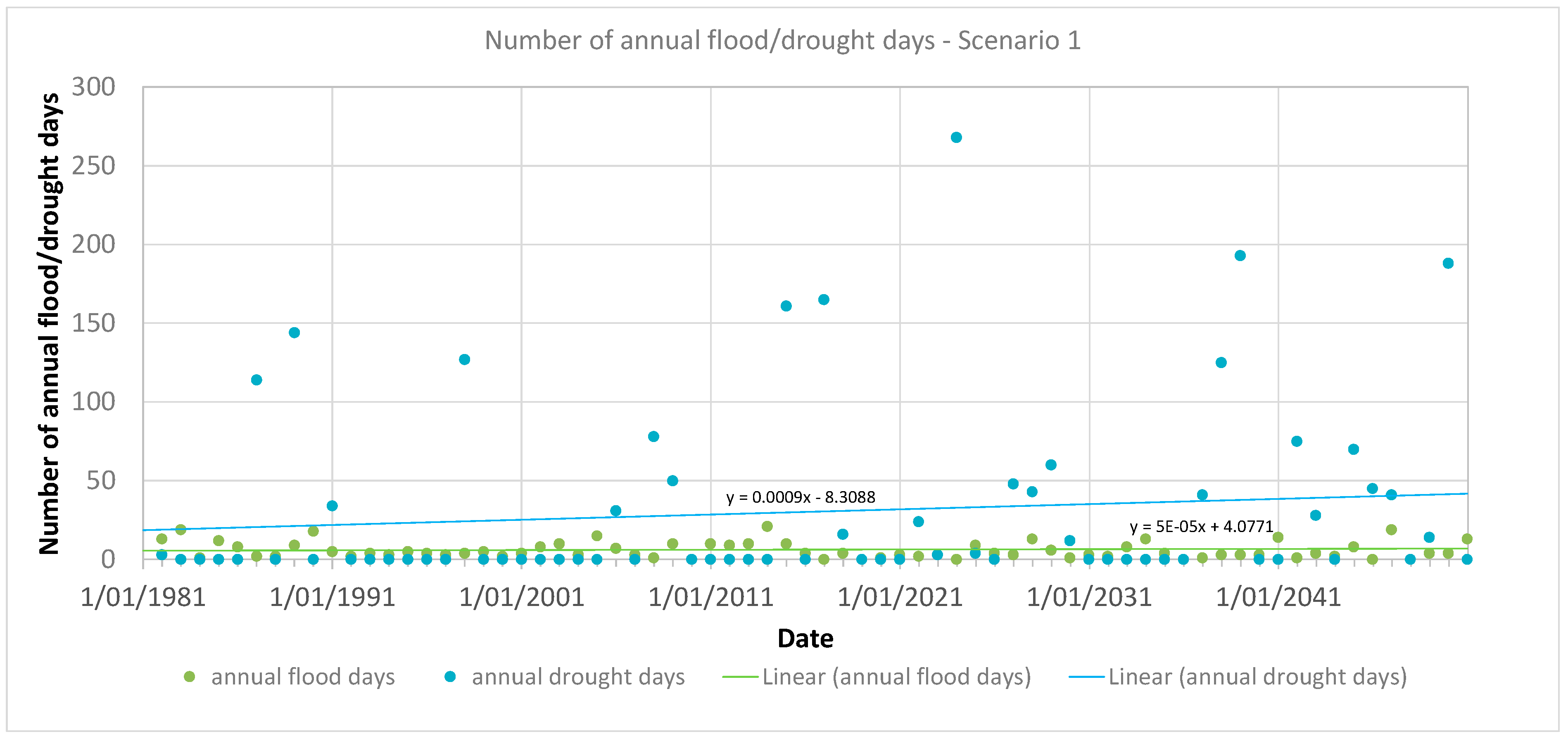
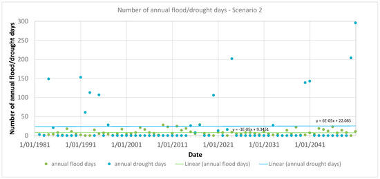
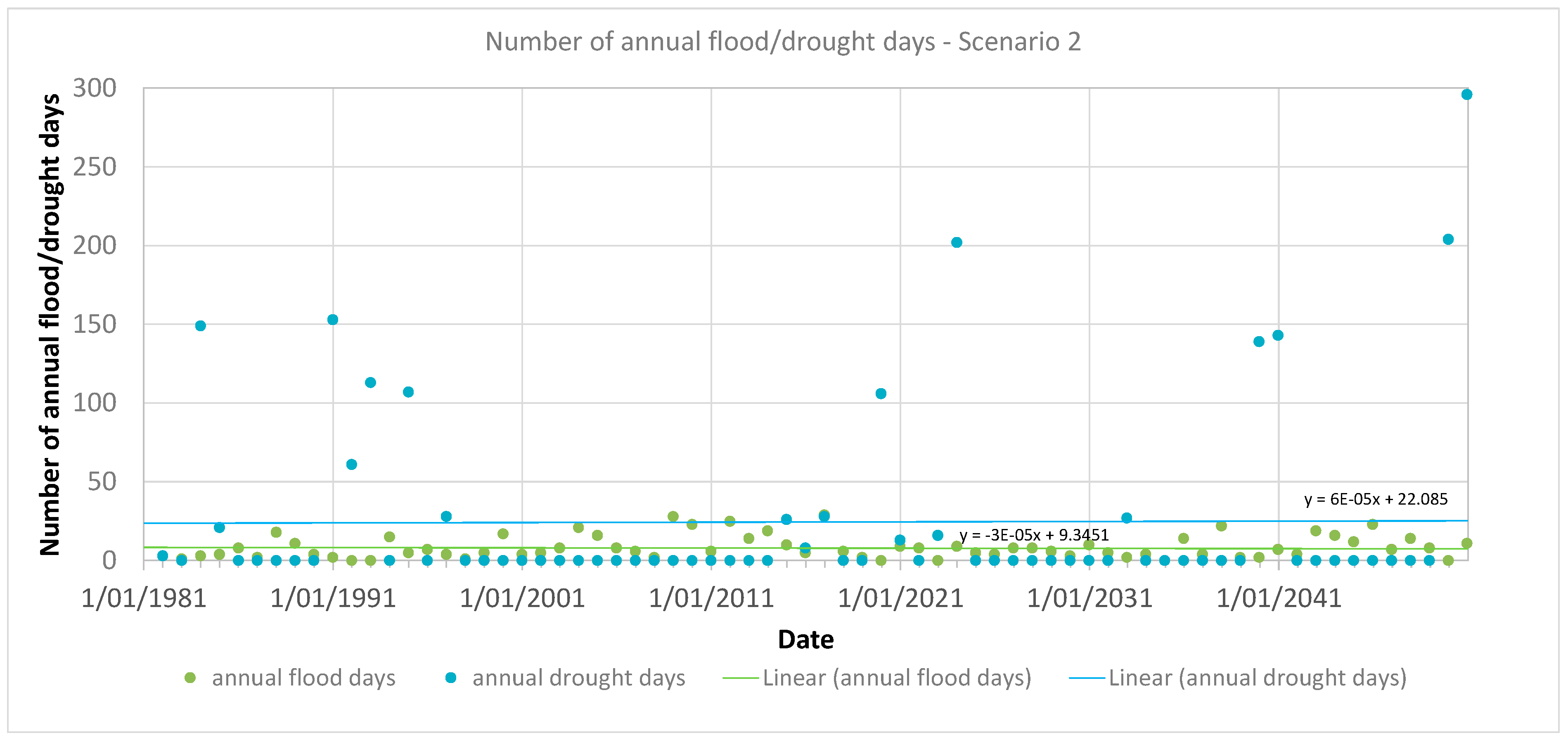
To evaluate how spring discharge evolves over time during the prediction period, the annual counts of flood and drought days were calculated and visualized. Flood days were defined as those with discharge exceeding 0.5 m³/s, while drought days corresponded to discharge falling below 0.1 m³/s. The annual frequencies of flood and drought days under Scenario 1 are displayed in Figure 28, and the corresponding results for Scenario 2 are shown in Figure 29. In Scenario 1 (Figure 28), the number of annual flood days ranges from 0 to 19 throughout the simulation period (1981–2100). A linear regression fitted to the data indicates a slight upward trend. The interannual variability in flood days is relatively limited compared to that of drought days. In contrast, drought conditions in Scenario 1 show a broader range, with annual drought days varying between 0 and 268. The linear regression shows a clear increasing trend in the number of drought days over time. Notably, while most years exhibit few or no flood or drought days, extreme years can feature over 150 drought days. These extreme years appear to follow a periodic pattern, with a recurrence interval of approximately 6 to 9 years. This periodicity becomes more pronounced and severe toward the latter part of the simulation period.

Figure 28. Forecast annual flood and drought days for predictive Scenario 1.

Figure 29. Forecast annual flood and drought days for predictive Scenario 2.

Under Scenario 2 (Figure 29), the annual count of flood days varies from 3 to 28 per year. However, unlike Scenario 1, the linear regression shows a slight decreasing trend over the century. Again, the variability in flood days is relatively minor compared to the more volatile drought day patterns. Drought conditions under Scenario 2 range from 0 to 296 days annually, with the linear trend indicating an increase over time. As in Scenario 1, while most years have zero drought days, extreme years can exceed 150 drought days, showing a recurring periodicity every 6 to 9 years. The frequency and severity of these extreme drought years also appear to intensify over the simulation period.

10. Conclusions

The main aim of this study was to forecast spring discharge under future climate scenarios by utilizing projections from regional climate models (RCMs), with the goal of assessing the potential impacts of climate change on the hydrology of karst springs. To achieve this, a combined statistical–analytical modeling framework was developed, primarily based on rainfall data, and applied specifically to the Jósva spring catchment within the Aggtelek Karst region of Hungary. The model was calibrated against observed spring hydrographs, and projections were driven by two RCM scenarios from the EURO-CORDEX ensemble.

Key findings from the integration of scenario model results include:

• Peak discharge is projected to increase during the first half of the 21st century, followed by a decline toward the century’s end in both scenarios.
• Average discharge is expected to remain largely unchanged throughout the simulation period across both scenarios.
• Baseflow discharge is predicted to decline, though the timing differs: Scenario 1 shows a decline during the first half of the century, whereas Scenario 2 projects a decline in the second half.
• The annual number of flood days exhibits limited variability and no significant long-term trend.
• The annual number of drought days shows a clear increasing trend, with substantial interannual variability.
• Both scenarios indicate a recurring pattern of extremely dry years, with an apparent periodicity of 6 to 9 years.
• The severity of drought years increases over time, as shown by the rising number of drought days in such years.

These findings support the broader conclusion that climate change is likely to amplify hydrological extremes, particularly by increasing drought frequency and severity. This trend holds across both moderate- and high-emission scenarios.

The combined statistical–analytical modeling framework developed in this study proved to be effective for simulating the magnitude and temporal distribution of discharge peaks and baseflow recession based on rainfall data. It offers several advantages:

• Low data requirements, making it suitable for remote or data-scarce karst regions.
• Modular structure, allowing individual components (e.g., regression or baseflow models) to be substituted or enhanced for site-specific needs.
• Physically grounded baseflow estimation, complementing the statistical approach to peak discharge.

Moreover, spectral and wavelet analyses yielded valuable insights for practical applications. The detection of recurring discharge periodicities enhances model interpretability and facilitates the refinement of its statistical components. These periodic signals can be leveraged in early-warning systems to identify periods of heightened drought or flood risk, thus providing a valuable tool for proactive water resource management in data-limited karst environments.

Nonetheless, the study has important limitations. The discharge predictions were based on downscaled climate model outputs and thus inherit the uncertainties inherent to regional climate projections. Moreover, the modeling approach focused solely on rainfall–discharge relationships, with other hydrological components—such as evapotranspiration, soil moisture dynamics, and runoff—implicitly included, but not explicitly modeled. Only two scenarios from a single RCM were used, limiting the generalizability of results. A more comprehensive evaluation that incorporates multiple climate models and emission scenarios would offer a stronger and more reliable understanding of potential future spring discharge patterns. The presented method is best applied to smaller catchments with little spatial geological and climatic variations. Significant snow-dominated recharge and anthropogenic influences can bias model results and thus need to be taken into consideration.

While the methodology demonstrates considerable potential for broader application, particularly in karst terrains, further validation with longer-term datasets and across diverse karst systems is recommended. Future work should also explore the sensitivity of the approach to different climatic, geologic, and hydrologic settings to enhance its utility in regional climate impact assessments.

References

- Stevanovic, Z. Karst waters in potable water supply: A global scale overview. Environ. Earth Sci. 2019, 78, 662. [Google Scholar] [CrossRef] [Scilit]
- Ford, D.; Williams, P. Karst Geomorphology and Hydrology; Unwin Hyman Ltd.: London, UK, 1989. [Google Scholar]
- Hengeveld, H.G. A Discussion of Recent Simulations with CGCM. In Climate Change Digest; Environment Canada: Gatineau, QC, Canada, 2000; p. 32. [Google Scholar]
- Mearns, L.O.; Hulme, M.; Carter, T.R.; Leemans, R.; Lal, M.; Whetton, P. Climate scenario development. In Climate Change 2007: The Physical Science Basis. Contribution of Working Group I to the Fourth Assessment Report of the Intergovernmental Panel on Climate Change; Solomon, S., Qin, D., Manning, M., Chen, Z., Marquis, M., Averyt, K.B., Tignor, M., Miller, H.L., Eds.; Cambridge University Press: Cambridge, UK; New York, NY, USA, 2007; pp. 739–768. [Google Scholar]
- Le Treut, H.; Somerville, R.; Cubasch, U.; Ding, Y.; Mauritzen, C.; Mokssit, A.; Peterson, T.; Prather, M. Historical Overview of Climate Change. In Climate Change 2007: The Physical Science Basis Contribution of Working Group I to the Fourth Assessment Report of the Intergovernmental Panel on Climate Change; Solomon, S., Qin, D., Manning, M., Chen, Z., Marquis, M., Averyt, K.B., Tignor, M., Miller, H.L., Eds.; Cambridge University Press: Cambridge, UK; New York, NY, USA, 2007. [Google Scholar]
- Seneviratne, S.I.; Nicholls, N.; Easterling, D.; Goodess, C.M.; Kanae, S.; Kossin, J.; Luo, Y.; Marengo, J.; McInnes, K.; Rahimi, M.; et al. Changes in climate extremes and their impacts on the natural physical environment. In Managing the Risks of Extreme Events and Disasters to Advance Climate Change Adaptation; Field, C.B., Barros, V., Stocker, T.F., Qin, D., Dokken, D.J., Ebi, K.L., Mastrandrea, M.D., Mach, K.J., Plattner, G.-K., Allen, S.K., et al., Eds.; Cambridge University Press: Cambridge, UK; New York, NY, USA, 2012; pp. 109–230. [Google Scholar]
- Lionello, P.; Scarascia, L. The relation between climate change in the Mediterranean region and global warming. Reg. Environ. Change 2018, 18, 1481–1493. [Google Scholar] [CrossRef] [Scilit]
- Hiscock, K.; Sparkles, R.; Hodgson, A. Evaluation of future climate change impacts on Europe groundwater resources. In Climate Change Effects on Groundwater Resources: A Global Synthesis of Findings and Recommendations; Treidel, H., Martin-Bordes, J.L., Gurdak, J., Eds.; CRC: Boca Raton, FL, USA, 2012; pp. 351–366. [Google Scholar]
- Hartmann, A.; Goldscheider, N.; Wagener, T.; Lange, J.; Weiler, M. Karst water resources in a changing world: Review of hydrological modelling approaches. Rev. Geophys. 2014, 52, 218–242. [Google Scholar] [CrossRef] [Scilit]
- Jenkins, G.M.; Watts, D.G. Spectral Analysis and Its Applications; Holden Days: San Francisco, CA, USA, 1968. [Google Scholar]
- Mangin, A. Etude des débits classés d’exutoires karstiques portant sur un cycle hydrologique. Ann. Spéléol. 1971, 28, 21–40. [Google Scholar]
- Mangin, A. Contribution a L’étude Hydrodynamique des Aquifères Karstiques. Ph.D. Thesis, Université de Dijon, Dijon, France, 1975. [Google Scholar]
- Mangin, A. Utilisation des analyses correlatoire et spectrale dans l’approche des systèmes hydrologiques. Comptes Rendus L’académie Sci.-Ser. III 1981, 293, 401–404. [Google Scholar]
- Mangin, A. Pour une meilleure connaissance des systèmes hydrologiques à partir des analyses corrélatoire et spectrale. J. Hydrol. 1984, 67, 25–43. [Google Scholar] [CrossRef] [Scilit]
- Padilla, A.; Pulido-Bosch, A. Study of hydrographs of karstic aquifers by means of correlation and cross-spectral analysis. J. Hydrol. 1995, 168, 73–89. [Google Scholar] [CrossRef] [Scilit]
- Larocque, M.; Mangin, A.; Razack, M.; Banton, O. Characterization of the La Rochefoucauld karst aquifer (Charente, France) using correlation and spectral analysis. Bull. Hydrogéol. Univ. Neuchâtel 1998, 16, 49–57. [Google Scholar]
- Grasso, D.A. Interprétation Des Réponses Hydrauliques et Chimiques des Sources Karstiques. Ph.D. Thesis, Université de Neuchâtel, Neuchâtel, Switzerland, 1998. [Google Scholar]
- Grasso, D.A.; Jeannin, P.-Y. Etude critique des méthodes d’analyse de la réponse globale des systèmes karstiques. Bull. Hydrogéol. Univ. Neuchâtel 1994, 13, 87–113. [Google Scholar]
- Grasso, D.A.; Jeannin, P.-Y. Statistical approach to the impact of climatic variations on karst spring chemical response. Bull. Hydrogéol. Univ. Neuchâtel 1998, 16, 59–74. [Google Scholar]
- Fiorillo, F.; Esposito, L.; Guadagno, F.M. Analyses and forecast of water resources in an ultra-centenarian spring discharge series from Serino (Southern Italy). J. Hydrol. 2007, 336, 125–138. [Google Scholar] [CrossRef] [Scilit]
- Fiorillo, F.; Doglioni, A. The relation between karst spring discharge and rainfall by the cross-correlation analysis. Hydrogeol. J. 2010, 18, 1881–1895. [Google Scholar] [CrossRef] [Scilit]
- Mero, F. Application of the groundwater depletion curves in analysing and forecasting spring discharges influenced by well fields. In Symposium on Surface Waters; IAHS Publication: Berkeley, CA, USA, 1963; Volume 63, pp. 107–117. [Google Scholar]
- Mero, F. An approach to daily hydrometeorological water balance computations for surface and groundwater basins. In Proceedings of the ITC-UNESCO Seminar for Integrated River Basin Development, Delft, The Netherlands, 20–25 October 1969. [Google Scholar]
- Mero, F.; Gilboa, Y. A methodology for the rapid evaluation of groundwater resources, Sao Paulo State, Brazil. Hydrol. Sci. Bull. 1974, 19, 347–358. [Google Scholar] [CrossRef] [Scilit]
- Bezes, C. Contribution a La Modélisation des Systèmes Aquifères Karstiques. Ph.D. Thesis, Université des Sciences et Techniques du Languedoc, Montpellier, France, 1976. [Google Scholar]
- Thiéry, D. Logiciel GARDÉNIA; Version 8.2; Guide d’utilisation; BRGM: Orléans, France, 2014. [Google Scholar]
- Bailly-Comte, V.; Martin, J.B.; Jourde, H.; Screaton, E.J.; Pistre, S.; Langston, A. Water exchange and pressure transfer between conduits and matrix and their influence on hydrodynamics of two karst aquifers with sinking streams. J. Hydrol. 2010, 386, 55–66. [Google Scholar] [CrossRef] [Scilit]
- Boussinesq, J. Recherches théoriques sur l’écoulement des nappes d’eau infiltrées dans le sol et sur le débit des sources. J. Math. Pures Appl. 1904, 10, 5–78. [Google Scholar]
- Berkaloff, E. Limite de validité des formules courantes de tarissement de débit. Chron. d’Hydrogeol. 1976, 10, 31–41. [Google Scholar]
- Kovács, A. Geometry and Hydraulic Parameters of Karst Aquifers: A Hydrodynamic Modelling Approach. Ph.D. Thesis, University of Neuchatel, Neuchatel, Switzerland, 2003. [Google Scholar]
- Kovács, A.; Perrochet, P.; Király, L.; Jeannin, P.-Y. A quantitative method for the characterization of karst aquifers based on spring hydrograph analysis. J. Hydrol. 2005, 303, 152–164. [Google Scholar] [CrossRef] [Scilit]
- Hornik, K.; Stinchcombe, M.; White, H. Multilayer feedforward networks are universal approximator. Neural Netw. 1989, 2, 359–366. [Google Scholar] [CrossRef] [Scilit]
- Maier, H.R.; Dandy, G.C. Neural networks for the prediction and forecasting of water resources variables: A review of modelling issues and applications. Environ. Model. Softw. 2000, 15, 101–124. [Google Scholar] [CrossRef] [Scilit]
- Corzo, G.; Solomatine, D. Knowledge-based modularization and global optimization of artificial neural network models in hydrological forecasting. Neural Netw. 2007, 20, 528–536. [Google Scholar] [CrossRef] [Scilit] [PubMed]
- Filho, A.J.; dos Santos, C.C. Modelling a densely urbanized watershed with an artificial neural network, weather radar and telemetric data. J. Hydrol. 2006, 317, 34–48. [Google Scholar] [CrossRef] [Scilit]
- Toukourou, M.; Johannet, A.; Dreyfus, G.; Ayral, P.-A. Rainfall-runoff modelling of flash floods in the absence of rainfall forecasts: The case of “Cévenol flash floods”. Appl. Intell. 2011, 35, 178–189. [Google Scholar] [CrossRef] [Scilit]
- Artigue, G.; Johannet, A.; Borrell, V.; Pistre, S. Flash flood forecasting in poorly gauged basins using neural networks: Case study of the Gardon de Mialet basin (southern France). Nat. Hazards Earth Syst. Sci. 2012, 12, 3307–3324. [Google Scholar] [CrossRef] [Scilit]
- Kong-A-Siou, L.; Johannet, A.; Borrell, V.; Pistre, S. Complexity selection of a neural network model for karst flood forecasting: The case of the Lez basin (southern France). J. Hydrol. 2011, 403, 367–380. [Google Scholar] [CrossRef] [Scilit]
- Kurtulus, B.; Razack, M. Evaluation of the ability of an artificial neural network model to simulate the input-output responses of a large karstic aquifer: The La Rochefoucauld aquifer (Charente, France). Hydrogeol. J. 2007, 15, 241–254. [Google Scholar] [CrossRef] [Scilit]
- Kong-A-Siou, L.; Cros, K.; Johannet, A.; Borrell-Estupina, V.; Pistre, S. KnoX method or Knowledge eXtraction from neural network model. Case study on the Lez karst Aquifer (southern France). J. Hydrol. 2013, 507, 19–32. [Google Scholar] [CrossRef] [Scilit]
- Dubois, E.; Doummar, J.; Pistre, S.; Larocque, M. Calibration of a lumped karst system model and application to the Qachqouch karst spring (Lebanon) under climate change conditions. Hydrol. Earth Syst. Sci. 2020, 24, 4275–4290. [Google Scholar] [CrossRef] [Scilit]
- Maillet, E. Essais d’Hydraulique Souterraine et Fluviale; Hermann: Paris, France, 1905. [Google Scholar]
- Forkasiewicz, J.; Paloc, H. Le régime de tarissement de la Foux-de-la-Vis. Etude préliminaire. Chron. d’Hydrogeol. 1967, 3, 61–73. [Google Scholar]
- Schoeller. Hydrodynamique dans le karst, Hydrologie des roches fissurées. In Coedition IAHS/UNESCO; Springer: Dubrovnik, Croatia, 1965. [Google Scholar]
- Kovács, A.; Perrochet, P. A quantitative approach to spring hydrograph decomposition. J. Hydrol. 2008, 352, 16–29. [Google Scholar] [CrossRef] [Scilit]
- Kovács, A.; Perrochet, P. Well hydrograph analysis for the estimation of hydraulic and geometric parameters of karst and connected water systems. In H2Karst Research in Limestone Hydrogeology; Springer International Publishing: Cham, Switzerland, 2014; pp. 97–114. ISBN 978-3-319-06138-2. [Google Scholar]
- Kovács, A.; Perrochet, P.; Darabos, E.; Lénárt, L.; Szűcs, P. Well hydrograph analysis for the characterisation of flow dynamics and conduit network geometry in a karstic aquifer, Bükk Mountains, Hungary. J. Hydrol. 2015, 530, 484–499. [Google Scholar] [CrossRef] [Scilit]
- Kovacs, A. Quantitative classification of carbonate aquifers based on hydrodynamic behaviour. Hydrogeol. J. 2021, 29, 33–52. [Google Scholar] [CrossRef] [Scilit]
- Kovács, A.; Stevanovic, Z. A Combined Statistical–Analytical Method for the Assessment of Climate Change Impact on Spring Discharge. Water 2023, 15, 629. [Google Scholar] [CrossRef] [Scilit]
- Meinshausen, M.; Smith, S.J.; Calvin, K.; Daniel, J.S.; Kainuma, M.; Lamarque, J.; Matsumoto, K.; Montzka, S.; Raper, S.; Riahi, K.; et al. The RCP greenhouse gas concentrations and their extensions from 1765 to 2300. Clim. Change 2011, 109, 213–241. [Google Scholar] [CrossRef] [Scilit]
- Jacob, D.; Petersen, J.; Eggert, B.; Alias, A.; Christensen, O.B.; Bouwer, L.; Braun, A.; Colette, A.; Déqué, M.; Georgievski, G.; et al. EURO-CORDEX: New high-resolution climate change projections for European impact research. Reg. Environ. Change 2013, 14, 563–578. [Google Scholar] [CrossRef] [Scilit]
- IPCC. Climate Change 2013. In The Physical Science Basis. Contribution of Working Group I to the Fifth Assessment Report of the Intergovernmental Panel on Climate Change; Stocker, T.F., Qin, D., Plattner, G.-K., Tignor, M., Allen, S.K., Boschung, J., Nauels, A., Xia, Y., Bex, V., Midgley, P.M., Eds.; Cambridge University Press: Cambridge, UK; New York, NY, USA, 2013; 1535p. [Google Scholar] [CrossRef] [Scilit]
- Szabó, P.; Zsebeházi, G. Report on the Bias Correction of the Ensemble System Containing 10 km Resolution Climate Projections; Third Report of the GINOP-2.3.2-15-2016-00028 Project; HungaroMet Hungarian Meteorological Service: Budapest, Hungary, 2019; 24p. (In Hungarian) [Google Scholar]
- Gruber, P.; Szunyogh, G.; Telbisz, T. The Caves of Aggtelek Karst, Szalonna Karst and Rudabánya Mountains. In Cave and Karst Systems of Hungary; Veress, M., Leél-Őssy, S., Eds.; Springer Nature: Cham, Switzerland, 2022; ISBN 2364-4591. [Google Scholar]
- Less, G.; Grill, J.; Szentpétery, I.; Róth, L.; Gyuricza, G. Geological Map of the Aggtelek-Rudabánya Mountains. In 1:25,000 Scale Uncovered Geological Map; Geological Institute of Hungary: Budapest, Hungary, 1988. [Google Scholar]
- Telbisz, T.; Mari, L.; Gruber, P.; Kőszegi, M. Geological heritage, Geoturism and Local Development in Aggtelek National Park (NW Hungary). Geoheritage 2020, 12, 5. [Google Scholar] [CrossRef] [Scilit]
- Gregor, M.; Malík, P. Construction of Master Recession Curve Using Genetic Algorithms. J. Hydrol. Hydromech. 2012, 60, 3–15. [Google Scholar] [CrossRef] [Scilit]
- Ilyés, C.; Turai, E.; Szűcs, P.; Zsuga, J. Examination of the cyclic properties of 110-year-long precipitation time series. Acta Montan. Slovaca 2017, 22, 1–11. [Google Scholar]
- Ilyés, C.; Turai, E.; Szűcs, P. Examination of rainfall data for 110 years using spectral and wavelet analysis. Cent. Eur. Geol. 2018, 61, 1–15. [Google Scholar] [CrossRef] [Scilit]
- Garamhegyi, T.; Kovács, J.; Pongrácz, R.; Tanos, P.; Hatvani, I.G. Investigation of the climate-driven periodicity of shallow groundwater level fluctuations in a Central-Eastern European agricultural region. Hydrogeol. J. 2018, 26, 677–688. [Google Scholar] [CrossRef] [Scilit]
Disclaimer/Publisher’s Note: The statements, opinions and data contained in all publications are solely those of the individual author(s) and contributor(s) and not of MDPI and/or the editor(s). MDPI and/or the editor(s) disclaim responsibility for any injury to people or property resulting from any ideas, methods, instructions or products referred to in the content. |
© 2025 by the authors. Licensee MDPI, Basel, Switzerland. This article is an open access article distributed under the terms and conditions of the Creative Commons Attribution (CC BY) license (https://creativecommons.org/licenses/by/4.0/).