
Dynamic Response Characteristics of Shallow Groundwater Level to Hydro-Meteorological Factors and Well Irrigation Water Withdrawals under Different Conditions of Groundwater Buried Depth
Abstract
:1. Introduction
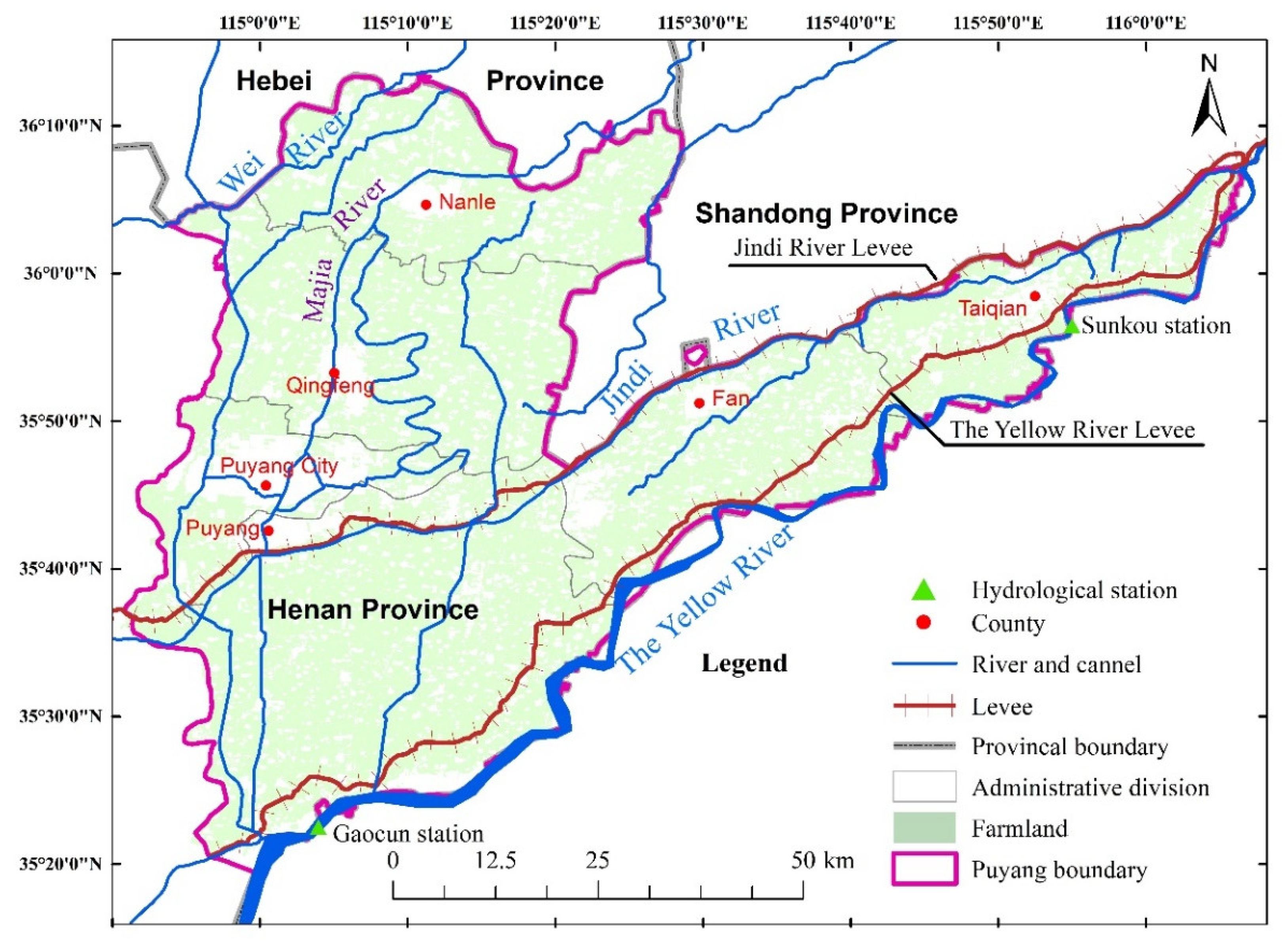
2. Study Area
3. Data and Methodology
3.1. Data Collection
3.2. Estimation of Groundwater Pumpage for Irrigation
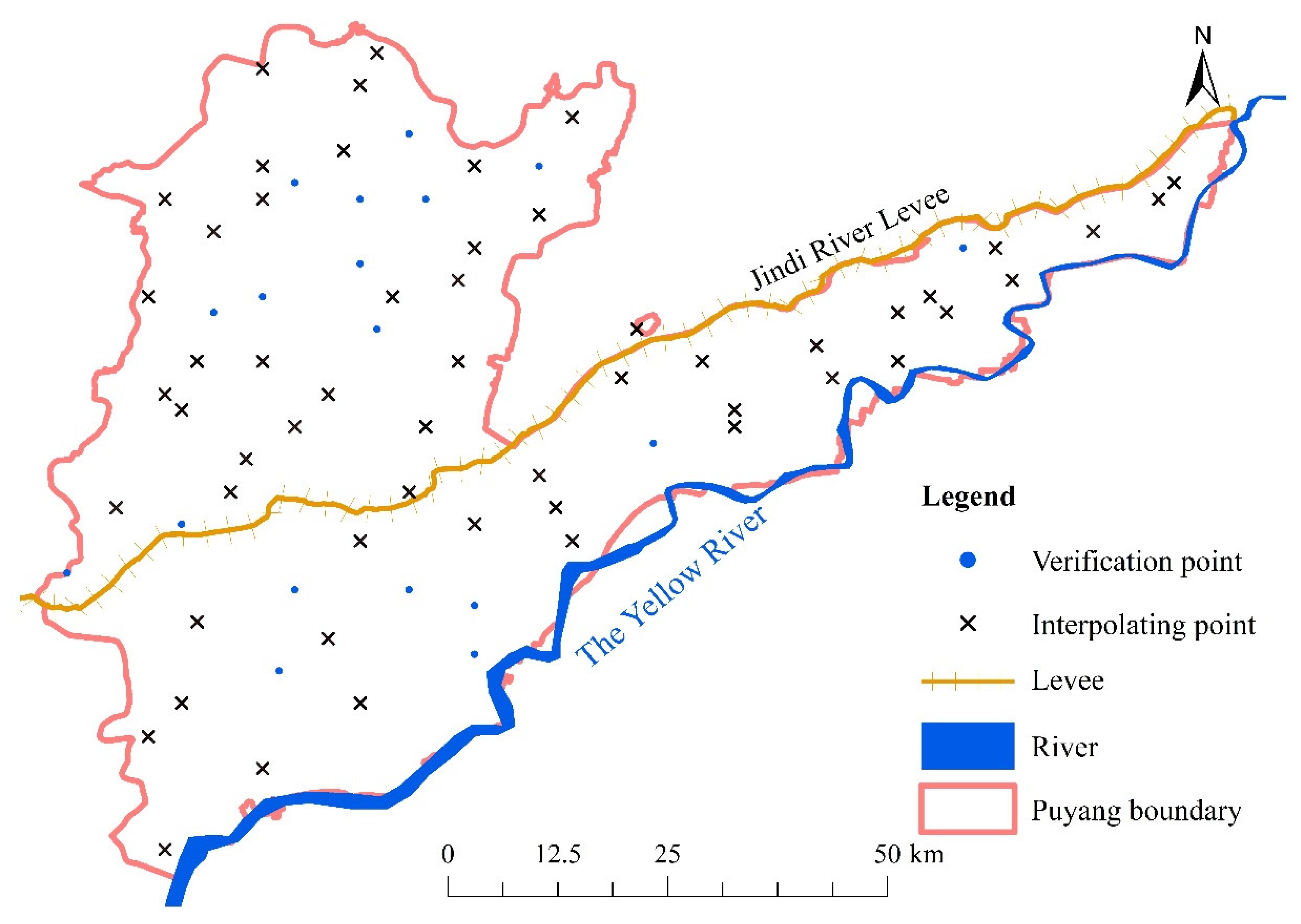
3.3. Spatial Interpolation of Groundwater Depth
3.4. Wavelet Analysis
4. Results and Discussion
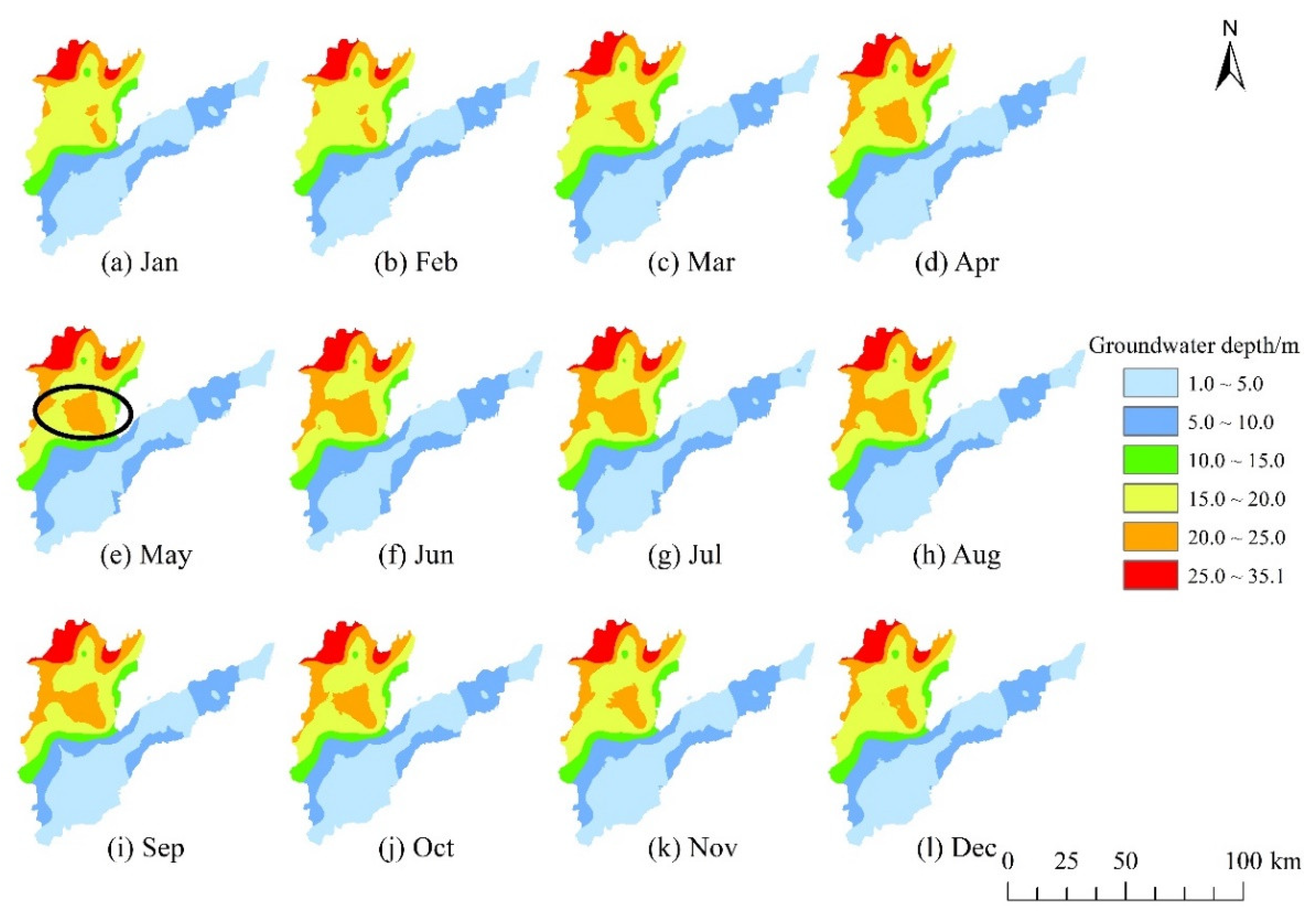
4.1. Spatio-Temporal Variation of Buried Depth of Shallow Groundwater
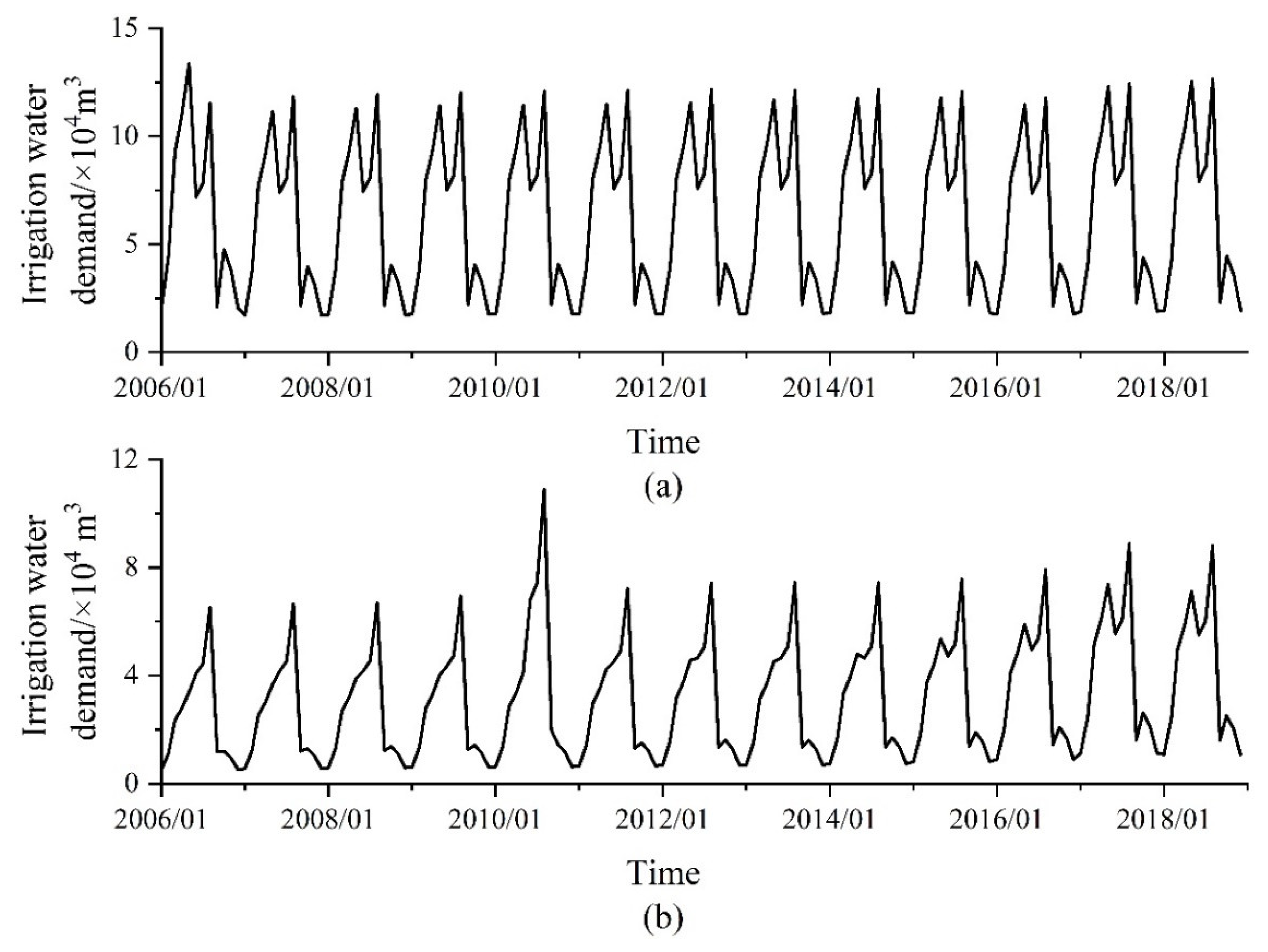
4.2. Variation of Well Irrigation Water Amount
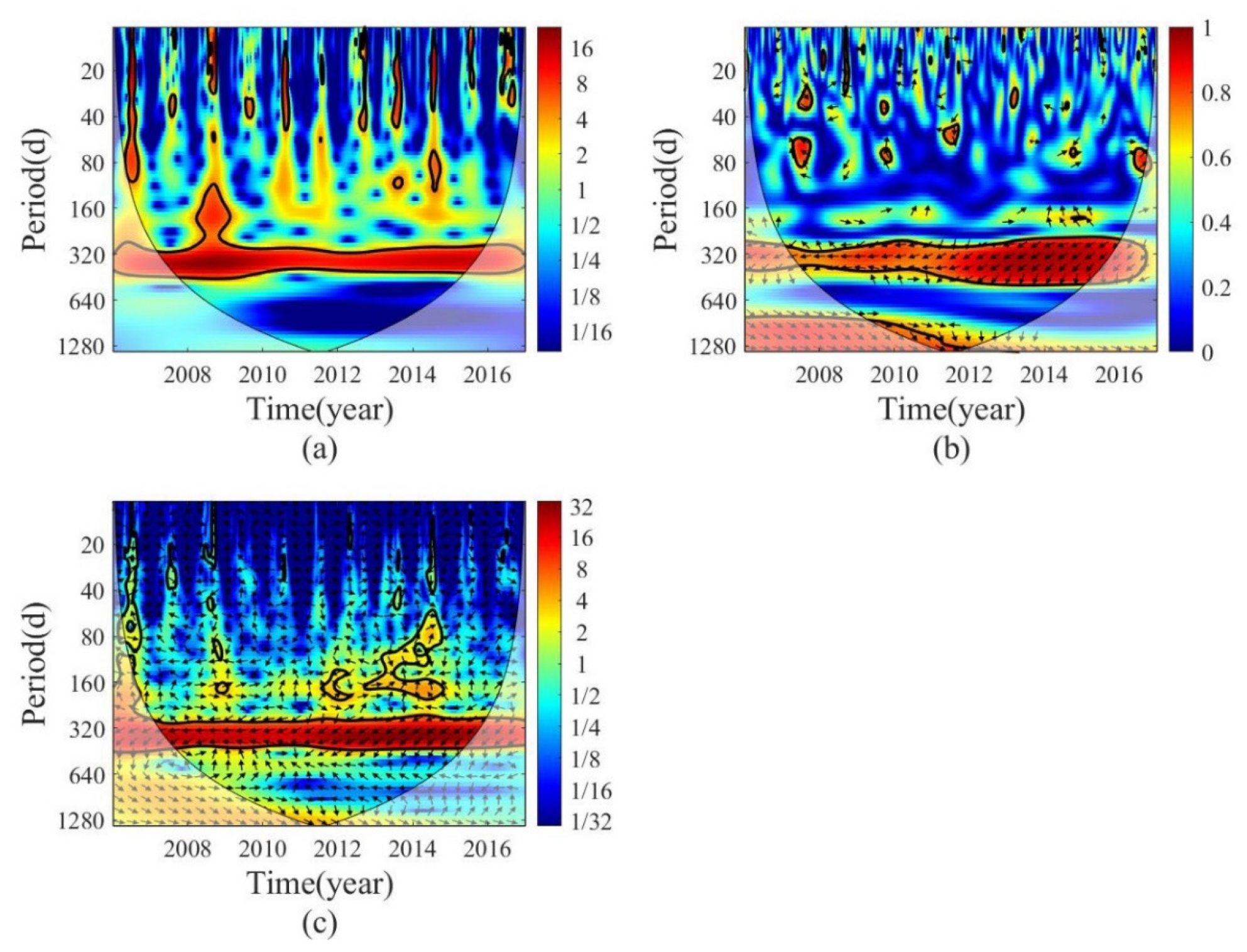
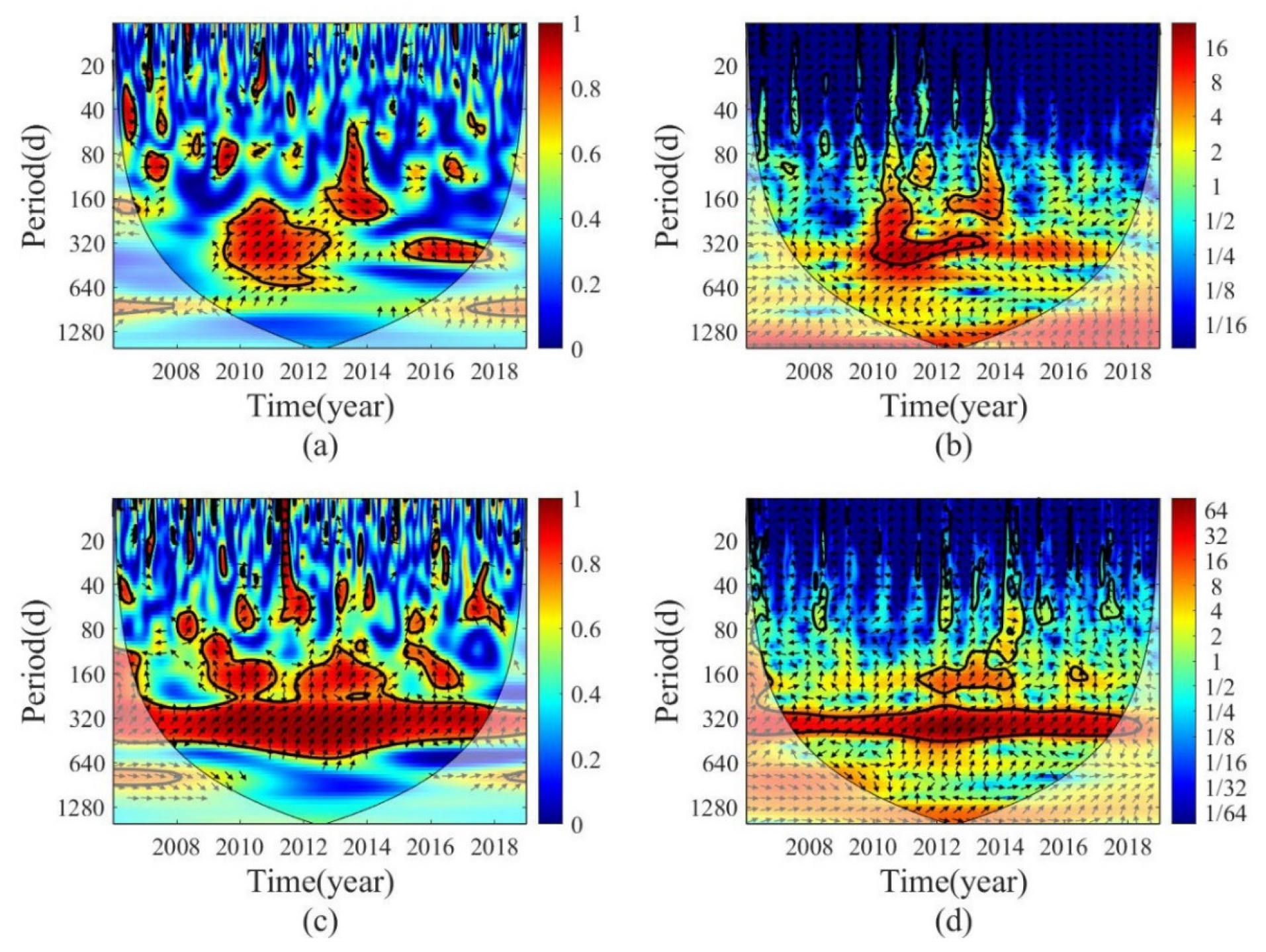
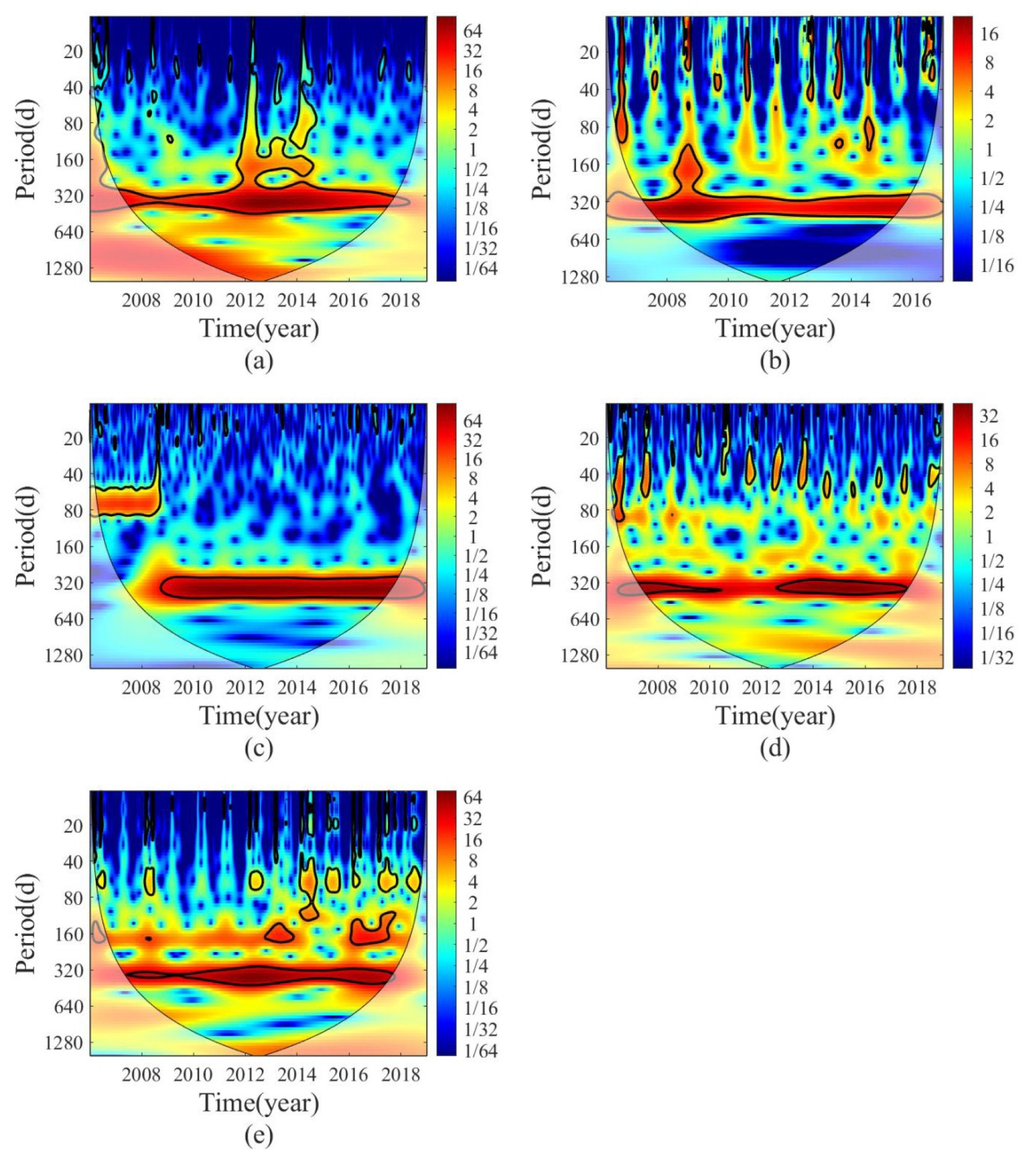
4.3. Cross Wavelet Coherence Analysis of Groundwater Level and Different Factors
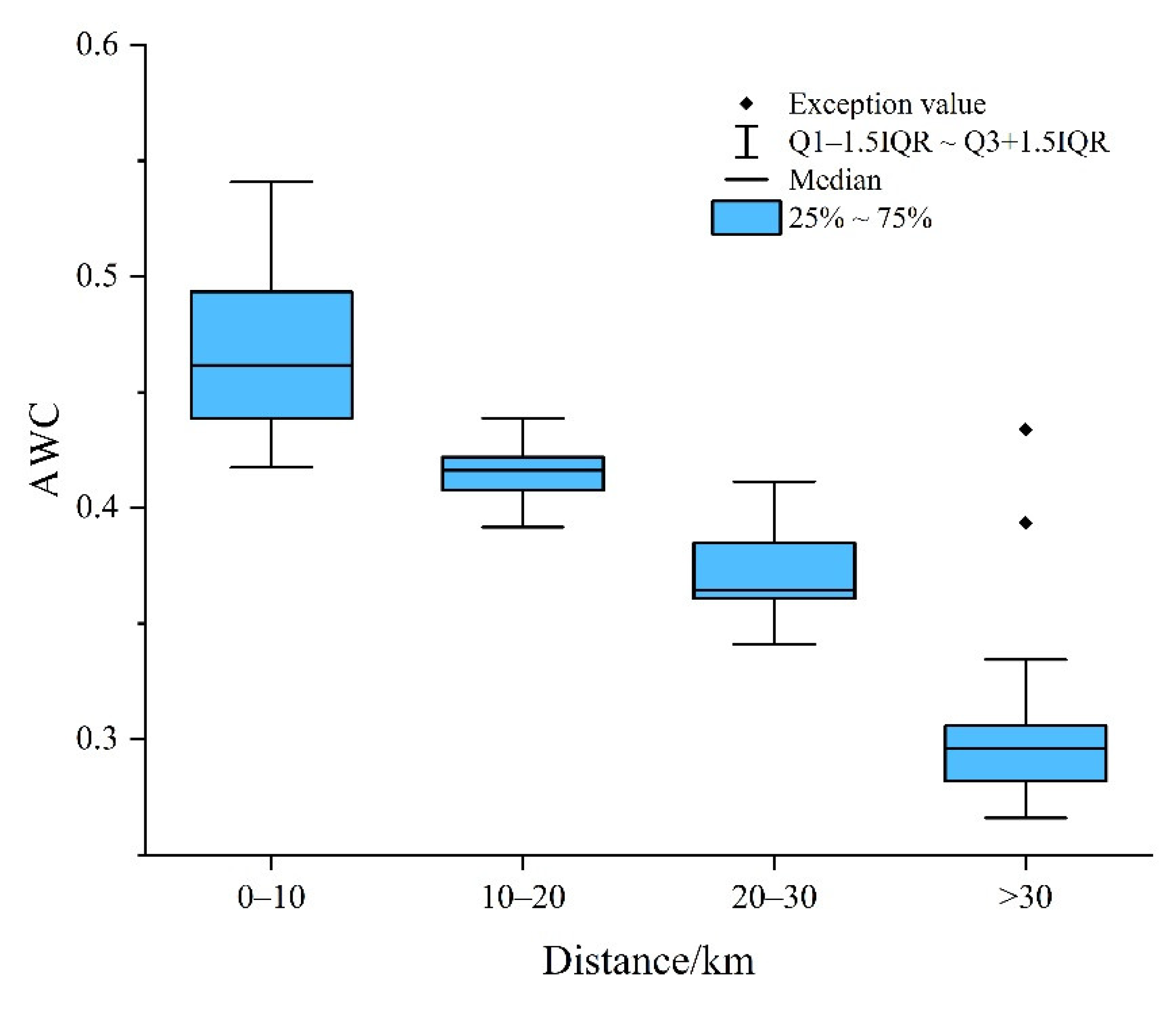
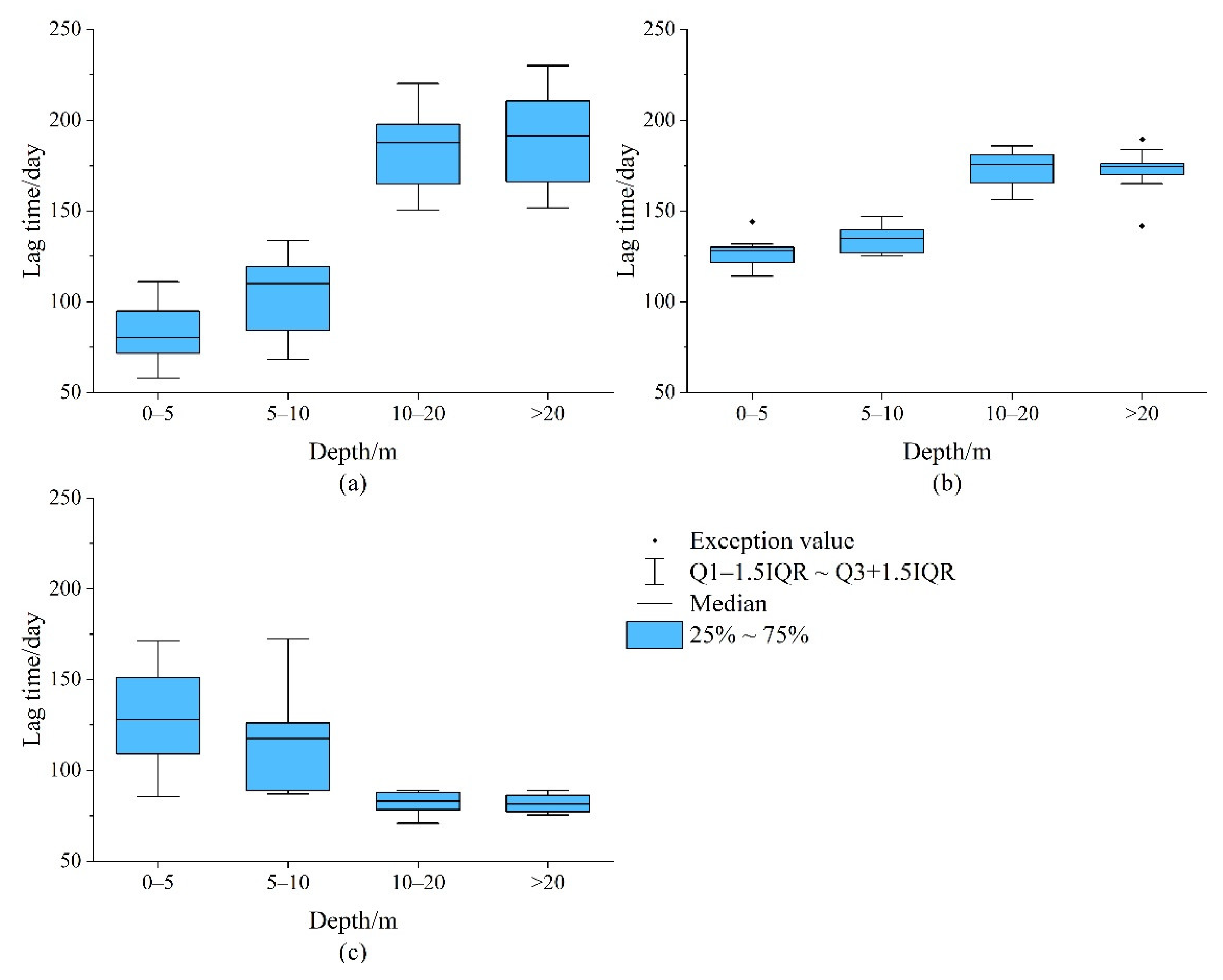
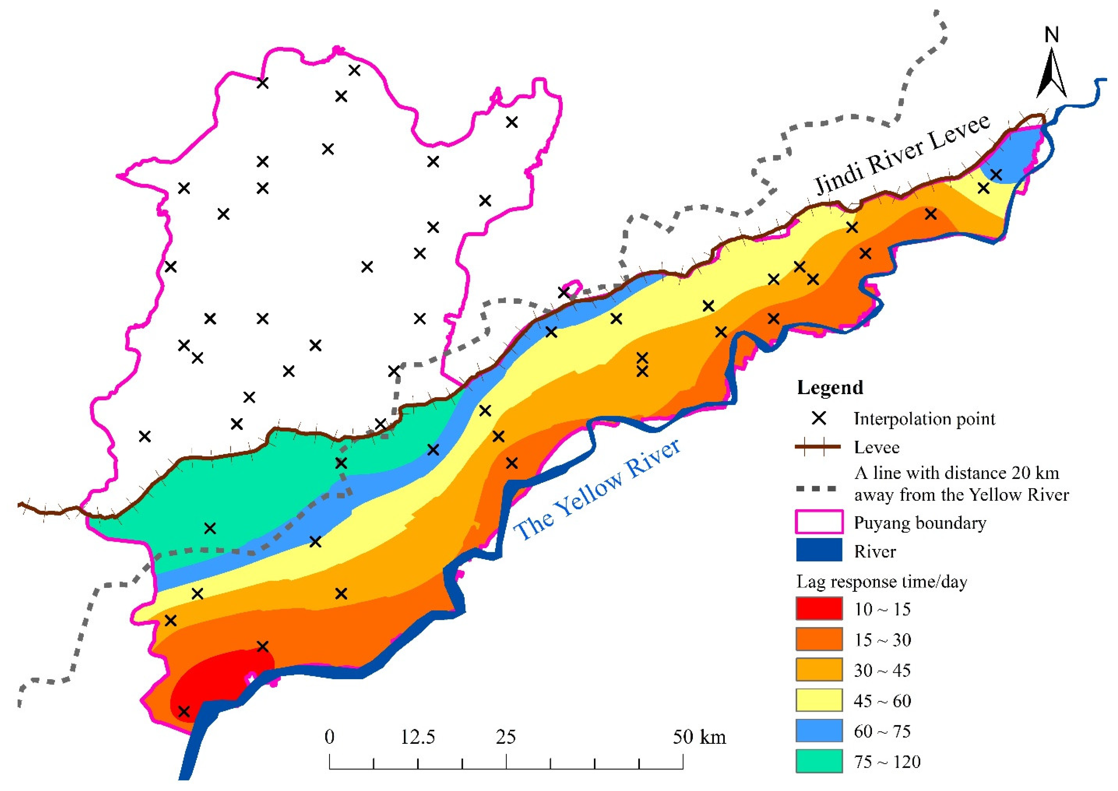
4.4. Response Time of Groundwater Level to Influencing Factors
5. Conclusions
Author Contributions
Funding
Institutional Review Board Statement
Informed Consent Statement
Data Availability Statement
Acknowledgments
Conflicts of Interest
References
- Döll, P.; Hoffmann-Dobrev, H.; Portmann, F.T.; Siebert, S.; Eicker, A.; Rodell, M.; Strassberg, G.; Scanlon, B.R. Impact of water withdrawals from groundwater and surface water on continental water storage variations. J. Geodyn. 2012, 59–60, 143–156. [Google Scholar] [CrossRef]
- Roy, D.K.; Biswas, S.K.; Saha, K.K.; Ibn Murad, K.F. Groundwater level forecast via a discrete space-state modelling approach as a surrogate to complex groundwater simulation modelling. Water Resour. Manag. 2021, 35, 1653–1672. [Google Scholar] [CrossRef]
- Castellazzi, P.; Martel, R.; Galloway, D.L.; Longuevergne, L.; Rivera, A. Assessing groundwater depletion and dynamics using GRACE and InSAR: Potential and limitations. Groundwater 2016, 54, 768–780. [Google Scholar] [CrossRef] [Green Version]
- Celik, R. Temporal changes in the groundwater level in the Upper Tigris Basin, Turkey, determined by a GIS technique. J. Afr. Earth Sci. 2015, 107, 134–143. [Google Scholar] [CrossRef]
- Ojha, C.; Werth, S.; Shirzaei, M. Recovery of aquifer-systems in Southwest US following 2012–2015 drought: Evidence from InSAR, GRACE and groundwater level data. J. Hydrol. 2020, 587, 124943. [Google Scholar] [CrossRef]
- Rodell, M.; Famiglietti, J.S.; Wiese, D.N.; Reager, J.T.; Beaudoing, H.K.; Landerer, F.W.; Lo, M.-H. Emerging trends in global freshwater availability. Nature 2018, 557, 651–659. [Google Scholar] [CrossRef]
- Gu, X.; Sun, H.; Zhang, Y.; Zhang, S.; Lu, C. Partial wavelet coherence to evaluate scale-dependent relationships between precipitation/surface water and groundwater levels in a groundwater system. Water Resour. Manag. 2022, 36, 2509–2522. [Google Scholar] [CrossRef]
- Narany, T.S.; Aris, A.Z.; Sefie, A.; Keesstra, S. Detecting and predicting the impact of land use changes on groundwater quality, a case study in Northern Kelantan, Malaysia. Sci. Total Environ. 2017, 599–600, 844–853. [Google Scholar] [CrossRef]
- Qu, J.; Zhang, Y.; Zou, X. Evaluation of groundwater function in Puyang City based on dissipation theory. Water Resour. Hydropower Eng. 2019, 50, 70–77. (In Chinese) [Google Scholar] [CrossRef]
- Ali, M.Z.; Chu, H.; Burbey, T.J. Mapping and predicting subsidence from spatio-temporal regression models of groundwater-drawdown and subsidence observations. Hydrogeol. J. 2020, 28, 2865–2876. [Google Scholar] [CrossRef]
- Sarma, R.; Singh, S.K. A comparative study of data-driven models for groundwater level forecasting. Water Resour. Manag. 2022, 36, 2741–2756. [Google Scholar] [CrossRef]
- Xu, M.; Kang, S.; Chen, X.; Wu, H.; Wang, X.; Su, Z. Detection of hydrological variations and their impacts on vegetation from multiple satellite observations in the Three-River Source Region of the Tibetan Plateau. Sci. Total Environ. 2018, 639, 1220–1232. [Google Scholar] [CrossRef]
- Dench, W.E.; Morgan, L.K. Unintended consequences to groundwater from improved irrigation efficiency: Lessons from the Hinds-Rangitata Plain, New Zealand. Agric. Water Manage. 2021, 245, 106530. [Google Scholar] [CrossRef]
- Dey, S.; Dey, A.K.; Mall, R.K. Modeling long-term groundwater levels by exploring deep bidirectional Long Short-Term Memory using hydro-climatic data. Water Resour. Manag. 2021, 35, 3395–3410. [Google Scholar] [CrossRef]
- Lin, M.; Biswas, A.; Bennett, E.M. Identifying hotspots and representative monitoring area of groundwater changes with time stability analysis. Sci. Total Environ. 2019, 667, 419–426. [Google Scholar] [CrossRef]
- Zhao, Z.; Jia, Z.; Guan, Z.; Xu, C. The Effect of climatic and non-climatic factors on groundwater levels in the Jinghuiqu irrigation district of the Shaanxi Province, China. Water 2019, 11, 956. [Google Scholar] [CrossRef] [Green Version]
- Leblanc, M.J.; Tregoning, P.; Ramillien, G.; Tweed, S.O.; Fakes, A. Basin-scale, integrated observations of the early 21st century multiyear drought in southeast Australia. Water Resour. Res. 2009, 45, W04408. [Google Scholar] [CrossRef] [Green Version]
- Bahita, T.A.; Swain, S.; Dayal, D.; Jha, P.K.; Pandey, A. Water quality assessment of Upper Ganga Canal for human drinking. In Climate Impacts on Water Resources in India, 1st ed.; Pandey, A., Mishra, S.K., Kansal, M.L., Singh, R.D., Singh, V.P., Eds.; Springer: Cham, Switzerland, 2021; pp. 371–392. [Google Scholar] [CrossRef]
- Xiao, Y.; Gu, X.; Yin, S.; Shao, J.; Cui, Y.; Zhang, Q.; Niu, Y. Geostatistical interpolation model selection based on ArcGIS and spatio-temporal variability analysis of groundwater level in piedmont plains, northwest China. SpringerPlus 2016, 5, 425. [Google Scholar] [CrossRef] [Green Version]
- Shih, D.C.F. Storage in confined aquifer: Spectral analysis of groundwater in responses to Earth tides and barometric effect. Hydrol. Process. 2018, 32, 1927–1935. [Google Scholar] [CrossRef]
- Liu, Q.; Chen, S.; Jiang, L.; Wang, D.; Yang, Z.; Chen, L. Determining thermal diffusivity using near-surface periodic temperature variations and its implications for tracing groundwater movement at the eastern margin of the Tibetan Plateau. Hydrol. Process. 2019, 33, 1276–1286. [Google Scholar] [CrossRef]
- Cheng, Y.; Lin, M.; Wu, J.; Zhu, H.; Shao, X. Intelligent fault diagnosis of rotating machinery based on continuous wavelet transform-local binary convolutional neural network. Knowl. Based Syst. 2021, 216, 106796. [Google Scholar] [CrossRef]
- Li, J.; Pu, J.; Zhang, T.; Wang, S.; Huo, W.; Yuan, D. Investigation of transport properties and characteristics of a large karst aquifer system in southern China using correlation, spectral, and wavelet analyses. Environ. Earth Sci. 2021, 80, 84. [Google Scholar] [CrossRef]
- Zhang, M.; Wang, Y.; Wang, X.; Zhou, W. Groundwater depth forecasting using a coupled model. Discrete Dyn. Nat. Soc. 2021, 2021, 6614195. [Google Scholar] [CrossRef]
- Cao, R.; Jiang, R.; Zhao, Y.; Xie, J.; Yu, X. Spatiotemporal characteristics of groundwater depth in Xingtai city on the North China Plain: Changing patterns, causes and prediction. Appl. Ecol. Environ. Res. 2020, 18, 6605–6622. [Google Scholar] [CrossRef]
- Ling, M.; Han, H.; Wei, X.; Lv, C. Temporal and spatial distributions of precipitation on the Huang-Huai-Hai Plain during 1960-2019, China. J. Water Clim. Chang. 2021, 12, 2232–2244. [Google Scholar] [CrossRef]
- Gordu, F.; Nachabe, M.H. A physically constrained wavelet-aided statistical model for multi-decadal groundwater dynamics predictions. Hydrol. Process. 2021, 35, e14308. [Google Scholar] [CrossRef]
- Wu, C.; Zhang, X.; Wang, W.; Lu, C.; Zhang, Y.; Qin, W.; Tick, G.R.; Liu, B.; Shu, L. Groundwater level modeling framework by combining the wavelet transform with a long short-term memory data-driven model. Sci. Total Environ. 2021, 783, 146948. [Google Scholar] [CrossRef]
- Cui, Y.; Liao, Z.; Wei, Y.; Xu, X.; Song, Y.; Liu, H. The response of groundwater level to climate change and human activities in Baotou City, China. Water 2020, 12, 1078. [Google Scholar] [CrossRef]
- Clyne, J.B.; Sawyer, A.H. Groundwater-stream connectivity from minutes to months across United States basins as revealed by spectral analysis. Hydrol. Process. 2022, 36, e14514. [Google Scholar] [CrossRef]
- Qi, H. Responsive change in groundwater table in karst to precipitation and Yellow River in Pingyin County. J. Irrig. Drain. 2019, 38, 94–100. (In Chinese) [Google Scholar] [CrossRef]
- Dong, L.; Guo, Y.; Tang, W.; Xu, W.; Fan, Z. Statistical evaluation of the influences of precipitation and river level fluctuations on groundwater in Yoshino River Basin, Japan. Water 2022, 14, 625. [Google Scholar] [CrossRef]
- Yang, T.; Ala, M.; Guan, D.; Wang, A. The effects of groundwater depth on the soil evaporation in Horqin Sandy Land, China. Chin. Geogr. Sci. 2021, 31, 727–734. [Google Scholar] [CrossRef]
- PWCB. Puyang Water Resources Bulletin in 2018; Puyang Water Conservancy Bureau: Puyang, China, 2019; pp. 6–8. (In Chinese) [Google Scholar]
- Cai, Y.; Mitani, Y.; Ikemi, H.; Liu, S. Effect of precipitation timescale selection on tempo-spatial assessment of paddy water demand in Chikugo-Saga Plain, Japan. Water Resour. Manag. 2012, 26, 1731–1746. [Google Scholar] [CrossRef]
- Feng, F.; Jiang, N.; Feng, Y.; Wang, M.; Gao, Z.; Zhang, Z. Water requirement calculation and trend analysis of main crops in Yellow River irrigation area. Yellow River 2021, 43, 165–170. (In Chinese) [Google Scholar] [CrossRef]
- Liang, W. Study on Measuring Crop Evapotranspiration and Crop Coefficients Changes for Winter Wheat and Maize. Master’s Thesis, Northwest A&F University, Xianyang, China, 2012. (In Chinese). [Google Scholar]
- Ghosh, A.; Pahari, P.; Basak, P.; Maulik, U.; Sarkar, A. Epileptic-seizure onset detection using PARAFAC model with cross-wavelet transformation on multi-channel EEG. Phys. Eng. Sci. Med. 2022, 45, 601–612. [Google Scholar] [CrossRef]
- Mandler, M.; Scharnagl, M. Financial cycles in euro area economies: A cross-country perspective using wavelet analysis. Oxf. Bull. Econ. Stat. 2022, 84, 569–593. [Google Scholar] [CrossRef]
- Caccamo, M.T.; Cannuli, A.; Magazu, S. Wavelet analysis of near-resonant series RLC circuit with time-dependent forcing frequency. Eur. J. Phys. 2018, 39, 045702. [Google Scholar] [CrossRef]
- Niu, S.; Shu, L.; Li, H.; Xiang, H.; Wang, X.; Opoku, P.A.; Li, Y. Identification of preferential runoff belts in Jinan Spring Basin based on hydrological time-series correlation. Water 2021, 13, 3255. [Google Scholar] [CrossRef]
- Torrence, C.; Webster, P. Interdecadal changes in the ESNO-Monsoon system. J. Clim. 1999, 12, 2679–2690. [Google Scholar] [CrossRef]
- Nalley, D.; Adamowski, J.; Biswas, A.; Gharabaghi, B.; Hu, W. A multiscale and multivariate analysis of precipitation and streamflow variability in relation to ENSO, NAO and PDO. J. Hydrol. 2019, 574, 288–307. [Google Scholar] [CrossRef]
- Wang, J.; Kong, D.; Yin, X.; Xue, B. Quantitative study on bed morphology adjustment of the wandering reaches of the lower Yellow River in recent 70 years. Fresenius Environ. Bull. 2022, 31, 3754–3765. [Google Scholar]
- Grinsted, A.; Moore, J.C.; Jevrejeva, S. Application of the cross wavelet transform and wavelet coherence to geophysical time series. Nonlin. Process. Geophys. 2004, 11, 561–566. [Google Scholar] [CrossRef]
- Malik, M.S.; Shukla, J.P.; Mishra, S. Effect of groundwater level on soil moisture, soil temperature and surface temperature. J. Indian Soc. Remote Sens. 2021, 49, 2143–2161. [Google Scholar] [CrossRef]
- Zhao, Y.; Shao, J.; Yan, Z.; Jiao, H.; Cui, Y.; He, G. A comprehensive approach to groundwater system boundaries along the zone affected by the lower reaches of the Yellow River. Acta Geosci. Sin. 2004, 25, 99–102. (In Chinese) [Google Scholar]
- Cai, Y.; Xu, J.; Zhu, Q.; Rao, Y.; Cao, Y. Spatiotemporal variation of shallow groundwater in Puyang of Henan Province and its underlying determinants. J. Irrig. Drain. 2021, 40, 109–116. (In Chinese) [Google Scholar] [CrossRef]
- Li, X.; Hao, J.; Wang, Y. Discuss on three-type water transformation relations and patterns in the Huanghe River Basin. Arid Land Geogr. 2010, 33, 607–614. (In Chinese) [Google Scholar] [CrossRef]
- Wang, J.; Shi, B.; Zhao, E.; Chen, X.; Yang, S. Synergistic effects of multiple driving factors on the runoff variations in the Yellow River Basin, China. J. Arid Land 2021, 13, 835–857. [Google Scholar] [CrossRef]


| Year | Precipitation/mm | Water Level (AMSL) at Gaocun Station/m | Crop Planting Area/km2 | ||||
|---|---|---|---|---|---|---|---|
| Winter Wheat | Summer Maize | ||||||
| North | South | Average | North | South | North | South | |
| 2006 | 434.9 | 443.8 | 59.57 | 1409.4 | 910.9 | 357.8 | 515.6 |
| 2007 | 491.0 | 576.4 | 59.41 | 1174.6 | 935.7 | 386.7 | 525.6 |
| 2008 | 590.7 | 504.6 | 59.13 | 1193.6 | 943.1 | 410.6 | 527.6 |
| 2009 | 542.1 | 582.9 | 58.80 | 1204.9 | 950.1 | 424.0 | 548.8 |
| 2010 | 721.7 | 703.0 | 58.92 | 1208.6 | 954.6 | 431.1 | 861.6 |
| 2011 | 583.9 | 592.9 | 58.93 | 1213.3 | 958.1 | 448.4 | 570.4 |
| 2012 | 438.3 | 348.5 | 59.04 | 1219.2 | 961.4 | 482.0 | 586.9 |
| 2013 | 447.6 | 443.4 | 58.72 | 1232.0 | 958.4 | 475.9 | 588.1 |
| 2014 | 531.3 | 504.1 | 58.47 | 1241.0 | 961.3 | 505.9 | 588.0 |
| 2015 | 543.2 | 556.8 | 58.38 | 1243.7 | 953.9 | 564.6 | 597.5 |
| 2016 | 560.2 | 541.4 | 56.59 | 1210.7 | 930.4 | 621.4 | 625.4 |
| 2017 | 480.0 | 515.9 | 56.48 | 1298.5 | 983.6 | 778.3 | 701.8 |
| 2018 | 594.5 | 625.2 | 57.13 | 1323.7 | 1000.2 | 750.2 | 696.3 |
| Stage | Kc | ET0/mm | ||
|---|---|---|---|---|
| Winter Wheat | Summer Maize | Winter Wheat | Summer Maize | |
| Seeding stage | 0.70 | 0.62 | 52.24 | 45.87 |
| Stooling stage | 0.69 | - | 44.08 | - |
| Emergence stage | - | 0.68 | - | 78.64 |
| Overwintering stage | 0.51 | - | 81.14 | - |
| Regreening stage | 0.72 | - | 83.28 | - |
| Jointing stage | 0.90 | 0.97 | 85.89 | 86.32 |
| Tasseling stage | - | 1.08 | - | 100.58 |
| Heading stage | 1.08 | - | 79.68 | - |
| Filling stage | 0.62 | 0.68 | 104.23 | 55.65 |
| Maturation stage | - | - | - | - |
| Interpolation Method | MAE/m | MRE/% | RMSE/% |
|---|---|---|---|
| Trend Surface | 1.45 | 3.13 | 3.01 |
| Regular Spline | 1.65 | 3.21 | 2.87 |
| Ordinary Kriging | 0.18 | 0.23 | 0.63 |
| Inverse Distance Weight | 0.71 | 1.34 | 1.58 |
| Simple Kriging | 0.26 | 0.38 | 1.29 |
| Depth/m | Precipitation | Air Temperature | The Yellow River Water Stage | Well Irrigation | ||||
|---|---|---|---|---|---|---|---|---|
| AWC | PASC/% | AWC | PASC/% | AWC | PASC/% | AWC | PASC/% | |
| 0–5 | 0.50 | 32.71 | 0.51 | 26.79 | 0.45 | 29.92 | 0.48 | 30.79 |
| 5–10 | 0.42 | 25.40 | 0.43 | 26.41 | 0.42 | 28.36 | 0.48 | 30.74 |
| 10–20 | 0.35 | 22.74 | 0.34 | 29.13 | 0.30 | 28.73 | 0.47 | 29.98 |
| >20 | 0.25 | 23.06 | 0.32 | 26.81 | 0.34 | 28.29 | 0.51 | 30.52 |
Publisher’s Note: MDPI stays neutral with regard to jurisdictional claims in published maps and institutional affiliations. |
© 2022 by the authors. Licensee MDPI, Basel, Switzerland. This article is an open access article distributed under the terms and conditions of the Creative Commons Attribution (CC BY) license (https://creativecommons.org/licenses/by/4.0/).
Share and Cite
Cai, Y.; Huang, R.; Xu, J.; Xing, J.; Yi, D. Dynamic Response Characteristics of Shallow Groundwater Level to Hydro-Meteorological Factors and Well Irrigation Water Withdrawals under Different Conditions of Groundwater Buried Depth. Water 2022, 14, 3937. https://doi.org/10.3390/w14233937
Cai Y, Huang R, Xu J, Xing J, Yi D. Dynamic Response Characteristics of Shallow Groundwater Level to Hydro-Meteorological Factors and Well Irrigation Water Withdrawals under Different Conditions of Groundwater Buried Depth. Water. 2022; 14(23):3937. https://doi.org/10.3390/w14233937
Chicago/Turabian StyleCai, Yi, Ruoyao Huang, Jia Xu, Jingwen Xing, and Dongze Yi. 2022. "Dynamic Response Characteristics of Shallow Groundwater Level to Hydro-Meteorological Factors and Well Irrigation Water Withdrawals under Different Conditions of Groundwater Buried Depth" Water 14, no. 23: 3937. https://doi.org/10.3390/w14233937