
Physical and Biological Features of the Waters in the Outer Patagonian Shelf and the Malvinas Current
 , , , , , , , , , , add
Show full author list
, , , , , , , , , , add
Show full author list
Abstract
:1. Introduction
2. Materials and Methods
2.1. Field Oceanographic and Optical Measurements
2.1.1. Vertical Profiling at Oceanographic Stations
2.1.2. Measurements of the Current Velocity Vector during the Ship Motion
2.1.3. Distinguishing Upwelling and Downwelling Zones
2.2. Shipboard Biological Measurements
2.2.1. Chlorophyll-a and Primary Production
2.2.2. Phytoplankton Species
2.2.3. Zooplankton Species
2.2.4. Statistical Analysis of Phyto- and Zooplankton Communities
2.2.5. Birds and Mammals
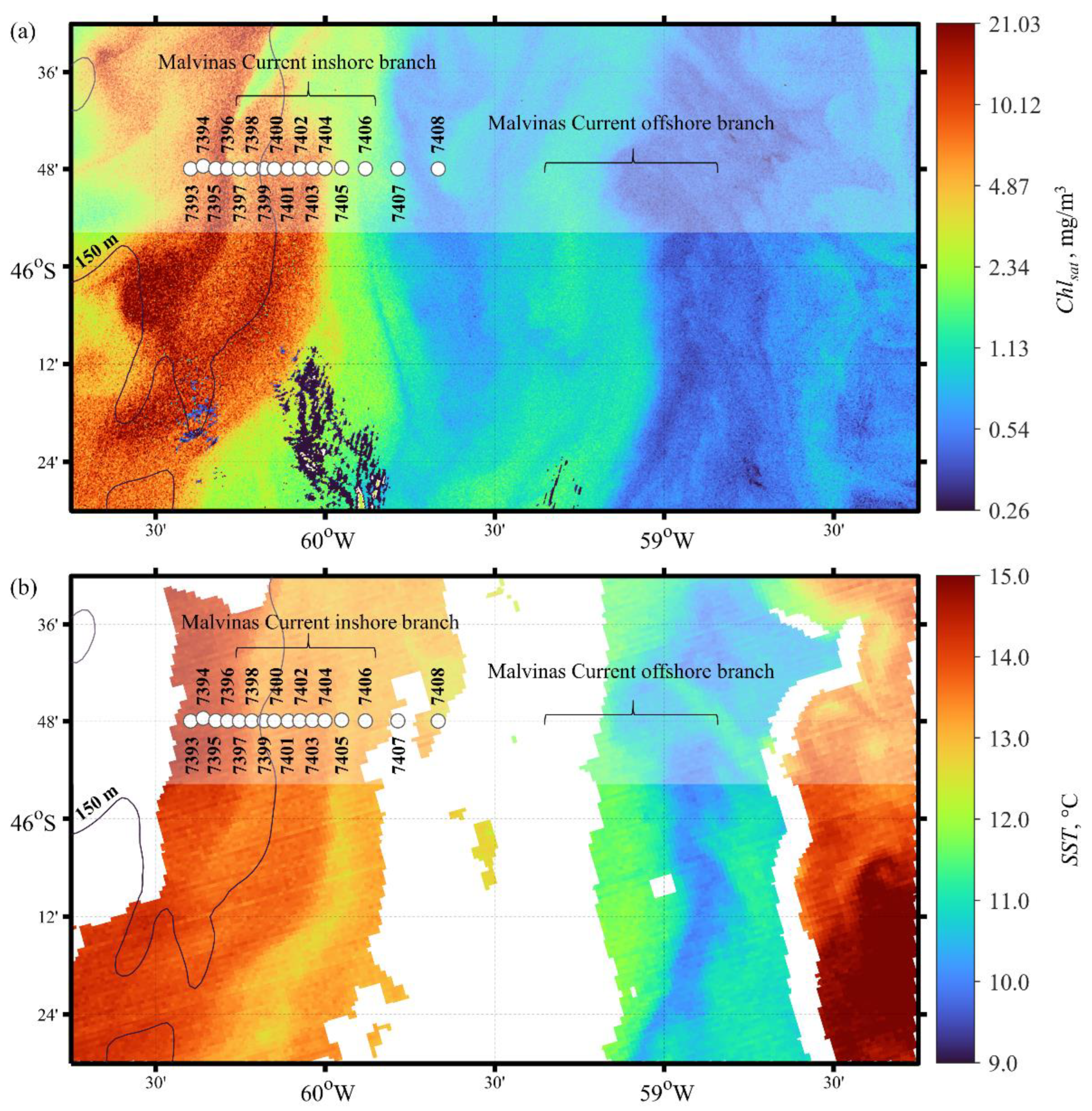
2.3. Satellite Sea Surface Temperature and Chlorophyll-a
2.4. Simulated Oceanographic Data and Bottom Topography
3. Results
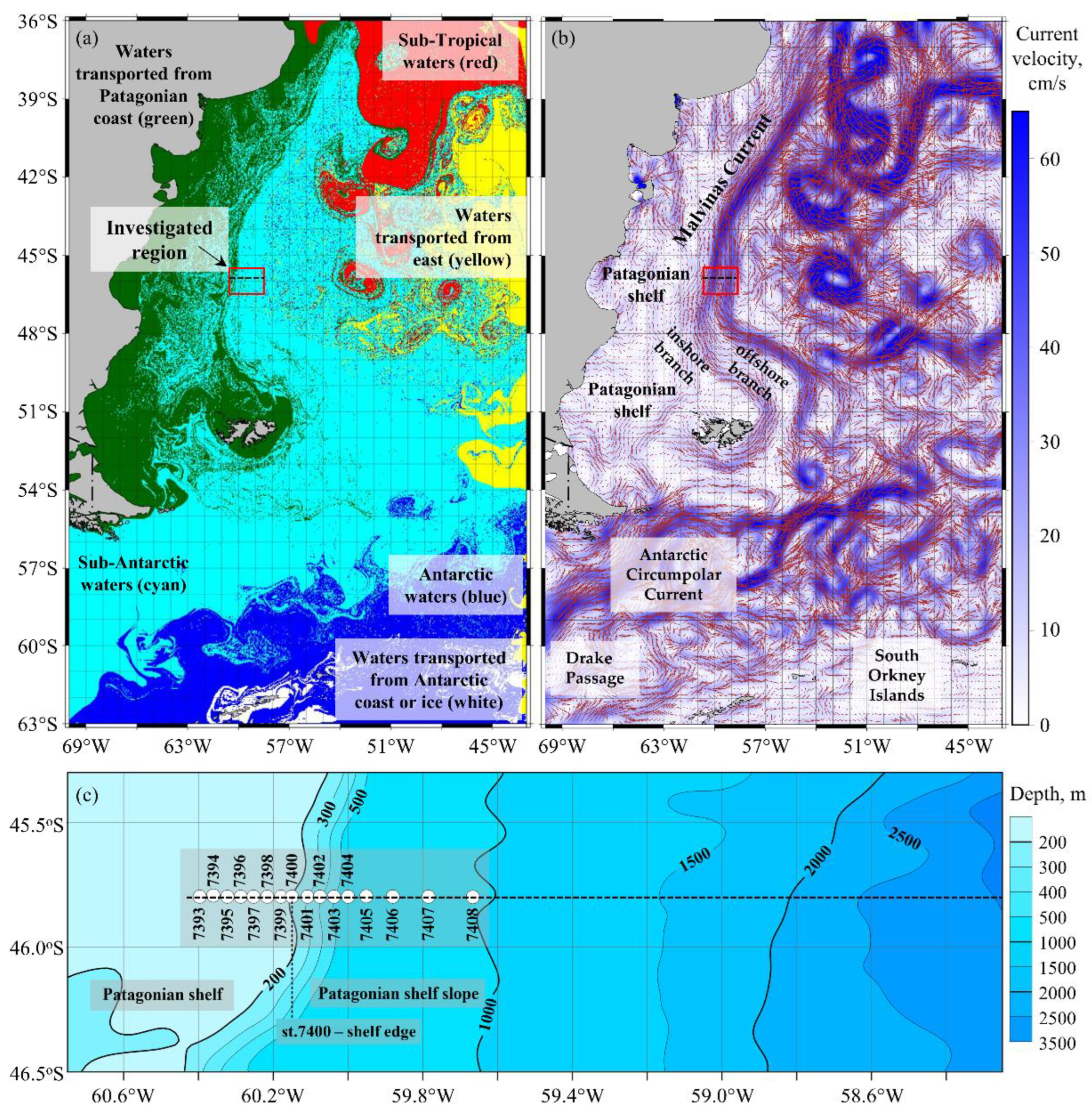
3.1. Common Oceanographic and Bio-Optical Characteristics of the Study Site
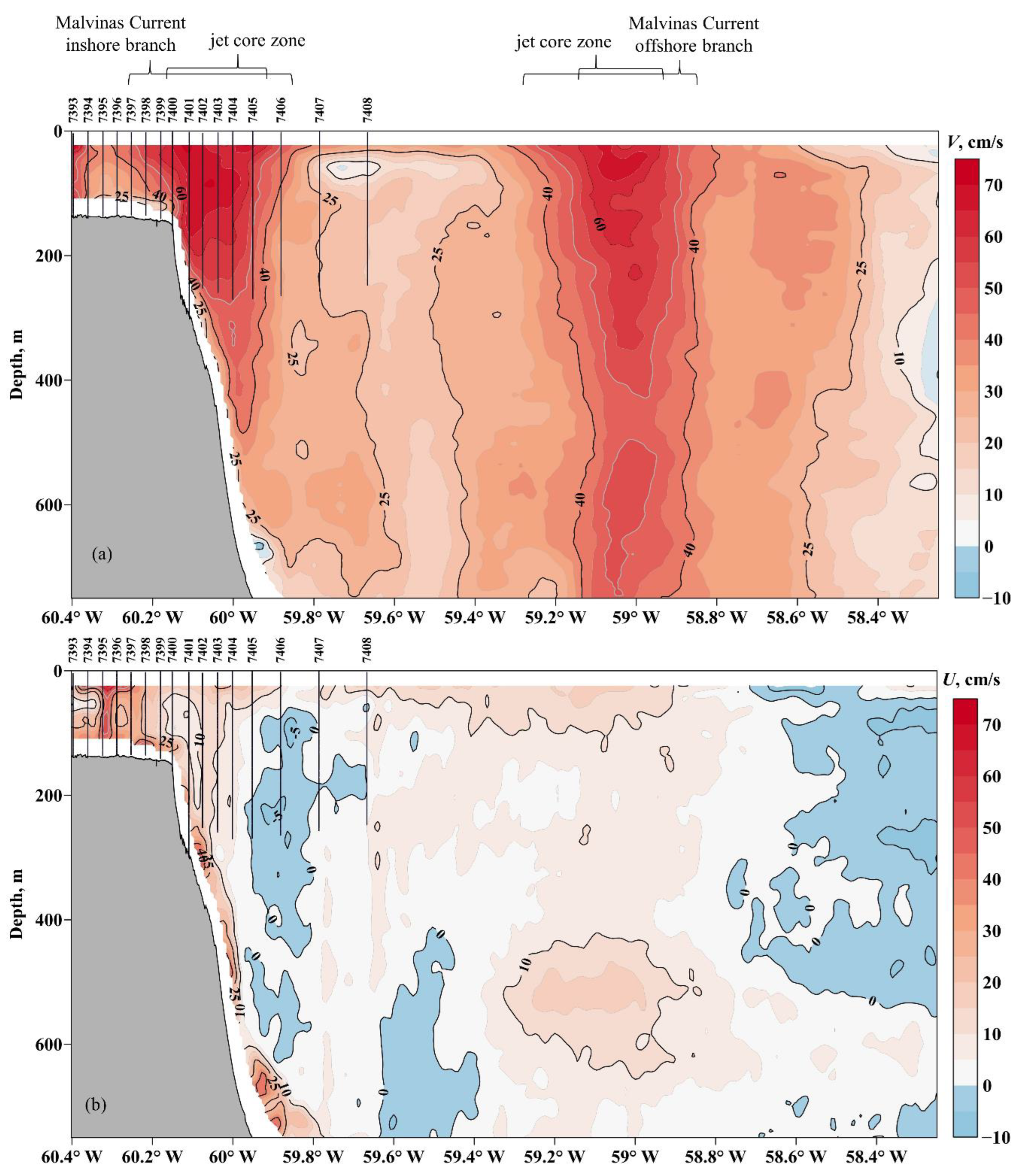
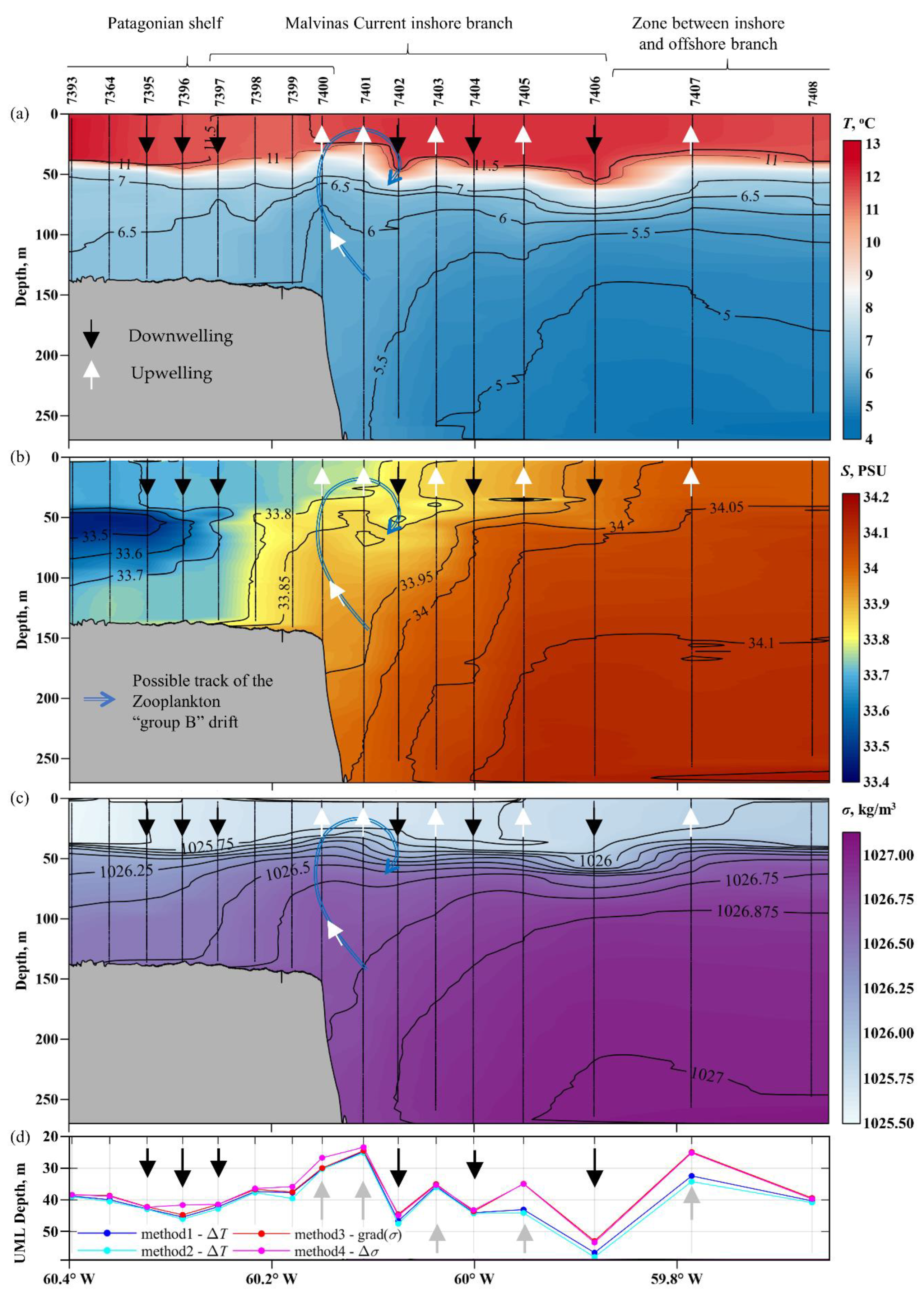
3.2. Oceanographic Variables
3.3. Biooptical Characteristics
3.4. Water Mass Classification
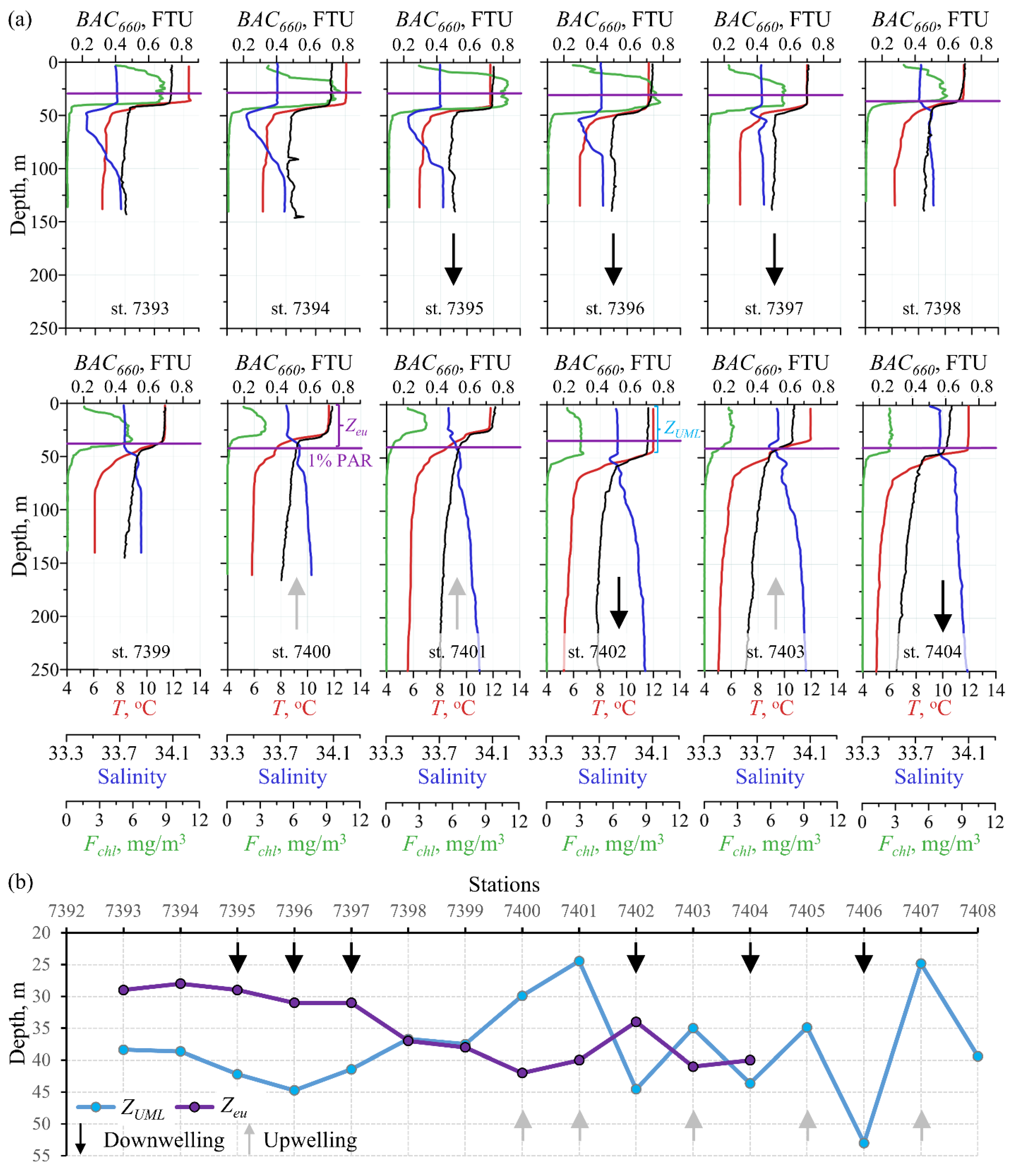
3.5. Variations in the Euphotic Depth and the Upper Mixel Layer Depth
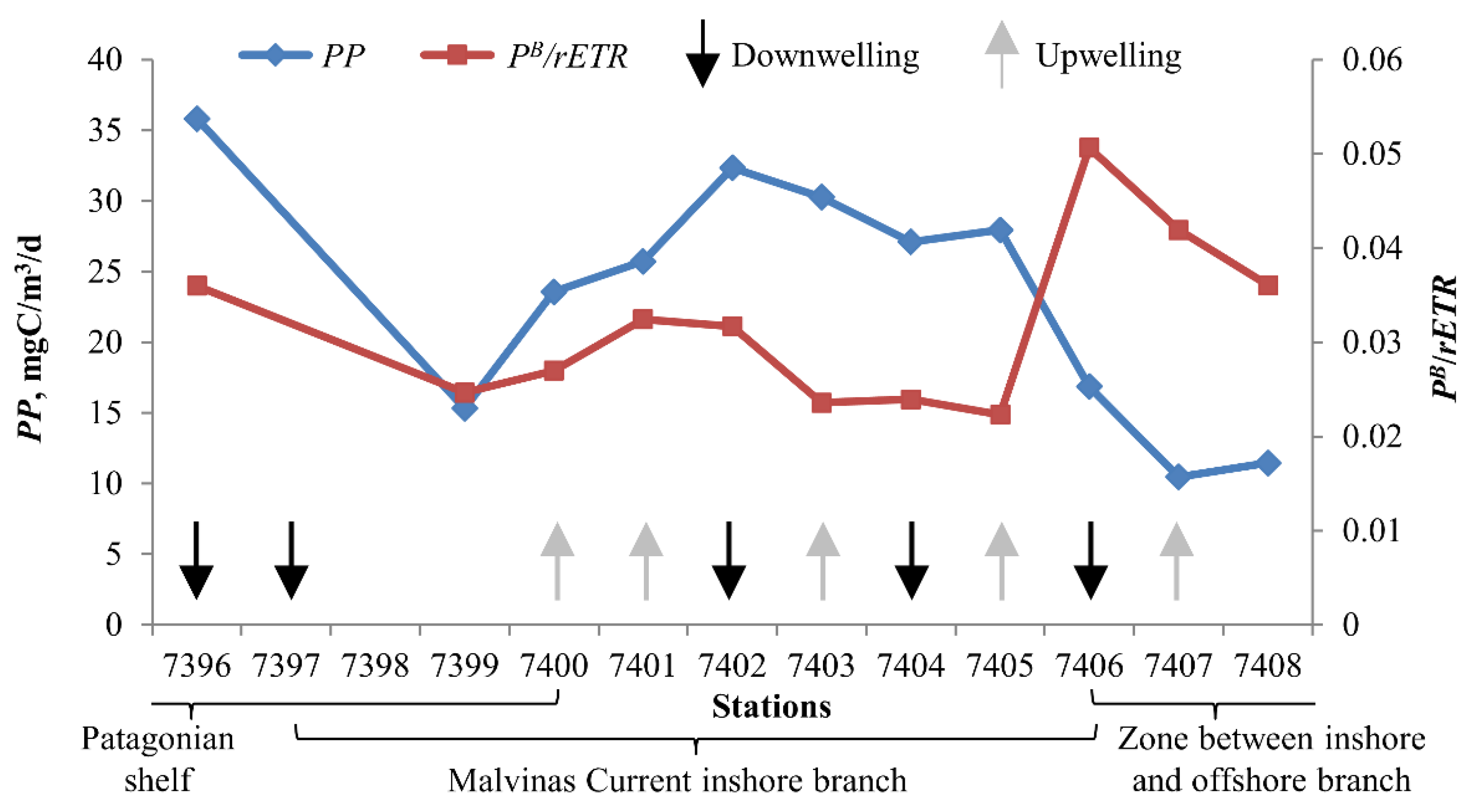
3.6. Phytoplankton Biological Activity
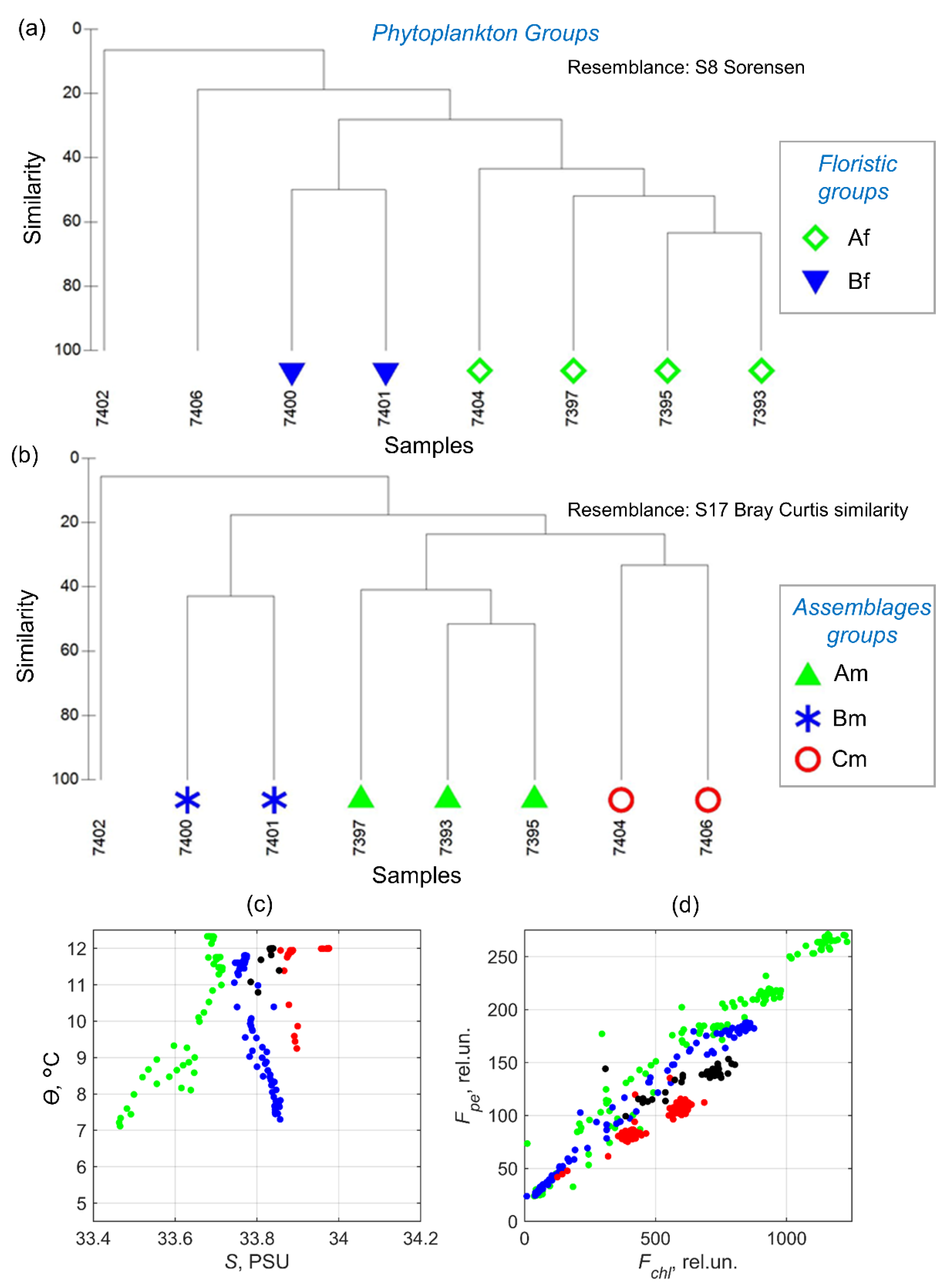
3.7. Phytoplankton Communities
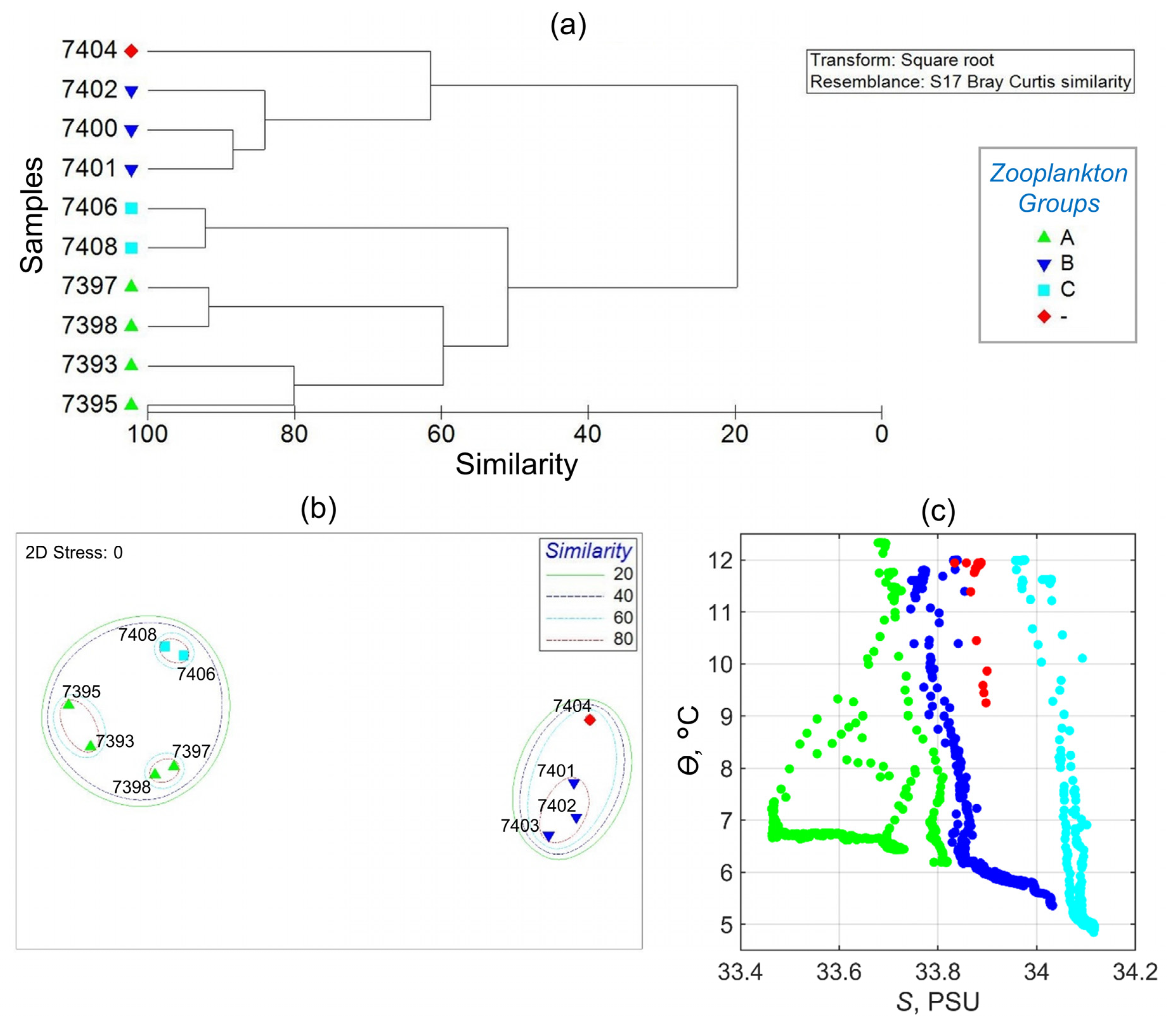
3.8. Zooplankton Species
3.9. Observations of Marine Mammals and Sea Birds
4. Discussion
4.1. Types of Water Masses and Hydrodynamic Manifestations of Oceanographic Characteristics
4.2. Relation between the Depths of the Upper Mixed and Euphotic Zones
4.3. Analysis of Photosynthetic Activity of Phytoplankton
4.4. Phytoplankton Communities
4.5. Zooplankton Communities
4.6. Observations of Marine Mammals and Sea Birds
4.7. Summary Information about Hydro-Physical and Biological Charactristics
5. Conclusions
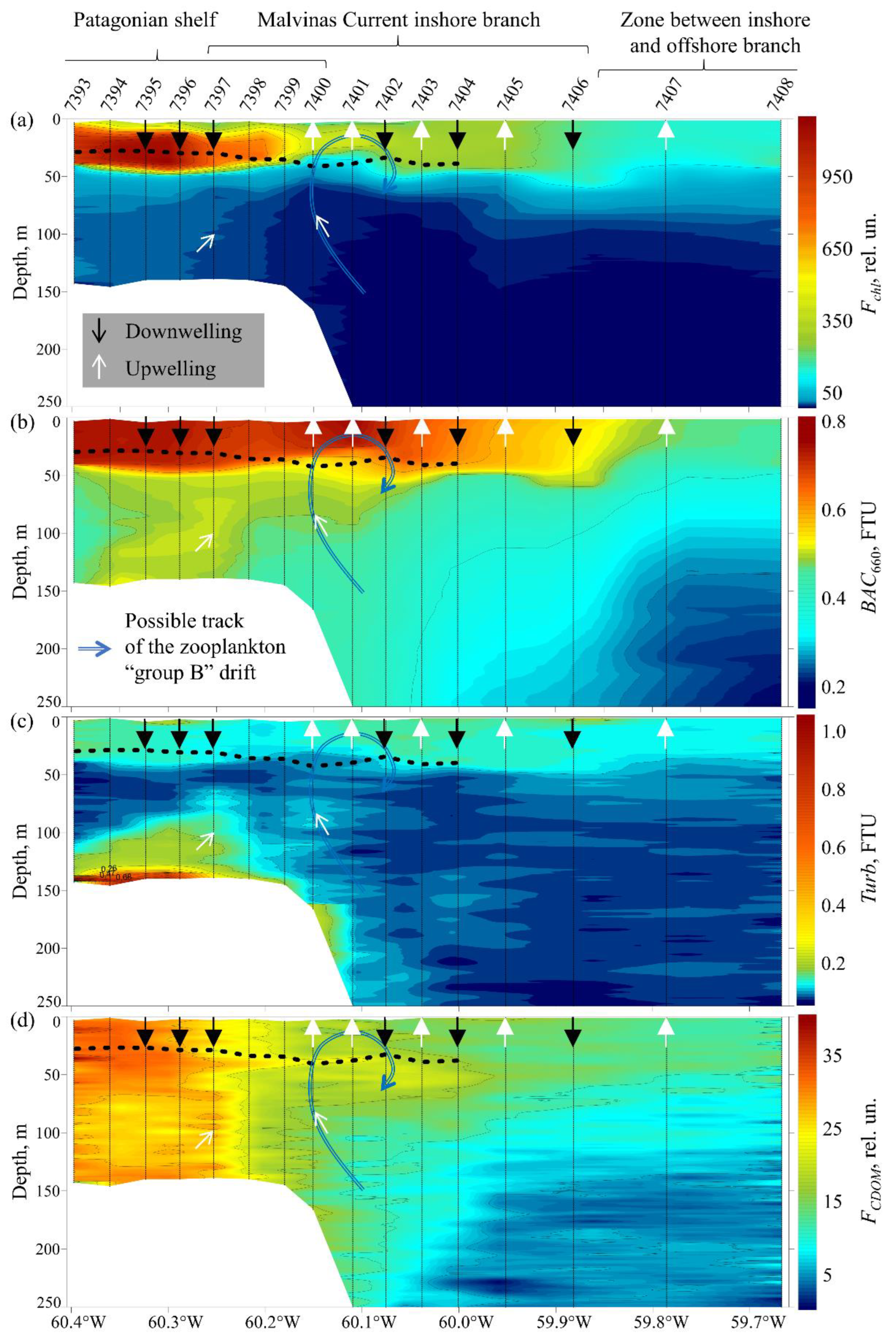
- Sub-mesoscale structure of alternating upwellings and downwellings in the upper mixed layer has been identified in the region of the outer Patagonian Shelf and inshore branch of the Malvinas Current along ~46° S section.
- In general, the differences in the upper mixed layer thickness between identified upwelling and downwelling zones are significant. In the first case, they are in the range of ~25–35 m, and in the second case, in the range of 40–55 m.
- The euphotic zone is larger in upwelling zones and smaller in downwelling zones. The difference can be as high as 6–10 m in adjacent upwelling and downwelling zones.
- Phytoplankton photosynthetic efficiency increases during the changeover between upwelling and downwelling.
- Distribution of all considered biological communities of different trophic levels is similar in accordance with the identified oceanographic features.
- Most of the phytoplankton species list was formed by dinoflagellates, among which heterotrophic forms prevailed. In quantitative terms, the pyramimonad Prasinoderma coloniale, a coccoid representative of picoplankton, dominated everywhere. Two floristic and three assemblage groups were distinguished among the communities. Biodiversity was high above the Patagonian Shelf and low above the shelf edge and in the core of Malvinas Current inshore branch.
- Zooplankton was mostly dominated by copepods. Subantarctic species/taxa of zooplankton concentrated in the nearshore waters of the Patagonian Shelf, while Antarctic species/taxa were most abundant in the zone between the inshore and offshore branches of the MC.
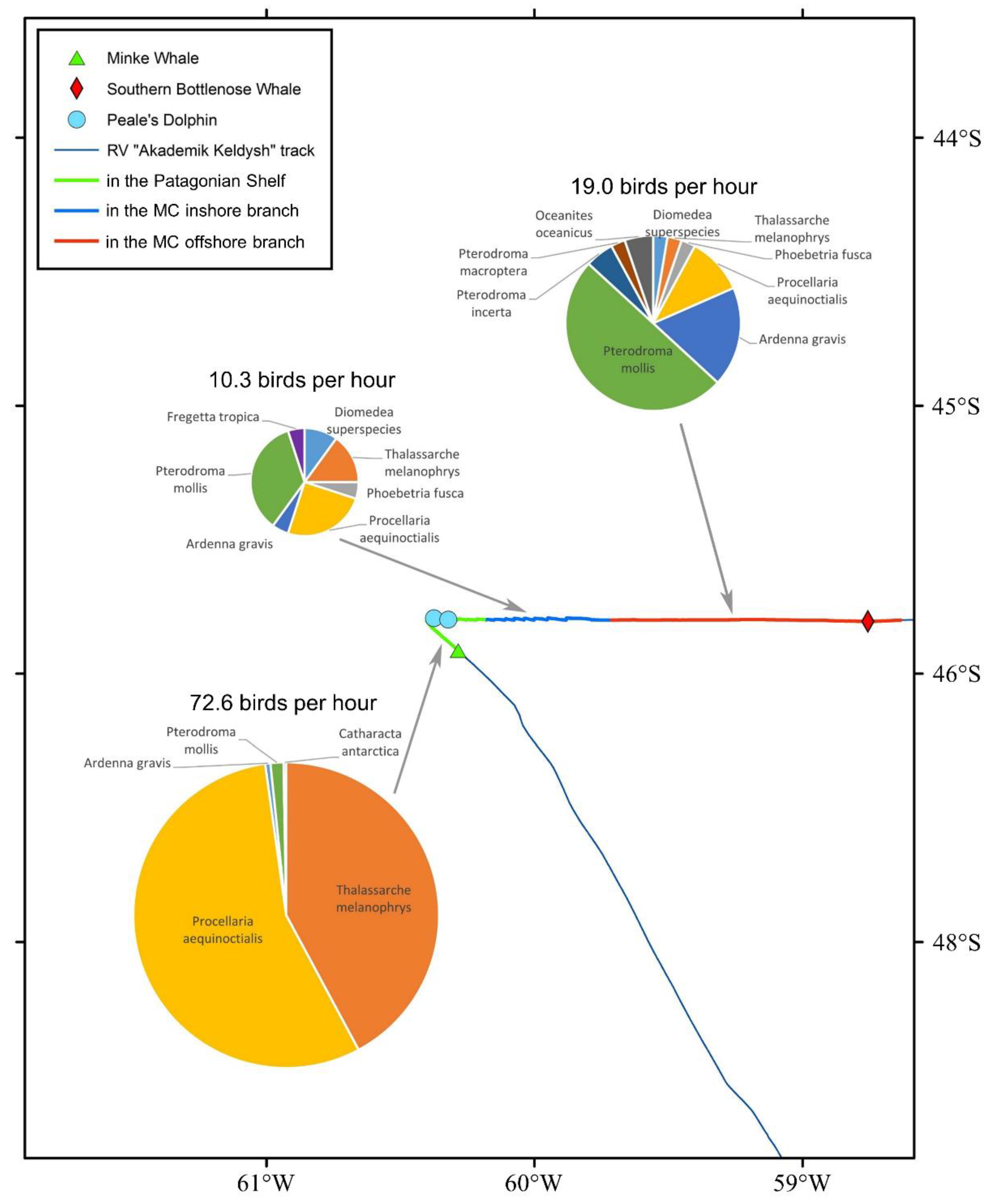
- The distribution of birds and mammals is different in the waters of shelf and Malvinas Current; the relative abundance of birds is minimal in the inshore branch of the Malvinas Current, where the strongest upwelling was identified.
Author Contributions
Funding
Institutional Review Board Statement
Informed Consent Statement
Data Availability Statement
Conflicts of Interest
References
- Hoffmeyer, M.; Sabatini, M.; Brandini, F.; Calliari, D.; Santinelli, N. (Eds.) Plankton Ecology of the Southwestern Atlantic: From the Subtropical to the Subantarctic Realm; Springer: Cham, Switzerland, 2018; p. 586. [Google Scholar] [CrossRef]
- Peterson, R.G.; Whitworth, T. The Subantarctic and Polar Fronts in Relation to Deep Water Masses through the Southwestern Atlantic. J. Geophys. Res. 1989, 94, 10817. [Google Scholar] [CrossRef]
- Franco, B.C.; Piola, A.R.; Rivas, A.L.; Baldoni, A.; Pisoni, J.P. Multiple Thermal Fronts near the Patagonian Shelf Break. Geophys. Res. Lett. 2008, 35, L02607. [Google Scholar] [CrossRef] [Green Version]
- Piola, A.R.; Franco, B.C.; Palma, E.D.; Saraceno, M. Multiple Jets in the Malvinas Current. J. Geophys. Res. Ocean. 2013, 118, 2107–2117. [Google Scholar] [CrossRef] [Green Version]
- Frey, D.I.; Piola, A.R.; Krechik, V.A.; Fofanov, D.V.; Morozov, E.G.; Silvestrova, K.P.; Tarakanov, R.Y.; Gladyshev, S.V. Direct Measurements of the Malvinas Current Velocity Structure. J. Geophys. Res. Ocean. 2021, 126, e2020JC016727. [Google Scholar] [CrossRef]
- Artana, C.; Provost, C.; Poli, L.; Ferrari, R.; Lellouche, J. Revisiting the Malvinas Current Upper Circulation and Water Masses Using a High-Resolution Ocean Reanalysis. J. Geophys. Res. Ocean. 2021, 126, e2021JC017271. [Google Scholar] [CrossRef]
- Paniagua, G.F.; Saraceno, M.; Piola, A.R.; Charo, M.; Ferrari, R.; Artana, C.; Provost, C. Malvinas Current at 44.7° S: First Assessment of Velocity Temporal Variability from in Situ Data. Prog. Oceanogr. 2021, 195, 102592. [Google Scholar] [CrossRef]
- Palma, E.D.; Matano, R.P.; Piola, A.R. A Numerical Study of the Southwestern Atlantic Shelf Circulation: Stratified Ocean Response to Local and Offshore Forcing. J. Geophys. Res. 2008, 113, C11010. [Google Scholar] [CrossRef]
- Piola, A.R.; Avellaneda, N.M.; Guerrero, R.A.; Jardón, F.P.; Palma, E.D.; Romero, S.I. Malvinas-Slope Water Intrusions on the Northern Patagonia Continental Shelf. Ocean. Sci. 2010, 6, 345–359. [Google Scholar] [CrossRef] [Green Version]
- Matano, R.P.; Palma, E.D.; Piola, A.R. The Influence of the Brazil and Malvinas Currents on the Southwestern Atlantic Shelf Circulation. Ocean. Sci. 2010, 6, 983–995. [Google Scholar] [CrossRef]
- Acha, E.M.; Mianzan, H.W.; Guerrero, R.A.; Favero, M.; Bava, J. Marine Fronts at the Continental Shelves of Austral South America. J. Mar. Syst. 2004, 44, 83–105. [Google Scholar] [CrossRef]
- Miloslavich, P.; Klein, E.; Díaz, J.M.; Hernández, C.E.; Bigatti, G.; Campos, L.; Artigas, F.; Castillo, J.; Penchaszadeh, P.E.; Neill, P.E.; et al. Marine Biodiversity in the Atlantic and Pacific Coasts of South America: Knowledge and Gaps. PLoS ONE 2011, 6, e14631. [Google Scholar] [CrossRef] [PubMed] [Green Version]
- Matano, R.P.; Palma, E.D. On the Upwelling of Downwelling Currents. J. Phys. Oceanogr. 2008, 38, 2482–2500. [Google Scholar] [CrossRef]
- Valla, D.; Piola, A.R. Evidence of Upwelling Events at the Northern Patagonian Shelf Break. J. Geophys. Res. Ocean. 2015, 120, 7635–7656. [Google Scholar] [CrossRef]
- Carranza, M.M.; Gille, S.T.; Piola, A.R.; Charo, M.; Romero, S.I. Wind Modulation of Upwelling at the Shelf-Break Front off Patagonia: Observational Evidence. J. Geophys. Res. Ocean. 2017, 122, 2401–2421. [Google Scholar] [CrossRef]
- Garcia, V.M.T.; Garcia, C.A.E.; Mata, M.M.; Pollery, R.C.; Piola, A.R.; Signorini, S.R.; McClain, C.R.; Iglesias-Rodriguez, M.D. Environmental Factors Controlling the Phytoplankton Blooms at the Patagonia Shelf-Break in Spring. Deep. Sea Res. Part I Oceanogr. Res. Pap. 2008, 55, 1150–1166. [Google Scholar] [CrossRef]
- Rivas, A.L.; Dogliotti, A.I.; Gagliardini, D.A. Seasonal Variability in Satellite-Measured Surface Chlorophyll in the Patagonian Shelf. Cont. Shelf Res. 2006, 26, 703–720. [Google Scholar] [CrossRef]
- Romero, S.I.; Piola, A.R.; Charo, M.; Garcia, C.A.E. Chlorophyll- a Variability off Patagonia Based on SeaWiFS Data. J. Geophys. Res. 2006, 111, C05021. [Google Scholar] [CrossRef]
- Salyuk, P.A.; Glukhovets, D.I.; Lipinskaya, N.A.; Moiseeva, N.A.; Churilova, T.Y.; Ponomarev, V.I.; Aglova, E.A.; Artemiev, V.A.; Latushkin, A.A.; Major, A.Y. Variability of the Sea Surface Bio-Optical Characteristics in the Region of Falkland Current and Patagonian Shelf. Sovrem. Probl. Distantsionnogo Zondirovaniya Zemli Iz Kosm. 2021, 18, 200–213. [Google Scholar] [CrossRef]
- Pakhomov, E.; Pshenichnov, L.; Krot, A.; Paramonov, V.; Slypko, I.; Zabroda, P. Zooplankton distribution and community structure in the Pacific and Atlantic Sectors of the Southern Ocean during austral summer 2017–2018: A Pilot Study Conducted from Ukrainian Long–Liners. J. Mar. Sci. Eng. 2020, 8, 488. [Google Scholar] [CrossRef]
- Turner, J.T. The importance of small planktonic copepods and their roles in pelagic marine food webs. Zool. Stud. 2004, 43, 255–266. [Google Scholar]
- Von Dassow, P.; Montresor, M. Unveiling the Mysteries of Phytoplankton Life Cycles: Patterns and Opportunities behind Complexity. J. Plankton Res. 2011, 33, 3–12. [Google Scholar] [CrossRef] [Green Version]
- Otto, S.A.; Niiranen, S.; Blenckner, T.; Tomczak, M.T.; Müller-Karulis, B.; Rubene, G.; Möllmann, C. Life Cycle Dynamics of a Key Marine Species Under Multiple Stressors. Front. Mar. Sci. 2020, 7. [Google Scholar] [CrossRef]
- Barton, A.D.; Irwin, A.J.; Finkel, Z.V.; Stock, C.A. Anthropogenic Climate Change Drives Shift and Shuffle in North Atlantic Phytoplankton Communities. Proc. Natl. Acad. Sci. USA 2016, 113, 2964–2969. [Google Scholar] [CrossRef] [PubMed] [Green Version]
- Franco, B.C.; Defeo, O.; Piola, A.R.; Barreiro, M.; Yang, H.; Ortega, L.; Gianelli, I.; Castello, J.P.; Vera, C.; Buratti, C.; et al. Climate Change Impacts on the Atmospheric Circulation, Ocean, and Fisheries in the Southwest South Atlantic Ocean: A Review. Clim. Chang. 2020, 162, 2359–2377. [Google Scholar] [CrossRef]
- Nievas El Makte, M.L.; Polifroni, R.; Sepúlveda, M.A.; Fazio, A. Petroleum Hydrocarbons in Atlantic Coastal Patagonia. In Anthropogenic Pollution of Aquatic Ecosystems; Häder, D.P., Helbling, E.W., Villafañe, V.E., Eds.; Springer: Cham, Switzerland, 2021; pp. 325–352. [Google Scholar] [CrossRef]
- Goni, G.J.; Bingas, F.; DiNezio, P.N. Observed low frequency variability of the Brazil Current front. J. Geophys. Res. Ocean. 2011, 116, C10037. [Google Scholar] [CrossRef] [Green Version]
- Combes, V.; Matano, R.P. Trends in the Brazil/Malvinas confluence region. Geophys. Res. Lett. 2014, 41, 8971–8977. [Google Scholar] [CrossRef]
- Franco, B.; Ruiz-Etcheverry, L.; Marrari, M.; Piola, A.; Matano, R. Climate Change Impacts on the Patagonian Shelf Break Front. Geophys. Res. Lett. 2022, 49, e2021GL096513. [Google Scholar] [CrossRef]
- Helbling, E.W.; Narvarte, M.A.; González, R.A.; Villafañe, V.E. (Eds.) Global Change in Atlantic Coastal Patagonian Ecosystems; Springer: Cham, Switzerland, 2022; p. 463. [Google Scholar] [CrossRef]
- Chereskin, T.K.; Harris, C.L. Shipboard Acoustic Doppler Current Profiling during the WOCE Indian Ocean Expedition: I10; Scripps Institution of Oceanography, University of California: San Diego, CA, USA, 1997. [Google Scholar]
- Egbert, G.D.; Erofeeva, S.Y. Efficient Inverse Modeling of Barotropic Ocean Tides. J. Atmos. Ocean. Technol. 2002, 19, 183–204. [Google Scholar] [CrossRef]
- Monterey, G.I.; Levitus, S. Seasonal variability of mixed layer depth for the world ocean. NOAA Atlas NESDIS 1997, 14, 96. [Google Scholar]
- Kara, A.B.; Rochford, P.A.; Hurlburt, H.E. An optimal definition for ocean mixed layer depth. J. Geophys. Res. 2000, 105, 16803–16821. [Google Scholar] [CrossRef]
- Brainerd, K.E.; Gregg, M.C. Surface mixed and mixing layer depths. Deep. Sea Res. Part I Oceanogr. Res. Pap. 1995, 42, 1521–1543. [Google Scholar] [CrossRef]
- deBoyer Montégut, C.; Madec, G.; Fischer, A.S.; Lazar, A.; Ludicone, D. Mixed layer depth over the global ocean: An examination of profile data and a profile-based climatology. J. Geophys. Res. 2004, 109. [Google Scholar] [CrossRef] [Green Version]
- Nielsen, E.S. The Use of Radio-Active Carbon (C14) for Measuring Organic Production in the Sea. ICES J. Mar. Sci. 1952, 18, 117–140. [Google Scholar] [CrossRef]
- Intergovernmental Oceanographic Commission. Protocols for the Joint Global Ocean Flux Study (JGOFS) Core Measurements. In Intergovernmental Oceanographic Commission Manuals and Guides, 29; UNESCO-IOC: Paris, France, 1994; p. 170. [Google Scholar] [CrossRef]
- Mosharov, S.A.; Sergeeva, V.M.; Kremenetskiy, V.V.; Sazhin, A.F.; Stepanova, S.V. Assessment of Phytoplankton Photosynthetic Efficiency Based on Measurement of Fluorescence Parameters and Radiocarbon Uptake in the Kara Sea. Estuar. Coast. Shelf Sci. 2019, 218, 59–69. [Google Scholar] [CrossRef]
- Hoppe, C.J.M.; Klaas, C.; Osserbaar, S.; Soppa, M.A.; Cheah, W.; Laglera, L.M.; Santos-Echeandia, J.; Rost, B.; Wolf-Gladrow, D.A.; Bracher, A.; et al. Controls of primary production in two phytoplankton blooms in the Antarctic Circumpolar Current. Deep.-Sea Res. II 2017, 138, 63–73. [Google Scholar] [CrossRef] [PubMed] [Green Version]
- Genty, B.; Briantais, J.-M.; Baker, N.R. The Relationship between the Quantum Yield of Photosynthetic Electron Transport and Quenching of Chlorophyll Fluorescence. Biochim. Et Biophys. Acta (BBA)-Gen. Subj. 1989, 990, 87–92. [Google Scholar] [CrossRef]
- Schreiber, U. Pulse-Amplitude-Modulation (PAM) Fluorometry and Saturation Pulse Method: An Overview. In Chlorophyll a Fluorescence. Advances in Photosynthesis and Respiration, vol 19; Papageorgiou, G.C., Govindjee, Eds.; Springer: Dordrecht, The Netherlands, 2004; pp. 279–319. [Google Scholar] [CrossRef]
- Napoleon, C.; Raimbault, V.; Claquin, P. Influence of nutrient stress on the relationships between PAM measurements and carbon incorporation in four phytoplankton species. PLoS ONE 2013, 8, e66423. [Google Scholar] [CrossRef] [PubMed]
- Hannam, G. Relative abundance and distribution of phytoplankton in Glacier Bay, Alaska. In Proceedings from the University of Washington School of Oceanography Undergraduate Thesis Research Expedition to Glacier Bay Alaska, March 2008; Keil, R., Kelley, D., D’Asaro, E., Krembs, C., Collins, R.E., Eds.; School of Oceanography, University of Washington: Seattle, WA, USA, 2008; p. 14. [Google Scholar]
- Lim, H.C.; Teng, S.T.; Leaw, C.P.; Wataki, M.; Lim, P. Phytoplankton assemblage of the Merambong Shoal, Tebrau Straits with note on potentially harmful species. Malay Nat. J. 2014, 66, 198–221. [Google Scholar]
- Horner, R. A Taxonomic Guide to Some Common Marine Phytoplankton; Biopress Limited: Bristol, England, 2002; pp. 1–110. [Google Scholar]
- Dodge, J.; Hermes, H. A Revision of the Diplopsalis Group of Dinoflagellates (Dinophyceae) Based on Material from the British Isles. Bot. J. Linn. Soc. 1981, 83, 15–26. [Google Scholar] [CrossRef]
- Scott, F.J.; Marchant, H.J. (Eds.) Antarctic Marine Protists. Australian Biological Resources Study, Canberra and Australian Antarctic Division; Australian Antarctic Division: Hobart, Australia, 2005; p. 563. [Google Scholar]
- Okolodkov, Y.B. Protoperidinium Bergh (Dinoflagellata) in the Southeastern Mexican Pacific Ocean: Part I. Bot. Mar. 2005, 48, 284–296. [Google Scholar] [CrossRef]
- Okolodkov, Y.B. Protoperidinium Bergh (Dinophyceae) of the National Park Sistema Arrecifal Veracruzano, Gulf of Mexico, with a Key for Identification. Acta Bot. Mex. 2008, 84, 93–149. [Google Scholar] [CrossRef]
- Pienaar, R.N.; Sakai, H.; Horiguchi, T. Description of a New Dinoflagellate with a Diatom Endosymbiont, Durinskia capensis Sp. Nov. (Peridiniales, Dinophyceae) from South Africa. J. Plant Res. 2007, 120, 247. [Google Scholar] [CrossRef] [PubMed]
- Al-Kandari, M.; Al-Yamani, F.; Al-Rifaie, K. Marine Phytoplankton Atlas of Kuwait’s Waters; Kuwait Institute for Scientific Research: Safat, Kuwait, 2009; p. 351. [Google Scholar]
- Myat, S.; Thaw, M.S.H.; Matsuoka, K.; Lay, K.K.; Koike, K. Phytoplankton surveys off the southern Myanmar coast of the Andaman Sea: An emphasis on dinoflagellates including potentially harmful species. Fish. Sci. 2012, 78, 1091–1106. [Google Scholar] [CrossRef]
- Gul, S.; Nawaz, M.F. The Dinoflagellate Genera Protoperidinium and Podolampas from Pakistan’s shelf and deep sea vicinity (North Arabian Sea). Turk. J. Fish. Aquat. Sci. 2014, 14, 91–100. [Google Scholar] [CrossRef] [PubMed]
- Estrada, M.; Delgado, M.; Blasco, D.; Latasa, M.; Cabello, A.M.; Benítez-Barrios, V.; Fraile-Nuez, E.; Mozetič, P.; Vidal, M. Phytoplankton across Tropical and Subtropical Regions of the Atlantic, Indian and Pacific Oceans. PLoS ONE 2016, 11, e0151699. [Google Scholar] [CrossRef] [Green Version]
- Kretschmann, J.; Čalasan, A.Ž.; Gottschling, M. Molecular Phylogenetics of Dinophytes Harboring Diatoms as Endosymbionts (Kryptoperidiniaceae, Peridiniales), with Evolutionary Interpretations and a Focus on the Identity of Durinskia Oculata from Prague. Mol. Phylogenetics Evol. 2018, 118, 392–402. [Google Scholar] [CrossRef]
- Phan-Tan, L.; Nguyen-Ngoc, L.; Doan-Nhu, H.; Raine, R.; Larsen, J. Species diversity of Protoperidinium sect. Oceanica (Dinophyceae, Peridiniales) in Vietnamese waters, with description of the new species P. larsenii sp. nov. Nord. J. Bot. 2017, 35, 129–146. [Google Scholar] [CrossRef]
- Furuya, K.; Mitsunori, I.; Po Teen, L.; Songhui, L.; Chui-Pin, L.; Azanza, R.V.; Kim, H.-G.; Fukuyo, Y. Overview of harmful algal blooms in Asia. In Global Ecology and Oceanography of Harmful Algal Blooms. Ecological Studies; Glibert, P., Berdalet, E., Burford, M., Pitcher, G., Zhou, M., Eds.; Springer: Cham, Switzerland, 2018; Volume 232, pp. 289–308. [Google Scholar] [CrossRef]
- Weikert, H.; John, H.-C. Experiences with a Modified Bé Multiple Opening-Closing Plankton Net. J. Plankton Res. 1981, 3, 167–176. [Google Scholar] [CrossRef]
- Bouchard, S.; Cote, S.; St-Jacques, J.; Robillard, G.; Renaud, P. Effectiveness of Virtual Reality Exposure in the Treatment of Arachnophobia Using 3D Games. Technol. Health Care 2006, 14, 19–27. [Google Scholar] [CrossRef]
- Razouls, C.; Desreumaux, N.; Kouwenberg, J.; de Bovee, F. Biodiversity of Marine Planktonic Copepods (Morphology, Geographical Distribution and Biological Data); Sorbonne University, CNRS: Paris, France, 2022; Available online: http://copepodes.obs-banyuls.fr/en (accessed on 23 May 2022).
- Boltovskoy, D. Radiolaria Polycystina. South Atl. Zooplankton 1999, 1, 149–212. [Google Scholar]
- WoRMS Editorial Board. World Register of Marine Species. 2015. Available online: http://www.marinespecies.org (accessed on 22 May 2022).
- Goswami, S.C. Zooplankton Methodology Collection and Identification-a Field Manual: National Institute of Oceanography; Dhargalkar, V.K., Verlecar, X.N., Eds.; National Institute of Oceanography: Panaji, India, 2004; pp. 5–8. [Google Scholar]
- Clarke, K.R.; Warwick, R.M.; Marine, P. Change in Marine Communities: An Approach to Statistical Analysis and Interpretation, 2nd ed.; PRIMER-E: Plymouth, UK, 2001. [Google Scholar]
- Prants, S.V. Backward-in-Time Methods to Simulate Large-Scale Transport and Mixing in the Ocean. Phys. Scr. 2015, 90, 074054. [Google Scholar] [CrossRef]
- Bowers, D.G.; Brett, H.L. The relationship between CDOM and salinity in estuaries: An analytical and graphical solution. J. Mar. Syst. 2008, 73, 1–7. [Google Scholar] [CrossRef]
- Stedmon, C.A.; Osburn, C.L.; Kragh, T. Tracing water mass mixing in the Baltic–North Sea transition zone using the optical properties of coloured dissolved organic matter. Estuar. Coast. Shelf Sci. 2010, 87, 156–162. [Google Scholar] [CrossRef]
- Fransz, H.G. Vernal Abundance, Structure and Development of Epipelagic Copepod Populations of the Eastern Weddell Sea (Antarctica). Polar Biol. 1988, 9, 107–114. [Google Scholar] [CrossRef]
- Foster, B.A. Time and Depth Comparisons of Sub-Ice Zooplankton in McMurdo Sound, Antarctica. Polar Biol. 1989, 9, 431–435. [Google Scholar] [CrossRef]
- Piola, A.R.; Matano, R.P.; Steele, J.H.; Thorpe, S.A.; Turekian, K.K. Brazil and Falklands (Malvinas) currents. In Ocean Currents, Encyclopedia Ocean Sciences; Steele, J.H., Thorpe, S.A., Turekian, K.K., Eds.; Academia Press: Cambridge, MA, USA, 2010; pp. 35–43. [Google Scholar] [CrossRef]
- Ehrlich, M.D.; Sánchez, R.P.; De Ciechomski, J.D.; Machinandiarena, L.; Pájaro, M. Ichthyoplankton composition, distribution and abundance on the southern patagonian shelf and adjacent waters. INIDEP Doc. Científico 1999, 5, 37–65. Available online: http://hdl.handle.net/1834/2574 (accessed on 19 November 2022).
- Carreto, J.I.; Montoya, N.G.; Carignan, M.O.; Akselman, R.; Acha, E.M.; Derisio, C. Environmental and Biological Factors Controlling the Spring Phytoplankton Bloom at the Patagonian Shelf-Break Front–Degraded Fucoxanthin Pigments and the Importance of Microzooplankton Grazing. Prog. Oceanogr. 2016, 146, 1–21. [Google Scholar] [CrossRef] [Green Version]
- Morozov, E.G.; Tarakanov, R.Y.; Demidova, T.A.; Frey, D.I.; Makarenko, N.I.; Remeslo, A.V.; Gritsenko, A.M. Velocity and transport of the Falkland Current at 46°S. Russ. J. Earth Sci. 2016, 16, ES6005. [Google Scholar] [CrossRef]
- Artana, C.; Provost, C.; Lellouche, J.M.; Rio, M.H.; Ferrari, R.; Sennéchael, N. The Malvinas current at the confluence with the Brazil current: Inferences from 25 years of Mercator ocean reanalysis. J. Geophys. Res. Ocean. 2019, 124, 7178–7200. [Google Scholar] [CrossRef]
- Sabatini, M.; Reta, R.; Matano, R. Circulation and Zooplankton Biomass Distribution over the Southern Patagonian Shelf during Late Summer. Cont. Shelf Res. 2004, 24, 1359–1373. [Google Scholar] [CrossRef]
- Karabashev, G.S.; Evdoshenko, M.A. Narrowband shortwave minima of multispectral reflectance as indication of algal blooms associated with the mesoscale variability in the Brazil-Malvinas Confluence. Oceanologia 2018, 60, 527–543. [Google Scholar] [CrossRef]
- Baldry, K.; Strutton, P.G.; Hill, N.A.; Boyd, P.W. Subsurface chlorophyll-a maxima in the Southern Ocean. Front. Mar. Sci. 2020, 7, 671. [Google Scholar] [CrossRef]
- Ardyna, M.; Babin, M.; Gosselin, M.; Devred, E.; Bélanger, S.; Matsuoka, A.; Tremblay, J.É. Parameterization of vertical chlorophyll a in the Arctic Ocean: Impact of the subsurface chlorophyll maximum on regional, seasonal, and annual primary production estimates. Biogeosciences 2013, 10, 4383–4404. [Google Scholar] [CrossRef] [Green Version]
- Lavigne, H.; D’ortenzio, F.; Ribera D’Alcalà, M.; Claustre, H.; Sauzède, R.; Gacic, M. On the vertical distribution of the chlorophyll a concentration in the Mediterranean Sea: A basin-scale and seasonal approach. Biogeosciences 2015, 12, 5021–5039. [Google Scholar] [CrossRef] [Green Version]
- Cornec, M.; Claustre, H.; Mignot, A.; Guidi, L.; Lacour, L.; Poteau, A.; d’Ortenzio, F.; Gentili, B.; Schmechtig, C. Deep chlorophyll maxima in the global ocean: Occurrences, drivers and characteristics. Glob. Biogeochem. Cycles 2021, 35, e2020GB006759. [Google Scholar] [CrossRef]
- Shtraikhert, E.A.; Zakharkov, S.P.; Salyuk, P.A.; Ponomarev, V.I.; Artemiev, V.A.; Glukhovets, D.I.; Latushkin, A.A. The Chlorophyll-a Content Distribution in the Atlantic Ocean in December 2019–January 2020 according to Ship Measurements at the Different Hydrometeorological Conditions. Fundam. Appl. Hydrophys. 2022, 15, 97–113. (In Russian) [Google Scholar] [CrossRef]
- Lee, Z.; Weidemann, A.; Kindle, J.; Arnone, R.; Carder, K.L.; Davis, C. Euphotic zone depth: Its derivation and implication to ocean-color remote sensing. J. Geophys. Res. 2007, 112, C03009. [Google Scholar] [CrossRef] [Green Version]
- Soppa, M.A.; Dinter, T.; Taylor, B.B.; Bracher, A. Satellite derived euphotic depth in the Southern Ocean: Implications for primary production modelling. Remote Sens. Environ. 2013, 137, 198–211. [Google Scholar] [CrossRef]
- Barranguet, C.; Kromkamp, J. Estimating Primary Production Rates from Photosynthetic Electron Transport in Estuarine Microphytobenthos. Mar. Ecol. Prog. Ser. 2000, 204, 39–52. [Google Scholar] [CrossRef] [Green Version]
- Antacli, J.C.; Silva, R.I.; Jaureguizar, A.J.; Hernández, D.R.; Mendiolar, M.; Sabatini, M.E.; Akselman, R. Phytoplankton and protozooplankton on the southern Patagonian shelf (Argentina, 47°–55°S) in late summer: Potentially toxic species and community assemblage structure linked to environmental features. J. Sea Res. 2018, 140, 63–80. [Google Scholar] [CrossRef]
- Gonçalves-Araujo, R.; de Souza, M.S.; Borges Mendes, C.R.; Tavano, V.M.; Garcia, C.A.E. Seasonal change of phytoplankton (spring vs. summer) in the southern Patagonian shelf. Cont. Shelf Res. 2016, 124, 142–152. [Google Scholar] [CrossRef] [Green Version]
- Voronina, N.M. Ecosystems of Pelagial of the Southern Ocean; Nauka: Moscow, Russia, 1984; Volume 1, p. 206. [Google Scholar]
- Lee, W.-C.; Kim, S.-A.; Kang, S.-H.; Bang, H.-W.; Lee, K.-H.; Kwak, I.-S. Distribution and Abundance of Zooplankton in the Bransfield Strait and the Western Weddell Sea during Austral Summer. Ocean. Polar Res. 2004, 26, 607–618. [Google Scholar] [CrossRef] [Green Version]
- Vedenin, A.A.; Musaeva, E.I.; Zasko, D.N.; Vereshchaka, A.L. Zooplankton communities in the Drake Passage through environmental boundaries: A snapshot of 2010, early spring. PeerJ 2019, 7, e7994. [Google Scholar] [CrossRef] [PubMed] [Green Version]
- Delgado, L.E.; Jaña, R.; Marin, V.H. Testing Hypotheses on Life-Cycle Models for Antarctic Calanoid Copepods, Using Qualitative, Winter, Zooplankton Samples. Polar Biol. 1998, 20, 74–76. [Google Scholar] [CrossRef]
- Michels, J.; Schnack-Schiel, S.B.; Pasternak, A.; Mizdalski, E.; Isla, E.; Gerdes, D. Abundance, Population Structure and Vertical Distribution of Dominant Calanoid Copepods on the Eastern Weddell Sea Shelf during a Spring Phytoplankton Bloom. Polar Biol. 2012, 35, 369–386. [Google Scholar] [CrossRef]
- Orsi, A.H.; Whitworth III, T.; Nowlin Jr, W.D. On the Meridional Extent and Fronts of the Antarctic Circumpolar Current. Deep. Sea Res. Part I Oceanogr. Res. Pap. 1995, 42, 641–673. [Google Scholar] [CrossRef]
- Boschi, E.E. Species of decapod crustaceans and their distribution in the American marine zoogeographic provinces. Rev. Invest. Desarro. Pesq. 2000, 13, 7–136. [Google Scholar]
- Brun, A.A.; Ramirez, N.; Pizarro, O.; Piola, A.R. The role of the Magellan Strait on the southwest South Atlantic shelf. Estuar. Coast. Shelf Sci. 2020, 237, 106661. [Google Scholar] [CrossRef]
- Jefferson, T.A.; Webber, M.A.; Pitman, R.L. Marine Mammals of the World: A comprehensive Guide to Their Identification; Elsevier: San Diego, CA, USA, 2011; p. 608. [Google Scholar]
- Harrison, P. Seabirds: An Indetification Guide; Croom Helm: Beckenham, England, 1985; p. 448. [Google Scholar]
- Morozov, E.G.; Frey, D.I.; Krechik, V.A.; Latushkin, A.A.; Salyuk, P.A.; Seliverstova, A.M.; Mosharov, S.A.; Orlov, A.M.; Murzina, S.A.; Mishin, A.V.; et al. Multidisciplinary Observations across an Eddy Dipole in the Interaction Zone between Subtropical and Subantarctic Waters in the Southwest Atlantic. Water 2022, 14, 2701. [Google Scholar] [CrossRef]


| Station | Bottom. Depth, m | Region * | Day, Time, UTC | Lat, S | Lon, W | Δ ** Dist., km | (1) Continuous | (2) Profiling | (3) Phytopl. Act. | (4) Phytopl. Spec. | (5) Zoopl. Spec. | (6) Bird., Mam. |
|---|---|---|---|---|---|---|---|---|---|---|---|---|
| 7393 | 137 | PS | 21.02 15:34 | 45°48′ | 60°24′ | + | + | + | + | + | ||
| 7394 | 140 | PS | 21.02 16:07 | 45°48′ | 60°22′ | 2.9 | + | + | + | |||
| 7395 | 136 | PS | 21.02 16:35 | 45°48′ | 60°19′ | 2.9 | + | + | + | + | + | |
| 7396 | 134 | PS | 21.02 17:04 | 45°48′ | 60°17′ | 2.7 | + | + | + | + | ||
| 7397 | 134 | PS | 21.02 17:36 | 45°48′ | 60°15′ | 2.7 | + | + | + | + | + | |
| 7398 | 139 | PS, MCi | 21.02 18:19 | 45°48′ | 60°13′ | 2.8 | + | + | + | + | ||
| 7399 | 139 | PS, MCi | 21.02 19:03 | 45°48′ | 60°11′ | 2.9 | + | + | + | + | ||
| 7400 | 155 | PSe, MCi | 21.02 19:34 | 45°48′ | 60°09′ | 2.3 | + | + | + | + | + | + |
| 7401 | 293 | PSe, MCi | 21.02 20:27 | 45°48′ | 60°07′ | 3.2 | + | + | + | + | + | + |
| 7402 | 365 | MCi | 21.02 21:07 | 45°48′ | 60°05′ | 2.7 | + | + | + | + | + | + |
| 7403 | 462 | MCi | 21.02 22:03 | 45°48′ | 60°03′ | 2.9 | + | + | + | + | ||
| 7404 | 631 | MCi | 21.02 22:36 | 45°48′ | 60°00′ | 2.9 | + | + | + | + | + | + |
| 7405 | 742 | MCi | 21.02 23:43 | 45°48′ | 59°57′ | 3.8 | + | + | + | |||
| 7406 | 790 | MCi | 22.02 00:30 | 45°48′ | 59°53′ | 5.4 | + | + | + | + | + | |
| 7407 | 853 | ZB | 22.02 02:22 | 45°48′ | 59°47′ | 7.4 | + | + | + | |||
| 7408 | 942 | ZB | 22.02 03:20 | 45°48′ | 59°40′ | 9.2 | + | + | + | + | ||
| – | >1000 | ZB, MCo | >22.02 04:00 | 45°48′ | <59°50′ | >10 | + | + |
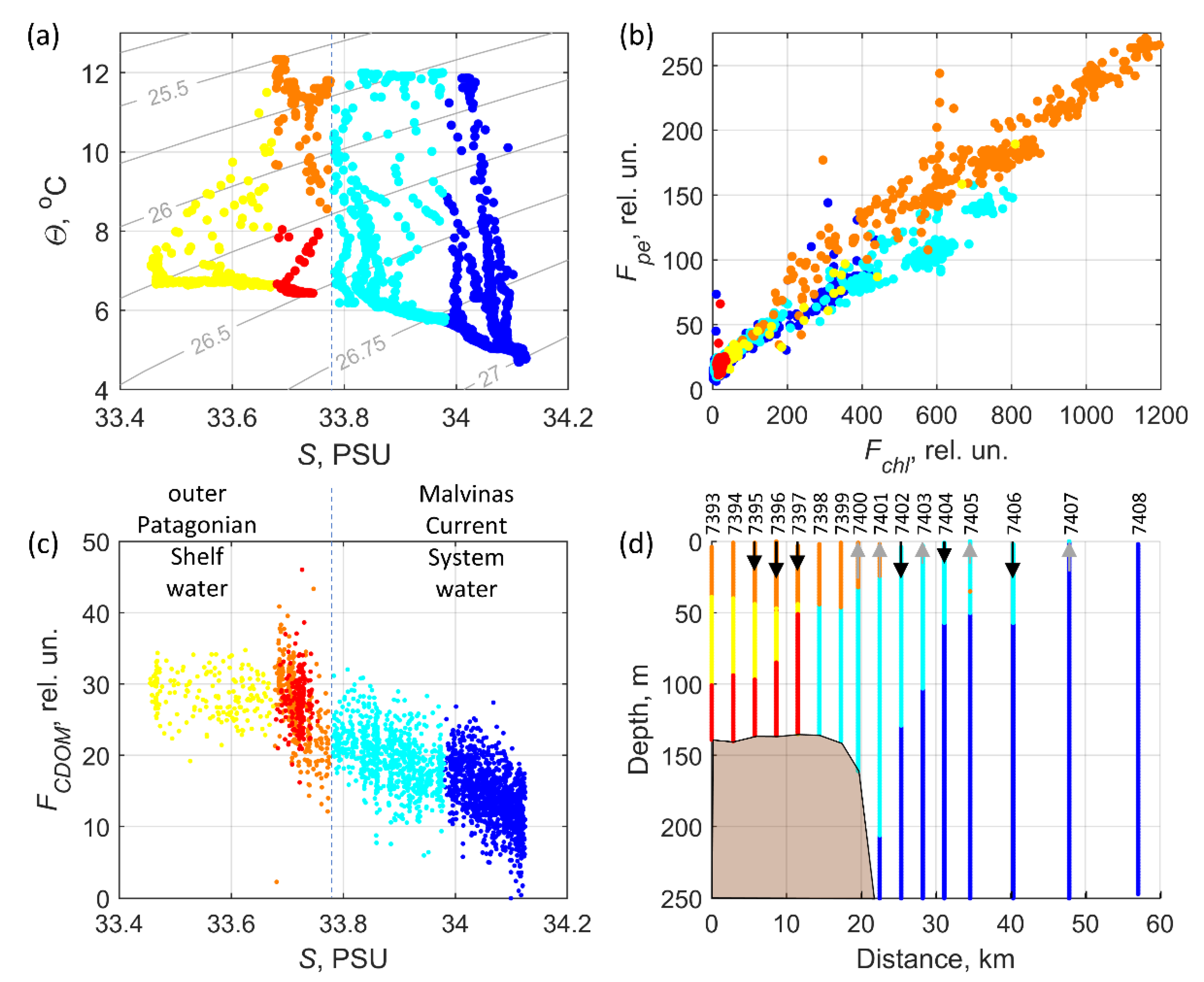
| ID, Region, Water Mass Description | Color | Criteria | Characteristics |
|---|---|---|---|
| Y, Patagonian Shelf, intrusion from the distant part of the shelf | Yellow | S < 33.675 | No correlation between salinity and CDOM fluorescence, relatively low salinity and high FCDOM values |
| R, Patagonian Shelf, upwelled bottom waters of the outer shelf | Red | S ≥ 33.675 & S < 33.78 & Depth ≤ 50 m | Low anticorrelation between salinity and CDOM fluorescence, relatively high FCDOM and Turb values |
| O, Patagonian Shelf, high bio-productive water of the outer shelf | Orange | S ≥ 33.675 & S < 33.78 & Depth > 50 m | High anticorrelation between salinity and CDOM fluorescence, specific phycoerythrin/chl-a fluorescence relationship, relatively high FCDOM and Fchl values |
| C, Malvinas Current System, mainly in the inshore branch of the MC over continental slope | Cyan | S ≥ 33.78 & S < 33.95 | Low anticorrelation between salinity and CDOM fluorescence |
| B, Malvinas Current System, mainly between inshore and offshore branches of the MC | Blue | S ≥ 33.95 | Low anticorrelation between salinity and CDOM fluorescence, relatively low FCDOM values and high salinity |
| Stations | 7393 | 7395 | 7397 | 7400 | 7401 | 7402 | 7404 | 7406 |
|---|---|---|---|---|---|---|---|---|
| Dinoflagellates | 12.4 | 36.3 | 30.9 | 16.7 | 22.2 | 22.7 | 35.8 | 50.0 |
| Diatoms | 10.7 | 6.7 | 22.2 | 2.8 | 16.7 | 0.0 | 9.4 | 12.5 |
| Pyramimonads | 77.0 | 57.0 | 46.9 | 80.6 | 61.1 | 77.3 | 49.1 | 37.5 |
| Dictyocha fibula | 0.0 | 0.0 | 0.0 | 0.0 | 0.0 | 0.0 | 1.9 | 0.0 |
| Pterosperma cf. polygonum | 0.0 | 0.0 | 0.0 | 0.0 | 0.0 | 0.0 | 3.8 | 0.0 |
| Station | Bottom Depth, m | UML Depth, m (Figure 4) | Euphotic Depth, m (Figure 7) | Up or Down Vert. Dir. * (Figure 4) | Region, (Figure 1 and Figure 2) | Water Mass, (Figure 6, Table 2) | Phytoplankton Group ** (0–50 m), (Figure 9) | Zooplankton Group (0–200 m), (Figure 11) | Birds’ Density, ind/h (Figure 12) |
|---|---|---|---|---|---|---|---|---|---|
| 7393 | 137 | 38 | 29 | PS | R, Y, O | Am | A | ||
| 7394 | 140 | 39 | 28 | PS | R, Y, O | ||||
| 7395 | 136 | 42 | 29 | D | PS | R, Y, O | Am | A | 72.6 |
| 7396 | 134 | 45 | 31 | D | PS | R, Y, O | |||
| 7397 | 134 | 41 | 31 | D | PS | R, O | Am | A | |
| 7398 | 139 | 37 | 37 | PS, MCi | C, O | A | |||
| 7399 | 139 | 37 | 38 | PS, Mci | C, O | ||||
| 7400 | 155 | 30 | 42 | U | Pse, Mci | C, O | Bm | B | |
| 7401 | 293 | 24 | 40 | U | Pse, Mci | B, C, O | Bm | B | 10.3 |
| 7402 | 365 | 45 | 34 | D | Mci | B, C | no cluster | B | |
| 7403 | 462 | 35 | 41 | U | Mci | B, C | |||
| 7404 | 631 | 44 | 40 | D | Mci | B, C | Cm | no cluster | |
| 7405 | 742 | 35 | U | Mci | B, C | ||||
| 7406 | 790 | 53 | D | Mci | B | Cm | C | ||
| 7407 | 853 | 25 | U | ZB | B | ||||
| 7408 | 942 | 39 | ZB | B | C | ||||
| - | >1000 | ? | ZB & MCo | - | 19.0 |
Publisher’s Note: MDPI stays neutral with regard to jurisdictional claims in published maps and institutional affiliations. |
© 2022 by the authors. Licensee MDPI, Basel, Switzerland. This article is an open access article distributed under the terms and conditions of the Creative Commons Attribution (CC BY) license (https://creativecommons.org/licenses/by/4.0/).
Share and Cite
Salyuk, P.A.; Mosharov, S.A.; Frey, D.I.; Kasyan, V.V.; Ponomarev, V.I.; Kalinina, O.Y.; Morozov, E.G.; Latushkin, A.A.; Sapozhnikov, P.V.; Ostroumova, S.A.; et al. Physical and Biological Features of the Waters in the Outer Patagonian Shelf and the Malvinas Current. Water 2022, 14, 3879. https://doi.org/10.3390/w14233879
Salyuk PA, Mosharov SA, Frey DI, Kasyan VV, Ponomarev VI, Kalinina OY, Morozov EG, Latushkin AA, Sapozhnikov PV, Ostroumova SA, et al. Physical and Biological Features of the Waters in the Outer Patagonian Shelf and the Malvinas Current. Water. 2022; 14(23):3879. https://doi.org/10.3390/w14233879
Chicago/Turabian StyleSalyuk, Pavel A., Sergey A. Mosharov, Dmitry I. Frey, Valentina V. Kasyan, Vladimir I. Ponomarev, Olga Yu. Kalinina, Eugene G. Morozov, Alexander A. Latushkin, Philipp V. Sapozhnikov, Sofia A. Ostroumova, and et al. 2022. "Physical and Biological Features of the Waters in the Outer Patagonian Shelf and the Malvinas Current" Water 14, no. 23: 3879. https://doi.org/10.3390/w14233879