
Variability of Annual and Monthly Streamflow Droughts over the Southeastern United States

1
Northern Gulf Institute, Mississippi State University, 2 Research Blvd, Starkville, MS 39759, USA
2
Department of Geosciences, Mississippi State University, 200A Hilbun Hall, Mississippi State, MS 39762, USA
*
Author to whom correspondence should be addressed.
Water 2022, 14(23), 3848; https://doi.org/10.3390/w14233848
Submission received: 7 November 2022
/
Revised: 21 November 2022
/
Accepted: 24 November 2022
/
Published: 26 November 2022
(This article belongs to the Special Issue Assessing Hydrological Drought in a Climate Change: Methods and Measures)
Abstract
:Understanding the patterns of streamflow drought frequency and intensity is critical in defining potential environmental and societal impacts on processes associated with surface water resources; however, analysis of these processes is often limited to the availability of data. The objective of this study is to quantify the annual and monthly variability of low flow river conditions over the Southeastern United States (US) using National Water Model (NWM) retrospective simulations (v2.1), which provide streamflow estimates at a high spatial density. The data were used to calculate sums of outflow deficit volumes at annual and monthly scales, from which the autocorrelation functions (ACF), partial autocorrelation functions (PACF) and the Hurst exponent (H) were calculated to quantify low flow patterns. The ACF/PACF approach is used for examining the seasonal and multiannual variation of extreme events, while the Hurst exponent in turn allows for classification of “process memory”, distinguishing multi-seasonal processes from white noise processes. The results showed diverse spatial and temporal patterns of low flow occurrence across the Southeast US study area, with some locations indicating a strong seasonal dependence. These locations are characterized by a longer temporal cycle, whereby low flows were arranged in series of several to dozens of years, after which they did not occur for a period of similar length. In these rivers, H was in the range 0.8 (+/−0.15), which implies a stronger relation with groundwater during dry periods. In other river segments within the study region the probability of low flows appeared random, determined by H oscillating around the values for white noise (0.5 +/−0.15). The initial assessment of spatial clusters of the low flow parameters suggests no strict relationships, although a link to geologic characteristics and aquifer depth was noticed. At monthly scales, low flow occurrence followed precipitation patterns, with streamflow droughts first occurring in the Carolinas and along the Gulf Coast around May and then progressing upstream, reaching maxima around October for central parts of Mississippi, Alabama and Georgia. The relations for both annual and monthly scales are better represented with PACF, for which statistically significant lags were found in around 75% of stream nodes, while ACF explains on average only 20% of cases, indicating that streamflow droughts in the region occur in regular patterns (e.g., seasonal). This repeatability is of greater importance to defining patterns of extreme hydrologic events than the occurrence of high magnitude random events. The results of the research provide useful information about the spatial and temporal patterns of low flow occurrence across the Southeast US, and verify that the NWM retrospective data are able to differentiate the time processes for the occurrence of low flows.
1. Introduction
Due to increasing population stress on existing water resources and water quality, as well as uncertainty associated with current and future climate variability, understanding drought formation and evolution processes has become extremely important. As a result, the ability to accurately model and predict droughts is a critical step not only for maintaining the natural environment, but also for ensuring the needs for human water resources. The growing importance of droughts, especially in the light of the latest research showing the intensification of this phenomenon in the coming years [1,2,3,4,5,6]; Wang et al. [7], raises questions about forecast accuracy, and more importantly, the scale at which accurate drought predictions can be produced. The first, and perhaps the most important, problem in any forecast or analysis process for any natural phenomenon is data availability. For investigation of hydrological processes, river flow data are usually collected by governmental institutions, such as the United States (US) Geological Survey (USGS). Although the data collected by these institutions provide accurate and reliable observational datasets, the length of these datasets is related to the history and ability to perform continuous measurements at each gauge. This leads to limitations in the possibilities of spatial analysis of hydrological phenomena in areas with sparse and/or incomplete gauge information, and further hinders the development of modeling frameworks that allow for realistic simulations in places for which real data are not available.
Large-scale hydrologic models, in order to maintain computational feasibility and physical representativeness, must use spatial and temporal resolutions representative of the larger model domain; therefore, they often cannot accurately reflect local conditions related to geology, groundwater, heat fluxes, or evapotranspiration, which are important from the drought perspective [8,9,10,11,12,13]. On the other hand, complexity of local conditions makes it difficult to generate and maintain accurate local-scale models, especially when these conditions themselves evolve over space and time; therefore, some level of generalization must be introduced to produce a baseline simulation.
In 2016 the US National Oceanic and Atmospheric Administration (NOAA) contributed to the improvement of the accuracy and spatial coverage of data related to the observation, assessment, and prediction of hydrological extreme events over the continental United States (CONUS) by developing a hydrologic modelling framework called the National Water Model (NWM). The NWM is based on the Weather Research and Forecasting–Hydrological Modeling System (WRF-Hydro), and provides operational simulations of land surface and hydrologic conditions at a variety of time scales (e.g., short, medium, and long range). In addition to the operational version of the model, each major version of the simulation framework is used to produce a historical (also known as, retrospective) simulation for research and analysis purposes. These simulations are forced with the North American Land Data Assimilation (NLDAS) data sets for versions 1.2 and 2.0 and Office of Water Prediction Analysis of Record for Calibration (AORC) data for version 2.1. Thanks to this approach, the NWM has become the substrate for the large-scale distributed simulation of hydrological conditions across the US. Streamflow simulations are dependent on multiple surface and hydrological parameters, of which precipitation and snowmelt play major roles. The main limitations of the NWM include the inability to reproduce reservoir management flows [14,15], especially in previous versions of the model (i.e., v1.2 and v2.0) although the newer operational version of the model (v2.1) includes new reservoir treatment that leverages River Forecast Center (RFC), USGS and U.S. Army Corps of Engineers (USACE) data feeds. While this improves the model response for river segments located below reservoir, some artifacts might still exist [16]. The ability to simulate hydrological conditions at 2.7 million stream locations nationwide means not only better forecasts of water resources, but also improved safety and stability of communities, industry, and protection of life and property [17]. Additionally, retrospective simulation datasets provide continuous surface and hydrologic records for all computational nodes covered by the operational version of the NWM, which in turn allows for analysis of historical hydrological conditions without restrictions related to locations of river observation sites.
A primary motivation for the development of the NWM was the improvement of flood prediction information and dissemination, which are the costliest and deadliest type of natural disasters in the United States [18]. This approach contributed to an improved mathematical representation of the upper range of flows over a large spatial extent; however, due to the increasing importance of droughts in recent years [19], the ability to apply the NWM to drought assessment has become an important topic [20,21]. This is especially true given that due to climate change water resources are more likely to behave in a non-stationary way [22], requiring the use of comprehensive physical models such as the NWM to provide meaningful predictions of hydrologic drought conditions. There is some evidence of NWM performance being linked to river basin size [23,24], or location, with streams underperforming in semiarid environments [25] or in rivers sensitive to snowmelt runoff [26]. As a result, the NWM has been shown to perform better in streams with a precipitation forced regime [21], and in general the NWM is able to capture major droughts [27] and general streamflow patterns in humid regions such as the Southeastern United States [20].
The aim of this work is to assess the variability of streamflow droughts at annual and monthly scales over the Southeastern United States, based on NWM retrospective v2.1 data, to quantify the spatial and temporal patterns of regional hydrologic drought. The study area is characterized by abundant water resources affected by stress due to industrial and agricultural water withdrawals. This stress is further exacerbated by advancing climate change resulting in changes of water resources and increasing drought risk [28,29,30,31]. The four main research questions posed in this paper are as follows: (i) can NWM retrospective data represent low flow occurrence patterns at different time scales, and differentiate regional dependencies, (ii) what are the patterns of hydrologic drought occurrence in terms of annual and monthly variability, (iii) what are the spatial patterns and associated physical drivers of streamflow drought generation and progression, and (iv) are these patterns reflected in the NWM retrospective data, such that machine learning-based occurrence models can be developed to predict future development of streamflow droughts? Autocorrelation and partial autocorrelation were used as the primary analysis tools within this study, providing information about statistically significant periods of streamflow droughts, as well as quantifying the significance of streamflow drought occurring as an extreme event, more or less randomly, versus reoccurrence in periods related to seasonality. The difference between the two occurrence patterns was further measured with the Hurst exponent statistic, which allows for assessment of so called “process memory”. The analysis of variability in the hydrologic data will allow for the recognition of fluctuations in low flow events over time. This, in turn, will allow for the construction of models of the phenomenon, based on time dependencies, for example using machine learning approaches. Additionally analysis will provide critical information regarding not only the utility of the NWM retrospective data to define and represent low flow conditions and associated characteristics, but will allow for the generation of a baseline dataset that can be used for subsequent investigations of streamflow drought patterns and processes across the Southeast US for water resource assessments.
2. Study Area
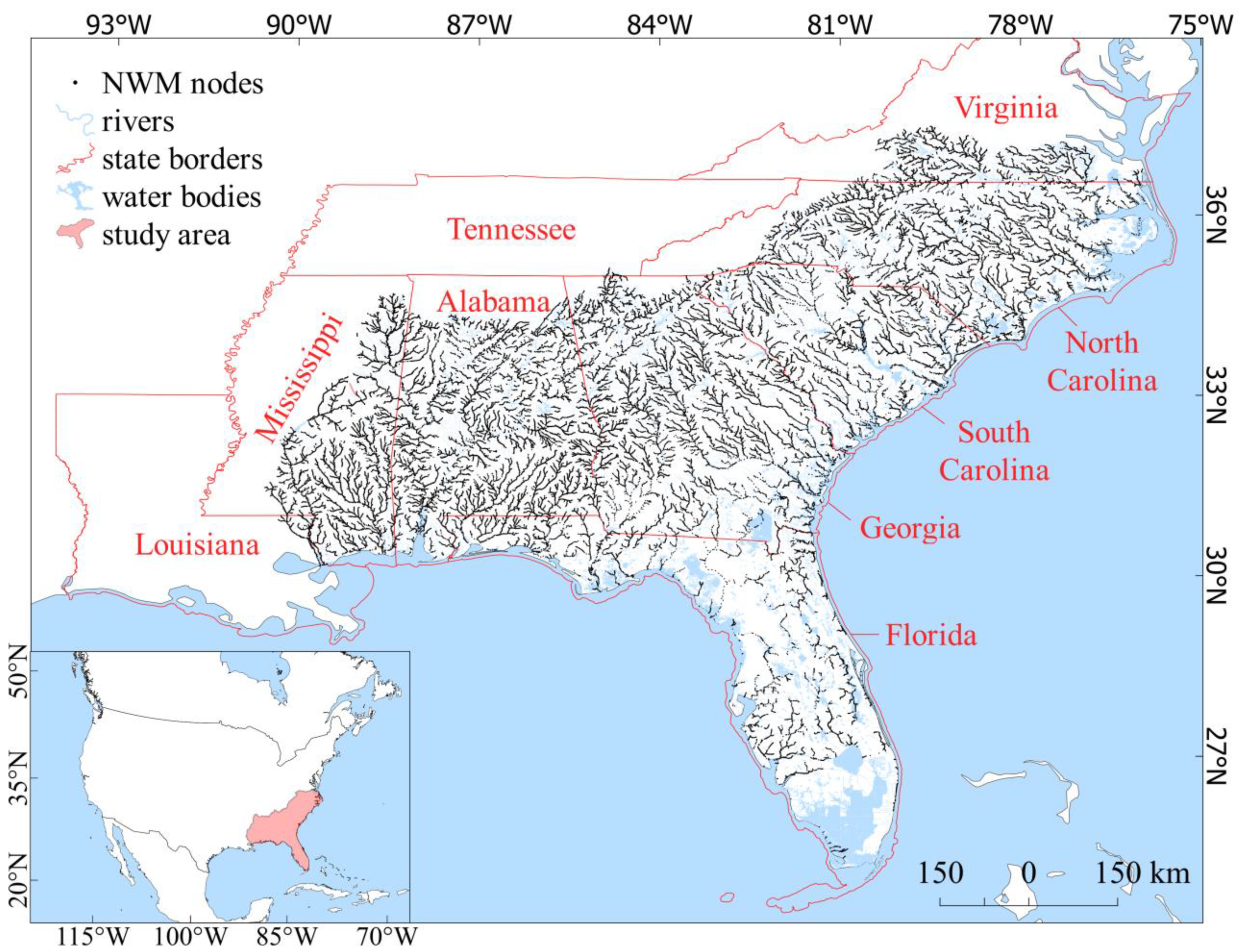
The study area constitutes the southeastern part of the US, specifically identified in a hydrologic context as USGS Region 3: South Atlantic-Gulf Region (Figure 1). This region, which includes all rivers flowing to the Atlantic Ocean and the Gulf of Mexico between the James River catchment in Virginia and the Lower Mississippi River in Mississippi, comprises a total area of ~724,000 km2. The area incorporates a diverse array of natural landscapes, with variable land use/cover, vegetation, meteorological, and geological characteristics that lead to a range of hydrologic conditions. The Coastal Plain, a major part of the region that represents around 60% of the total area, is composed mainly of soft unconsolidated sands, gravels, and clays or consolidated and semi-consolidated limestone. The northern regions within the Appalachian highlands contain mainly hard, consolidated rocks, indurated and metamorphosed sedimentary rocks, and crystallin igneous rocks. Groundwater is associated mainly with Cretaceous and Quaternary deltaic sand and gravel deposits, with daily groundwater discharge of around 0.3 km3 that moves seaward in a pattern reflective of the general layout of the regional river networks [32]. Elevation varies between −25–1589 m.a.s.l. over the area, and average stream density is 0.24 km/km2 (total river length is ~175,000 km). Stream density has a high regional variability, with a denser network in the northern and northeastern areas and a sparse river network in the south. Approximately 60% of streamflow is contributed by baseflow and 40% by direct runoff [33].
The climate over the majority of the area is subtropical, with hot and humid summers. Mean annual temperature is between 14 °C–25 °C, depending on the region [25], and annual precipitation varies between 1000 to 2000 mm/year. The relation between water resources and climate variability is strong [34,35], and longer-term changes in precipitation, evaporation, and runoff are caused mainly by the El Niño-Southern Oscillation (ENSO), which affects terrestrial water storage and associated anomalies as well as streamflow discharges [35,36,37,38]. Occurrence of La Niña is connected with higher maximal temperatures and lower precipitation, mainly noticeable in June [29], with some evidence showing varying links to dry winters with La Niña in the past, that now depends purely on internal atmospheric variability [31,39]. Decreasing streamflow trends are observed during water-year and spring-summer periods, with strong evidence of abrupt step changes being of greater importance than gradual changes over past years [40]. Constant decrease in streamflow of rivers over the study area is linked to increasing sea surface temperatures [38,41]. Due to the specific environmental conditions of the region, increasing population, growing agriculture needs as well as changes in local climate patterns, Alabama, Mississippi and Florida are identified as regions facing water supply shortages in the future [42]. Further evidence also shows that the entire region faces a substantial drought threat both now and in the future, mainly due to increasing water demands, limited storage capacity, and agricultural dependance on precipitation [43,44,45], as local water supply regulations were often developed during wetter periods in the region [46].
3. Data and Methods
3.1. Hydrometeorological Data
Streamflow information for this study comes from the NWM retrospective v2.1 dataset, which contains 338,037 unique retrospective stream nodes (hereafter referred to as nodes) with a period of record of February 1979–December 2020. After data quality evaluation a decision was made to include only nodes of Strahler order 3 and higher, since lower orders contained over 80% zero values, which from the perspective of drought analysis introduces the risk of non-representative threshold levels and drought event statistics. This decision also relates to a general limitation of the NWM, such that the model underperforms in lower order streams [23,24]. Additional criteria of no more than 5% of zero or null data were introduced to avoid computational errors, and an additional 1198 nodes were characterized by almost unchanging minimum flow values, which led to the defined low flow threshold (see below for method details) being the same value as the minimum flow. These nodes were excluded from the study, leading to the inclusion of 60,750 nodes with hourly mean streamflow values, which were converted to daily mean flow values representing 00–00 UTC. The final dataset constituted daily flows for a period from 1 February 1979–31 December 2020, which equates to 2,551,500 stream years.
Precipitation data, which was used for analysis of low flow processes, was obtained from the U.S. Federal Government Climate Resilience Toolkit [47] for monthly and annual scales.
3.2. Low Flow Conditions Definition
In this study, low flow definition is based on the widely adopted threshold level method (TLM; [48]), whereby stream discharge is considered low flow if it is equal to or lower than a defined threshold level. There are many ways of calculating a threshold; however, this study adopts an objective breakpoint method to define unique threshold levels at each node. In this approach, the lower part of the flow duration curve (FDC) is considered as a series with a breakpoint that serves as the indicator of the moment of change from atmospheric supply to groundwater supply, which constitutes a natural marker for the beginning of low flow conditions. This method is described in detail by Raczynski and Dyer [49]. To accurately measure the seasonal and annual outflow deficits, no pooling method and no additional minimal time criteria were applied. In this study the term low flow refers to discharge values identified as lower or equal to a threshold discharge level, while low flow event/conditions are considered the same as streamflow drought—a series of low flows that occur over some period that lead to formation of hydrologic drought.
3.3. Statistical Analysis
A basic parameter used in this study is a low flow volume (V) which is calculated as a difference between the defined streamflow threshold and the flow hydrograph during drought episode:
where: V—volume (m3), Qt—threshold flow (m3 s−1), and Q—outflow (m3 s−1).
To describe changes in episodes occurrence, autocorrelation functions (ACF) were calculated for event volumes aggregated to monthly and annual scales. Autocorrelation allows for examination of seasonal or multi-annual variations in low flow conditions by estimating the degree of correlation between element with element shifted by k [50], where the length of this shift (also referred to as lag) may vary:
where s0 is variance of the time series at t and sk is covariance at k lag:
For this study, a time series constitutes of low flow volumes in a single node aggregated to monthly or annual scale.
In order to assess the possibility of applying data from NWM to occurrence models based on machine learning techniques, the number of lags needed to obtain statistically significant result should be estimated. Based on the information about the significance of the lags (q) of the autocorrelation functions, the usefulness of potential seasonal models can be estimated. The model based on the seasonality resulting from the autocorrelation relationship is the moving average (MA(q)) model, which is expressed by the number of statistically significant correlations of lags in ACF. For example, the MA(7) model means that the modeled dependence has statistically significant relationships up to the 7th lag (seven periods back—depending on the resolution of the tested series, e.g., months or years). In addition to ACF, partial autocorrelation functions (PACF) were calcualted to introduce the control of all lags. PACF explains partial correlation between the series and lags of itself. Significance of PACF lags (p) provides valuable information on potential lag steps in seasonal modeling using autoregressive models (AR(p)), as significant PACF lags (p) correspond to lags in AR(p) models on the same basis as ACF lags (q) are used for the MA(q) models [51,52]. Therefore, estimating whether and at which lag there are statistically significant relationships in ACF and PACF distributions constitute the basis for assessing whether the studied relationships can, at a later stage, be modeled using machine learning techniques, using the AR and/or MA seasonality models.
Summability or non-summability of the autocorrelation function is an indicator of the process memory length, which describes the tendency for grouping of natural extreme events into sequences. So-called “process memory” was first observed in hydrologic data by Hurst [53], which led to the development of the Hurst exponent (H) that describes the process memory length within a hydrologic data series. The detailed methodology for determining the value of the exponent was described by Koutsoyiannis [54]. Values of H close to 0.5 reflect white noise processes, where consecutive values are random, while H values closer to 1 reflect long process memory, understood as a tendency for similar events to group in longer sequences (large values are followed by large values, and vice versa). Although in natural processes the range of H is usually 0.5–1 [54], it is possible for H to range from 0–0.5, where values H < 0.5 means an anti-persistent series where high and low values appear alternately.
To classify spatial relations between groups of nodes with similar process memory, an unsupervised machine learning algorithm of K-means clustering was applied. The algorithm is used to group similar data into clusters by minimizing the objective function J(z,A) with updating cluster centers [55]:
where c is number of clusters, xi is the data point, ak is cluster center, and zik is a binary variable that indicates if the data point is considered within the cluster.
All statistics were performed for two-tailed α = 0.05.
4. Results and Discussion
4.1. Annual Distribution
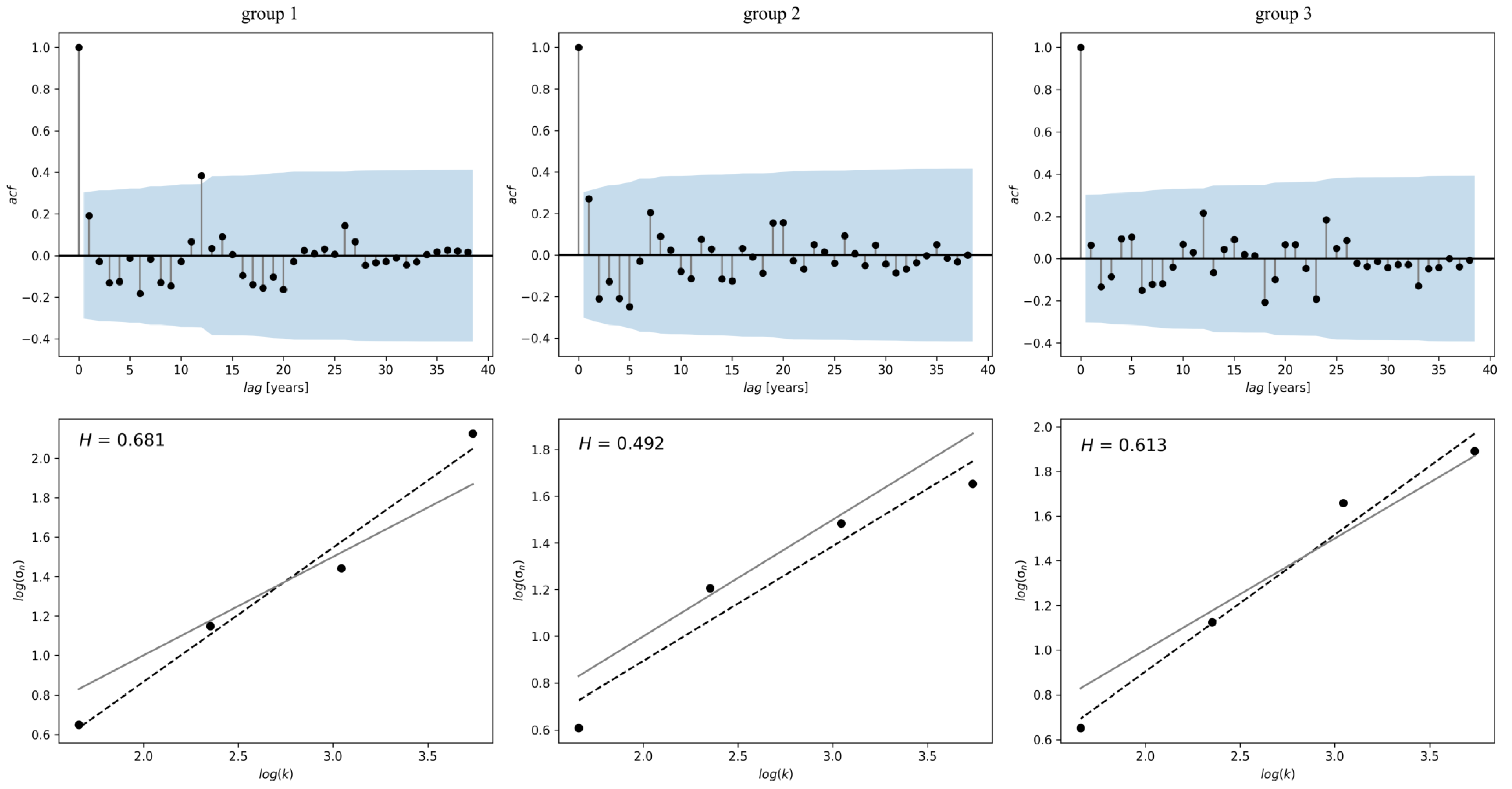
To determine annual patterns of streamflow droughts, the daily water outflow deficiencies (volumes) were aggregated to the annual scale. It was expected that at least two different ACF shapes would be obtained as indicated in other works [56,57], and analysis confirmed that these patterns are present in the dataset. In the first case the pattern of low flow occurrence is close to random and the majority of the ACFs are statistically insignificant, with autocorrelation values shifting every year or so. H for these rivers is close to white noise with a mean of 0.59 (Figure 2), and 26% of the analyzed nodes were classified in this group. These patterns are usually described as related to meteorological conditions, and are easy to predict [10,58]. An example of this type of process is presented in Figure 2, where low flows occurred in around half of the 42-year study period (average of 18.5 years with low flow and 23.5 without low flow). On average there were 15 shifts between years with and without low flows, and episodes occur in two to three consecutive years and then disappear for a similar period.
The second, and at the same time the largest group (65% of nodes), were rivers with low flows occurring in about 6–7 year intervals with 1–2 year breaks in occurrence (Figure 2). Similar to the first group, an average of 14 shifts were observed during the study period. In total, low flows occurred during 32 of the 42 years in the study period. H for this group is 0.70 and ACFs show higher repeatability, indicating that groundwater is of greater importance in these types of rivers, especially when multi-annual streamflow drought occurrence is present [11,59,60].
There is also a third group that constituted less than 9% of the analyzed nodes, and included rivers where low flow occurred almost annually (mean of 40 years with low flow over the study period; Figure 2). The average H is closer to representing white noise than for the second group, having a mean value of 0.63, which is most likely due to the high irregularity of shifts in occurrence along with the relatively short period (on average one year).
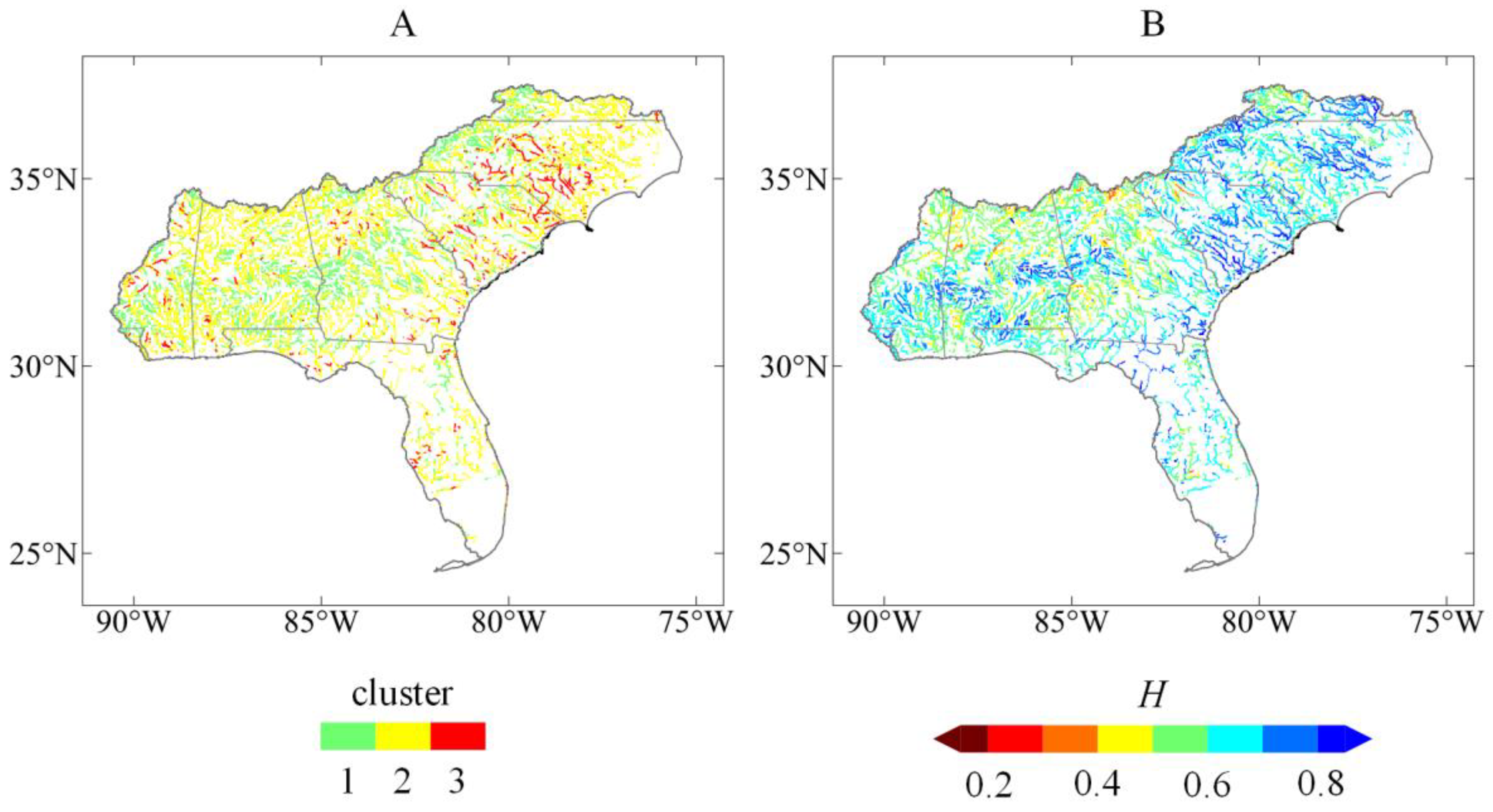
Analysis of the spatial distribution of the clusters showed no statistically significant correlation between the type of low flow occurrence and stream order, and in fact there are some rivers along which the cluster changes along the stream. Most nodes with low flow patterns that fall within the third group are located in North Carolina, especially in the Cape Fear and Pee Dee River systems, as well as in the upper Pearl River watershed in Mississippi. The lowest frequency of low flow occurs in central parts of Mississippi, Alabama and Georgia, below the Appalachian piedmont, as well as in northern parts of the Carolinas in upstream river sections (Figure 3 and Figure 4). The former relation might be explained by groundwater inflow to rivers located at the base of the Appalachian Mountains, while deeply allocated aquifers in the piedmont region of the Carolinas may explain the high magnitude of low flows in that area.
High values of H are observed in both North and South Carolina, where over 80% of nodes are characterized by H higher than 0.6 and around half of nodes with H higher than 0.7. This suggests that longer process memory occurs in this region; however, defined ACF clusters do not accurately reflect spatial relations for part of study area. While Virginia and the Carolinas show relatively high values of H, suggesting strong seasonality, ACF clustering finds most of these rivers belong to the Cluster 1 (Figure 3). Additionally, statistically significant decreasing trends are observed in the Carolinas, meaning low flows are in general becoming more severe [61,62]. Multiyear droughts with high magnitudes were also identified in this region [62], which is confirmed by high H values found in this study. High magnitude, recurring streamflow droughts in the Carolinas with increasing trends are associated with decreased precipitation and increased potential evapotranspiration, especially in the July-September warm-season period, as the changes correspond to variations in meteorological factors [59,63]. This dependence is further intensified by long recovery times after dry conditions are gone [64] and agricultural practices such as irrigation that affect negatively water supplies in the region [65].
High values of H (>0.7) are also observed for central and southern parts of Alabama and Georgia (Figure 3B), where ACFs alter every 2–3 years. This is in contrast to clustering results, as H values suggest relatively easy to predict processes taking place in this region, while the cluster average was close to white noise. However, evidence of seasonality of low flows is seen from central Mississippi to north central Georgia, where increases in H are related to intervals of ACF Cluster 2. This might be due to high repeatability of 2–3-year patterns in these nodes while ACF functions were variable, resulting in a shape reminiscent of random processes. This relation is likely affected to some degree by ENSO, as during these conditions over the southeast US intense groundwater withdrawals for irrigation are observed that act to decrease baseflow and lower low flows [66]. Decreasing values of low flows in this region, however, might be also linked to additional human-induced influences [67], related mainly to land-use, population growth, and agriculture [66,68,69].
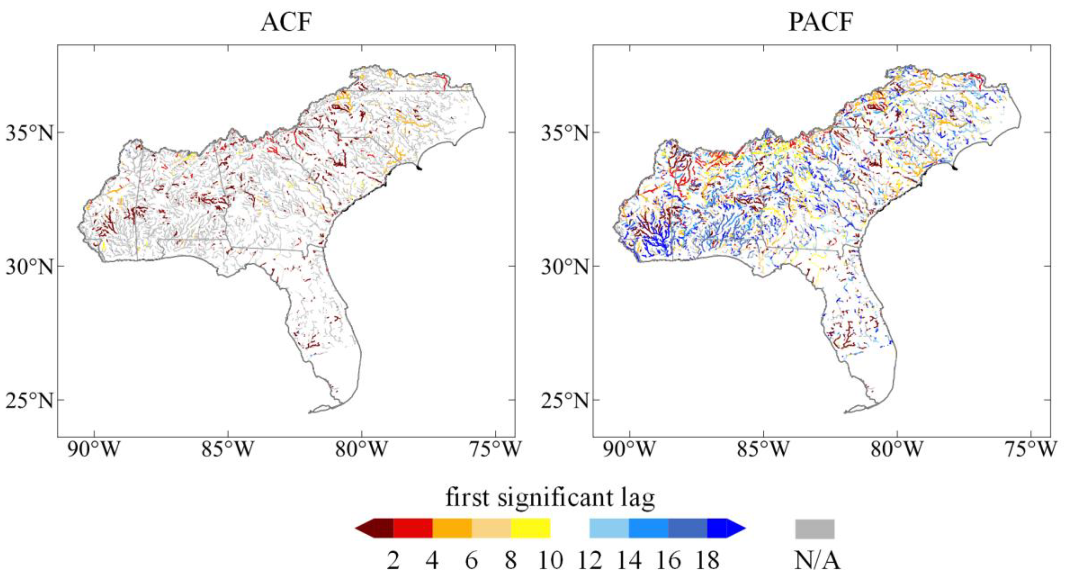
For less than half of the studied nodes in Alabama and Georgia, first, second and third lags were statistically significant. This relation is visible for other regions in the study area as well, where only a fraction of nodes with high H values yield significant autocorrelations. In total, 83.8% of all nodes do not have any significant lag (of the first 20 lags) and only 7.9% have the first lag significant (Table 1). These results indicate that there is no constant, univariate process that could be quantified by averaged seasonal models as residuals are not linearly dependent on current and past values. PACF distribution (Figure 4) in most nodes contains some statistically significant lags, and from all studied nodes, around 27% do not contain statistically significant p lags (Table 1). This dependence suggests that models based on seasonal repeatability defined by the autoregressive component (AR(p)) might reflect the actual changes in the annual occurrence of low flows better than moving average (MA(q)) models.
4.2. Monthly Distribution
Although annual distributions of low flow occurrences show some spatial dependencies, the monthly distribution provides a better understanding of the processes. In general, the distribution of monthly streamflow droughts follows precipitation patterns, which was also confirmed in other studies [5,63]. The relations are strongest along the Atlantic coast, where sandy soils lead to relatively rapid hydrologic response of river levels to rainfall. January low flow frequency is at or near zero in 64% of nodes over the study period, with mainly low magnitude events in Florida and southern Georgia; however, evidence suggests some relation to precipitation is also present in Virginia. In subsequent months, low flows continue to disappear in the majority of the study area except Florida, where winter precipitation is on average around 40 mm/month and there is a clear, strong relation with streamflow drought characteristics and precipitation through April, measured by the Spearman rank correlation (Figure 5). This pattern matches general climatic features, with subtropical regions north of Florida having a wet winter, while Florida has a relatively drier winter as it reflects a tropical climate.
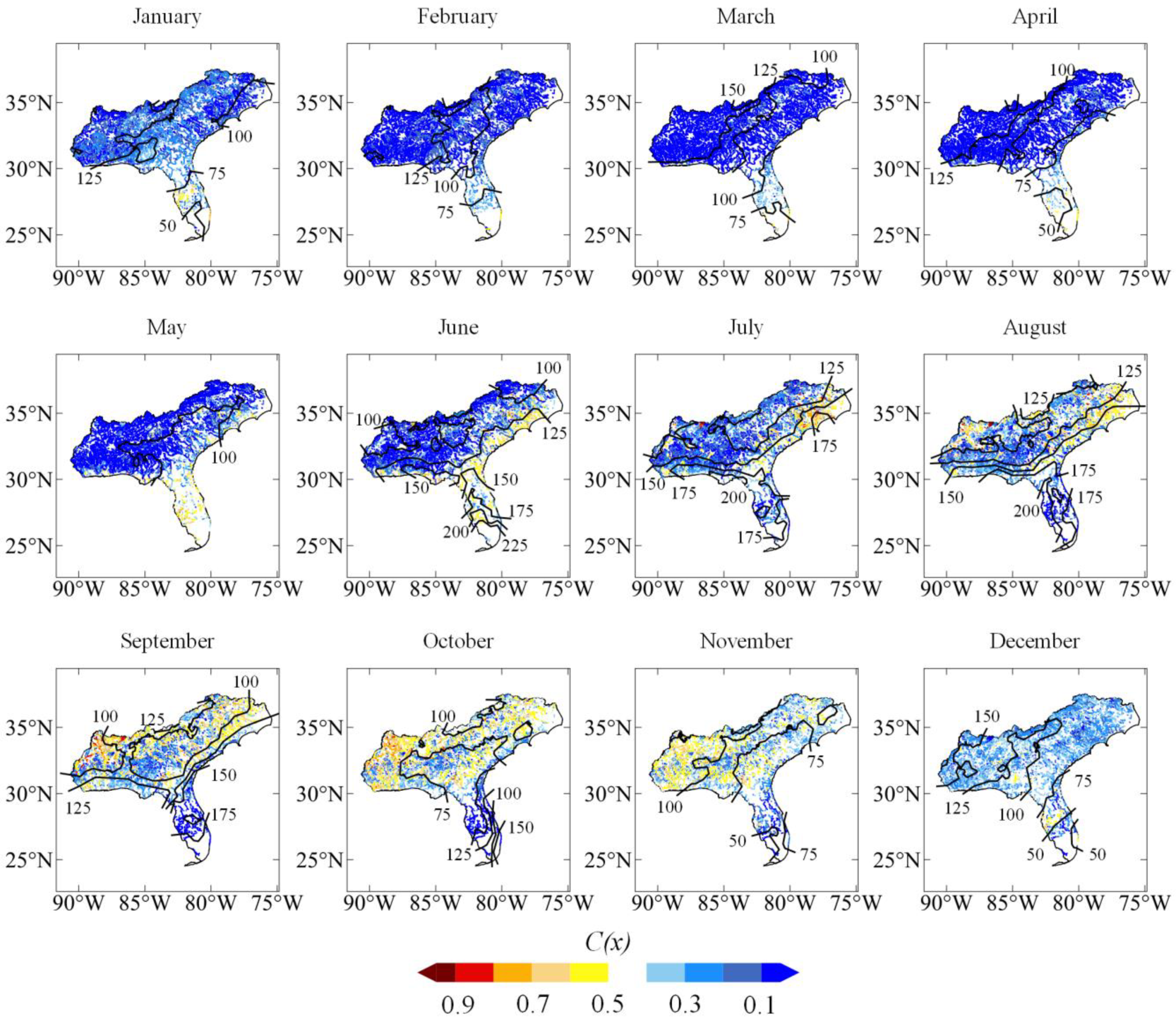
During spring (April–June) there is also increased risk of flash droughts in northern and western Florida as well as south Georgia, which was observed by [70]. Starting from May the precipitation patterns begin to change due to the difference in climate patterns between Florida and the Gulf Coast and areas to the north, when sums of precipitation increase over Florida (tropical climate) and decrease through the central and northern study area (sub-tropical climate, Figure 6). In May and June low flows occur mainly over Florida and southern Georgia, while over the following months low flows continue to develop from the Gulf Coast toward central and western parts of the study region (Figure 6). During this time the relation of low flows to precipitation weakens (Figure 5), likely due to increased potential evaporation [59]. At the same time Florida’s low flows disappear due to increased precipitation. This spatial direction is consistent with patterns in development of flash droughts found by Chen et al. [70]. In general, droughts related to climatic forcings are regionally specific, with a clear relation between increases in drought with precipitation decreases and potential evaporation increases, especially for north Florida, North Carolina, and Virginia [28,71].
The highest periodicity of low flows changes by region, with the most intense low flows occurring in July in North Carolina (also annual maxima), in September and October in Mississippi and northern Alabama, and November in the piedmont region (Figure 6). The region of north-central Alabama was also found to be most prone to drought persistence within the study region [72]. The summer period (July–October) is also characterized by high periodicity, reaching 25–30 repeats with low flow each month over the study period, especially in the central and northern parts of the study region. This dependence is opposite to the precipitation distribution, where the Carolinas are characterized by high monthly mean precipitation reaching 175 mm in Coast area, while at the same time the periodicity is highest (Figure 6), emphasizing the role of lowering groundwater levels due to pumping presented by [59]. During late winter and spring a substantial number of nodes had no streamflow droughts during the entire study period, with the total percentage of nodes showing no low flows being 13% in February, 32% in March, 34% in April, and 16% in May.
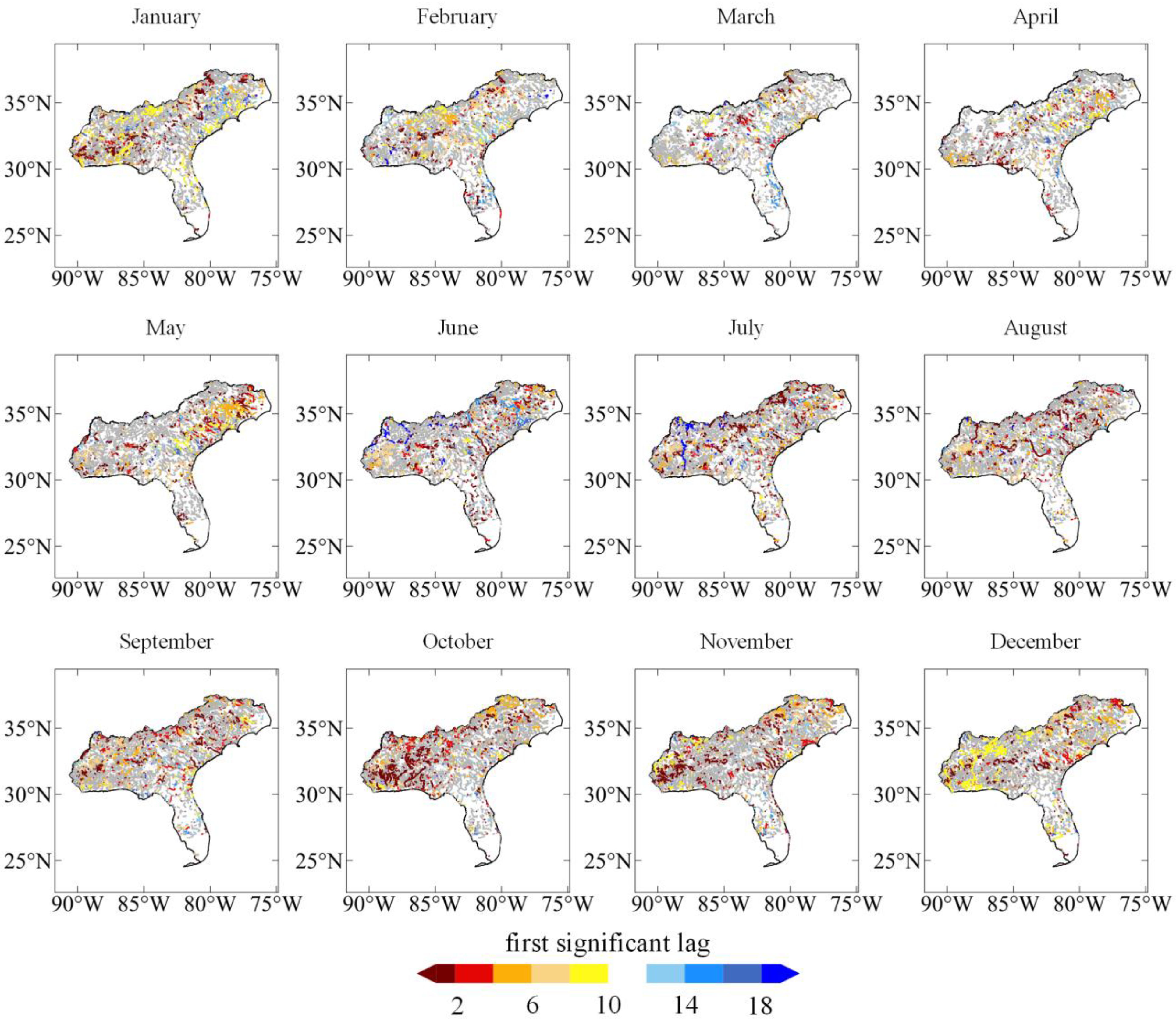
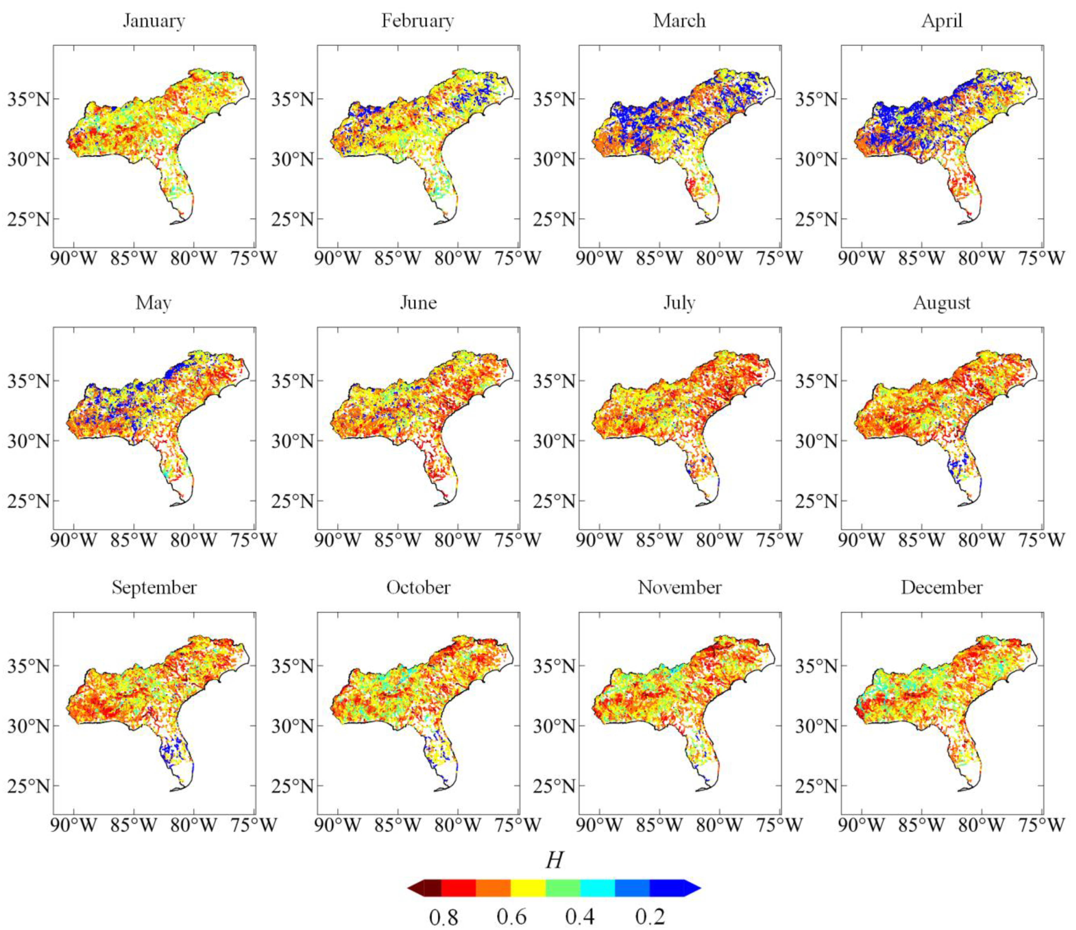
Similar to annual observations, PACFs generally provide more information than ACFs. The latter on average were statistically significant for around 20% of nodes, with mostly insignificant functions in all 20 lags for April (85.3%) and the lowest values over the winter period (December–February, on average 79%). In most cases, significant ACF lags were related to lag 1 or 12, which follows seasonal and annual patterns. When considering PACFs, on average 60% of nodes contain statistically significant lags, with the highest number for November (79%) and lowest for March (33%). In general, ACFs and PACFs provide the same pattern as described before, with the lowest explanatory power during March and April due to lowest number of drought episodes, and then increasing in lag significance from May over the Carolinas and Gulf Coast before progressing inland. Around June and July the highest concentration of significant lags is found in eastern parts of the study region, while during late summer and fall the western regions are better explained by both ACFs and PACFs (Figure 7 and Figure 8). This pattern is confirmed in monthly precipitation distributions as well as H values (Figure 9). Florida is characterized by the lowest number of significant ACF and PACF lags and varying H values, which could be attributable to the high number of drought episodes interrupted by precipitation from tropical cyclones, which for Florida is the case for over 30% of episodes [73]. This might also explain the relations for south Georgia and the Carolinas, where tropical cyclone precipitation accounts for the cessation of between 20–30% of droughts, while for the Appalachian region this is less than 10% [73].
5. Conclusions
This article assesses the variability of streamflow droughts at annual and monthly scales over the Southeastern United States and quantifies temporal and spatial patterns of hydrologic droughts in the region. As hydrologic input data the NWM retrospective v2.1 daily flows for period February 1979–December 2020 for 60,750 nodes was used. Streamflow droughts were identified using an objective threshold approach [49] and the ACF and PACF were calculated based on aggregated annual and monthly flow series.
At annual scales the Carolinas are characterized by a high periodicity of streamflow droughts with occurrence almost every year. The presence of high process memory is further confirmed by high H values both over the Carolinas as well as central parts of Alabama and Georgia. ACFs values, however, are mostly insignificant over the study region, with around 80% of nodes showing no significant relationship. At the same time, PACFs explained around 75% of temporal relations, with monthly aggregated data showing clearer spatial patterns. Except for Florida, which exhibits a tropical climate pattern with a dry winter, streamflow droughts rarely occur during spring and then begin to increase in frequency around May over the Carolinas and Gulf of Mexico regions before progression inland which reflects general precipitation patterns. Eastern parts of the study area are characterized by droughts during late spring/early summer, with western parts showing increased drought by late summer/early fall. This coincides with the progression of decreased warm-season rainfall over the study area north of Florida, reflecting the sub-tropical climate patterns, while Florida streamflow droughts occur mainly during winter, as reflected by the drier winter representative of the tropical climate. Monthly ACF and PACF dependences are confirmed by H values, with highest values (reaching H = 0.8) for June-July over the Carolinas and September for the Gulf Coast area. Major parts of Mississippi, Alabama and Georgia have H close to 0.2 for the March-April period, which suggests an alternating character of events. This is also found in ACF annual functions, where only around half of studied years had low flow episodes. Overall, PACFs are better adjusted to spatio-temporal relations, and yield more statistically significant results than ACFs.
Since PACF yields more statistically significant results than ACF over the study area for both annual and monthly series, autoregressive models (AR(p)) will be better adjusted to capture seasonality, than moving average (MA(q)) based models. This in turn implies that repeatability (represented by AR models) is of greater importance in the region with respect to drought occurrence than extreme events occurrence (represented by MA models).
The results of this study are refl”ctiv’ of the NWM retrospective dataset (v2.1.); however, this study does not assess the accuracy of the model data against observations. Some artifacts and/or differences in model performance over the study region may be present in the results; therefore further research should focus on exploring spatial patterns and tendencies in extreme hydrologic events using available observed data over the Southeastern US study region. Using the results from this work as a baseline, a comparison of results using similar methods applied to observed data will help to determine whether the NWM retrospective dataset sufficiently reflects patterns and trends in extreme hydrologic events. Additionally, as this work indicates the potential usefulness in application of AR(p) machine learning models to quantify schemes and future predictions based on detected significant lags, such an approach could be considered future applications using either simulated or measured datasets.
Author Contributions
Conceptualization K.R. and J.D.; methodology K.R.; validation K.R. and J.D.; formal analysis K.R.; investigation K.R.; resources J.D.; data curation K.R. and J.D.; writing—original draft preparation K.R. and J.D.; writing—review and editing K.R. and J.D.; visualization K.R.; supervision J.D.; project administration J.D.; funding acquisition J.D. All authors have read and agreed to the published version of the manuscript.
Funding
This research was funded by the National Oceanic and Atmospheric Administration (NOAA), grant number NA19OAR4590411.
Data Availability Statement
Publicly available datasets of NOAA National Water Model Retrospective v2.1 were analyzed in this study. This data can be found here: https://registry.opendata.aws/nwm-archive/.
Conflicts of Interest
The authors declare no conflict of interest. The funders had no role in the design of the study; in the collection, analyses, or interpretation of data; in the writing of the manuscript, or in the decision to publish the results.
References
- Cook, B.I.; Ault, T.R.; Smerdon, J.E. Unprecedented 21st century drought risk in the American Southwest and Central Plains. Sci. Adv. 2015, 1, e1400082. [Google Scholar] [CrossRef] [PubMed] [Green Version]
- Marengo, J.A.; Torres, R.R.; Alves, L.M. Drought in Northeast Brazil—Past, present, and future. Theor. Appl. Climatol. 2017, 129, 1189–1200. [Google Scholar] [CrossRef]
- Papadimitriou, L.V.; Koutroulis, A.G.; Grillakis, M.G.; Tsanis, I.K. High-end climate change impact on European runoff and low flows—Exploring the effects of forcing biases. Hydrol. Earth Syst. Sci. 2016, 20, 1785–1808. [Google Scholar] [CrossRef] [Green Version]
- Spinoni, J.; Naumann, G.; Carrao, H.; Barbosa, P.; Vogt, J. World drought frequency, duration, and severity for 1951–2010: World Drought Climatologies for 1951–2010. Int. J. Clim. 2014, 34, 2792–2804. [Google Scholar] [CrossRef] [Green Version]
- Touma, D.; Ashfaq, M.; Nayak, M.A.; Kao, S.-C.; Diffenbaugh, N.S. A multi-model and multi-index evaluation of drought characteristics in the 21st century. J. Hydrol. 2015, 526, 196–207. [Google Scholar] [CrossRef] [Green Version]
- Vicente-Serrano, S.M.; Lopez-Moreno, I.; Beguería, S.; Lorenzo-Lacruz, J.; Sanchez-Lorenzo, A.; García-Ruiz, J.M.; Azorin-Molina, C.; Morán-Tejeda, E.; Revuelto, J.; Trigo, R.; et al. Evidence of increasing drought severity caused by temperature rise in southern Europe. Environ. Res. Lett. 2014, 9, 044001. [Google Scholar] [CrossRef]
- Wang, Z.; Zhong, R.; Lai, C.; Zeng, Z.; Lian, Y.; Bai, X. Climate change enhances the severity and variability of drought in the Pearl River Basin in South China in the 21st century. Agric. For. Meteorol. 2018, 249, 149–162. [Google Scholar] [CrossRef]
- Bormann, H.; Pinter, N. Trends in low flows of German rivers since 1950: Comparability of different low-flow indicators and their spatial patterns. River Res. Appl. 2017, 33, 1191–1204. [Google Scholar] [CrossRef]
- Guzha, A.; Rufino, M.; Okoth, S.; Jacobs, S.; Nóbrega, R. Impacts of land use and land cover change on surface runoff, discharge and low flows: Evidence from East Africa. J. Hydrol. Reg. Stud. 2018, 15, 49–67. [Google Scholar] [CrossRef]
- Haslinger, K.; Koffler, D.; Schöner, W.; Laaha, G. Exploring the link between meteorological drought and streamflow: Effects of climate-catchment interaction. Water Resour. Res. 2014, 50, 2468–2487. [Google Scholar] [CrossRef]
- Stoelzle, M.; Stahl, K.; Morhard, A.; Weiler, M. Streamflow sensitivity to drought scenarios in catchments with different geology. Geophys. Res. Lett. 2014, 41, 6174–6183. [Google Scholar] [CrossRef]
- Van Loon, A.F.; Rangecroft, S.; Coxon, G.; Naranjo, J.A.B.; Van Ogtrop, F.; Van Lanen, H.A.J. Using paired catchments to quantify the human influence on hydrological droughts. Hydrol. Earth Syst. Sci. 2019, 23, 1725–1739. [Google Scholar] [CrossRef] [Green Version]
- Van Loon, A.; Laaha, G. Hydrological drought severity explained by climate and catchment characteristics. J. Hydrol. 2015, 526, 3–14. [Google Scholar] [CrossRef] [Green Version]
- Kim, J.; Read, L.; Johnson, L.E.; Gochis, D.; Cifelli, R.; Han, H. An experiment on reservoir representation schemes to improve hydrologic prediction: Coupling the national water model with the HEC-ResSim. Hydrol. Sci. J. 2020, 65, 1652–1666. [Google Scholar] [CrossRef]
- Viterbo, F.; Read, L.; Nowak, K.; Wood, A.; Gochis, D.; Cifelli, R.; Hughes, M. General Assessment of the Operational Utility of National Water Model Reservoir Inflows for the Bureau of Reclamation Facilities. Water 2020, 12, 2897. [Google Scholar] [CrossRef]
- Khazaei, B.; Read, L.K.; Casali, M.; Sampson, K.M.; Yates, D. Improvement of Lake and Reservoir Parameterization in the NOAA National Water Model. In World Environmental and Water Resources Congress 2021: Planning a Resilient Future along America’s Freshwaters; American Society of Civil Engineers: Reston, VA, USA, 2021; pp. 552–560. [Google Scholar]
- Hooper, R.; Nearing, G.; Condon, L. Using the National Water Model as a Hypothesis-Testing Tool. Open Water J. 2017, 4. [Google Scholar]
- National Weather Service (NWS). US Flood Loss Report, Hydrologic Services [Online]. Available online: https://www.weather.gov/water/ (accessed on 12 June 2022).
- Forzieri, G.; Feyen, L.; Russo, S.; Vousdoukas, M.; Alfieri, L.; Outten, S.; Migliavacca, M.; Bianchi, A.; Rojas, R.; Cid, A. Multi-hazard assessment in Europe under climate change. Clim. Chang. 2016, 137, 105–119. [Google Scholar] [CrossRef] [Green Version]
- Dyer, J.; Mercer, A.; Raczyński, K. Identifying Spatial Patterns of Hydrologic Drought over the Southeast US Using Retrospective National Water Model Simulations. Water 2022, 14, 1525. [Google Scholar] [CrossRef]
- Hansen, C.; Shiva, J.S.; McDonald, S.; Nabors, A. Assessing Retrospective National Water Model Streamflow with Respect to Droughts and Low Flows in the Colorado River Basin. JAWRA J. Am. Water Resour. Assoc. 2019, 55, 964–975. [Google Scholar] [CrossRef]
- Milly, P.C.D.; Betancourt, J.; Falkenmark, M.; Hirsch, R.M.; Kundzewicz, Z.W.; Lettenmaier, D.P.; Stouffer, R.J. Climate change. Stationarity Is Dead: Whither Water Management? Science 2008, 319, 573–574. [Google Scholar] [CrossRef]
- Rojas, M.; Quintero, F.; Krajewski, W.F. Performance of the National Water Model in Iowa Using Independent Observations. JAWRA J. Am. Water Resour. Assoc. 2020, 56, 568–585. [Google Scholar] [CrossRef]
- Johnson, J.M.; Munasinghe, D.; Eyelade, D.; Cohen, S. An integrated evaluation of the National Water Model (NWM)–Height Above Nearest Drainage (HAND) flood mapping methodology. Nat. Hazards Earth Syst. Sci. 2019, 19, 2405–2420. [Google Scholar] [CrossRef] [Green Version]
- Lahmers, T.M.; Hazenberg, P.; Gupta, H.; Castro, C.; Gochis, D.; Dugger, A.; Yates, D.; Read, L.; Karsten, L.; Wang, Y.-H. Evaluation of NOAA National Water Model Parameter Calibration in Semi-Arid Environments Prone to Channel Infiltration. J. Hydrometeorol. 2021, 22, 2939–2969. [Google Scholar] [CrossRef]
- Garousi-Nejad, I.; Tarboton, D.G. A comparison of National Water Model retrospective analysis snow outputs at snow telemetry sites across the Western United States. Hydrol. Process. 2022, 36, e14469. [Google Scholar] [CrossRef]
- Xu, L.; Wang, H.; Chelliah, M.; Dewitt, D. National Water Model for Drought Monitoring: A Preliminary Evaluation, Science and Technology Infusion Climate Bulletin. In Proceedings of the 45th NOAA Annual Climate Diagnostics and Prediction Workshop, Virtual Workshop, 20–22 October 2020; pp. 97–100. [Google Scholar]
- Ficklin, D.L.; Maxwell, J.T.; Letsinger, S.L.; Gholizadeh, H. A climatic deconstruction of recent drought trends in the United States. Environ. Res. Lett. 2015, 10, 044009. [Google Scholar] [CrossRef]
- Mourtzinis, S.; Ortiz, B.V.; Damianidis, D. Climate Change and ENSO Effects on Southeastern US Climate Patterns and Maize Yield. Sci. Rep. 2016, 6, 29777. [Google Scholar] [CrossRef] [PubMed] [Green Version]
- Mulholland, P.J.; Best, G.R.; Coutant, C.C.; Hornberger, G.M.; Meyer, J.L.; Robinson, P.J.; Stenberg, J.R.; Turner, R.E.; Vera-Herrera, F.; Wetzel, R.G. Effects of Climate Change on Freshwater Ecosystems of the South-Eastern United States and the Gulf Coast of Mexico. Hydrol. Process. 1997, 11, 949–970. [Google Scholar] [CrossRef]
- Seager, R.; Tzanova, A.; Nakamura, J. Drought in the Southeastern United States: Causes, Variability over the Last Millennium, and the Potential for Future Hydroclimate Change*. J. Clim. 2009, 22, 5021–5045. [Google Scholar] [CrossRef] [Green Version]
- Cederstrom, D.J.; Boswell, E.H.; Tarver, G.R. Summary Appraisals of the Nation’s Ground-Water Resources, South Atlantic-Gulf Region; U.S. Government Printing Office: Washington, DC, USA, 1979.
- Chen, H.; Teegavarapu, R.S.V. Comparative Analysis of Four Baseflow Separation Methods in the South Atlantic-Gulf Region of the U.S. Water 2019, 12, 120. [Google Scholar] [CrossRef] [Green Version]
- Joshi, N.; Kalra, A.; Lamb, K.W. Land–Ocean–Atmosphere Influences on Groundwater Variability in the South Atlantic–Gulf Region. Hydrology 2020, 7, 71. [Google Scholar] [CrossRef]
- Sagarika, S.; Kalra, A.; Ahmad, S. Interconnections between oceanic–atmospheric indices and variability in the U.S. streamflow. J. Hydrol. 2015, 525, 724–736. [Google Scholar] [CrossRef]
- Abtew, W.; Trimble, P. El Niño–Southern Oscillation Link to South Florida Hydrology and Water Management Applications. Water Resour. Manag. 2010, 24, 4255–4271. [Google Scholar] [CrossRef]
- Adusumilli, S.; Borsa, A.A.; Fish, M.A.; McMillan, H.K.; Silverii, F. A Decade of Water Storage Changes Across the Contiguous United States From GPS and Satellite Gravity. Geophys. Res. Lett. 2019, 46, 13006–13015. [Google Scholar] [CrossRef]
- Clark, C.; Nnaji, G.A.; Huang, W. Effects of El-Niño and La-Niña Sea Surface Temperature Anomalies on Annual Precipitations and Streamflow Discharges in Southeastern United States. J. Coast. Res. 2014, 68, 113–120. [Google Scholar] [CrossRef]
- Williams, A.P.; Cook, B.I.; Smerdon, J.E.; Bishop, D.A.; Seager, R.; Mankin, J.S. The 2016 Southeastern U.S. Drought: An Extreme Departure From Centennial Wetting and Cooling. J. Geophys. Res. Atmos. 2017, 122, 10888–10905. [Google Scholar] [CrossRef]
- Kalra, A.; Piechota, T.C.; Davies, R.; Tootle, G.A. Changes in U.S. Streamflow and Western U.S. Snowpack. J. Hydrol. Eng. 2008, 13, 156–163. [Google Scholar] [CrossRef]
- Sadeghi, S.; Tootle, G.; Elliott, E.; Lakshmi, V.; Therrell, M.; Kam, J.; Bearden, B. Atlantic Ocean Sea Surface Temperatures and Southeast United States streamflow variability: Associations with the recent multi-decadal decline. J. Hydrol. 2019, 576, 422–429. [Google Scholar] [CrossRef]
- Keellings, D.; Engström, J. The Future of Drought in the Southeastern U.S.: Projections from Downscaled CMIP5 Models. Water 2019, 11, 259. [Google Scholar] [CrossRef] [Green Version]
- Apurv, T.; Cai, X. Drought Propagation in Contiguous U.S. Watersheds: A Process-Based Understanding of the Role of Climate and Watershed Properties. Water Resour. Res. 2020, 56, e2020WR027755. [Google Scholar] [CrossRef]
- Cook, B.I.; Mankin, J.S.; Marvel, K.; Williams, A.P.; Smerdon, J.E.; Anchukaitis, K.J. Twenty-First Century Drought Projections in the CMIP6 Forcing Scenarios. Earths Futur. 2020, 8, e2019EF001461. [Google Scholar] [CrossRef] [Green Version]
- Dai, A. Drought under global warming: A review. WIREs Clim. Chang. 2011, 2, 45–65. [Google Scholar] [CrossRef]
- Pederson, N.; Bell, A.; Knight, T.A.; Leland, C.; Malcomb, N.; Anchukaitis, K.; Tackett, K.; Scheff, J.; Brice, A.; Catron, B.; et al. A long-term perspective on a modern drought in the American Southeast. Environ. Res. Lett. 2012, 7, 014034. [Google Scholar] [CrossRef] [Green Version]
- U.S. Federal Government. Climate Resilience Toolkit. [Online]. 2014. Available online: http://climate.gov (accessed on 11 June 2022).
- Yevjevich, V.; An Objective Approach to Definitions and Investigations of Continental Hydrologic Droughts. Colorado State University. 1967. Available online: https://linkinghub.elsevier.com/retrieve/pii/0022169469901103 (accessed on 12 June 2022).
- Raczyński, K.; Dyer, J. Development of an Objective Low Flow Identification Method Using Breakpoint Analysis. Water 2022, 14, 2212. [Google Scholar] [CrossRef]
- Box, G.E.P.; Jenkins, G.M.; Reinsel, G.C.; Ljung, G.M. Time Series Analysis: Forecasting and Control; John Wiley & Sons: Hoboken, NJ, USA, 2015. [Google Scholar]
- Brockwell, P.J.; Davis, R.A. Time Series: Theory and Methods; Springer Science & Business Media: Berlin, Germany, 2009. [Google Scholar]
- Box, G.E.; Jenkins, G.M. Time Series Analysis: Forecasting and Control, 3rd ed.; Prentice Hall: Englewood Cliffs, NJ, USA, 1994. [Google Scholar]
- Hurst, H.E. Long-Term Storage Capacity of Reservoirs. Trans. Am. Soc. Civ. Eng. 1951, 116, 770–808. [Google Scholar] [CrossRef]
- Koutsoyiannis, D. Hydrology and change. Hydrol. Sci. J. 2013, 58, 1177–1197. [Google Scholar] [CrossRef]
- Sinaga, K.P.; Yang, M.-S. Unsupervised K-Means Clustering Algorithm. IEEE Access 2020, 8, 80716–80727. [Google Scholar] [CrossRef]
- Raczyński, K.; Dyer, J. Multi-annual and seasonal variability of low-flow river conditions in southeastern Poland. Hydrol. Sci. J. 2020, 65, 2561–2576. [Google Scholar] [CrossRef]
- Raczyński, K.; Dyer, J. Simulating low flows over a heterogeneous landscape in southeastern Poland. Hydrol. Process. 2021, 35, e14322. [Google Scholar] [CrossRef]
- Modarres, R. Streamflow drought time series forecasting. Stoch. Hydrol. Hydraul. 2007, 21, 223–233. [Google Scholar] [CrossRef]
- Sadri, S.; Kam, J.; Sheffield, J. Nonstationarity of low flows and their timing in the eastern United States. Hydrol. Earth Syst. Sci. 2016, 20, 633–649. [Google Scholar] [CrossRef] [Green Version]
- Van Loon, A.F.; Van Lanen, H.A.J. A process-based typology of hydrological drought. Hydrol. Earth Syst. Sci. 2012, 16, 1915–1946. [Google Scholar] [CrossRef]
- Stephens, T.A.; Bledsoe, B.P. Low-Flow Trends at Southeast United States Streamflow Gauges. J. Water Resour. Plan. Manag. 2020, 146, 04020032. [Google Scholar] [CrossRef]
- Patterson, L.A.; Lutz, B.D.; Doyle, M.W. Characterization of Drought in the South Atlantic, United States. JAWRA J. Am. Water Resour. Assoc. 2013, 49, 1385–1397. [Google Scholar] [CrossRef]
- Kam, J.; Sheffield, J. Changes in the low flow regime over the eastern United States (1962–2011): Variability, trends, and attributions. Clim. Chang. 2016, 135, 639–653. [Google Scholar] [CrossRef]
- Ahmadi, B.; Ahmadalipour, A.; Moradkhani, H. Hydrological drought persistence and recovery over the CONUS: A multi-stage framework considering water quantity and quality. Water Res. 2019, 150, 97–110. [Google Scholar] [CrossRef] [PubMed]
- Poshtiri, M.P.; Pal, I. Patterns of hydrological drought indicators in major U.S. River basins. Clim. Chang. 2016, 134, 549–563. [Google Scholar] [CrossRef]
- Singh, S.; Mitra, S.; Srivastava, P.; Abebe, A.; Torak, L. Evaluation of water-use policies for baseflow recovery during droughts in an agricultural intensive karst watershed: Case study of the lower Apalachicola-Chattahoochee-Flint River Basin, southeastern United States. Hydrol. Process. 2017, 31, 3628–3644. [Google Scholar] [CrossRef]
- Dudley, R.; Hirsch, R.; Archfield, S.; Blum, A.; Renard, B. Low streamflow trends at human-impacted and reference basins in the United States. J. Hydrol. 2020, 580, 124254. [Google Scholar] [CrossRef]
- Cruise, J.F.; Laymon, C.A.; Al-Hamdan, O. Impact of 20 Years of Land-Cover Change on the Hydrology of Streams in the Southeastern United States1: Impact of 20 Years of Land-Cover Change on the Hydrology of Streams in the Southeastern United States. JAWRA J. Am. Water Resour. Assoc. 2010, 46, 1159–1170. [Google Scholar] [CrossRef]
- Nagy, R.C.; Lockaby, B.G.; Helms, B.; Kalin, L.; Stoeckel, D. Water Resources and Land Use and Cover in a Humid Region: The Southeastern United States. J. Environ. Qual. 2011, 40, 867–878. [Google Scholar] [CrossRef] [Green Version]
- Chen, L.G.; Gottschalck, J.; Hartman, A.; Miskus, D.; Tinker, R.; Artusa, A. Flash Drought Characteristics Based on U.S. Drought Monitor. Atmosphere 2019, 10, 498. [Google Scholar] [CrossRef]
- Sehgal, V.; Sridhar, V. Watershed-scale retrospective drought analysis and seasonal forecasting using multi-layer, high-resolution simulated soil moisture for Southeastern U.S. Weather Clim. Extremes 2019, 23, 100191. [Google Scholar] [CrossRef]
- Ford, T.; Labosier, C.F. Spatial patterns of drought persistence in the Southeastern United States. Int. J. Clim. 2014, 34, 2229–2240. [Google Scholar] [CrossRef]
- Maxwell, J.T.; Ortegren, J.T.; Knapp, P.A.; Soulé, P.T. Tropical Cyclones and Drought Amelioration in the Gulf and Southeastern Coastal United States. J. Clim. 2013, 26, 8440–8452. [Google Scholar] [CrossRef]
Figure 1.
Southeast US study area with locations of NWM nodes.

Figure 2.
Examples of autocorrelation functions (ACF) (top row) and climacograms for Hurst exponent (bottom row) for the same, randomly selected nodes in each defined cluster; solid line–white noise process, dash line–Hurst-Kolmogorov process.
Figure 2.
Examples of autocorrelation functions (ACF) (top row) and climacograms for Hurst exponent (bottom row) for the same, randomly selected nodes in each defined cluster; solid line–white noise process, dash line–Hurst-Kolmogorov process.

Figure 3.
Annual low flow occurrence spatial clusters (A) and Hurst exponent values (B) in studied nodes.
Figure 3.
Annual low flow occurrence spatial clusters (A) and Hurst exponent values (B) in studied nodes.

Figure 4.
First significant lags for annual ACF and PACF in studied nodes.

Figure 5.
Spearman rank correlations between mean monthly precipitation and streamflow drought parameters, divided by state; C(x)—periodicity of streamflow drought occurrence, μ—mean length of process memory, p—number of periods with streamflow drought, v—mean monthly volume, t—mean duration.
Figure 5.
Spearman rank correlations between mean monthly precipitation and streamflow drought parameters, divided by state; C(x)—periodicity of streamflow drought occurrence, μ—mean length of process memory, p—number of periods with streamflow drought, v—mean monthly volume, t—mean duration.
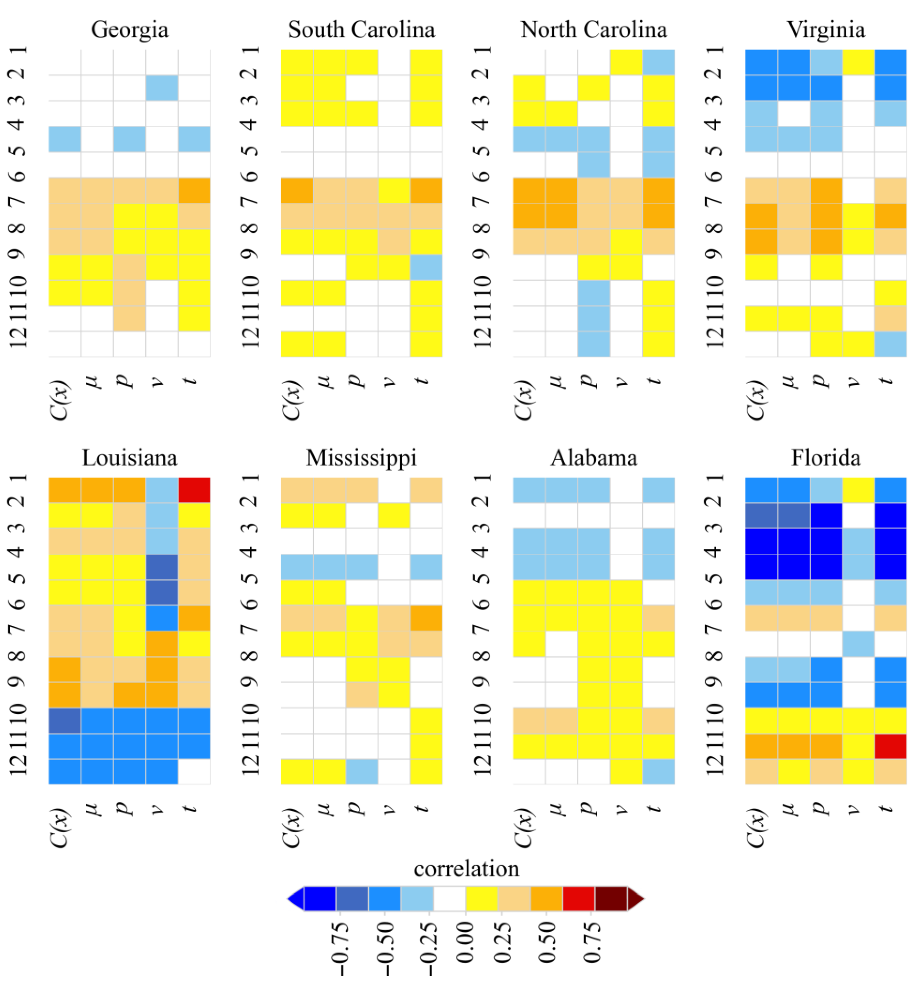
Figure 6.
Periodicity (C(x)) of streamflow droughts in consecutive months with isohyets of average monthly precipitation (mm).
Figure 6.
Periodicity (C(x)) of streamflow droughts in consecutive months with isohyets of average monthly precipitation (mm).

Figure 7.
First significant lag in monthly ACF distributions.

Figure 8.
First significant lag in monthly PACF distributions.
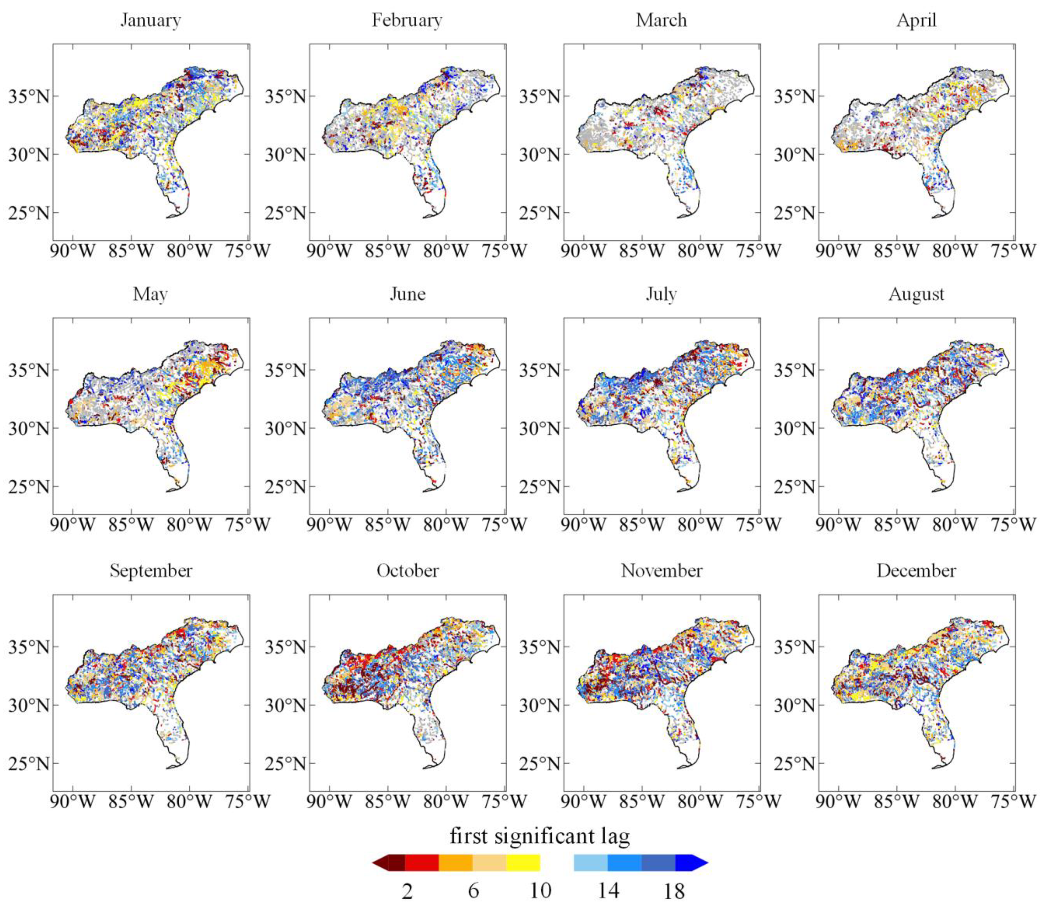
Figure 9.
Hurst exponent values for monthly series.


Table 1.
Percent of nodes with statistically significant lags of annual ACF and PACF.
| No Lag | 1st | 2nd | 3rd | 4th | 5th | 6th | 7th | 8th | 9th | 10th | 11th | 12th | 13th | 14th | 15th | 16th | 17th | 18th | 19th | 20th | |
|---|---|---|---|---|---|---|---|---|---|---|---|---|---|---|---|---|---|---|---|---|---|
| ACF | 83.82 | 7.92 | 0.86 | 0.96 | 0.72 | 2.02 | 0.17 | 0.80 | 0.09 | 0.28 | 0.32 | 0.22 | 1.56 | 0.15 | 0.01 | 0.04 | 0.01 | 0.02 | 0.01 | 0.00 | 0.02 |
| PACF | 26.77 | 8.86 | 3.96 | 1.17 | 3.95 | 4.66 | 1.92 | 2.35 | 3.54 | 2.64 | 3.63 | 2.11 | 2.56 | 3.05 | 2.23 | 3.35 | 3.12 | 4.50 | 5.80 | 3.26 | 6.59 |
Publisher’s Note: MDPI stays neutral with regard to jurisdictional claims in published maps and institutional affiliations. |
© 2022 by the authors. Licensee MDPI, Basel, Switzerland. This article is an open access article distributed under the terms and conditions of the Creative Commons Attribution (CC BY) license (https://creativecommons.org/licenses/by/4.0/).
Share and Cite
MDPI and ACS Style
Raczynski, K.; Dyer, J. Variability of Annual and Monthly Streamflow Droughts over the Southeastern United States. Water 2022, 14, 3848. https://doi.org/10.3390/w14233848
AMA Style
Raczynski K, Dyer J. Variability of Annual and Monthly Streamflow Droughts over the Southeastern United States. Water. 2022; 14(23):3848. https://doi.org/10.3390/w14233848
Chicago/Turabian StyleRaczynski, Krzysztof, and Jamie Dyer. 2022. "Variability of Annual and Monthly Streamflow Droughts over the Southeastern United States" Water 14, no. 23: 3848. https://doi.org/10.3390/w14233848
Note that from the first issue of 2016, this journal uses article numbers instead of page numbers. See further details here.