Evaluating Three Supervised Machine Learning Algorithms (LM, BR, and SCG) for Daily Pan Evaporation Estimation in a Semi-Arid Region

Abstract

Evaporation is one of the main components of the hydrological cycle, and its estimation is crucial and important for water resources management issues. Access to a reliable estimator tool for evaporation simulation is important in arid and semi-arid areas such as Iran, which lose more than 70% of their received precipitation by evaporation. Current research employs the Bayesian Regularization (BR) and Scaled Conjugate Gradient (SCG) algorithms for training the Multilayer Perceptron (MLP) model (as MLP-BR and MLP-SCG) and comparing their performance with the Levenberg–Marquardt (LM) algorithm (as MLP-LM). For this purpose, 16 meteorological variables were used on a daily scale; including temperature (5 variables), air pressure (4 variables), and relative humidity (6 variables) as input data sets, and pan evaporation as the target variable of the MLP model. The surveys were conducted during the period of 2006–2021 in Fars Province in Iran, which is a semi-arid region and has many natural lakes. Various combinations of input-target pairs were tested by several learning algorithms, resulting in seven input scenarios: (1) temperature-based (T), (2) pressure-based (F), (3) humidity-based (RH), (4) temperature–pressure-based (T-F), (5) temperature–humidity-based (T-RH), (6) pressure–humidity-based (F-RH) and (7) temperature–pressure–humidity-based (T-F-RH). The results indicated the relative superiority of the three-component scenario of T-F-RH, and a considerable weakness in the single-component scenario of RH compared with others. The best performance with a root mean square error (RMSE) equal to 1.629 and 1.742 mm per day and a Wilmott Index (WI) equal to 0.957 and 0.949 (respectively for validation and test periods) belonged to the MLP-BR model. Additionally, the amount of R² (greater than 84%), Nash-Sutcliff efficiency (greater than 0.8) and normalized RMSE (less than 0.1) all indicate the reliability of the estimates provided for the daily pan evaporation. In the comparison between the studied training algorithms, two algorithms, BR and SCG, in most cases, showed better performance than the powerful and common LM algorithm. The obtained results suggest that future researchers in this field consider BR and SCG training algorithms for the supervised training of MLP for the numerical estimation of pan evaporation by the MLP model.

1. Introduction

Evaporation is one of the most important components of the hydrological cycle, in which the liquid phase from the earth’s surface turns into atmospheric water vapor [1]. Determining the value of this variable in arid and semi-arid regions like Iran is very important because the average rainfall received in Iran is about one-third of the rainfall received in dry areas of the planet, and more than seventy percent of this amount is wasted by the process of evaporation. The evaporation rate is a non-linear hydrological process affected by several meteorological variables such as relative humidity, temperature, wind speed, and sunshine hours [2]. Evaporation is the main cause of water loss in reservoirs and soil moisture loss in agricultural fields. In Iran, the long-term average evaporation from the evaporation pan is 2250 mm per year, which means that a significant volume of the total freshwater stored in the dams, as well as soil water (soil moisture), can be lost due to evaporation [3]. As a result, in regions where water resources are limited, evaporation estimation is very important in irrigation planning and management practices using available meteorological parameters [1,4,5].

In general, direct and indirect methods are used to estimate evaporation. Direct methods include the use of class A pan, class U, and lysimeter [6]. In Iran, a class A evaporation pan uses in meteorological stations for direct measurement of evaporation. The evaporation rate measured from the pan indicates the evaporation potential, especially in dry and semi-arid areas. Researchers utilize evaporation pan coefficients to measure evaporation losses from dam reservoirs [7]. Direct methods of measuring evaporation are costly and have limitations in terms of space and time [5], hence conceptual models [8,9,10], experimental [11,12,13,14,15,16,17], and artificial intelligence methods [3,4,6,18] were developed for indirect estimation of evaporation. Among the conceptual models for simulating pan evaporation the PenPan model [10], the developed multilayer model [9], and PenPan-V2C and PenPan-V2S [8] have been employed by researchers. In the absence of required variables, these methods can add complexity to the simulation’s systematic and predictable errors. As a result, it is difficult to use many of these methods due to the lack of access to data and the lack of clear initial and boundary conditions [19].

In experimental models, pan evaporation is estimated by linear regression methods, while the evaporation process has a non-linear nature behavior in the nature [4]. Therefore, powerful and consistent estimation methods should be able to analyze nonlinear patterns of evaporation processes. Recently, many artificial intelligence models have been proposed to estimate evaporation, including the multilayer perceptron (MLP) model [3,6,18,20,21,22,23,24,25], support vector machine (SVM) model [26], M5tree model [27], adaptive neuro-fuzzy inference system (ANFIS) model [28], random forests (RF) model [6], relevance vector machine (RVM) model [29]. Additionally, various hybrid artificial intelligence-based models have been employed in evaporation simulation [30,31]. These cases are among artificial intelligence models that have a numerical nature and are not dependent on physical processes. As a result, they require less information (for example, initial or boundary conditions) and are also superior for decision-making in areas with sparse data compared with other types of parametric methods [30,32].

Table A1. Literature review on pan evaporation modeling cases using machine learning approaches.

Reference	Study Region	Models	Input Variables
Ashrafzadeh et al. [3]	Iran	MLP, SVM, SOMNN	Tmin, Tmax, T, RH, P, WS, S
Kişi [7]	USA	MLP, RBNN, MLR, SS	T, RS, WS, RH
Ali Ghorbani et al. [30]	Iran	MLP	Tmin, Tmax, WS, RH, S
Ghorbani et al. [36]	Iran	MLP, SVM	Tmin, Tmax, WS, RH, S
Kim et al. [33]	Iran	MLP, KSOFM, GEP, MLR	T, WS, RH, S, RS
Wang et al. [34]	China	MLP, GRNN, FG, LSSVM, MARS, ANFIS, MLR, SS	T, RS, S, RH, WS
Ashrafzadeh et al. [21]	Iran	MLP, SVM	Tmax, RHmax, RHmin, WS, S
Ehteram et al. [35]	Malaysia	MLP	T, WS, RH, RS
Al-Mukhtar [6]	Iraq	RF, QRF, SVM, MLR, ANN	Tmax, Tmin, RH, WS
Zounemat-Kermani et al. [28]	Turkey	NNARX, GEP, ANFIS	T, RS, RH, WS
Deo et al. [29]	Australia	RVM, ELM, MARS	Tmax, Tmin, RS, VP, P

in Appendix A presents some studies related to the application of artificial intelligence methods in pan evaporation estimation.

According to previous studies, the most effective meteorological variables for estimating evaporation include temperature, relative humidity, and air pressure. Additionally, the review of studies shows that a variety of artificial neural network models have been used to estimate evaporation from pans in different parts of the world. These methods have produced better results compared with experimental methods using available climate parameters [7,33,34]. Among the vast majority of studies conducted, MLP is one of the efficient artificial intelligence tools in pan evaporation simulation, and in recent years, the performance of this model in estimating evaporation has been improved by combining it with different algorithms [3,21,35,36]. In an MLP model, the design of the network architecture, including the number of neurons in each layer, the number of layers, driving functions, etc., is very important in the simulation process. This design can directly affect the ability of the neural network to solve the problem. One of the important steps in using MLP models is the training step, and during the neural network training process, the applied training function leads to solving a mathematical optimization problem. Additionally, the optimal weights of the network are calculated based on adjustable parameters [37].

Levenberg–Marquardt (LM) algorithm has been used in most evaporation estimation studies to train the MLP model [23,30,36,38]. It is claimed that this algorithm is stronger than many learning algorithms because of its ability to find the solution [39]. While there are two algorithms—Bayesian regularization (BR) and scaled conjugate gradient (SCG)—which have been very little discussed in evaporation estimation studies. In the current research, for the first time, the effectiveness of BR and SCG algorithms in MLP model training is investigated and their performance is compared with the ordinary LM algorithm. Additionally, in this research, a supervised training method is used for numerical modeling. In the current study, the evaporation modeling process was performed only based on temperature, air pressure, and relative humidity components, which have acceptable quality in their time series data. Another point is that previous studies [21,30,40] have performed pan evaporation modeling for the northern regions of Iran (the southern part of the Caspian Sea). The reason for this choice is the presence of significant surface water resources in that area, which makes the pan evaporation data closer to the actual evaporation rate. While in arid and semi-arid areas of Iran that have natural lakes and reservoir dams, the evaporation rate of the pan is very close to the actual evaporation rate from the surface of the lakes and reservoirs of the dams, but less has been conducted to model the evaporation in these areas of Iran. Therefore, the current research has investigated one of these areas in the south of Iran, which has very important natural lakes (from the hydrological, environmental, and ecological points of view).

2. Materials and Methods

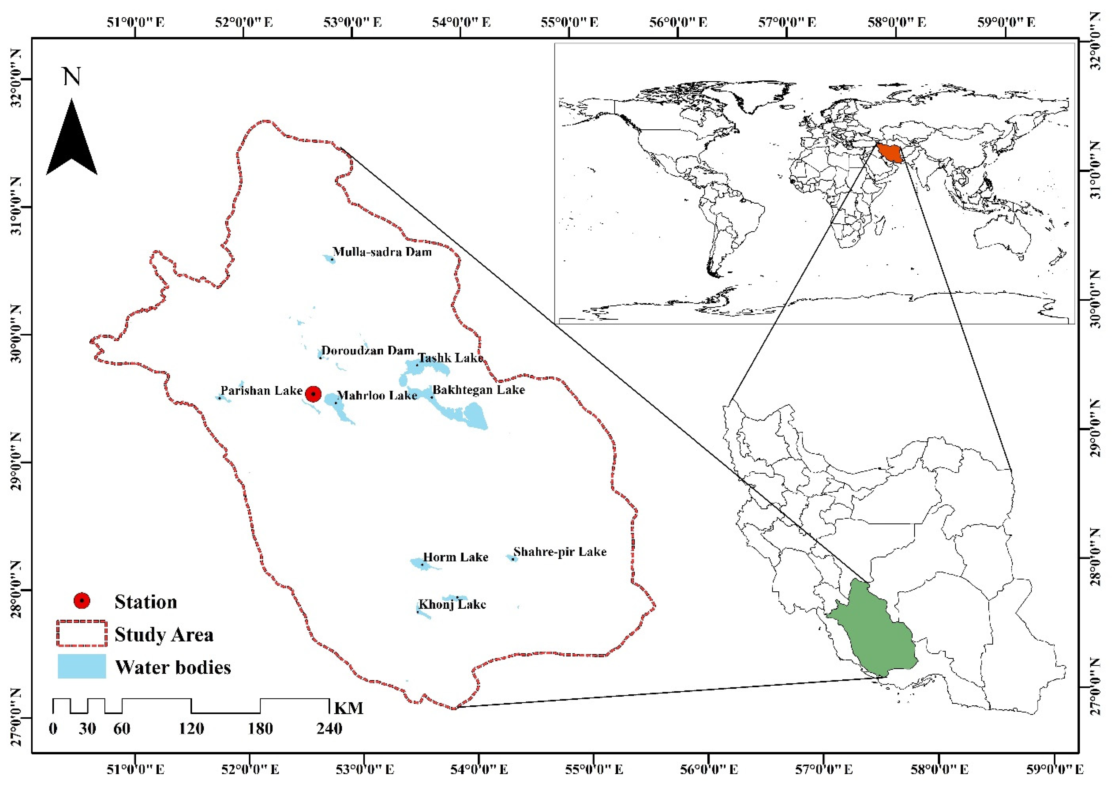
2.1. Study Region and the Data

Fars province was selected as the case study of the current study. This reign area is more than 122,608 square kilometers and is located in the south part of Iran. Fars Province is affected by mild winters and hot and dry summers. The studied region is located between latitudes of 27 degrees and 2 min and 31 degrees and 42 min north latitude and 50 degrees and 42 min and 55 degrees (Figure 1). The studied area has a wide variety of climatic zones, including cold and dry in the north, hot and dry in the south, temperate and humid areas in the central area, and hot and semi-humid in the west. Despite the diverse climatic regions of the province, its predominant climate is hyper-arid/temperate [41]. The plains of Fars Province are sedimentary basins located in the middle of the mountains, which are suitable for growing all kinds of agricultural products. On the other hand, the climate of this region (mild winters and hot and dry summers) has made it suitable for horticultural, agricultural, and livestock products. The important role of the studied area in the production of many agricultural products, including wheat, corn, cereals, oilseeds, dates, citrus fruits, figs, and sugar beet, has always brought unique capabilities that can bring many potential risks of water. Seasonal snow-covered heights in this region are the source of many rivers and springs that play a strengthening role in the irrigation of fields and water supply in urban areas. Moving from the south to the north of Fars Province, the plains decrease and the mountainous areas expand. In the southern and southwestern regions of the region, among the mountains, there are fertile plains of Shiraz, Kazeroon, Niriz, Marvdasht, etc., which are irrigated by rivers. These rivers eventually flow into Bakhtegan, Parishan, Maharlu, and Kaftar lakes. Due to the hot dry climate in Fars Province, evaporation from the free water surface is considered an important component in the water balance of these lakes, and its estimation can provide important information.

In this research, the Shiraz synoptic station is selected for evaporation modeling, which has a moderate semi-arid climate based on the Extended De-Martonne classification. The statistical characteristics of the data used are listed in

Table 1. Details of the daily datasets of the Shiraz site are obtained from the Iranian Meteorological Organization.

Variable	Training Period (2006–2017) *				Validation Period (2018–2019)				Validation Period (2020–2021)
	Min.	Max.	Average	STD.	Min.	Max.	Average	STD.	Min.	Max.	Average	STD.
Tmax (°C)	2.0	42.6	26.7	9.4	9.0	42.4	27.1	9.5	5.2	42.4	27.6	9.2
Tmin (°C)	−8.1	26.6	10.2	7.9	−6.0	27.8	10.5	7.9	−5.8	25.0	10.2	7.8
T (°C)	−1.1	34.7	19.0	9.0	0.9	35.5	19.3	9.2	1.5	34.0	19.4	9.0
Tdew (°C)	−16.7	16.7	0.8	4.9	−16.4	12.6	−0.1	5.0	−18.8	15.1	−1.1	5.4
Twet (°C)	−4.1	21.4	10.1	5.0	−1.5	18.4	10.0	4.7	−1.8	20.0	9.8	4.7
Fmax (mbar)	840.9	865.6	852.7	4.1	841.6	862.7	852.9	4.2	842.0	864.3	853.1	4.1
Fmin (mbar)	837.7	861.1	849.5	3.9	838.8	859.2	849.5	4.1	838.8	860.4	849.7	4.0
F (mbar)	839.9	862.8	851.0	3.9	840.5	860.6	851.2	4.1	840.7	861.7	851.3	3.9
VP (mbar)	5.7	56.9	26.2	13.5	7.8	58.9	26.7	14.4	7.0	55.5	26.8	13.9
RHmax (%)	14.0	100.0	60.1	20.6	11.0	100.0	59.1	24.2	14.0	100.0	56.5	24.8
RHmin (%)	2.0	93.0	19.4	14.6	2.0	97.0	18.5	16.3	1.0	98.0	16.1	14.9
RH (%)	7.3	98.3	36.8	18.2	6.6	98.9	36.4	20.6	7.3	99.3	33.8	20.0
RH03 (%)	12.0	100.0	58.0	19.9	11.0	100.0	56.3	23.5	13.0	100.0	53.8	23.7
RH09 (%)	2.0	100.0	23.9	17.4	2.0	100.0	23.3	19.0	2.0	100.0	20.5	18.3
RH15 (%)	2.0	100.0	28.9	19.7	2.0	100.0	28.3	21.6	1.0	100.0	26.1	21.2
Epan (mm)	0.0	18.8	7.0	3.9	0.1	17.8	6.7	4.2	0.1	18.2	6.8	4.2

Notes: * Min.: Minimum; Max.: Maximum; STD.: Standard deviation.

which covers daily data from 2006 to 2021. These data include 16 variables; maximum air temperature (Tmax), minimum air temperature (Tmin), mean air temperature (T), dew point temperature (Tdew), wet-bulb temperature (Twet), the maximum air pressure (Fmax), minimum air pressure (Fmin), mean air pressure (F), maximum relative humidity (RHmax), minimum relative humidity (RHmin), mean relative humidity (RH), relative humidity at 03:00 (RH03), relative humidity at 09:00 (RH09), relative humidity at 15:00:00 (RH15) and pan evaporation (Epan). Since the recorded data of solar radiation in most stations of Iran have low quality and a large number of outliers, the present research intends to present a model far from solar radiation.

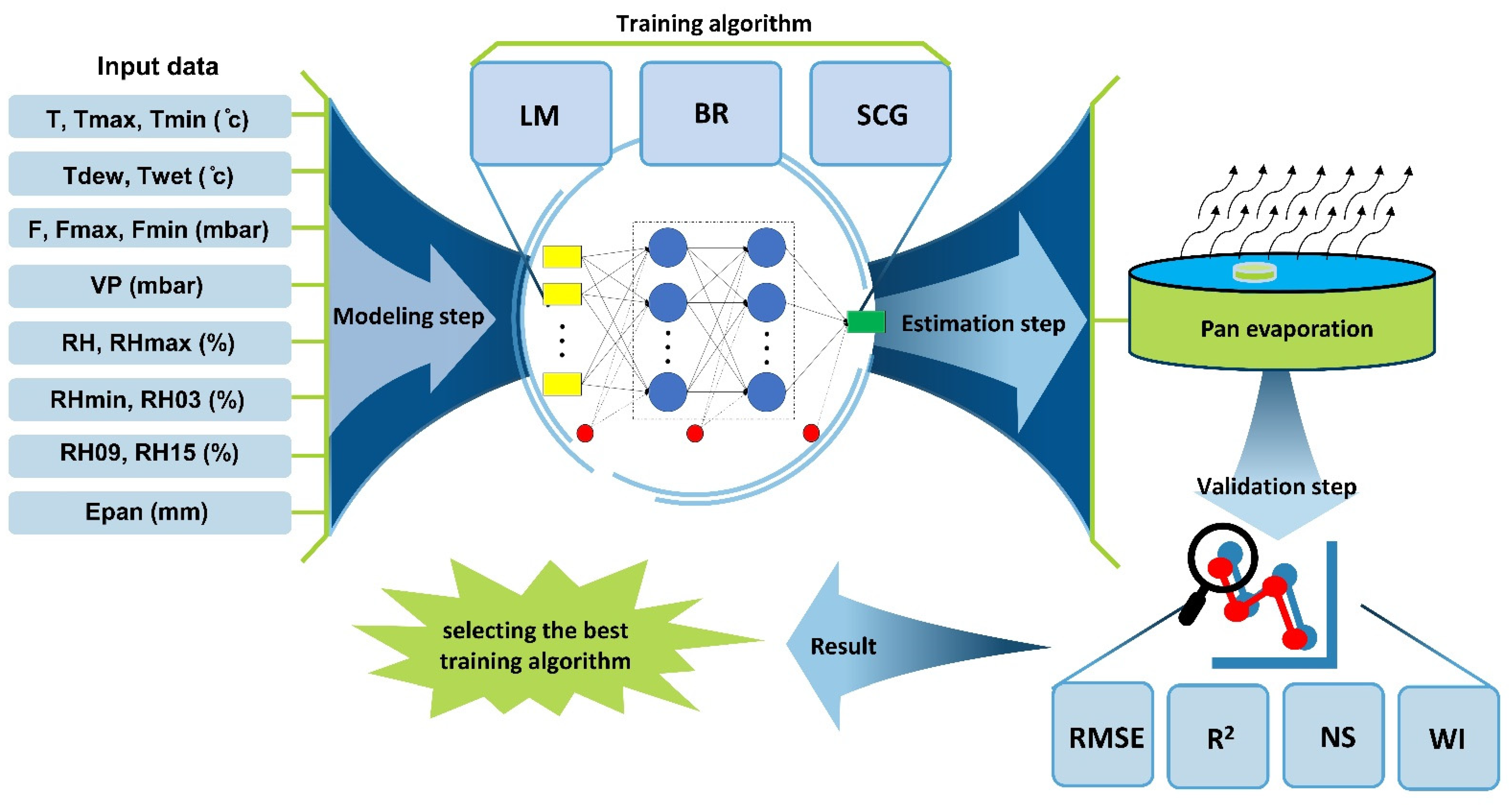
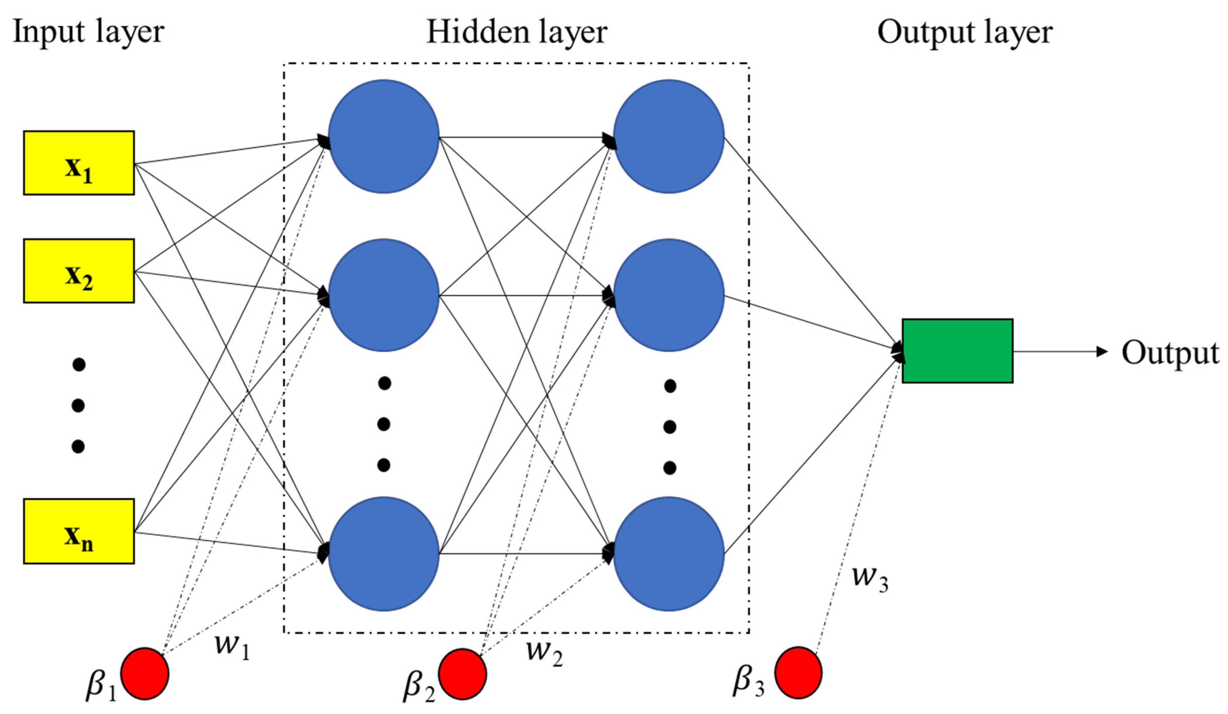
2.2. Multilayer Perceptron (MLP) Neural Network

The Multilayer Perceptron (MLP) model is one of the most common and practical models of connection between neurons in ANN [42]. This model consists of units, including an input layer, one or more hidden layers, an output layer, and a set of neurons or nodes for transferring information between layers. The number of neurons in the input and output layers is determined according to the number of input and output variables of the investigated system. Each neuron is connected to several nearby neurons with different weights that indicate the relative influence of the inputs. The weighted sum of inputs is transferred to hidden neurons using transfer functions. Additionally, the outputs of the hidden neurons also serve as inputs to the output neuron, where they undergo further transformation. The output of the MLP neural network can be expressed as Equation (1) [43].

$${\gamma }_{jk}=F_k\left({\displaystyle \sum }_{i=1}^{N_{k-1}}{w}_{ijk}{\gamma }_{i\left(k-1\right)}+{\beta }_{jk}\right)$$

(1)

where ${\gamma }_{jk}$ is the output of neuron j from layer k, ${\beta }_{jk}$ is the bias weight for neuron j in layer k, $w_{ijk}$ are model fitting parameters and $F_k$ are nonlinear activation transfer functions that may take different forms such as hyperbolic tangent sigmoid (tansig), Consider logarithmic sigmoid (logsig), saturated linear (satlin), and linear (purelin) [44]. Model fitting parameters ($w_{ijk}$) are link weights that were randomly selected at the beginning of the network training process. The MLP learning algorithm is in the form of backpropagation, and there are other types of backpropagation such as scaled conjugate gradient (SCG), Levenberg–Marquardt (LM), Bayesian regularization backpropagation (BR), gradient descent with variable learning rate backpropagation (GDX) and resilient backpropagation (RP) [45,46,47,48] which are usually used to find a set of optimal parameters for MLP models. Figure 2 shows the general structure of an MLP network with two hidden layers. In this study, in order to improve the estimation performance of MLP neural network for pan evaporation modeling by changing the number of hidden layers and the number of neurons in each hidden layer, different training algorithms such as LM, BR, and SCG were compared in evaporation estimation.

2.3. Learning Algorithms for MLP Neural Network

2.3.1. Levenberg–Marquardt (LM)

The Levenberg–Marquardt method was designed by Marquardt [49] and it can be used to increase the speed of second-order training without the need to calculate or approximate the Hessian matrix (such as Newton’s algorithm or Newton’s pseudo-algorithm). It was designed by Marquardt [49]. According to the Levenberg–Marquardt algorithm, the values of the weights are updated during an iterative process in the form of Equation (3). This algorithm is efficient for training smaller networks [50]. The LM learning algorithm has become increasingly popular because it can be easily implemented and changed to the GD or pseudo-Newton algorithm, and the learning can be adjusted automatically. The weight update equation in the LM algorithm is shown in Equation (2).

$${\theta }_{k+1}={\theta }_k-{\left[J_k^T{J}_k+\mu I\right]}^{-1}{J}_k{}^T{E}_k$$

(2)

where J represents the Jacobian matrix of the error vector E(θ) with a dimension, $J^{T }$ is the Tranhade matrix J, and I is the same matrix as the approximate Hessian matrix $J^{T }$. The gradient of the error function (namely E) increases or decreases according to the weight and bias parameters $\theta =\left\{{\beta }_j,w_{ij}\right\}$ and the adjustment parameter μ (damping coefficient) during each learning iteration to guide the optimization process (µ = 0.001 as the initial learning parameter). When the value of μ is very large, the Levenberg–Marquardt method approximates the gradient descent method. However, when μ is small, it is the same as the Gauss-Newton method. The advantage of this LM method is that it converges faster around the minimum and gives more accurate results.

2.3.2. Bayesian Regularization

The Bayesian regularization method is a combination of the Levenberg–Marquardt method along with multiple minimizations of weights to prevent the arbitrary increase in their values during iterations. In fact, in addition to error minimization, this algorithm also seeks to minimize the square of weights [45,51,52]. The algorithm uses BR and modifies all variables according to the LM function approximation method, as a result, the training objective function is defined as Equation (3) [43].

$$F=\alpha E_{\omega }+\beta E_D$$

(3)

where $E_{\omega }$ is the squared weights of the network, $E_D$ is the sum of the squared error of the network, and the values of α and β are the parameters of the objective function. Each of these parameters depends on the training of the network in reducing the remaining outputs or the volume of the network. The basic point of the adjustment method is how to select and optimize the parameters of the objective function through Bayesian statistical data. During the process of this algorithm, network weights are considered as random variables, then the prior distribution of network weights and training is considered as Gaussian distribution [45]. Equation (4) shows the Bayesian rule for optimizing the parameters of the objective function (α, and β) [53].

$$P\left(\alpha ,\beta |D,M\right)=\frac{P\left(D|\alpha ,\beta ,M\right)P\left(\alpha ,\beta |M\right)}{P\left(D|M\right)}$$

(4)

D represents the training data, M is the network model, and ω is the network weight.

2.3.3. Scaled Conjugate Gradient

In the SGC algorithm, unlike the basic backpropagation algorithm that changes the weights in the opposite direction of the gradient, the search is performed in conjugate directions, which has a faster convergence speed than the traditional backpropagation algorithm [54,55]. In the SCG algorithm, the closest next weight update vector $w_{t+1}$ to the current weight vector $w_t$ is expressed as Equation (5).

$$w_{t+1}=w_t-g_t{H}_t^{-1}$$

(5)

where $g_t=E\prime \left(w_t\right)$ is the gradient vector, $H_t=E″ \left(w_t\right)$ is the Hessian matrix E($w_t$), the product of $-g_t{H}_t^{-1}$ is known as Newton’s step, and its direction is denoted by the negative value, which is known as Newton’s direction [56]. If the Hessian matrix is positive definite and E($w_{t+1}$) is quadratic, Newton’s method directly reaches a local minimum in one step [56]. Otherwise, reaching the local minimum requires more iterations. To eliminate these drawbacks and speed up the learning rate, Møller [54] introduced time weight vector $w_{m,t}$ which is located between $w_{t+1}$ and $w_t$ and is expressed as relation 6.

$$w_{m,t}=w_t+{\gamma }_t{d}_t$$

(6)

where $d_t=-g_t$ is the conjugate direction vector of the time weight vector in the t iteration and ${\gamma }_t$ is the size of the time weight update step, which is called the short step size, so that $0<{\gamma }_t\ll 1$. The actual weight update is calculated as Equation (7).

$$w_{t+1}=w_t+{\alpha }_t{d}_t$$

(7)

where $w_{t+1}$ is the next weight update vector; $w_t$ Current weight vector and ${\alpha }_t$ is the actual weight update step size, which is called long step size and is determined as Equation (8).

$${\alpha }_t=\frac{-d_t^T{E}^t\left(w_t\right)}{d_t^T{s}_t}$$

(8)

$$s_t=E″\left(w_t\right)d_t\approx \frac{E\prime \left(w_{m,t}\right)-E\prime \left(w_t\right)}{{\gamma }_t}$$

(9)

where $s_t$ is second-order information; and ${\alpha }_t$ is the initial step size. To determine ${\alpha }_t$, $s_t$, the second-order information must be obtained from the first-order gradients [54]. Therefore, in an SCG algorithm, in each iteration, the time weights $w_{m,t}$ are first calculated using the short step size ${\gamma }_t$ (Equation (6)), and then the time weights are used to find the long step size ${\alpha }_t$ (Equations (8) and (9)). The final weight update is calculated using Equation (7).

2.4. Evaluating the Estimations

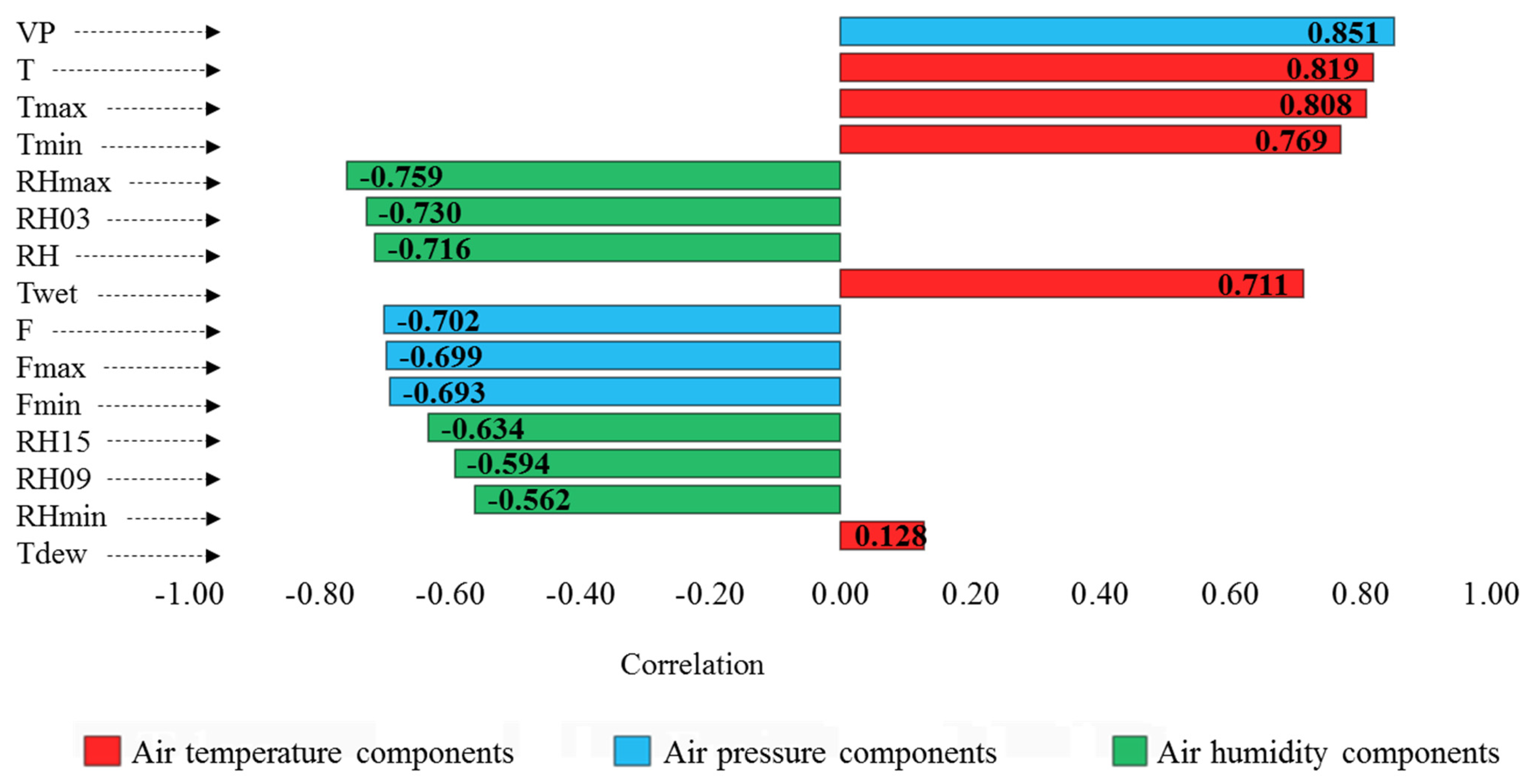
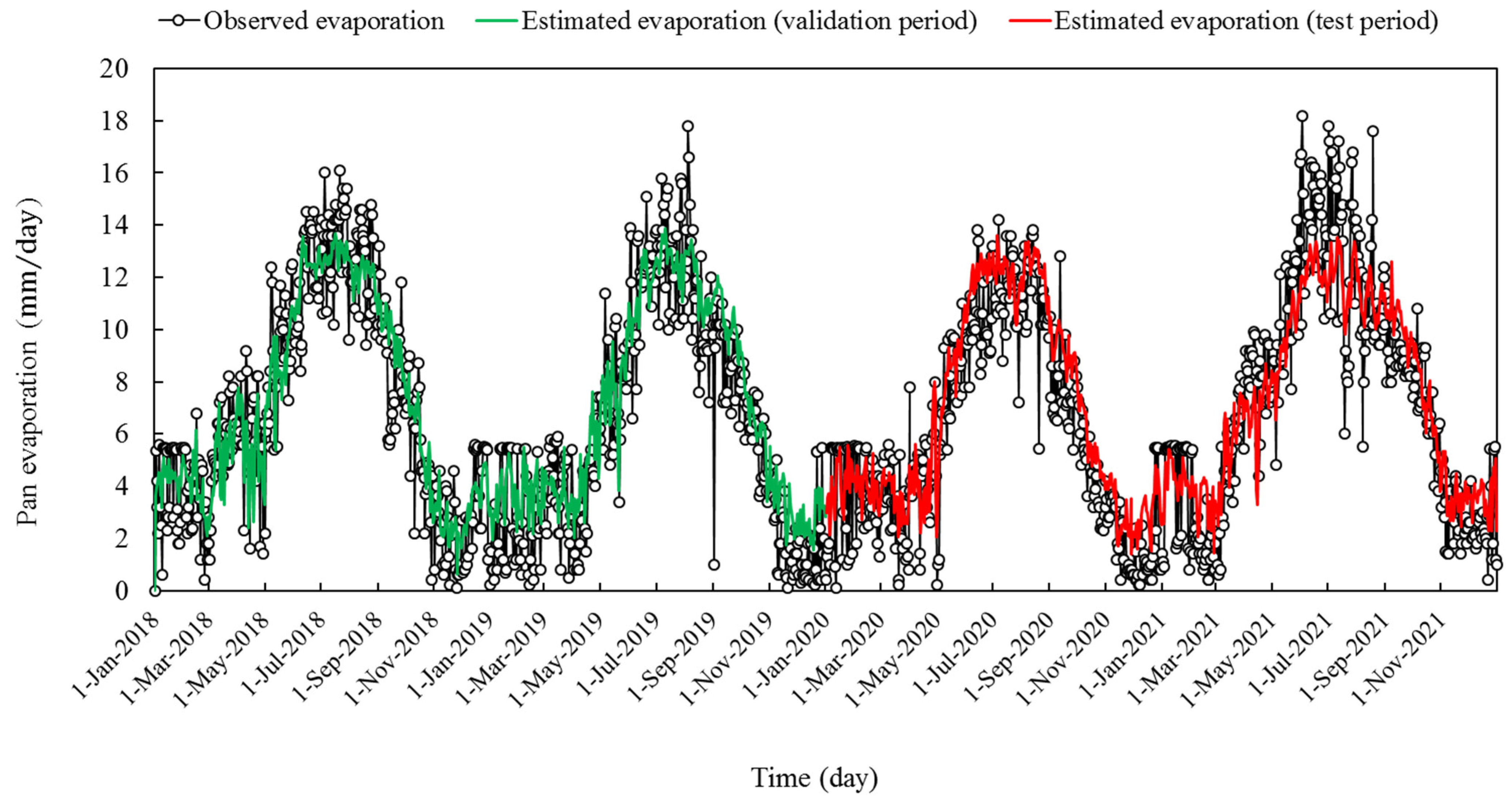
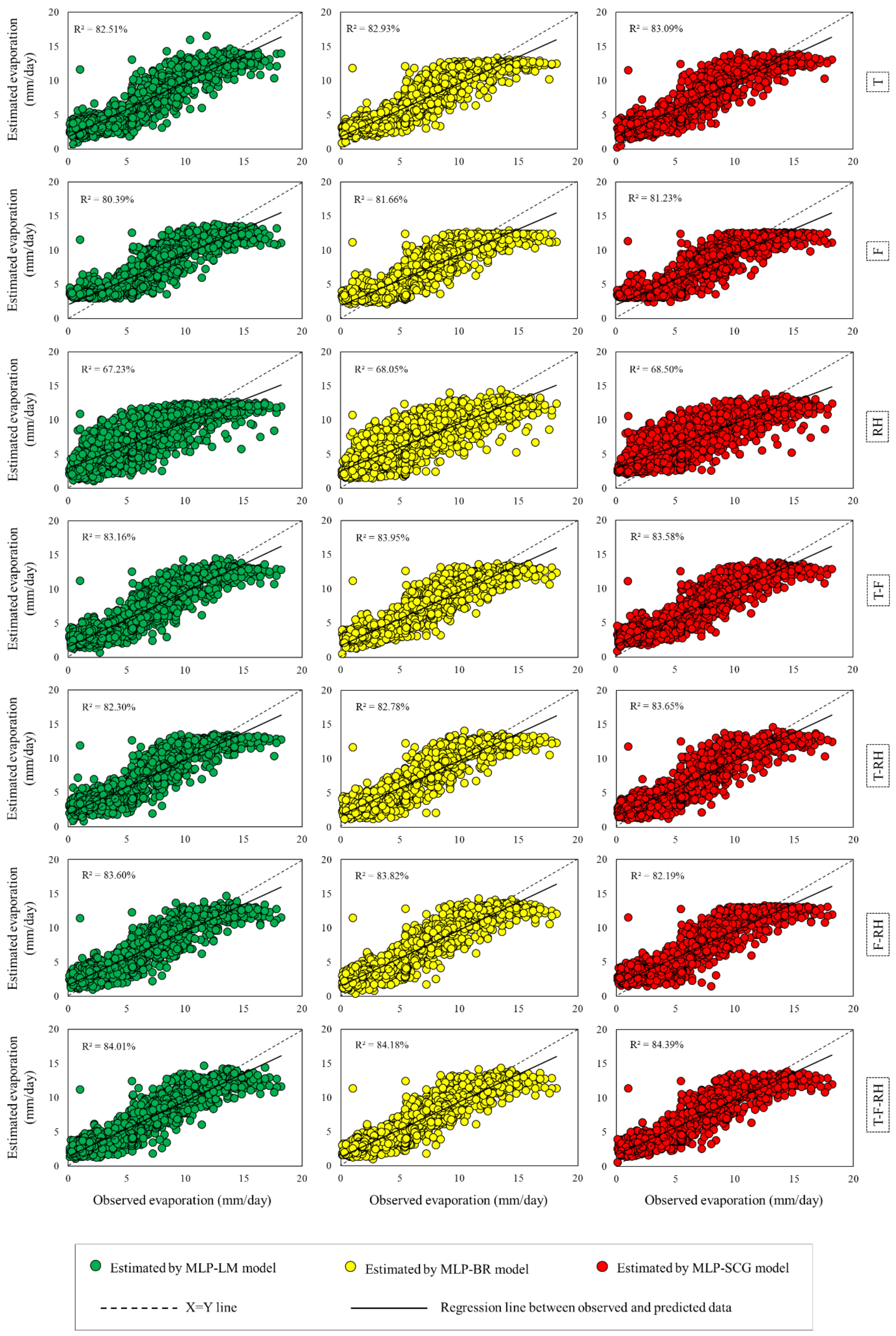
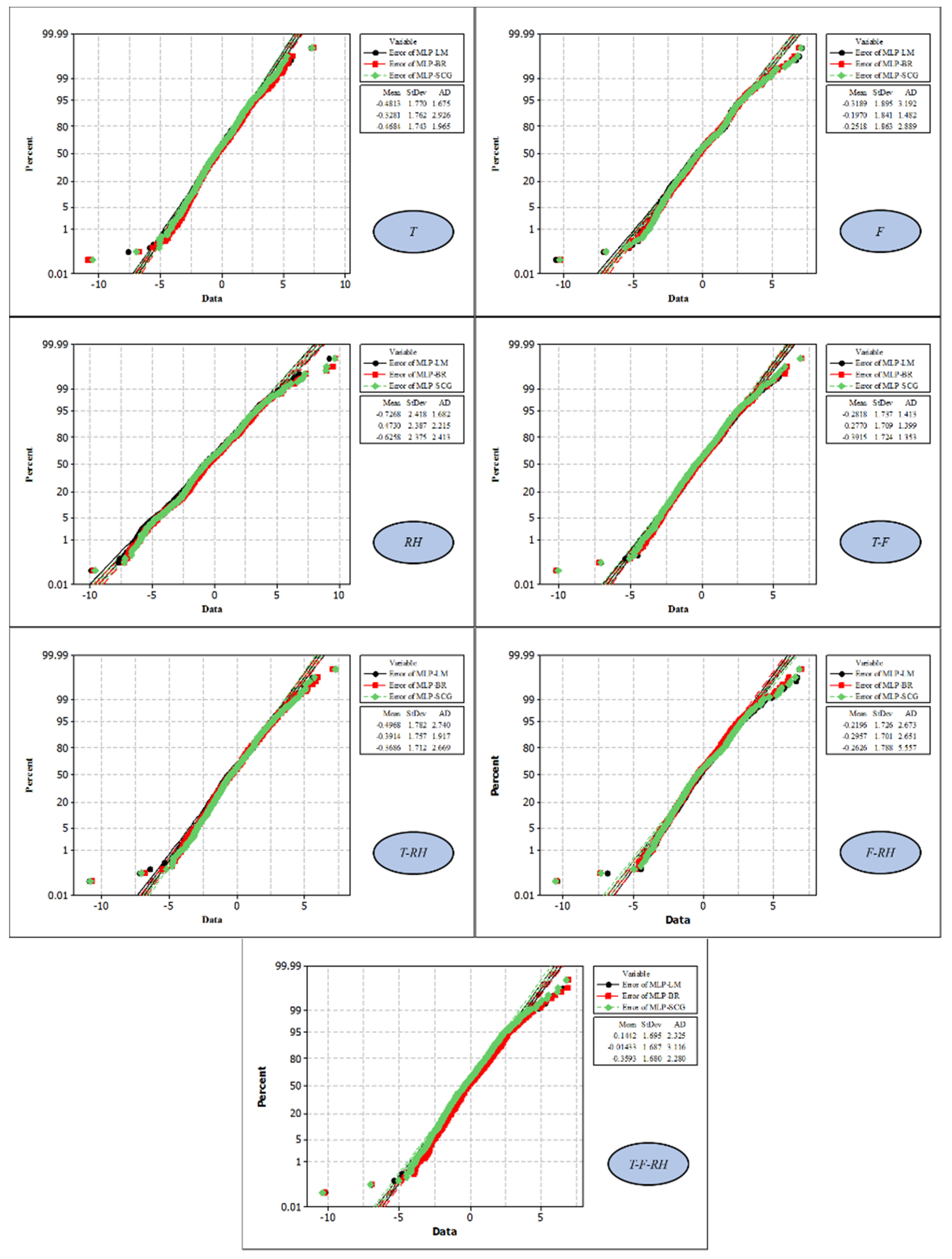
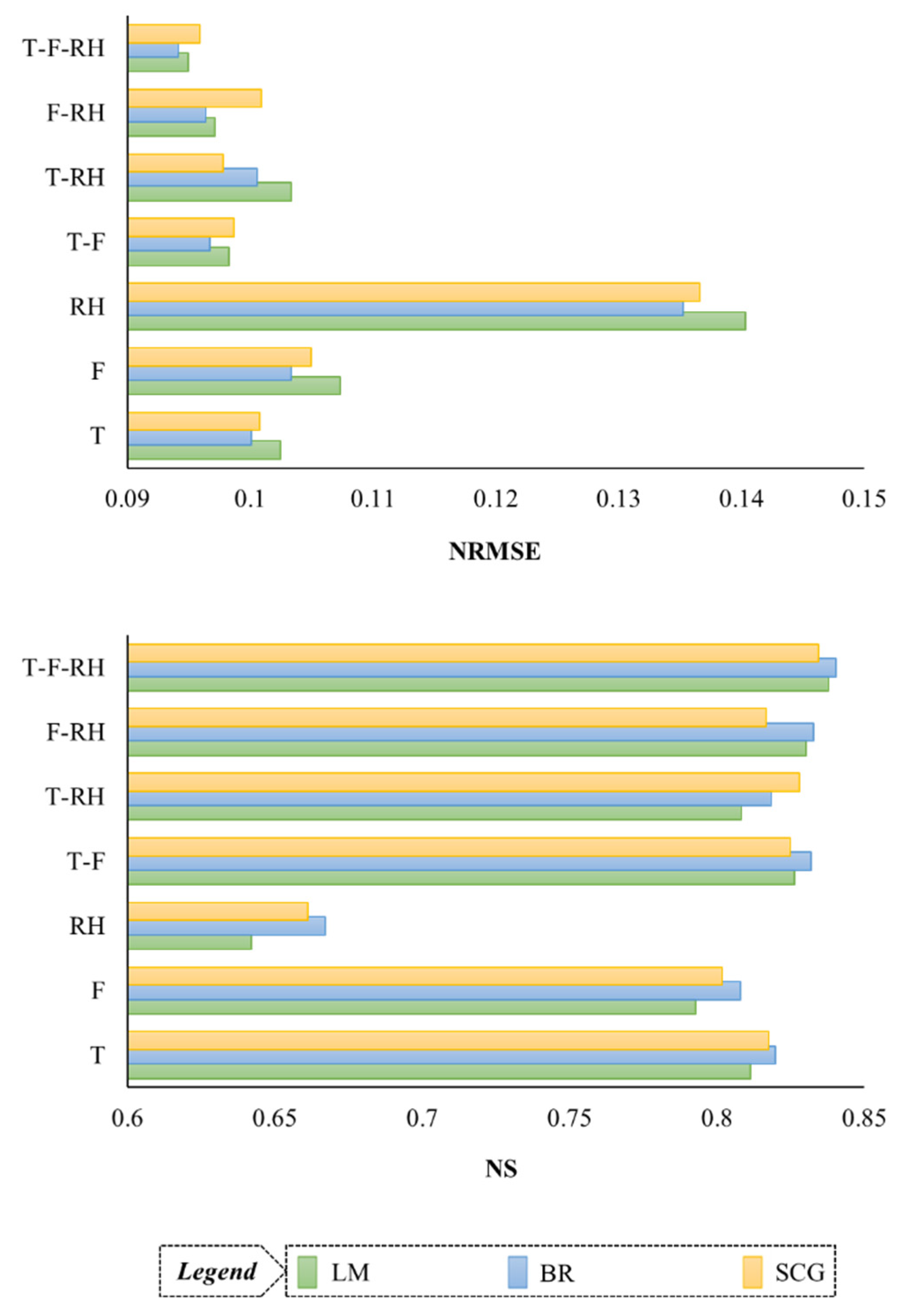
In this research, in order to evaluate the accuracy of evaporation simulation, the error criteria including Root Mean Square Error ($RMSE$), coefficient of determination ($R^2$), Nash Sutcliff ($NS$), and Willmott’s index of agreement (WI) were used, which are defined as follows.

$$RMSE=\sqrt{\frac{1}{n}{\displaystyle \sum }_{i=1}^n{\left(O_i-E_i\right)}^2}, 0<RMSE<+\infty$$

(10)

$$R^2={\left[\frac{{{\displaystyle \sum }}_{i=1}^n\left(O_i-\overline{O}\right)\left(E_i-\overline{E}\right)}{\sqrt{{{\displaystyle \sum }}_{i=1}^n{\left(O_i-\overline{O}\right)}^2}\ast \sqrt{{{\displaystyle \sum }}_{i=1}^n{\left(E_i-\overline{E}\right)}^2}}\right]}^2, 0<R^2<+1$$

(11)

$$NS=1-\frac{{{\displaystyle \sum }}_{i=1}^n{\left(O_i-E_i\right)}^2}{{{\displaystyle \sum }}_{i=1}^n{\left(O_i-\overline{O}\right)}^2}, -\infty <NS<+1$$

(12)

$$WI=1-\frac{{{\displaystyle \sum }}_{i=1}^n{\left(O_i-E_i\right)}^2}{{{\displaystyle \sum }}_{i=1}^n{\left(\left|O_i-\overline{O}\right|+\left|E_i-\overline{O}\right|\right)}^2}, -\infty <NS<+1$$

(13)

In these equations, $O_i$ is the observed data value on day i, $E_i$ is the estimated data value on the day i, $\overline{O}$ is the average of the observed values, $\overline{E}$ is the average of the estimated values, and n is the number of days under study. The closer the $RMSE$ values are to zero and $NS$, $R^2$, and $WI$ values are to one, the more accurate the estimation of the model is. The general stages of modeling in the present research can be seen in the form of a flowchart in Figure 3.

3. Results

For any time series simulation, it is necessary to choose the input combinations for the modeling process. In this research, air temperature (5 variables), air pressure (4 variables), and air humidity (6 variables) were used as inputs of machine learning estimator tools for estimating pan evaporation. The dependence of these variables on pan evaporation was evaluated separately by Pearson’s correlation test. The results are displayed in Figure 4.

In this diagram (Figure 4), the correlation coefficients are arranged according to intensity. Among these, the highest correlation coefficient belongs to the VP variable and the lowest one belongs to the Tdew variable. All variables have a significant correlation with pan evaporation at the confidence level of 0.01. The temperature components have a direct correlation, and the humidity components have an inverse correlation with pan evaporation. In the components related to air pressure, the VP variable in the direct direction, and the F, Fmax, and Fmin variables in the reverse direction are related to pan evaporation. The input scenarios were arranged based on seven combinations of the aforementioned variables. Therefore, the scenarios are temperature-based (only temperature variables), pressure-based (only pressure variables), humidity-based (only relative humidity variables), temperature–pressure-based (temperature and pressure variables), temperature–humidity-based (temperature and humidity variables), pressure–humidity-based (variables of pressure and humidity) and temperature–pressure–humidity-based (variables of temperature, pressure, and humidity) are considered (according to

Table 2. Analyzing the input scenarios by multiple linear regression.

Components	Scenario	Inputs	R2
Temperature (T)	S1	T	67.1%
	S2	T, Tmax	67.1%
	S3	T, Tmax, Tmin	67.4%
	S4	T, Tmax, Tmin, Twet	72.4%
	S5 *	T, Tmax, Tmin, Twet, Tdew	74.4%
Pressure (F)	S6	VP	72.4%
	S7	VP, F	73.4%
	S8	VP, F, Fmax	73.5%
	S9	VP, F, Fmax, Fmin	73.5%
Relative humidity (RH)	S10	RHmax	57.7%
	S11	RHmax, RH03	57.7%
	S12	RHmax, RH03, RH	57.8%
	S13	RHmax, RH03, RH, RH15	57.8%
	S14	RHmax, RH03, RH, RH15, RH09	58.9%
	S15	RHmax, RH03, RH, RH15, RH09, RHmin	59.1%
Temperature and pressure (T–F)	S16	VP, T	73.2%
	S17	VP, T, Tmax	73.2%
	S18	VP, T, Tmax, Tmin	73.4%
	S19	VP, T, Tmax, Tmin, Twet	75.4%
	S20	VP, T, Tmax, Tmin, Twet, F	76.1%
	S21	VP, T, Tmax, Tmin, Twet, F, Fmax	76.3%
	S22	VP, T, Tmax, Tmin, Twet, F, Fmax, Fmin	76.3%
	S23	VP, T, Tmax, Tmin, Twet, F, Fmax, Fmin, Tdew	76.5%
Temperature and relative humidity (T–RH)	S24	T, Tmax, Tmin, RHmax	70.4%
	S25	T, Tmax, Tmin, RHmax, RH03	70.4%
	S26	T, Tmax, Tmin, RHmax, RH03, RH	70.5%
	S27	T, Tmax, Tmin, RHmax, RH03, RH, Twet	73.6%
	S28	T, Tmax, Tmin, RHmax, RH03, RH, Twet, RH15	73.6%
	S29	T, Tmax, Tmin, RHmax, RH03, RH, Twet, RH15, RH09	73.6%
	S30	T, Tmax, Tmin, RHmax, RH03, RH, Twet, RH15, RH09, RHmin	73.7%
	S31	T, Tmax, Tmin, RHmax, RH03, RH, Twet, RH15, RH09, RHmin, Tdew	75.1%
Pressure and relative humidity (F–RH)	S32	VP, RHmax	74.3%
	S33	VP, RHmax, RH03	74.4%
	S34	VP, RHmax, RH03, RH	74.4%
	S35	VP, RHmax, RH03, RH, F	75.6%
	S36	VP, RHmax, RH03, RH, F, Fmax	75.7%
	S37	VP, RHmax, RH03, RH, F, Fmax, Fmin	75.7%
	S38	VP, RHmax, RH03, RH, F, Fmax, Fmin, RH15	75.8%
	S39	VP, RHmax, RH03, RH, F, Fmax, Fmin, RH15, RH09	75.8%
	S40	VP, RHmax, RH03, RH, F, Fmax, Fmin, RH15, RH09, RHmin	75.8%
Temperature, pressure and relative humidity (T–F–RH)	S41	VP, T, Tmax, Tmin, RHmax	75.6%
	S42	VP, T, Tmax, Tmin, RHmax, RH03	75.7%
	S43	VP, T, Tmax, Tmin, RHmax, RH03, RH	75.8%
	S44	VP, T, Tmax, Tmin, RHmax, RH03, RH, Twet	75.9%
	S45	VP, T, Tmax, Tmin, RHmax, RH03, RH, Twet, F	76.7%
	S46	VP, T, Tmax, Tmin, RHmax, RH03, RH, Twet, F, Fmax	76.7%
	S47	VP, T, Tmax, Tmin, RHmax, RH03, RH, Twet, F, Fmax, Fmin	76.7%
	S48	VP, T, Tmax, Tmin, RHmax, RH03, RH, Twet, F, Fmax, Fmin, RH15	76.8%
	S49	VP, T, Tmax, Tmin, RHmax, RH03, RH, Twet, F, Fmax, Fmin, RH15, RH09	76.8%
	S50	VP, T, Tmax, Tmin, RHmax, RH03, RH, Twet, F, Fmax, Fmin, RH15, RH09, RHmin	76.8%
	S51	VP, T, Tmax, Tmin, RHmax, RH03, RH, Twet, F, Fmax, Fmin, RH15, RH09, RHmin, Tdew	76.8%

Notes: * The bold rows refer to the best input scenarios in each component.

). In each scenario, the compounds were sorted based on the intensity correlation, which finally included 51 scenarios (S1–S51). Meanwhile, to reduce the workload, the multiple linear regression method was used to select the best input combination of the MLP model in each component arrangement. The results of this evaluation are shown in Table 2.

In Table 2, the best input combination of each component arrangement was selected based on the R² value, which can be seen in bold in the table. Therefore, on this basis, from now on, in the entire article, the scenarios related to each arrangement of components with the symbols T (temperature-based), F (pressure-based), RH (humidity-based), T-F (temperature–pressure-based), T-RH (temperature–humidity-based), F-RH (pressure–humidity-based) and T-F-RH (temperature–pressure–humidity-based) are shown (according to the components column in Table 2). It should be noted that according to the principle of parsimony, in cases where the R² value obtained by the multiple linear regression method did not change significantly, the scenario with the least number of input variables was considered the selected scenario. For example, in base pressure scenarios (F), scenarios S7 and S9 have R² equal to 73.4% and 73.5%, respectively. In this case, the difference in R² is very small and can be ignored, therefore, considering that S7 with 2 variables and S9 with 4 variables achieved this amount of R², the scenario with the least number of input variables (i.e., S7) was chosen as the best F scenario. Or in the T-F-RH scenarios, the S45 scenario with 9 variables achieved R² equal to 76.7%. Meanwhile, the S51 scenario with 15 variables could only improve the performance by 0.1% (R² = 76.8%); Therefore, it is obvious that based on parsimony, the S45 scenario is introduced as the best scenario of T-F-RH.

After selecting the input scenarios from each component (the bold rows of Table 2), the input combinations are applied to the MLP neural network. In this part, LM, BR, and SCG algorithms are considered for MLP model training, respectively. The arrangement of the MLP model, including the number of hidden layers, the number of neurons in each layer, and the type of transfer function inside the neurons were selected by trial and error. The results showed that the investigated data are most compatible with the arrangement of two hidden layers and the satlin (saturate linear transfer function) and tansig (tangent hyperbolic sigmoid transfer function) transfer functions. The modeling results of the mentioned three training algorithms are evaluated separately by RMSE and WI criteria (

Table 3. Evaluation metrics for the pan evaporation modeling of MLP, learned by Levenberg–Marquardt algorithm (MLP-LM).

Input Scenario	Transfer Function	Network Makeup *	Train		Validation		Test
			RMSE	WI	RMSE	WI	RMSE	WI
T	satlin	12-10-1	1.853	0.932	1.836	0.945	1.832	0.944
F	satlin	15-10-1	1.939	0.924	1.879	0.939	1.962	0.931
RH	satlin	12-12-1	2.395	0.871	2.295	0.907	2.733	0.866
T-F	satlin	15-10-1	1.773	0.939	1.739	0.951	1.779	0.947
T-RH	satlin	18-12-1	1.844	0.934	1.838	0.945	1.861	0.942
F-RH	tansig	18-18-1	1.799	0.935	1.686	0.953	1.791	0.945
T-F-RH **	tansig	12-12-1	1.797	0.936	1.652	0.956	1.747	0.949

Notes: * This column shows the number of hidden layers and the neurons. For example, 12-1 says that the network makeup includes a single hidden layer with neurons in it and an output layer with 1 neuron. ** The bold row indicates the best estimation performance.

,

Table 4. Evaluation metrics for the pan evaporation modeling of MLP, learned by Bayesian regularization algorithm (MLP-BR).

Input Scenario	Transfer Function	Network Makeup *	Train		Validation		Test
			RMSE	WI	RMSE	WI	RMSE	WI
T	tansig	12-10-1	1.887	0.928	1.777	0.948	1.807	0.943
F	satlin	12-12-1	1.892	0.928	1.821	0.943	1.880	0.937
RH	satlin	10-10-1	2.410	0.872	2.199	0.916	2.646	0.874
T-F	satlin	15-10-1	1.815	0.934	1.697	0.953	1.765	0.946
T-RH	tansig	12-10-1	1.810	0.935	1.778	0.949	1.821	0.945
F-RH	tansig	18-15-1	1.832	0.934	1.660	0.956	1.790	0.947
T-F-RH **	tansig	12-12-1	1.836	0.934	1.629	0.957	1.742	0.949

Notes: * This column shows the number of hidden layers and the neurons. For example, 12-1 says that the network makeup includes a single hidden layer with neurons in it and an output layer with 1 neuron. ** The bold row indicates the best estimation performance.

and

Table 5. Evaluation metrics for the pan evaporation modeling of MLP, learned by scaled conjugate gradient algorithm (MLP-SCG).

Input Scenario	Transfer Function	Network Makeup *	Train		Validation		Test
			RMSE	WI	RMSE	WI	RMSE	WI
T	tansig	12-10-1	1.879	0.929	1.792	0.948	1.816	0.944
F	tansig	12-12-1	1.915	0.926	1.832	0.941	1.927	0.933
RH	tansig	10-10-1	2.394	0.867	2.245	0.909	2.648	0.869
T-F	satlin	12-10-1	1.823	0.934	1.738	0.951	1.796	0.945
T-RH	satlin	18-15-1	1.853	0.932	1.722	0.953	1.778	0.947
F-RH	satlin	10-10-1	1.874	0.930	1.747	0.950	1.865	0.941
T-F-RH **	satlin	12-12-1	1.814	0.935	1.668	0.955	1.766	0.947

Notes: * This column shows the number of hidden layers and the neurons. For example, 12-1 says that the network makeup includes a single hidden layer with neurons in it and an output layer with 1 neuron. ** The bold row indicates the best estimation performance.

).

Examining the evaluation table of the MLP model trained with the LM algorithm (Table 5), shows that according to the WI criterion, the estimates of this model have been acceptable in most cases (0.9 < WI < 1). The humidity-based single-component scenario provided the weakest estimation of pan evaporation among the input scenarios with RMSE equal to 2.295 and 2.733 mm per day, and WI equal to 0.907 and 0.866 for the validation and test phases, respectively. Among the two-component scenarios, the best performance belonged to the pressure–humidity-based scenario; with RMSE equal to 1.686 and 1.791 mm per day, and WI equal to 0.953 and 0.945 for the validation and test phases, respectively. Among all seven examined scenarios, the temperature–pressure–humidity-based three-component scenario presented the best performance, in which RMSE equals 1.652 and 1.747 mm per day, and WI equals 0.956 and 0.949, respectively for validation and test periods are reported. The overlapping of the outputs of this scenario with the observed values of pan evaporation can be seen in the time series plot (Figure 5).

Examining the evaluation table of the MLP model trained with the BR algorithm (Table 4), shows that according to the WI criteria, the estimates of this model have been acceptable in most cases (0.9 < WI < 1). Among the input scenarios, the humidity-based single-component scenario with RMSE equal to 2.199 and 2.646 mm per day, and WI equal to 0.916 and 0.874 for the validation and test phases, respectively, provided the weakest estimation of pan evaporation. Among the two-component scenarios, the best performance belonged to the pressure–humidity-based scenario (with a slight advantage over the temperature–pressure-based scenario); with RMSE equal to 1.660 and 1.790 mm per day, and WI equal to 0.956 and 0.947 for the validation and test phases, respectively. Among all the input scenarios, the three-component temperature–pressure–humidity-based scenario provided the best estimation of pan evaporation, with RMSE equal to 1.629 and 1.742 mm/day, and WI equal to 0.957 and 0.949, respectively for Validation and test courses. The overlapping of the outputs of this scenario with the observed values of pan evaporation can be seen in the time series plot (Figure 6).

The evaluation table of the MLP model trained with an SCG algorithm (Table 5) shows that according to WI, the evaporation estimated by this model is acceptable in most cases (0.9 < WI < 1). Among the analyzed input scenarios, the weakest performance belonged to the humidity-based scenario, where RMSE is equal to 2.245 and 2.648 mm per day, and WI is equal to 0.909 and 0.869 for the validation and test phases, respectively. The temperature–humidity-based scenario provided the best estimation by RMSE equal to 1.722 and 1.778 mm per day, and WI was equal to 0.953 and 0.947 for the validation and test phases, respectively. Among all seven examined scenarios, the temperature–pressure-humidity-based three-component scenario had the lowest error in pan evaporation estimation, so that RMSE was equal to 1.668 and 1.766 mm per day, and WI was equal to 0.955 and 0.947. The order for the validation and test courses was achieved. The overlapping of the outputs of this scenario with the observed values of pan evaporation can be seen in the time series plot (Figure 7).

Scatter plots (Figure 8) have been used to check the correlation between the evaporation estimates and the actual data measured from the evaporation pan, which will be discussed below. This diagram is drawn simultaneously for the two phases of validation and test (1 January 2018–31 December 2021).

By observing the scatter plots in Figure 8, it can be seen that the estimations and observations of evaporation have a direct correlation with each other. The distribution of the points is also such that they have a relatively high concentration around the regression lines and indicate a favorable correlation between the estimated-observed samples. Additionally, the slope difference between the regression lines and the 1:1 line is very small and acceptable. The comparison of R² among the three models MLP-LM, MLP-BR, and MLP-SCG shows that the models have minor performance differences. However, in almost all 7 scenarios examined, this minor difference indicates the superiority of BR and SCG algorithms in MLP model training, compared with the common LM training algorithm. According to these graphs, the weakest performance is observed in the humidity-based single-component scenario (RH) where R² is equal to 67.23%, and it is the result of MLP model training by the LM algorithm. The best estimates presented always belong to the temperature–pressure–humidity-based three-component scenario (T-F-RH), which has the highest R² among all scenarios. In this scenario, the best training of the MLP model was provided by the SCG-supervised algorithm and the weakest was provided by the LM (R² equal to 84.39% and 84.01%, respectively). Of course, in the meantime, the two-component scenarios such as T-F and F-RH also had relatively good performances, in which the amount of R² was very close to the three-component scenario of T-F-RH (T-F: 83.16% < R² < 83.95%; F-RH: 82.19% < R² < 83.82%). To check the performance among the scenarios, probability plots were drawn for the error of the models (Figure 9). This diagram is drawn simultaneously for the training and testing phases.

In these graphs (Figure 9), the error rate of the model is displayed on the x-axis, and the percentage of frequency in that error rate is displayed on the y-axis. This operation was carried out for the outputs of all three educational algorithms under review, and their mean and standard deviation were also calculated. Additionally, Anderson Darling (AD) test was used to check the closeness of error probability distribution to normal distribution. The statistics of this test are shown with AD in the graphs (the smaller the AD is, the closer the error distribution is to the normal distribution). The AD statistic shows that the errors resulting from the LM training algorithm are better than the BR and SCG algorithms in two scenarios (T and RH) and are weaker than them in three scenarios (F, T-F, and T-RH). Based on this, the BR training algorithm performed best in three scenarios (F, T-RH, and F-RH), and performed the weakest in two scenarios (T and T-F-RH). The SCG algorithm is also evaluated better than the other two algorithms in the T-F and T-F-RH scenarios, and weaker than them in the RH and F-RH scenarios. The closest distribution of pan evaporation estimation errors to the normal distribution is related to the MLP-SCG model under the T-F scenario, where AD is equal to 1.353. In the comparison of mean and standard deviation between the errors of the estimates provided for pan evaporation, the T-F-RH scenario shows the best situation (the closer these values are to zero, the better the performance of the model is evaluated). Among these, the best evaporation belongs to the MLP-BR model, in which the average error of evaporation estimation is very close to zero (−0.014 mm per day) and its standard deviation is reported as 1.687 mm per day. To compare the performance of the input scenarios, the evaluation criteria of NRMSE and NS have been used, which will be analyzed in the form of bar charts (Figure 10).

In Figure 10, two measures NRMSE and NS were considered for the performance of all three training algorithms. At first glance, it is clear that the humidity-based (RH) scenario has achieved the weakest estimate of evaporation; According to NRMSE classes (0.1 < NRMSE < 0.2), its performance is evaluated as relatively well. Additionally, the amount of NS in this scenario is less than 0.75, while in the other 6 scenarios, it is in the range of 0.8 and above. In other scenarios, the amount of NRMSE also approaches 0.1 (F, T, and T-RH) and less (T-F, F-RH, and T-F-RH). It can be seen that the best performance belongs to the three-component scenario of T-F-RH, which in terms of NRMSE classes (NRMSE < 0.1), the related performances are evaluated as excellent. The amount of NS also reaches its maximum in this scenario (0.840–0.834). In the comparison between the studied training algorithms, it can be clearly seen by referring to both NS and NRMSE criteria that in 6 scenarios (T, F, RH, T-F, F-RH, and T-F-RH), the BR algorithm has been able to be a better training algorithm for MLP neural network. In the T-RH scenario, the SCG algorithm has provided the best estimate of pan evaporation; which shows that the LM algorithm has failed in all input combinations in front of the other two algorithms.

4. Discussion

Several studies have been conducted in the field of estimating evaporation and evapotranspiration, and all of them have confirmed the efficiency of the MLP model [22,30,33,34,35,36,57,58,59,60], and their results are in line with the present study. In regions with the same climate as Shiraz station, fewer studies have been conducted on evaporation estimation by the MLP model. Dehghanipour et al. [22] used this model for semi-arid and arid regions of Iran. They also considered variables such as wind speed and sunshine hours as model inputs and reached an accuracy of RMSE = 1.971–3.897 mm/day. This is while the RMSE value obtained from the estimation of evaporation in the current research is equal to 1.629–1.742 mm/day. The reason for this difference can be seen in the training algorithms of the MLP; Where Dehghanipour et al. [22] achieved their results by the LM algorithm, and the current research by BR. Additionally, Ashrafzadeh et al. [3] used MLP-LM in a study in the very humid climate of northern Iran and achieved an accuracy of RMSE = 1.088–1.197 mm/day and WI = 0.903–0.942. It can be seen that the data range of the two data studies has a significant difference (in Ashrafzadeh et al. [3], 0.0 mm/day < Epan < 9.2 mm/day and the current study, 0.1 mm/day < Epan < 18.2 mm/day), so it is better to use the NRMSE criterion for discussion [61]. NRMSE of the MLP model with the LM algorithm in the study of Ashrafzadeh et al. [3] was around 0.118–0.130, while in the current research, BR and SCG algorithms achieved NRMSE around 0.094–0.095. In the same area, Ghorbani et al. [36] also developed similar research that achieved NRMSE = 0.133 in their best case. This comparison shows that Ashrafzadeh et al. [3] and Ghorbani et al. [36] provided a poorer accuracy than the present study from other components such as precipitation, wind speed, and sunshine hours. The reason for this difference in accuracy can be primarily related to the used training algorithm, i.e., LM, the results of the current study show that BR and SCG algorithms are superior to it. Additionally, the inevitable difference in the geographical and climatic conditions of the two regions can be another factor in the difference between the results of the two studies. Climatic class as well as natural factors such as distance and proximity to the sea, the average angle of solar radiation to two regions, as well as the height above the surface of open water and the difference in dynamic systems affecting the two regions, are all reasons that can affect the accuracy of the estimates provided. In South Korea, Kim et al. [58] conducted a similar research using the MLP-LM model, which, despite the three components used in the current research, also used the components of wind speed, radiation, and sundial hours as input to the model. In this study, the value of R² was around 0.650–0.692; which is actually weaker than the results of the present study. The reason for this difference can be related to the difference in the climatic and geographical conditions of the two regions. In addition, considering different combinations of meteorological variables as input of supervised algorithm can improve hydrological modeling, which is in same direction with finding of Mohammadi et al. [60] and Moazenzadeh et al. [61], and applying different supervised learning methods can have different results under various types of climates.

This study investigated different activation functions of the MLP model for pan evaporation estimation in a semi-arid region. Also, it is recommended to use different activation functions of the MLP model for hydrological modeling by MLP model, such as actual evaporation [57,62], rainfall [63], runoff [64], solar radiation [65], snow cov-er area [66], soil temperature [67], soil pore-water pressure [68] simulation. In some studies, the performance of different learning algorithms for training the MLP model was evaluated [63,68,69] for modeling different hydrological variables. For example, Mustafa et al. [69] used different learning algorithms to improve the modeling of soil pore water pressure responses to rainfall. They showed that in the test phase, the MLP-SCG model with R² equal to 98.5% had a relatively better performance than MLP-LM with R² equal to 98.3%. In the current research, the MLP-SCG model (R² equal to 84.39%) was evaluated better than the MLP-LM model (R² equal to 84.01%) for pan evaporation modeling. Additionally, in the research of Tezel and Buyukyildiz [68], the modeling of the monthly pan evaporation parameter in the southwestern part of Turkey using different learning algorithms showed that the MLP-SCG model is superior to the MLP-LM model according to the performance indicators R², RMSE, and MAE. However, the performance of MLP-SCG and MLP-LM models in simulating monthly evaporation in research of Tezel and Buyukyildiz [68] (R² equal to 90.5% for MLP-SCG and 90% for MLP-LM) was better than the current research, which can be related to the difference in climatic and geographical conditions of the two regions.

5. Conclusions

In this study, the MLP model was tested using three supervised learning algorithms, LM, BR, and SCG, to estimate pan evaporation. In this regard, various combinations of temperature, pressure, and relative humidity components were used as input variables of the model. In the analyzed input combinations, the humidity-based components provided the weakest estimates, while the most accurate estimates were obtained from the temperature–pressure–humidity-based input scenario. This article can give researchers as well as managers and planners of water resources in arid and semi-arid climatic regions of Iran the possibility to, in the absence of solar radiation data (which is severely affected in Iran due to the lack of a regular ground measurement network) with optimal accuracy, achieve a reliable estimate of pan evaporation only by using the usual variables of temperature, pressure and relative humidity (which are measured in all weather stations in these areas). The current results were obtained in an area that also has natural lakes; therefore, from this point of view, the proposed model can be used to estimate the actual daily evaporation from the lakes of the current region, using the mentioned variables. In the comparison between the training algorithms, the results indicated the optimal performance of all three algorithms in MLP training. In the comparison between the algorithms, slight differences were reported, with the difference that the two algorithms BR and SCG, in most cases, showed better performance than the powerful and common LM algorithm. The obtained results suggest to future researchers in this field that for the numerical estimation of pan evaporation by the MLP model, they must consider the training algorithms of BR and SCG for the supervised training of MLP. Additionally, use bio-inspired optimization algorithms such as genetic, firefly, particle swarm, etc., to optimize the MLP model, and as a result, improves the accuracy of the estimates provided for evaporation.

References

1. Ghazvinian, H.; Karami, H.; Farzin, S.; Mousavi, S.F. Experimental study of evaporation reduction using polystyrene coating, wood and wax and its estimation by intelligent algorithms. Irrig. Water Eng. 2020, 11, 147–165. [Google Scholar]
2. Singh, A.; Singh, R.; Kumar, A.; Kumar, A.; Hanwat, S.; Tripathi, V. Evaluation of soft computing and regression-based techniques for the estimation of evaporation. J. Water Clim. Chang. 2021, 12, 32–43. [Google Scholar] [CrossRef]
3. Ashrafzadeh, A.; Malik, A.; Jothiprakash, V.; Ghorbani, M.A.; Biazar, S.M. Estimation of daily pan evaporation using neural networks and meta-heuristic approaches. ISH J. Hydraul. Eng. 2020, 26, 421–429. [Google Scholar] [CrossRef]
4. Majhi, B.; Naidu, D. Pan evaporation modeling in different agroclimatic zones using functional link artificial neural network. Inf. Process. Agric. 2021, 8, 134–147. [Google Scholar] [CrossRef]
5. Wang, L.; Niu, Z.; Kisi, O.; Yu, D. Pan evaporation modeling using four different heuristic approaches. Comput. Electron. Agric. 2017, 140, 203–213. [Google Scholar] [CrossRef]
6. Al-Mukhtar, M. Modeling the monthly pan evaporation rates using artificial intelligence methods: A case study in Iraq. Env. Earth Sci. 2021, 80, 39. [Google Scholar] [CrossRef]
7. Kişi, Ö. Modeling monthly evaporation using two different neural computing techniques. Irrig. Sci. 2009, 27, 417–430. [Google Scholar] [CrossRef]
8. Lim, W.H.; Roderick, M.L.; Farquhar, G.D. A mathematical model of pan evaporation under steady state conditions. J. Hydrol. 2016, 540, 641–658. [Google Scholar] [CrossRef]
9. Martínez, J.M.; Alvarez, V.M.; González-Real, M.; Baille, A. A simulation model for predicting hourly pan evaporation from meteorological data. J. Hydrol. 2006, 318, 250–261. [Google Scholar] [CrossRef]
10. Rotstayn, L.D.; Roderick, M.L.; Farquhar, G.D. A simple pan-evaporation model for analysis of climate simulations: Evaluation over Australia. Geophys. Res. Lett. 2006, 33. [Google Scholar] [CrossRef] [Green Version]
11. Christiansen, J.E. Pan evaporation and evapotranspiration from climatic data. J. Irrig. Drain. Div. 1968, 94, 243–266. [Google Scholar] [CrossRef]
12. Griffiths, J. Another evaporation formula. Agric. Meteorol. 1966, 3, 257–261. [Google Scholar] [CrossRef]
13. Kohler, M.A.; Nordenson, T.J.; Fox, W. Evaporation from Pans and Lakes; US Government Printing Office: Washington, DC, USA, 1955; Volume 30.
14. Linacre, E.T. A simple formula for estimating evaporation rates in various climates, using temperature data alone. Agric. Meteorol. 1977, 18, 409–424. [Google Scholar] [CrossRef]
15. Penman, H.L. Natural evaporation from open water, bare soil and grass. Proc. R. Soc. Lond. Ser. A Math. Phys. Sci. 1948, 193, 120–145. [Google Scholar]
16. Priestley, C.H.B.; Taylor, R.J. On the assessment of surface heat flux and evaporation using large-scale parameters. Mon. Weather Rev. 1972, 100, 81–92. [Google Scholar] [CrossRef]
17. Stephens, J.C.; Stewart, E.H. A comparison of procedures for computing evaporation and evapotranspiration. Publication 1963, 62, 123–133. [Google Scholar]
18. Qasem, S.N.; Samadianfard, S.; Kheshtgar, S.; Jarhan, S.; Kisi, O.; Shamshirband, S.; Chau, K.-W. Modeling monthly pan evaporation using wavelet support vector regression and wavelet artificial neural networks in arid and humid climates. Eng. Appl. Comput. Fluid Mech. 2019, 13, 177–187. [Google Scholar] [CrossRef] [Green Version]
19. Moghaddamnia, A.; Gousheh, M.G.; Piri, J.; Amin, S.; Han, D. Evaporation estimation using artificial neural networks and adaptive neuro-fuzzy inference system techniques. Adv. Water Resour. 2009, 32, 88–97. [Google Scholar] [CrossRef]
20. Alsumaiei, A.A. Utility of artificial neural networks in modeling pan evaporation in hyper-arid climates. Water 2020, 12, 1508. [Google Scholar] [CrossRef]
21. Ashrafzadeh, A.; Ghorbani, M.A.; Biazar, S.M.; Yaseen, Z.M. Evaporation process modelling over northern Iran: Application of an integrative data-intelligence model with the krill herd optimization algorithm. Hydrol. Sci. J. 2019, 64, 1843–1856. [Google Scholar] [CrossRef]
22. Dehghanipour, M.H.; Karami, H.; Ghazvinian, H.; Kalantari, Z.; Dehghanipour, A.H. Two comprehensive and practical methods for simulating pan evaporation under different climatic conditions in iran. Water 2021, 13, 2814. [Google Scholar] [CrossRef]
23. Kişi, Ö. Daily pan evaporation modelling using multi-layer perceptrons and radial basis neural networks. Hydrol. Process. Int. J. 2009, 23, 213–223. [Google Scholar] [CrossRef]
24. Malik, A.; Kumar, A. Pan evaporation simulation based on daily meteorological data using soft computing techniques and multiple linear regression. Water Resour. Manag. 2015, 29, 1859–1872. [Google Scholar] [CrossRef]
25. Patle, G.; Chettri, M.; Jhajharia, D. Monthly pan evaporation modelling using multiple linear regression and artificial neural network techniques. Water Supply 2020, 20, 800–808. [Google Scholar] [CrossRef]
26. Kim, S.; Shiri, J.; Kisi, O. Pan evaporation modeling using neural computing approach for different climatic zones. Water Resour. Manag. 2012, 26, 3231–3249. [Google Scholar] [CrossRef]
27. Wang, L.; Kisi, O.; Hu, B.; Bilal, M.; Zounemat-Kermani, M.; Li, H. Evaporation modelling using different machine learning techniques. Int. J. Clim. 2017, 37, 1076–1092. [Google Scholar] [CrossRef]
28. Zounemat-Kermani, M.; Kisi, O.; Piri, J.; Mahdavi-Meymand, A. Assessment of artificial intelligence–based models and metaheuristic algorithms in modeling evaporation. J. Hydrol. Eng. 2019, 24, 04019033. [Google Scholar] [CrossRef]
29. Deo, R.C.; Samui, P.; Kim, D. Estimation of monthly evaporative loss using relevance vector machine, extreme learning machine and multivariate adaptive regression spline models. Stoch. Env. Res. Risk Assess. 2016, 30, 1769–1784. [Google Scholar] [CrossRef]
30. Ali Ghorbani, M.; Kazempour, R.; Chau, K.-W.; Shamshirband, S.; Taherei Ghazvinei, P. Forecasting pan evaporation with an integrated artificial neural network quantum-behaved particle swarm optimization model: A case study in Talesh, Northern Iran. Eng. Appl. Comput. Fluid Mech. 2018, 12, 724–737. [Google Scholar] [CrossRef]
31. Lakmini Prarthana Jayasinghe, W.J.M.; Deo, R.C.; Ghahramani, A.; Ghimire, S.; Raj, N. Development and evaluation of hybrid deep learning long short-term memory network model for pan evaporation estimation trained with satellite and ground-based data. J. Hydrol. 2022, 607, 127534. [Google Scholar] [CrossRef]
32. Deo, R.C.; Şahin, M. Application of the artificial neural network model for prediction of monthly standardized precipitation and evapotranspiration index using hydrometeorological parameters and climate indices in eastern Australia. Atmos. Res. 2015, 161, 65–81. [Google Scholar] [CrossRef]
33. Kim, S.; Shiri, J.; Singh, V.P.; Kisi, O.; Landeras, G. Predicting daily pan evaporation by soft computing models with limited climatic data. Hydrol. Sci. J. 2015, 60, 1120–1136. [Google Scholar] [CrossRef] [Green Version]
34. Wang, L.; Kisi, O.; Zounemat-Kermani, M.; Li, H. Pan evaporation modeling using six different heuristic computing methods in different climates of China. J. Hydrol. 2017, 544, 407–427. [Google Scholar] [CrossRef]
35. Ehteram, M.; Panahi, F.; Ahmed, A.N.; Huang, Y.F.; Kumar, P.; Elshafie, A. Predicting evaporation with optimized artificial neural network using multi-objective salp swarm algorithm. Env. Sci. Pollut. Res. 2022, 29, 10675–10701. [Google Scholar] [CrossRef] [PubMed]
36. Ghorbani, M.; Deo, R.C.; Yaseen, Z.M.; H Kashani, M.; Mohammadi, B. Pan evaporation prediction using a hybrid multilayer perceptron-firefly algorithm (MLP-FFA) model: Case study in North Iran. Theor. Appl. Clim. 2018, 133, 1119–1131. [Google Scholar] [CrossRef]
37. Pakdaman, M. The Effect of the type of training algorithm for multi-layer perceptron neural network on the accuracy of monthly forecast of precipitation over Iran, case study: ECMWF model. J. Earth Space Phys. 2022, 48, 213–226. [Google Scholar] [CrossRef]
38. Abghari, H.; Ahmadi, H.; Besharat, S.; Rezaverdinejad, V. Prediction of Daily Pan Evaporation using Wavelet Neural Networks. Water Resour. Manag. 2012, 26, 3639–3652. [Google Scholar] [CrossRef] [Green Version]
39. Adamowski, J.; Fung Chan, H.; Prasher, S.O.; Ozga-Zielinski, B.; Sliusarieva, A. Comparison of multiple linear and nonlinear regression, autoregressive integrated moving average, artificial neural network, and wavelet artificial neural network methods for urban water demand forecasting in Montreal, Canada. Water Resour. Res. 2012, 48. [Google Scholar] [CrossRef]
40. Moazenzadeh, R.; Mohammadi, B.; Shamshirband, S.; Chau, K.-w. Coupling a firefly algorithm with support vector regression to predict evaporation in northern Iran. Eng. Appl. Comput. Fluid Mech. 2018, 12, 584–597. [Google Scholar] [CrossRef] [Green Version]
41. Torabi Haghighi, A.; Abou Zaki, N.; Rossi, P.M.; Noori, R.; Hekmatzadeh, A.A.; Saremi, H.; Kløve, B. Unsustainability syndrome—from meteorological to agricultural drought in arid and semi-arid regions. Water 2020, 12, 838. [Google Scholar] [CrossRef] [Green Version]
42. Moghadassi, A.; Parvizian, F.; Hosseini, S. A new approach based on artificial neural networks for prediction of high pressure vapor-liquid equilibrium. Aust. J. Basic Appl. Sci. 2009, 3, 1851–1862. [Google Scholar]
43. Heidari, E.; Sobati, M.A.; Movahedirad, S. Accurate prediction of nanofluid viscosity using a multilayer perceptron artificial neural network (MLP-ANN). Chemom. Intell. Lab. Syst. 2016, 155, 73–85. [Google Scholar] [CrossRef]
44. Fausett, L.V. Fundamentals of Neural Networks: Architectures, Algorithms and Applications; Pearson Education India: Noida, India, 2006. [Google Scholar]
45. Burden, F.; Winkler, D. Bayesian regularization of neural networks. Artif. Neural Netw. 2008, 458, 23–42. [Google Scholar]
46. Ghoreishi, S.; Heidari, E. Extraction of Epigallocatechin-3-gallate from green tea via supercritical fluid technology: Neural network modeling and response surface optimization. J. Supercrit. Fluids 2013, 74, 128–136. [Google Scholar] [CrossRef]
47. Moghadassi, A.; Hosseini, S.M.; Parvizian, F.; Al-Hajri, I.; Talebbeigi, M. Predicting the supercritical carbon dioxide extraction of oregano bract essential oil. Songklanakarin J. Sci. Technol. 2011, 33, 531–538. [Google Scholar]
48. Yetilmezsoy, K.; Ozkaya, B.; Cakmakci, M. Artificial intelligence-based prediction models for environmental engineering. Neural Netw. World 2011, 21, 193–218. [Google Scholar] [CrossRef] [Green Version]
49. Marquardt, D.W. An algorithm for least-squares estimation of nonlinear parameters. J. Soc. Ind. Appl. Math. 1963, 11, 431–441. [Google Scholar] [CrossRef]
50. Hagan, M.T.; Menhaj, M.B. Training feedforward networks with the Marquardt algorithm. Ieee Trans. Neural Netw. 1994, 5, 989–993. [Google Scholar] [CrossRef]
51. Foresee, F.D.; Hagan, M.T. Gauss-Newton approximation to Bayesian learning. In Proceedings of the International Conference on Neural Networks (ICNN’97), Houston, TX, USA, 12 June 1997; pp. 1930–1935. [Google Scholar]
52. Wali, A.S.; Tyagi, A. Comparative study of advance smart strain approximation method using levenberg-marquardt and bayesian regularization backpropagation algorithm. Mater. Today: Proc. 2020, 21, 1380–1395. [Google Scholar] [CrossRef]
53. MacKay, D.J. Bayesian interpolation. Neural Comput. 1992, 4, 415–447. [Google Scholar] [CrossRef]
54. Møller, M.F. A scaled conjugate gradient algorithm for fast supervised learning. Neural Netw. 1993, 6, 525–533. [Google Scholar] [CrossRef]
55. Schraudolph, N.N.; Graepel, T. Towards stochastic conjugate gradient methods. In Proceedings of the 9th International Conference on Neural Information Processing, ICONIP’02. Singapore, 18–22 November 2002; pp. 853–856. [Google Scholar]
56. Jang, J.-S.R.; Sun, C.-T.; Mizutani, E. Neuro-fuzzy and soft computing-a computational approach to learning and machine intelligence [Book Review]. Ieee Trans. Autom. Control 1997, 42, 1482–1484. [Google Scholar] [CrossRef]
57. Aghelpour, P.; Bahrami-Pichaghchi, H.; Karimpour, F. Estimating Daily Rice Crop Evapotranspiration in Limited Climatic Data and Utilizing the Soft Computing Algorithms MLP, RBF, GRNN, and GMDH. Complexity 2022, 2022, 4534822. [Google Scholar] [CrossRef]
58. Kim, S.; Shiri, J.; Kisi, O.; Singh, V.P. Estimating daily pan evaporation using different data-driven methods and lag-time patterns. Water Resour. Manag. 2013, 27, 2267–2286. [Google Scholar] [CrossRef]
59. Malik, A.; Rai, P.; Heddam, S.; Kisi, O.; Sharafati, A.; Salih, S.Q.; Al-Ansari, N.; Yaseen, Z.M. Pan evaporation estimation in Uttarakhand and Uttar Pradesh States, India: Validity of an integrative data intelligence model. Atmosphere 2020, 11, 553. [Google Scholar] [CrossRef]
60. Shahi, S.; Mousavi, S.F.; Hosseini, K. Simulation of Pan Evaporation Rate by ANN Artificial Intelligence Model in Damghan Region. J. Soft Comput. Civ. Eng. 2021, 5, 75–87. [Google Scholar]
61. Aghelpour, P.; Singh, V.P.; Varshavian, V. Time series prediction of seasonal precipitation in Iran, using data-driven models: A comparison under different climatic conditions. Arab. J. Geosci. 2021, 14, 551. [Google Scholar] [CrossRef]
62. Elbeltagi, A.; Kumar, N.; Chandel, A.; Arshad, A.; Pande, C.B.; Islam, A.R.M. Modelling the reference crop evapotranspiration in the Beas-Sutlej basin (India): An artificial neural network approach based on different combinations of meteorological data. Env. Monit. Assess. 2022, 194, 1–20. [Google Scholar] [CrossRef]
63. Chand, A.; Nand, R. Rainfall prediction using artificial neural network in the south pacific region. In Proceedings of the 2019 IEEE Asia-Pacific Conference on Computer Science and Data Engineering (CSDE), Melbourne, VIC, Australia, 9–11 December 2019; pp. 1–7. [Google Scholar]
64. Aghelpour, P.; Varshavian, V. Evaluation of stochastic and artificial intelligence models in modeling and predicting of river daily flow time series. Stoch. Env. Res. Risk Assess. 2020, 34, 33–50. [Google Scholar] [CrossRef]
65. Rabehi, A.; Guermoui, M.; Lalmi, D. Hybrid models for global solar radiation prediction: A case study. Int. J. Ambient Energy 2020, 41, 31–40. [Google Scholar] [CrossRef]
66. Aghelpour, P.; Guan, Y.; Bahrami-Pichaghchi, H.; Mohammadi, B.; Kisi, O.; Zhang, D. Using the MODIS sensor for snow cover modeling and the assessment of drought effects on snow cover in a mountainous area. Remote Sens. 2020, 12, 3437. [Google Scholar] [CrossRef]
67. Sihag, P.; Esmaeilbeiki, F.; Singh, B.; Pandhiani, S.M. Model-based soil temperature estimation using climatic parameters: The case of Azerbaijan Province, Iran. Geol. Ecol. Landsc. 2020, 4, 203–215. [Google Scholar] [CrossRef] [Green Version]
68. Tezel, G.; Buyukyildiz, M. Monthly evaporation forecasting using artificial neural networks and support vector machines. Theor. Appl. Clim. 2016, 124, 69–80. [Google Scholar] [CrossRef]
69. Mustafa, M.; Rezaur, R.; Saiedi, S.; Rahardjo, H.; Isa, M. Evaluation of MLP-ANN training algorithms for modeling soil pore-water pressure responses to rainfall. J. Hydrol. Eng. 2013, 18, 50–57. [Google Scholar] [CrossRef]
Figure 1. The study area and location of Shiraz synoptic stations.
Water 14 03435 g001
Figure 2. The structure of an MLP network with 2 hidden layers.
Water 14 03435 g002
Figure 3. The general flowchart of the current study’s modeling steps.
Water 14 03435 g003
Figure 4. Results of Pearson correlation test between the meteorological variables and pan evaporation (sorted due to the correlation intensity).
Water 14 03435 g004
Figure 5. Time series plots of the MLP outputs learned by Levenberg–Marquardt algorithm, and the observational pan evaporation.
Water 14 03435 g005
Figure 6. Time series plots of the MLP outputs learned by Bayesian regularization algorithm, and the observational pan evaporation.
Water 14 03435 g006
Figure 7. Time series plots of the MLP outputs learned by scaled conjugate gradient algorithm, and the observational pan evaporation.
Water 14 03435 g007
Figure 8. Scatter plots between the estimated and observed pan evaporation.
Water 14 03435 g008
Figure 9. Probability plots for the normal distribution of the modeling errors.
Water 14 03435 g009
Figure 10. Comparing the performance of supervised learning algorithms in each scenario, based on NRMSE and NS criteria.
Water 14 03435 g010