
Simulating the Evolution of Da Anglong Glacier, Western Tibetan Plateau over the 21st Century
by
 , ,
, ,
Wenqing Zhao
1,2,3 ,
,
Liyun Zhao
1,*,
Lide Tian
4,5,
Michael Wolovick
1,6 and
John C. Moore
1,5,7,* 1
College of Global Change and Earth System Science, Beijing Normal University, Beijing 100875, China
2
Key Laboratory of Tibetan Environment Changes and Land Surface Processes, Institute of Tibetan Plateau Research, Chinese Academy of Sciences, Beijing 100101, China
3
College of Earth and Planetary Sciences, University of Chinese Academy of Sciences, Beijing 100049, China
4
Institute of International Rivers and Eco-Security, Yunnan University, Kunming 600500, China
5
CAS Center for Excellence in Tibetan Plateau Earth Sciences, Chinese Academy of Sciences, Beijing 100101, China
6
Alfred Wegener Institute, Helmholtz Centre for Polar and Marine Science, Glaciology Section, 27570 Bremerhaven, Germany
7
Arctic Centre, University of Lapland, 96101 Rovaniemi, Finland
*
Authors to whom correspondence should be addressed.
Water 2022, 14(2), 271; https://doi.org/10.3390/w14020271
Submission received: 12 November 2021
/
Revised: 10 January 2022
/
Accepted: 12 January 2022
/
Published: 17 January 2022
(This article belongs to the Special Issue Energy and Water Cycles in the Third Pole)
Abstract
:We apply a three-dimensional (3D) full-Stokes model to simulate the evolution of Da Anglong Glacier, a large glacier in the western Tibetan Plateau from the year 2016 to 2098, using projected temperatures and precipitations from the 25-km-resolution RegCM4 nested within three Earth System Models (ESM) simulating the RCP2.6 and RCP8.5 scenarios. The surface mass balance (SMB) is estimated by the degree-day method using a quadratic elevation-dependent precipitation gradient. A geothermal flux of 60 mW m-2 produces a better fit to measured surface velocity than lower heat fluxes and represents a new datum in this region of sparse heat flux observations. The ensemble mean simulated glacier volume loss during 2016–2098 amounts to 38% of the glacier volume in the year 2016 under RCP2.6 and 83% under RCP8.5. Simulation from 2016 to 2098 without ice dynamics leads to an underestimation of ice loss of 22–27% under RCP2.6 and 16–24% under RCP8.5, showing that ice dynamics play an important amplifying factor in ice loss for this glacier, unlike for small Tibetan glaciers where SMB dominates glacier change.
1. Introduction
The Tibetan Plateau has tens of thousands of mountain glaciers, which act as important water resources supporting both local dry season irrigation and downstream rivers, such as the Indus, Brahmaputra, Ganges, Yellow, Yangtze, and Mekong, and, hence, the agricultural needs and economy of hundreds of millions of people. The Tibetan Plateau has undergone significant warming, at a faster rate than the global mean during recent decades, which is projected to continue in the future [1,2,3]. However, the response of the glaciers has not been spatially homogeneous, and, although many glaciers have experienced rapid retreats in recent decades, a minority of glaciers have advanced [4,5,6].
The response of glaciers in the Tibetan Plateau and the wider area of High Mountain Asia (HMA) to ongoing and future climate change is a topic of concern and cross-boundary disputes for several countries in Asia. Future glacier changes have been evaluated by the area-volume scaling method under various climate scenarios, such as the A1B emission scenario [7], the various Representative Concentration Pathway (RCP) scenarios [8,9,10,11], and for a global temperature rise of 1.5 °C [12]. In contrast with the area-volume scaling method, mechanistic models can investigate 3D velocity and thermal distribution, as well as simulating the dynamical evolution of individual glaciers [13,14,15]. Mechanistic models vary in complexity, for instance, a “flowline model” or the “shallow ice approximation” neglect some stress components to ease computation. A full-Stokes model can produce 3D velocity, stress and temperature distributions, and facilitates comparison between simulated glacier evolution and observations.
All ice dynamical models require estimates of surface and bed geometry, along with atmospheric boundary conditions such as surface mass balance (SMB), surface temperature, and precipitation records. Simplified dynamics models sometimes appear to require less data because they implicitly parameterize some aspects of the problem. Due to lack of such data, relatively little work has been done with mechanistic models of the Tibetan Plateau glacier responses to climate warming [13,16]. These have, to date, been on small glaciers, with no simulations of a large Tibetan glacier to our knowledge. Glaciers less than 1 km2 represent ~83% of the total Tibetan glaciers but only occupy 20% of the total glacierized area. However, glaciers larger than 5 km2 represent only ~3% of the Tibetan glaciers but occupy 51% of the total glacierized area. Thus, the response of large glaciers to climate warming is proportionally more important. However, their large area and remoteness usually make fieldwork challenging.
Da Anglong Glacier in the Ali Region of the western Tibetan Plateau is in a geologically interesting transition region between old cratonic basins and orogenic belts [17], but only sparse observations of geothermal heat observations exist. Since glacier dynamics allow inferences to be made of the basal geothermal heat flux that controls how fast the glacier flows, glaciological simulations can augment the heat flux map.
Because of both the practical difficulties involved in ground surveying glaciers in Tibet and the large numbers of relatively small glaciers, there is a reliance on remotely sensed information to infer the state and rate of change of the ice mass. However, we will show that, in the particular case of Da Anglong Glacier, there is large bias in both satellite radar surface elevations and remotely sensed ice velocity products comparing with field observations.
In this paper, we simulate the dynamic evolution and mass balance of Da Anglong Glacier from the year 2016 to 2098. The Ali Region is at the intersection of the Indian monsoon and westerlies; the inter-annual balance between these two climate patterns is the dominant factor affecting patterns of snow accumulation and ablation on glaciers in and around the Tibetan Plateau [6]. Advancing glaciers can be found to the north in West Kunlun and Karakoram, while all the observed glaciers in the Himalayas to its south and to the east in inner Tibet have been retreating [5,6]. Da Anglong Glacier is, to our knowledge, the only glacier in the Ali Region to have been studied in the field.
We combine an SMB parameterization using the degree-day model with a full-Stokes ice flow model, Elmer/Ice (available online: http://elmerice.elmerfem.org/ (accessed on 11 November 2021)), to simulate the evolution of Da Anglong Glacier from 2016 to 2098 with two climate scenarios representing the range from aggressive greenhouse gas mitigation (RCP2.6) to little effort at mitigation (RCP8.5). The study region and observation data are described in the next section. The surface mass balance parameterization and ice flow model setup are described in Section 3 and Section 4. The simulations, projections, and discussions follow in the final sections.
2. Study Area and Observational Data
Da Anglong Glacier (32.84° N, 80.92° E) is large (6.66 km2) by Tibetan standards where the average size is less than 1 km2 [18]. It is in the Anglong Glacier Range, in the upper reaches of the Indus River, on the western Tibetan Plateau, which is one of the least studied areas in China (Figure 1). The glacier ranges between about 5620 and 6430 m a.s.l., and it is about 4.7 km long. The surface slope varies from 5.1° to 35.8° with a mean value of 12.6°. The terminus of Da Anglong Glacier retreated 78 m between 2000 and 2015 [19], at a mean rate of about 5.2 m a−1.
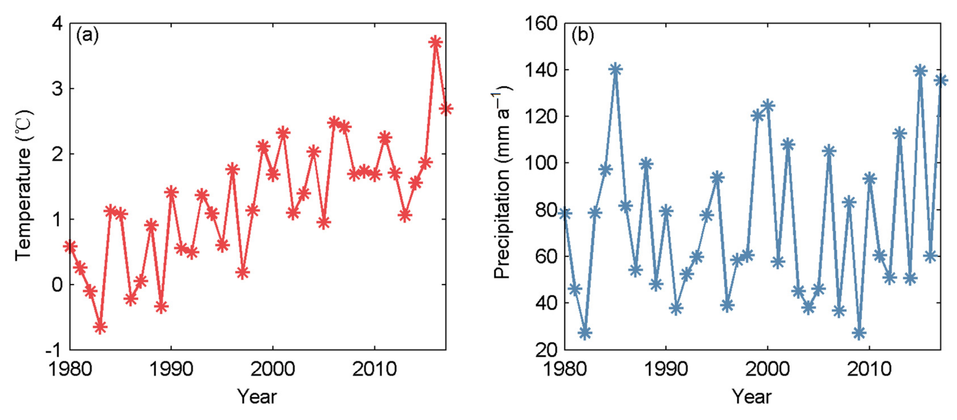
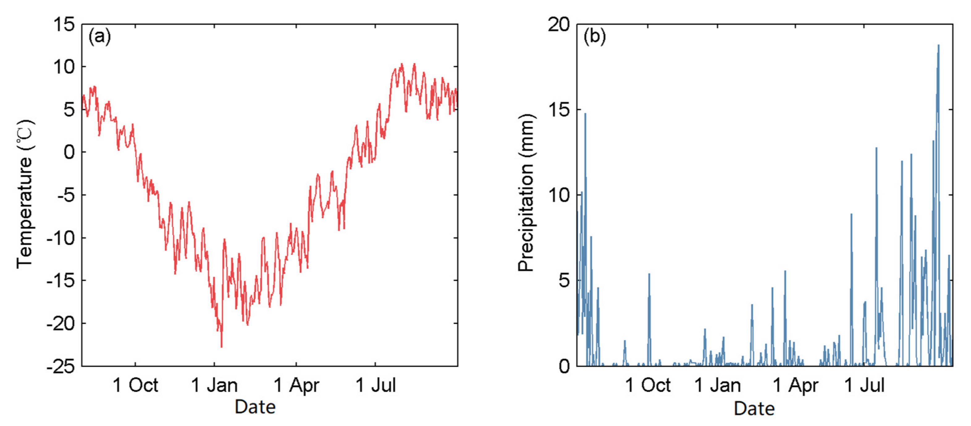
Data from the nearest meteorological station to the glacier, Shiquanhe (32.5° N, 80.08° E, 4279 m a.s.l., 85 km away from the glacier), show that, over the past three decades, the mean annual air temperature has increased by 0.063 °C a−1, while the annual precipitation shows no trend (Figure 2). There is an automatic weather station (AWS; 32.87° N, 80.92° E, 5640 m a.s.l; Figure 1) near the terminus of Da Anglong Glacier. Daily air temperatures and precipitation at the AWS were measured from 1 August 2015 to 25 August 2016 (Figure 3). The mean annual temperature lapse rate is 0.65 °C (100 m)−1 between the AWS and Shiquanhe station from August 2015 to July 2016. Daily temperatures at the AWS and Shiquanhe station are well correlated (r = 0.83) but daily precipitation less well (r = 0.45), as may be expected in mountainous regions. Precipitation is concentrated in summer on Da Anglong Glacier (Figure 3), meaning that both the main ablation and accumulation seasons are in summer, and temperatures at the AWS site are above the freezing point for around 5 months of the year.
Surface topography and bed elevation were measured by differential GPS and ground penetrating radar (GPR). SMB and ice velocity were estimated by repeated stake observations in August in 2014 and 2015 and October in 2016 and 2017. The differential GPS used was Starfire E3050 in 2014 and 2015 and Starfire E3040 in 2016 and 2017. The GPS vertical precision is 0.1 m and the horizontal precision is 0.05 m. There is a supraglacial stream on the surface of the glacier flowing roughly along the center flow line, limiting surveys to only one side of the river (Figure 4). Elevations above 6150 m were not surveyed due to terrain hazards. Ice thickness was measured in 2016 by Pulse Ekko 100 GPR with antenna center frequency of 100 MHz, with a 4 m antenna spacing and measurement interval. The ice thickness data has an accuracy of 1–2 m. The maximum thickness measured was 216 m.
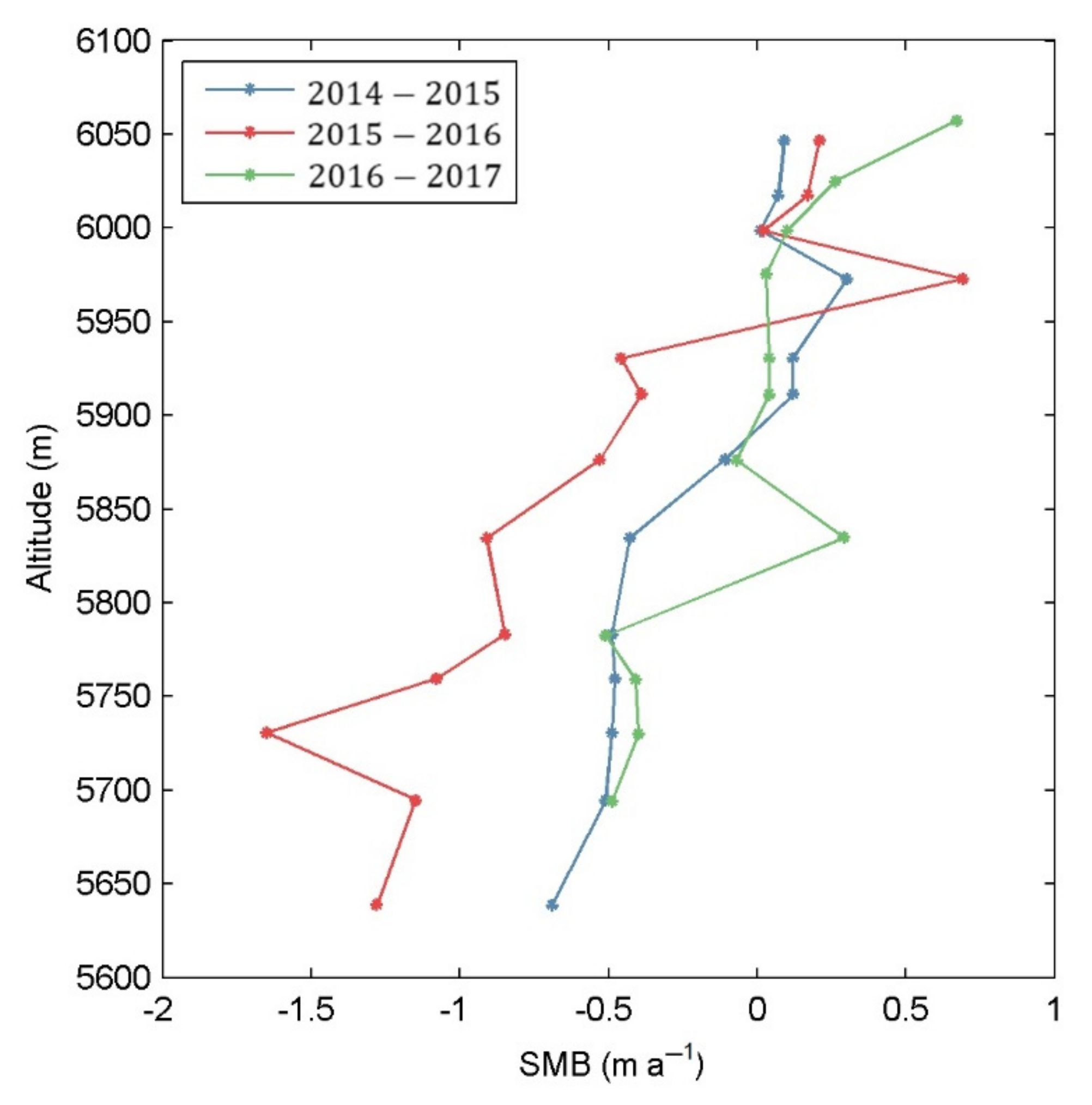
Figure 5 shows the measured SMB-elevation profile from the stakes on the glacier between 2014 and 2017. SMB was measured over the elevation range 5600–6100 m, and the Equilibrium Line Altitude (ELA) was at 5900–5950 m. The mean annual surface velocity measured at the stakes was 4.4 m a−1, with the maximum of 6.0 m a−1 at 5834 m elevation. We also analyzed satellite velocity data at 240 m spatial resolution, generated using auto-RIFT [20] and provided by the NASA MEaSUREs ITS_LIVE project [21], to compare with field measurements. Annual velocities are provided at yearly intervals. The imagery used to create the velocity mosaics comes from USGS/NASA’s Landsat 8 Operational Land Imager-Band 8 (15 m resolution).
3. Surface Mass Balance Parameterization
We have SMB measurements (Figure 5) in three different mass balance years: from August 2014 to August 2015, from August 2015 to October 2016, and from October 2016 to October 2017. We parameterize glacier accumulation and ablation as a function of local temperature and precipitation based on the measurements at the AWS and Shiquanhe station.
3.1. Accumulation
Da Anglong Glacier is located at the upper reaches of the Indus River, which is influenced by westerly air flow and precipitation sources. Sun et al. [22] found that precipitation firstly increases to a maximum and then decreases with elevation in the basins influenced by westerlies over the Tibetan Plateau. They also estimate the average annual precipitation gradient in the upper Indus basin, 0.29 mm m−1, which equals a daily mean precipitation gradient of 0.08 mm (100 m)−1. We calculated the daily precipitation gradients using the observed daily precipitation at the AWS near the glacier and Shiquanhe station, from August 2015 to August 2016. We found that the daily precipitation gradients are concentrated between 0.1 mm (100 m)−1 and 0.2 mm (100 m)−1, see Figure 6, which is close to the above finding in [22], considering the natural variability within mountainous regions.
The precipitation gradient in reality varies with elevation. The profile of precipitation firstly increasing then decreasing with elevation in the basins influenced by westerly winds [22] implies that the precipitation gradient changes from positive to negative at the maximum precipitation height. We use a quadratic polynomial to capture this feature of precipitation gradient. Three pairs (elevation, precipitation gradient) fully determine the quadratic polynomial. We choose three elevations, the AWS, Shiquanhe station, and the maximum precipitation height. The observed SMB in both the years 2014/2015 and 2015/2016 reaches a maximum at 5975 m (Figure 5), which take to mean that the precipitation reaches a local maximum near that elevation. Therefore, we assume the daily precipitation gradient is zero at 5975 m.
Because the daily precipitation gradients are mostly in the range of 0.1–0.2 mm (100 m)−1, we explore daily precipitation gradients at the Shiquanhe station and AWS by selecting from the set {0.1, 0.15, 0.2} mm (100 m)−1, giving nine combinations of daily precipitation gradients at the Shiquanhe station and the AWS. Having fixed the zero of precipitation gradient at 5975 m, we fit a quadratic polynomial to the daily precipitation gradients (Figure 7a), then integrate it from 4278 m to all the elevations on the glacier surface and estimate precipitation there (Figure 7b).
The quadratic polynomials using the above nine combinations give total precipitation at the elevation of the AWS from August 2015 to August 2016 in the range of 961–1860 mm. The quadratic polynomial with daily precipitation gradient value of 0.1 mm (100 m)−1 day−1 at the Shiquanhe station and 0.15 mm (100 m)−1 day−1 at the AWS gives a total precipitation value of 1303.7 mm, closest to the observed 1302.7 mm, at the AWS over the same period. Therefore, we use the best-fit quadratic polynomials of daily precipitation gradients (Figure 7a) hereafter.
Next, we calculated (elevation-dependent) daily solid precipitation, , as follows [23]:
where P represents daily total precipitation and T, daily mean temperature. and are the critical values for liquid and solid precipitation, taken as 0 °C and 4 °C, respectively. Elevation-dependent glacier accumulation is obtained by summing daily solid precipitation.
3.2. Ablation
We employ the widely used (e.g., [24]) positive degree-day model [25] to estimate the ablation at different elevations. The annual ablation rate is calculated by multiplying the sum of positive daily mean air temperatures (PDD) by a suitable degree-day factor (DDF) as follows:
is daily temperature. is logical function, set to 1 when and else 0.
The DDF determines the amount of ice and snow ablation produced by unit positive accumulated temperature. The choice of DDF greatly affects the accuracy of the model. DDF ranged from 2.6 to 13.8 mm∙d−1∙°C−1 on 15 glaciers across the Tibetan Plateau [24], increasing from northwest to southeast. Maritime (that is, comparatively warm and wet) glaciers have higher DDF than subcontinental and extremely continental glaciers, which may be characterized as cold and dry. Deng and Zhang [26] studied degree–day factors from 24 glaciers on the Tibetan Plateau, and also found a tendency for high values in the east and south and low values in the west and north.
We estimate daily precipitation on the glacier for the three mass balance periods (2014/2015, 2015/2016, 2016/2017) using daily precipitation records at the Shiquanhe station and the estimated best-fit precipitation gradient (Section 3.1).
We estimate the SMB using solid precipitations in Equation (1) and ablation calculated in Equation (2), with the DDF selected from the range of [2.6, 13.8] mm∙d−1∙°C−1 to minimize misfit with observed SMB (Figure 5) in three mass balance periods. We find a DDF of 3.4 mm∙d−1∙°C−1 gives the best fit (Figure 8) and is reasonable for glaciers in the region [24].
These best SMB parameters are used to parametrize SMB for future simulations. Additionally, we impose a limit on the maximum SMB on the glacier of 0.5 m since observed SMB rarely exceeds 0.5 m even at the highest point of the glacier (Figure 5) due to frequent strong winds. Furthermore, the upper glacier surface and the side walls that constrain it are almost the same elevation, suggesting that the highest elevation parts of the glacier are close to, or at, maximum possible elevation.
4. Ice Flow Modeling
Da Anglong Glacier flow dynamics were modeled using the thermo-mechanically coupled full-Stokes model, Elmer/Ice, an open source finite element code that has been used to simulate several mountain glacier flow models successfully [16,27,28].
4.1. Field Equations
Elmer/Ice is a thermo-mechanically coupled full-Stokes model that includes the following equations:
Ice density, , is set to 910 km·m−3. is the vector of ice flow velocity. Equation (5) expresses the conservation of momentum, where is the deviatoric stress tensor, is the isotropic pressure, and g is the acceleration due to gravity (0,0,−9.81) m·s−2. Via Glen’s flow law, the deviatoric stress tensor is related to the deviatoric part of the strain rate tensor, D, which can be described by
where denotes ice viscosity, given by
where the flow rate factor A(T) is derived from an Arrhenius law [29]; de is the second invariant of the strain-rate, (0.5trD2)1/2, and the Glen exponent n is taken as 3. Equation (6) is the heat transfer equation, and T is ice temperature. The heat capacity c and heat conductivity K are functions of ice temperature [29]. The ice temperature is bounded by an upper limit at the pressure melting point.
4.2. Boundary Conditions
Da Anglong Glacier is entirely above 5000 m elevation, so we initially assumed that the bottom of the glacier is frozen and non-sliding. The radargram along the flowline shows a consistent ice-bedrock interface that does not suggest any of the glacier is subject to basal melt [19], though that does not mean that basal melt is certainly excluded. We set a Neumann boundary condition at the ice bottom interface for temperature simulation with a geothermal heat flux. Jiang et al. [17] compiled geothermal heat flux data for China; there are no geothermal heat flux measurements in this region, and data are very sparse on the western Tibetan Plateau. Their map shows the glacier is located on a transition region between the Central China Orogen with low-medium heat fluxes and the Tibet-Saijiang Orogen with higher fluxes, and probably has a heat flux in the range 50–60 mW m−2. Therefore, we tested values of 50 and 60 mW m−2 for geothermal heat flux and determine a likely value based on comparison between modeled and observed surface flow velocity (Section 5).
We prescribe a stress-free condition at the glacier surface, meaning that atmospheric pressure and its change over the glacier surface are neglected. Surface temperature is estimated by annual mean temperature and a lapse rate of 0.65 °C (100 m)−1.−7.1 °C is the annual mean temperature from the Shiquanhe station:
where T is the glacier surface temperature (°C) and z is surface elevation (m a.s.l.).
The evolution of the free surface in prognostic simulations was modeled by a kinematic boundary condition:
where z is surface elevation; u, v and w denote ice flow velocity components in the x, y, and z direction, respectively; SMB is calculated as described in the SMB parameterization section.
4.3. Climate Forcing Scenarios
For the period 2016–2098, we estimated the time series of SMB by the method in Section 3 based on output from the 25-km-resolution regional climate model RegCM4 ([30], available online: https://esgf-data.dkrz.de/search/cordex-dkrz/ (accessed on 11 November 2021)). RegCM4 was nested within three different Earth System Models (ESMs): HadGEM2−ES [31], MPI−ESM−MR [32], and NorESM1−M [33], all running the RCP2.6 and RCP8.5 scenarios.
The mean annual air temperature increases at the AWS during the 21st century range from 0.002–0.008 °C a−1 under RCP2.6 to 0.054–0.068 °C a−1 under RCP8.5 (Figure 9a, Table 1). HadGEM2ES projects the largest rise while MPI−ESM−MR, the lowest. The ensemble mean projected rise rates are 0.006 °C a−1 under RCP 2.6 and 0.059 °C a−1 under RCP 8.5. We bias correct RegCM4 modeled daily temperatures using observed temperatures over 1980–2005 at the Shiquanhe station, with an altitudinal temperature lapse rate of 0.65 °C (100 m)−1 and correct monthly means with an offset from the 1980–2005 observations. Summer mean temperature dominates the glacier ablation in the whole year. The summer temperature rises slightly slower than mean annual temperature (Table 1). Again, HadGEM2ES projects the highest summer temperature rises.
The RegCM4 modeled daily precipitation at the nearest grid point to the AWS (within about 1 km) has a similar distribution to observations during its measurement period, and, since there is only 1 year of data, we do not bias correct modeled daily precipitation. There is no trend in modeled precipitation by all models under RCP 2.6 but a slightly increasing trend after the year 2050 under RCP8.5. The ensemble mean projected precipitation at the elevation of AWS is in the range of 831–1116 mm a−1 under RCP 2.6 and 778–1202 mm a−1 under RCP 8.5.
5. Glacier Geometry in the Year 2016
We produce the best-fit state of the glacier in the year 2016 from the detailed but spatially limited in situ observations, extended by inverse modeling of the glacier velocities to estimate errors in ice thickness based on the spatially complete but bias-prone Shuttle Radar Topography Mission (SRTM version 4.1 with resolution of 90 m) dataset measured in the year 2000.
The SRTM dataset specifies 90% of errors will be <16 m [34]. Since this error is not random either spatially or temporally, we must consider the possibility of a bias in the SRTM data. The glacier surface profile in 2000 would have been different from 2016 because of trends in SMB. These will not be uniform over the glacier: in a warming climate, the lower glacier will thin more than the upper parts. In contrast with this actual change in glacier geometry, a bias in SRTM data will produce an offset to elevations, for example, due to local errors in representing the geoid.
The surface elevation data measured by GPS in the year 2016 are about 30 m lower than those from the year 2000 SRTM dataset at the corresponding locations, with no trend with elevation, suggesting that a bias rather than an SMB signal dominates this offset. Therefore, we lower the surface elevation from SRTM dataset by 30 m everywhere to get a glacier surface elevation map in the year 2016 (Figure 10a). This 30 m includes both the error in the SRTM dataset and the elevation change from the year 2000 to 2016. If, instead of allowing this correction to the SRTM data, we assumed the SRTM elevations were correct, it would imply a surface lowering of 30 m between 2000 and 2016 and a mean lowering rate far in excess of any remote sensing observations in the region [35]. Shean et al. [35] generated a 30 km resolution elevation change trend map from 2000 to 2018 and found an estimated local mean mass balance of −0.2 ± 0.2 m a−1 in the hexagonal cell containing Da Anglong Glacier. Observed surface lowering rates below the ELA (0–0.6 m a−1) corresponds to 0–10 m surface lowering between 2000 and 2016. Furthermore, simulations with the SRTM geometry do not lead to terminus retreat as observed [19]. Therefore, the SRTM data is likely to overestimate the surface by 20–30 m in the lower part of Da Anglong Glacier, which is more than estimated 90th percentile of SRTM errors.
Next, we estimate the ice thickness in the year 2016. We measured ice thickness using GPR along several routes in 2015/2017 (Figure 4). However, the measurements are spatially limited and absent in the upper glacier. To get better spatial coverage of ice thickness, we supplement them with the modeled ice thickness for Da Anglong from the inverse model GlabTop2 [36]. GlabTop2 uses SRTM surface elevation data and empirical thickness–slope relations, a semi-elliptic cross-sectional geometry, and an estimate of basal shear stress from glacier vertical extent. GlabTop2 underestimates the mean ice thickness by 7% at six glaciers surveyed by radar measurements, but it also tends to overestimate small ice thicknesses [36]. Therefore, we cannot simply take GlabTop2 ice thicknesses as correct for the year 2016.
We do, however, have an ice dynamics model that can be used to give surface velocities for arbitrary glacier geometries. Hence, we can refine the ice thickness by manually doing an inversion process using the ice flow model to minimize misfit between modeled ice velocity and that measured by the GPS survey of the stakes on the glacier. For the upper part of the glacier, where radar data are absent, we take GlabTop2 ice thickness as an initial estimate and modify it to match the location of observed thickest ice. We manually generate thickness correction data based on the distances to the thickest part of the glacier, assuming the ice thickness in the lower glacier has high accuracy while the upper part has large uncertainty. These different ice thickness corrections are then used to produce simulations of surface velocity we can compare with the observations. We define a relative velocity error as
where N is number of observations, and are observed and modeled velocities at each stake. The end results are ice thickness (Figure 10c) and surface velocity maps that best-fit observed stake velocities. We find that a geothermal heat flux of 60 mW m−2 produces a 10–20% better fit than with lower heat flux. We produce a bed geometry map by subtracting the best-fit ice thickness estimates from the glacier surface elevation in the year 2016, correcting SRTM elevations by 30 m (Figure 10b). This bed elevation is well correlated (r = 0.9) with the GPR measurements we made in the years 2015/2017. The RSME between the estimated bed elevation and GPR measured is 5.7 m.
We compare observed, modeled, and remotely sensed velocities at the stake sites in Figure 11. The uncertainty of imagery-derived velocity is quoted at 0.3 m a−1 for this glacier [21]. Figure 11 shows that the imagery-derived velocities are generally much lower (with differences far greater than the nominal satellite errors) than those from stake observations or our model, which is not entirely unexpected as Da Anglong Glacier is a relatively slow flowing (<10 m a−1) glacier. Millan et al. [37] found that capturing fluctuations below 10 m a−1 remain challenging even for Sentinel-2, which they found is about twice as precise as that from Landsat 7/8 on some mountain glaciers. There are smaller errors between the stake and modeled velocities than between stake and satellite-derived velocities, showing that the image data is not especially helpful in extending the stake velocity observations, and, indeed, the remotely sensed velocities are so low as to be unphysical for an ice body of this observed thickness. Observed velocities are slightly larger than simulated, indicating that some sliding is occurring in addition to the pure ice deformation that we prescribed by specifying the no-slip condition at the bed.
6. Model Projections from 2016 to 2098
Using the geometry for the year 2016, we build a 3D ice dynamic model with unstructured triangular elements at 50 m spatial resolution with 16 terrain-following layers between the bedrock and surface. We applied both diagnostic and prognostic simulations. The former was done for a fixed geometry in the year 2016, with the purpose of building the steady-state temperature and velocity fields, and then to use it as an initial condition for prognostic simulations during the period 2017–2098. Simulations were done using geothermal heat fluxes of 50 and 60 mW m−2.
We assumed that the glacier is not sliding on its bed, and the resulting basal temperature map (Figure 12) in the year 2016 is below pressure melting point by more than 2.2 °C everywhere for 50 mW m−2 and by 0.6 °C for 60 mW m−2 heat fluxes. Although this temperature field is consistent with no sliding, water can be present beneath a glacier at lower temperatures [38]. Furthermore, this is a steady state simulation, whereas we have argued that the glacier has been thinning at least over the 21st century. A thicker glacier in the 20th century may have had areas at the pressure melting point. This would lead to faster sliding velocities. We consider the result to be compatible with the limited sliding suggested by velocities in Figure 11. The modeled maximum ice velocities in the year 2016 are 5.6 m a−1 and 6.3 m a−1 with geothermal heat fluxes of 50 and 60 mW m−2, respectively (Figure 13).
The prognostic simulation from 2016 to 2098 was forced by projected temperatures and precipitations from RegCM4 driven by the three ESMs under the RCP2.6 and RCP8.5 scenarios (Section 4.3) with geothermal heat fluxes of 50 and 60 mW m−2. While basal heat flux makes significant changes to surface velocities (Figure 11), it has little impact on glacier volume and area evolution.
Simulated glacier volume loss during 2016–2098 is equivalent to 16–62% of the glacier volume in the year 2016 under RCP2.6 and 75–91% under RCP8.5 (Figure 14). Therefore, the average annual volume loss rate is 0.19–0.75% a−1 under RCP2.6 and 1.0–1.1% a−1 under RCP8.5. Ensemble mean volume loss rate during 2016–2098 is 0.46% a−1 of the glacier volume in the year 2016 under RCP2.6 and 1.0% a−1 under RCP8.5.
Summer mean temperature dominates glacier ablation. RegCM4 forced by HadGEM2ES projects the highest summer mean temperature among the ensemble and, thus, the largest volume loss, while RegCM4 forced by MPI−ESM−MR projects the lowest. Simulated glacier area loss during 2016–2098 is equivalent to 11–39% of the glacier area in the year 2016 under RCP2.6 and 60–83% under RCP8.5 (Figure 15). Therefore, the annual averaged area loss rate across ESMs is 0.13–0.47% a−1 under RCP2.6 and 0.72–1.00% a−1 under RCP8.5. Ensemble mean area loss rate during 2016–2098 is 0.22% a−1 of the glacier area in the year 2016 under RCP2.6 and 0.87% a−1 under RCP8.5.
We also compared simulated volume change in the final year 2098 from prognostic simulations with and without ice dynamics (Figure 14), and found relative difference of 24% (range 22–27%) under RCP2.6 and 20% (16–24%) under RCP8.5. Ice dynamics transports ice to the lower part of the glacier where more ablation occurs. Therefore, ice dynamics play a relatively larger role under RCP2.6 because surface temperature and ablation rate increases are lower than under RCP8.5. For small Tibetan glaciers like the Gurenhekou Glacier and Qiangtang No. 1 Glacier [13,16], SMB is the overwhelmingly dominant factor in mass loss. This is because the ice flow speed of glaciers scales strongly (theoretically, with the fourth power) of ice thickness and, thus, larger glaciers with greater mean thickness are much more dynamic than small glaciers. Changes to the dynamics of larger glaciers are relatively slow because the climate-driven changes in geometry that drive ice flow take longer to modify large glaciers and, thus, ice dynamics provide increasingly important positive feedback on larger glaciers in warming climates.
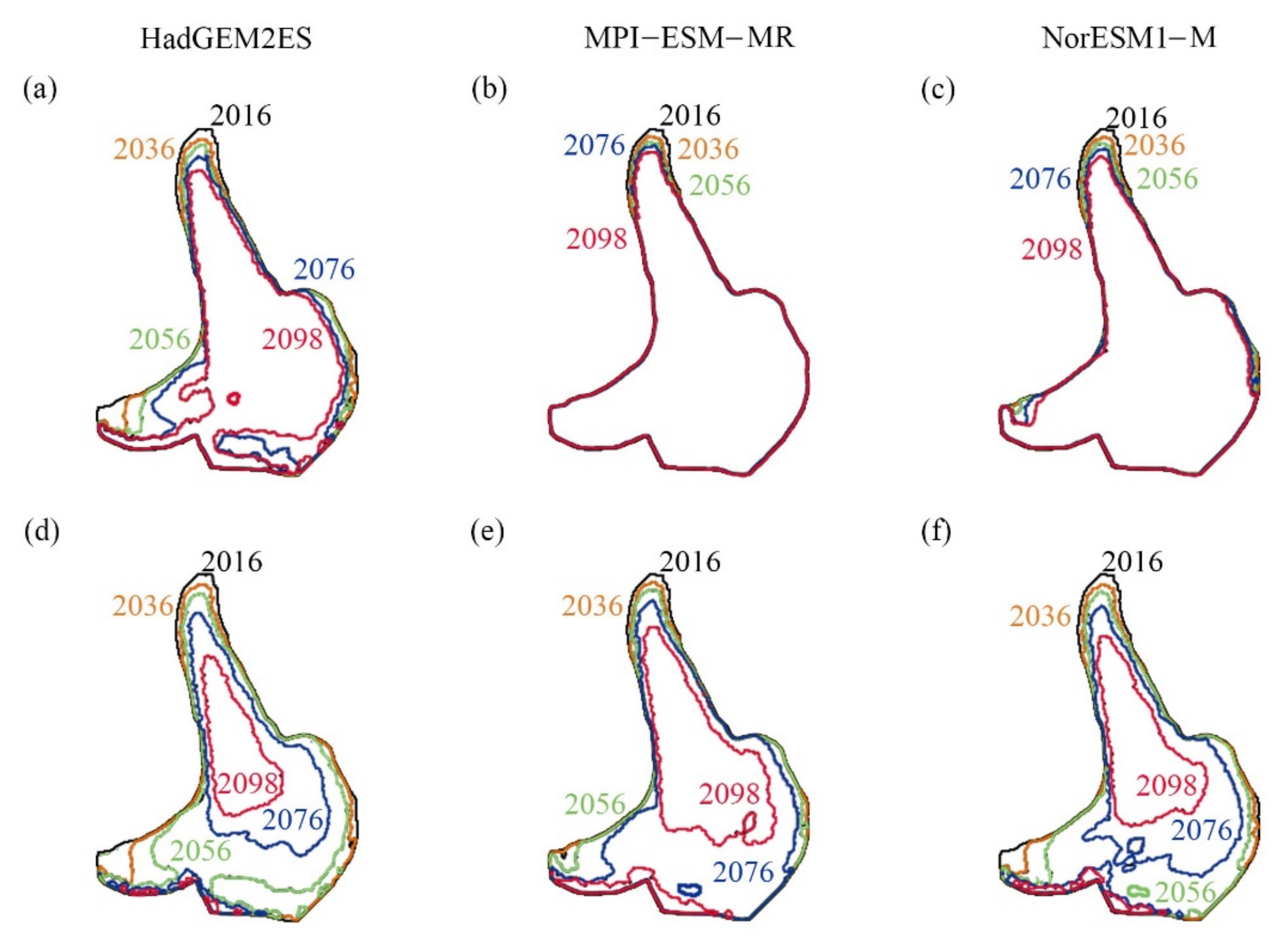
The measured annual mean terminus retreat rate from 2000 to 2015 is 5.2 m a−1 [19]. Modeled terminus retreats from 2016 to 2098 projected from RegCM4 displays differences between ESMs (Figure 15). Differences between models are much smaller than differences between scenarios, indicating the dominance of emissions scenario over ESM differences on the glacier evolution. Modeled glacier terminus retreat rate from 2016 to 2098 is 2.9–5.9 m a−1 under RCP2.6 and 7.7–12.5 m a−1 under RCP8.5. The simulated upper part of the glacier also shrinks under RCP8.5. The model suggests that only the central part of the glacier will exist by the end of this century under RCP8.5.
7. Discussion
The large relative difference in projected glacier volume changes when considering ice dynamics shows that both SMB and ice transport downslope are important factors in glacier evolution in the coming decades. This is different from previous studies on a few smaller glaciers on the Tibetan Plateau [13,16] where SMB is the only dominant factor. This finding shows that ice dynamics cannot be ignored in mass balance estimation for Tibetan glaciers, especially those large ones that dominate the sea level rise contribution.
Accurate modeling of ice dynamics requires knowledge of glacier geometry, which is derived from data on surface elevation and ice thickness. In the case of Da Anglong, it is difficult to measure ice thickness in the upper part of glacier due to the dangerous conditions. We only have observed surface elevation, ice thickness, and surface velocity at the lower part of the glacier. Ice thickness generation for large glaciers without full spatial coverage of measurements is challenging. We modify the SRTM dataset by 30 m to generate the glacier surface elevation in the year 2016 (Section 5). Applying this procedure gives a mean difference of 0.59 m from measured surface elevation with an RSME of 2.83 m. This seems reasonable given the seasonal fluctuations expected in glacier thickness. The 30 m correction, we argue, is plausible according to the stated uncertainties in SRTM data.
Various statistical models have been published that seek to estimate the ice thickness distribution of mountain glaciers from surface characteristics based on considerations of ice flow dynamics and mass conservation, including the 13 models that participated in the Ice Thickness Model Intercomparison eXperiment [39]. These are very useful where large numbers of glaciers allow for cancellation of random errors in volume but will not always produce adequate results for any single glacier. In this study, we developed a novel way to accommodate these data limitations by using an inverse procedure with the full-Stokes ice flow model generating surface velocities that can be compared with the observed surface velocity to deduce ice thickness in the un-surveyed upper glacier. Using the optimized ice thickness in the lower glacier, the estimated bed elevation is well correlated (r = 0.9) with the GPR measurements in the lower part of the glacier. The RSME between the estimated bed elevation and GPR measured is 5.7 m. The uncertainty from the radar data is expected to be 1–2 m, but there is an additional uncertainty due to positioning errors and the underlying roughness of the bed.
Velocity was only measured in the ablation zone of Da Anglong Glacier, where velocities are generally higher than those simulated, with an averaged relative error of 30–50% with geothermal heat flux of 50 mW m2 and 10–40% with 60 mW m2. The modeled underestimation might be because we simulate ice deformation alone, consistent with the assumption of no basal sliding and basal ice temperatures about 0.6 °C below the pressure melting point with the present-day ice thickness. The slightly faster velocities might be the result of melting at the base in the recent past when the glacier was thicker, and sliding over the bed would also generate frictional heat that could sustain a supply of lubricating water as the glacier cooled slowly by thinning. The absence of a complete surface velocity map of the glacier is one large limitation and uncertainty source on the modeled results. When and if an accurate map of surface velocity for the glacier becomes available, we can do an inversion for the basal friction coefficient in basal sliding law, resulting in a better fit between the modeled ice velocity and the observed.
An obvious source of surface velocities might be from remote sensing images. We also analyzed satellite velocity data at 240 m spatial resolution generated using auto-RIFT [20] and provided by the NASA MEaSUREs ITS_LIVE project [21] to compare with field measurements. Annual velocities are provided at yearly intervals. The imagery used to create the velocity mosaics comes from USGS/NASA’s Landsat 8 Operational Land Imager-Band 8 (15 m resolution). We compared observed stake velocities on the glacier and those derived from satellite images and find the images underestimate the stake observation velocities, with twice the misfit as for the modeled velocities and with errors much larger than estimated for the derived satellite velocities [21]. This contrasts with experience from other glaciers in HMA: Dehecq et al. [40] found satellite derived annual velocity compared well with measurements in 2003 [41] from the ablation area for the Chhota Shigri Glacier, in Himachal Pradesh. However, very few measurements of glacier velocity exist in HMA and the utility of satellite-derived annual velocity would probably benefit from more widespread field measurements. Gardner et al. [21] acknowledge that the formal errors they quote seem too low and suggest that they should be used rather as qualitative metrics for assessing error. This might be so, but, with few verifications of the satellite product, it is hard to know how to interpret the given error. The ice velocity on Da Anglong Glacier is only slightly higher than pure internal ice deformation expected from its geometry and, hence, is flowing at nearly the slowest rate possible, since any basal lubrication would increase surface velocities. The internal deformation rate of glaciers should provide a minimum bound on glacier speeds, and, with statistical methods of estimating ice volume from surface observations as discussed earlier, would perhaps be usefully included in large-scale multi-glacier velocity estimates.
Precipitation gradient and DDF are crucial parameters in the SMB estimation, but they have large spatial and temporal variability over Tibetan glaciers [22,24,42]. Due to lack of measurements, many previous studies use the simple assumption of a linear relationship between precipitation with elevation, but this assumption is rather different from the sparse observations in the region [22,43,44,45] and, thus, likely introduces systematic errors in mountainous regions. This motivated us to use a quadratic elevation-dependent precipitation gradient parameterization based on the actual observed precipitation and SMB measurements. The very limited data available do not justify a detailed analysis with Monte Carlo searching of parameter space, and, thus, we can only estimate gradients to the nearest 0.05 mm (100 m)−1 day−1. Although we accounted for spatial variability, the paucity of data also means we cannot consider temporal variability due to the short observational period. In a region where the influence of both westerlies and monsoonal precipitation can be expected, the changes in precipitation gradient over time may well be important. Furthermore, the possible impact of climate warming on the climatic setting of the glacier might change the gradients in the future. However, the DDF factor, we deduce, is consistent with the observed variation of DDF across the region. The DDF is at the low end of the range on the Tibetan Plateau, indicating continental conditions for the glacier, as might be expected from its location.
A future step in simulating SMB might be a more sophisticated surface energy and mass balance model [46,47,48] or application of an operational physical model such as WRF [49]. However, these models have challenging data requirements and require many climate fields as drivers and sources of validation. These observations are very rare on the Tibetan Plateau, and reanalysis products are typically in error by an order of magnitude in snow accumulation [50].
Geothermal heat flux is an important boundary condition for ice flow models. It is essential to determine the ice temperature and, hence, ice viscosity and ice flow velocity. To match modeled ice velocity with measurements, we compared modeled ice velocity under different geothermal heat flux with observation, finding better fits with a geothermal heat flux of 60 mW m−2 than 50 mW m−2. We experimented with heat fluxes as low as 30 mW m−2 and these produce ice velocities well below observed, and, conversely, higher heat fluxes that produce extensive regions of the glacier bed at the melting point lead to surface velocities much faster than observed. Thus, in this glacier, the ice velocity data provide a fairly strong constraint on geothermal heat flux—which, in a sparsely surveyed region, can provide a useful datum. However, the heat flux makes only a negligible difference to ice volume loss, despite the importance of ice dynamics for Da Anglong Glacier. Therefore, derivation of the geothermal heat flux from glaciological velocity observations requires both sufficient observations of surface velocity, and sufficient ice geometrical data to simulate a full-Stokes flow model. The procedure would not be feasible on typical small glaciers where ice dynamics are slower, and mass wastage rates due to SMB are relatively larger than on the exceptionally large Da Anglong Glacier.
One way of testing the glacier dynamics model is to compare the modeled surface lowering with observations. We do this with a simulation for the period 2001–2015 starting from the steady state results in the year 2000. Our averaged modeled surface elevation lowering rates from 2000 to 2015 is about 0.4 m a−1 over the whole glacier. This can be compared with estimates from satellite altimetry. Brun et al. [5] estimated glacier elevation change rate in HMA from the year 2000 to 2016 and found surface lowering of 0.7 m a−1 in Himalaya but increases in elevation of close to 0.2 m a−1 in western Kunlun and eastern Pamir, with a gap in data coverage over our region of interest, consistent with Shean et al. [35] estimates of −0.2 ± 0.2 m a−1. The quoted uncertainty is only the estimated standard deviation with a necessarily incomplete knowledge of unknown systematic biases. Therefore, we judge that this satellite derived lowering rate is not significantly different from our modeled results.
Simulated ensemble mean volume loss rate during 2016–2098 is 0.46% a−1 of the glacier volume in the year 2016 under RCP2.6 and 1.0% a−1 under RCP8.5. Both area and volume loss rates have wider across-ESM model spread under RCP2.6 than RCP8.5, for example, volume loss rates range 0.19–0.75% a−1 under RCP 2.6 and 0.91–1.1% a−1 under RCP8.5. This is due to the much larger warming under RCP8.5 with SMB relatively more important than ice dynamics.
Our ensemble mean mass loss in the region from the year 2016 to 2098 is 38% under RCP2.6 and 83% under RCP8.5. This estimate under RCP2.6 is close to the ensemble mean mass loss estimates for the subregion South Asia West from the year 2015 to 2100 of 35% by Marzeion et al. [15] and 42% by Hock et al. [14] from glacier models forced with General Circulation Models. The estimate under RCP8.5 is larger than the ensemble mean mass loss for the subregion South Asia West from the year 2015 to 2100 of 62% by Marzeion et al. [15] and 65% by Hock et al. [14]. However, their models give a very wide range of estimates: 48–80% by Marzeion et al. [15] and 42–83% by Hock et al. [14].
8. Conclusions
Suites of simulations for Da Anglong Glacier have been made for the period 2016–2098 based on SMB parameterizations with projected temperature and precipitation from the 25-km-resolution RegCM4 nested within three ESMs running the RCP2.6 and RCP8.5 scenarios. We parameterized SMB using the positive degree-day method. We fit quadratic polynomials for an elevation-dependent precipitation gradient, using daily precipitation gradients at different elevations estimated by measured precipitation at both a local AWS and a regional meteorological station. The key factor, DDF, in the degree-day model for Tibetan glaciers in literature is expected to lie within the range 2.6 to 13.8 mm∙d−1∙°C−1. The best-fit DDF to the field observations is 3.4 mm∙d−1∙°C−1 for Da Anglong Glacier, which is comfortably at the continental climate end of the range of glaciers and typical of the northwest Tibetan Plateau [24].
Da Anglong Glacier had an area of 6.92 km2 in the year 2000 and 6.66 km2 in 2016. Observations on the upper glacier are missing because of dangerous conditions. To deal with this, we developed a novel inverse procedure using GlabTop2 output as the initial ice thickness and the full-Stokes Elmer flow model to determine ice velocities for a given map of ice thickness. We modified ice thickness to minimize misfit between modeled steady-state surface velocity and the measured surface velocity.
By using field observations within the ice dynamics model, we showed that Da Anglong Glacier ice thickness is beyond the 90th percentile of uncertainty in SRTM elevation data in the year 2000. SRTM ice elevations imply a glacier too thick to undergo its documented terminus retreat. Furthermore, NASA MEaSUREs ITS_LIVE satellite velocity data are unphysically slow for a glacier as thick and steep as ground-based data show it to be. Hence, the remotely sensed data suggest simultaneously thicker and thinner ice than are observed from ground measurements on the glacier.
The modeled glacier loses 16–62% (ensemble mean of 38%) of its 2016 volume during 2016–2098 under the aggressive mitigation RCP2.6 scenario and 75–91% (ensemble mean of 83%) under the “business-as-usual” RCP8.5 scenario. The Paris 2015 agreement on greenhouse gas emissions produces a climate intermediate between these two extremes, thus we might expect Da Anglong to lose ½ to ¾ of its mass by 2100 under the existing greenhouse gas emissions agreement.
Simulation from 2016 to 2098 neglecting ice dynamics show an underestimation of 23–29% under RCP2.6 and 19–26% under RCP8.5 compared with including ice dynamics. This is different from the result found for small Tibetan glaciers [13,16] for which SMB is the only significant factor in mass loss. Thus, mass loss estimates for large glaciers, which dominate the total sea level rise commitment, may need to be estimated individually when evaluating large scale mass balance estimation for High Mountain Asia.
Author Contributions
Conceptualization, L.Z. and J.C.M.; methodology, L.Z. and W.Z.; software, W.Z. and L.Z.; validation, L.Z., W.Z. and J.C.M.; formal analysis, W.Z. and L.Z.; investigation, L.Z.; resources, L.Z.; data curation, L.T., W.Z., L.Z.; writing—original draft preparation, W.Z., L.Z.; writing—review and editing, L.Z., J.C.M., M.W., L.T.; visualization, W.Z.; supervision, L.Z. and J.C.M.; project administration, L.Z.; funding acquisition, L.Z., L.T. All authors have read and agreed to the published version of the manuscript.
Funding
This research was funded by the National Key Research and Development Program of China (2021YFB3900105) and the National Natural Science Foundation of China (No. 41941006, 41530748).
Institutional Review Board Statement
Not applicable.
Informed Consent Statement
Not applicable.
Data Availability Statement
The SRTM version 4.1 dataset was obtained from https://cgiarcsi.community/data/srtm-90m-digital-elevation-database-v4-1/ (accessed on 11 November 2021). The output of regional climate model RegCM4 was obtained from https://esgf-data.dkrz.de/search/cordex-dkrz/ (accessed on 11 November 2021). The historical temperature and precipitation data at Shiquanhe meteorological station was downloaded from http://data.cma.cn/ (accessed on 11 November 2021). The ice thickness determined using GlabTop2 model was downloaded from https://mountainhydrology.org/data-nature-2017/ (accessed on 11 November 2021). The in-situ observation data, Elmer/Ice model scripts and modelled results are available from the authors.
Acknowledgments
This study has been supported by the National Key Research and Development Program of China (2021YFB3900105) and the National Natural Science Foundation of China (No. 41941006, 41530748). We thank Gao Xuejie for providing the output of regional climate model RegCM4.
Conflicts of Interest
The authors declare no conflict of interest.
References
- Kang, S.; Xu, Y.; You, Q.; Flügel, W.-A.; Pepin, N.; Yao, T. Review of climate and cryospheric change in the Tibetan Plateau. Environ. Res. Lett. 2010, 5, 015101. [Google Scholar] [CrossRef]
- Pepin, N.; Bradley, R.S.; Diaz, H.F.; Baraer, M.; Caceres, E.B.; Forsythe, N.; Fowler, H.; Greenwood, G.; Hashmi, M.Z.; Liu, X.D.; et al. Elevation-dependent warming in mountain regions of the world. Nat. Clim. Chang. 2015, 5, 424–430. [Google Scholar]
- Zhu, X.; Wei, Z.; Dong, W.; Wen, X.; Liu, Y. Projected temperature and precipitation changes on the Tibetan Plateau: Results from dynamical downscaling and CCSM4. Theor. Appl. Climatol. 2019, 138, 861–875. [Google Scholar] [CrossRef]
- Azam, M.F.; Wagnon, P.; Berthier, E.; Vincent, C.; Fujita, K.; Kargel, J.S. Review of the status and mass changes of Himalayan-Karakoram glaciers. J. Glaciol. 2018, 64, 61–74. [Google Scholar] [CrossRef] [Green Version]
- Brun, F.; Berthier, E.; Wagnon, P.; Kaab, A.; Treichler, D. A spatially resolved estimate of high mountain Asia glacier mass balances, 2000–2016. Nat. Geosci. 2017, 10, 668–673. [Google Scholar] [CrossRef] [PubMed]
- Yao, T.; Thompson, L.; Yang, W. Different glacier status with atmospheric circulations in Tibetan Plateau and surroundings. Nat. Clim. Chang. 2012, 2, 663–667. [Google Scholar] [CrossRef]
- Nakićenović, N.; Sward, R. Special Report on Emission Scenarios; Cambridge University Press: Cambridge, UK, 2000; pp. 570–599. [Google Scholar]
- Marzeion, B.; Jarosch, A.H.; Hofer, M. Past and future sea level change from the surface mass balance of glaciers. Cryosphere 2012, 6, 1295–1322. [Google Scholar] [CrossRef] [Green Version]
- Radic, V.; Bliss, A.; Beedlow, C.A.; Hock, R.; Miles, E.; Cogley, J.G.. Regional and global projections of the 21st century glacier mass changes in response to climate scenarios from GCMs. Clim. Dyn. 2014, 42, 37–58. [Google Scholar] [CrossRef]
- Zhao, L.; Ding, R.; Moore, J.C. The High Mountain Asia glacier contribution to sea-level rise from 2000 to 2050. Annu. Glaciol. 2016, 57, 223–231. [Google Scholar] [CrossRef] [Green Version]
- Zhao, L.; Yang, Y.; Ji, D.; Moore, J.C. Glacier evolution in high mountain Asia under stratospheric sulfate aerosol injection geoengineering. Atmos. Chem. Phys. 2017, 17, 6547–6564. [Google Scholar] [CrossRef] [Green Version]
- Kraaijenbrink, P.D.A.; Bierkens, M.F.P.; Lutz, A.F.; Immerzeel, W.W. Impact of a global temperature rise of 1.5 degrees Celsius on Asia’s glaciers. Nature 2017, 549, 257–260. [Google Scholar] [CrossRef]
- Zhao, L.; Tian, L.; Zwinger, T.; Ding, R.; Zong, J.; Ye, Q.; Moore, J.C. Numerical simulations of Gurenhekou glacier on the Tibetan Plateau. J. Glaciol. 2014, 60, 71–82. [Google Scholar] [CrossRef] [Green Version]
- Hock, R.; Bliss, A.; Marzeion, B.; Giesen, R.H.; Hirabayashi, Y.; Huss, M.; Radić, V.; Slangen, A.B.A. GlacierMIP—A model intercomparison of global-scale glacier mass-balance models and projections. J. Glaciol. 2019, 65, 453–467. [Google Scholar] [CrossRef] [Green Version]
- Marzeion, B.; Hock, R.; Anderson, B.; Bliss, A.; Champollion, N.; Fujita, K.; Huss, M.; Immerzeel, W.W.; Zekollari, H. Partitioning the uncertainty of ensemble projections of global glacier mass change. Earth’s Future 2020, 8, e2019EF001470. [Google Scholar] [CrossRef] [Green Version]
- Li, Y.; Tian, L.; Yang, Y.; John, C.M.; Sun, S.; Zhao, L. Simulating the evolution of Qiangtang No. 1 Glacier in the central Tibetan Plateau to 2050. Arct. Antarct. Alp. Res. 2017, 49, 1–12. [Google Scholar] [CrossRef] [Green Version]
- Jiang, G.; Hu, S.; Shi, Y.; Zhang, C.; Wang, Z.; Hu, D. Terrestrial heat flow of continental China: Updated dataset and tectonic implications. Tectonophysics 2019, 753, 36–48. [Google Scholar] [CrossRef]
- Guo, W.; Liu, S.; Xu, J.; Wu, L.; Shangguan, D.; Yao, X.; Wei, J.; Bao, W.; Yu, P.; Liu, Q.; et al. The second Chinese glacier inventory: Data, methods and results. J. Glaciol. 2015, 61, 357–372. [Google Scholar] [CrossRef] [Green Version]
- Chen, Y.; Tian, L.; Zong, J.; Zhu, D.; Wang, C.; Jin, S. Variation of the large and small Anglong Glaciers in the Ali district, Tibet autonomous region. J. Glaciol. Geocryol. 2019, 41, 14–23, (In Chinese with English Summary). [Google Scholar] [CrossRef]
- Gardner, A.S.; Mohold, G.; Scambos, T.; Fahnstock, M.; Ligtenberg, S.; Van Den, B.M.; Nilsson, J. Increased West Antarctic and unchanged East Antarctic ice discharge over the last 7 years. Cryosphere 2018, 12, 521–547. [Google Scholar] [CrossRef] [Green Version]
- Gardner, A.S.; Fahnestock, M.A.; Scambos, T.A. ITS_LIVE Regional Glacier and Ice Sheet Surface Velocities. Data Archived at National Snow and Ice Data Center; 2019. Available online: https://its-live.jpl.nasa.gov/ (accessed on 15 January 2020).
- Sun, H.; Su, J.; Huang, J.; Yao, T.; Luo, Y.; Chen, D. Contrasting precipitation gradient characteristics between westerlies and monsoon dominated upstream river basins in the Third Pole. Chin. Sci. Bull. 2020, 65, 91–104. [Google Scholar] [CrossRef]
- Sakai, A.; Nuimural, T.; Fujita, K.; Takenaka, S.; Nagail, H.; Lamsal, D. Climate regime of asian glaciers revealed by gamdam glacier inventory. Cryosphere 2015, 9, 865–880. [Google Scholar] [CrossRef] [Green Version]
- Zhang, Y.; Liu, S.; Ding, Y. Spatial variation of degree-day factors on the observed glaciers in Western China. Acta Geogr. Sinica 2006, 61, 89–98. [Google Scholar] [CrossRef] [Green Version]
- Braithwaite, R.J. Calculation of degree-days for glacier–climate research. Z. Gletsch. Glazialgeol. 1984, 20, 1–20. [Google Scholar]
- Deng, C.; Zhang, W. Spatial distribution pattern of degree–day factors of glaciers on the Qinghai–Tibetan Plateau. Environ. Monit. Assess. 2018, 190, 475. [Google Scholar] [CrossRef]
- Adhikari, S.; Marshall, S.J. Influence of high-order mechanics on simulation of glacier response to climate change: Insights from Haig Glacier, Canadian Rocky Mountains. Cryosphere 2013, 7, 1527–1541. [Google Scholar] [CrossRef] [Green Version]
- Gagliardini, O.; Zwinger, T.; Gillet-Chaulet, F.; Durand, G. Capabilities and performance of elmer/ice, a new generation ice-sheet model. Geosci. Model Dev. 2013, 6, 1299–1318. [Google Scholar] [CrossRef] [Green Version]
- Paterson, W.S.B. The Physics of Glaciers, 3rd ed.; Elsevier: Oxford, UK, 1994. [Google Scholar]
- Gao, X.J.; Wu, J.; Shi, Y.; Wu, J.; Han, Z.Y.; Zhang, D.F.; Tong, Y.; Li, R.K.; Xu, Y.; Giorgi, F. Future changes in thermal comfort conditions over China based on multi-RegCM4 simulations. Atmos. Ocean. Sci. Lett. 2018, 11, 291–299. [Google Scholar] [CrossRef] [Green Version]
- Martin, G.M.; Ringer, M.A.; Pope, V.D.; Jones, A.; Dearden, C.; Hinton, T.J. The physical properties of the atmosphere in the new Hadley Centre Global Environmental Model (HadGEM1). Part I: Model description and global climatology. J. Clim. 2006, 19, 1274–1301. [Google Scholar] [CrossRef]
- Marsland, S.J.; Haak, H.; Jungclaus, J.H.; Latif, M.; Röske, F. The Max-Planck-Institute global ocean/sea ice model with orthogonal curvilinear coordinates. Ocean Model. 2003, 5, 91–127. [Google Scholar] [CrossRef] [Green Version]
- Bentsen, M.; Bethke, I.; Debernard, J.B.; Iversen, T.; Kirkevåg, A.; Seland, Ø; Drange, H.; Roelandt, C.; Seierstad, I.A.; Hoose, C.; et al. The Norwegian Earth System Model, NorESM1-M—Part 1: Description and basic evaluation of the physical climate. Geosci. Model Dev. 2013, 6, 687–720. [Google Scholar] [CrossRef] [Green Version]
- Falorni, G.; Teles, V.; Vivoni, E.R.; Bras, R.L.; Amaratunga, K.S. Analysis and characterization of the vertical accuracy of digital elevation models from the Shuttle Radar Topography Mission. J. Geophys. Res. 2005, 110, F02005. [Google Scholar] [CrossRef]
- Shean, D.E.; Bhushan, S.; Montesano, P.; Rounce, D.R.; Arendt, A.; Osmanoglu, B. A systematic, regional assessment of high mountain Asia glacier mass balance. Front. Earth Sci. 2020, 7, 363. [Google Scholar] [CrossRef] [Green Version]
- Frey, H.; Machguth, H.; Huss, M.; Huggel, C.; Bajracharya, S.; Bolch, T.; Kulkarni, A.; Linsbauer, A.; Salzmann, N.; Stoffel, M. Estimating the volume of glaciers in the Himalayan–Karakoram region using different methods. Cryosphere 2014, 8, 2313–2333. [Google Scholar] [CrossRef] [Green Version]
- Millan, R.; Mouginot, J.; Rabatel, A.; Jeong, S.; Cusicanqui, D.; Derkacheva, A.; Chekki, M. Mapping surface flow velocity of glaciers at regional scale using a multiple sensors approach. Remote Sens. 2019, 11, 2498. [Google Scholar] [CrossRef] [Green Version]
- Dash, J.G.; Rempel, A.W.; Wettlaufer, J.S. The physics of premelted ice and its geophysical consequences. Rev. Mod. Phys. 2006, 78, 695–741. [Google Scholar] [CrossRef] [Green Version]
- Farinotti, D.; Brinkerhoff, D.J.; Fürst, J.J.; Gantayat, P.; Gillet-Chaulet, F.; Huss, M.; Leclercq, P.W.; Maurer, H.; Morlighem, M.; Pandit, A.; et al. Results from the Ice Thickness Models Intercomparison eXperiment phase 2 (ITMIX2). Front. Earth Sci. 2021, 8, 571923. [Google Scholar] [CrossRef]
- Gourmelen, N.; Gardner, A.S.; Brun, F.; Goldberg, D.; Nienow, P.W..; Berthier, E.; Vincent, C.; Wagnon, P.; Trouvé, E.; Gourmelen, N. Twenty-first century glacier slowdown driven by mass loss in High Mountain Asia. Nat. Geosci. 2019, 12, 22–27. [Google Scholar] [CrossRef]
- Azam, M.F.; Wagnon, P.; Berthier, E.; Vincent, C.; Fujita, K.; Kargel, J.S. From balance to imbalance: A shift in the dynamic behaviour of Chhota Shigri glacier, western Himalaya, India. J. Glaciol. 2012, 58, 315–324. [Google Scholar] [CrossRef] [Green Version]
- Singh, V.; Goyal, M.K. Analysis and trends of precipitation lapse rate and extreme indices over north Sikkim eastern Himalayas under CMIP5ESM-2M RCPs experiments. Atmos. Res. 2016, 167, 34–60. [Google Scholar] [CrossRef]
- Yang, K.; Guyennon, N.; Ouyang, L.; Tian, L.; Tartari, G.; Salerno, F. Impact of summer monsoon on the elevation-dependence of meteorological variables in the south of central Himalaya. Int. J. Climatol. 2018, 38, 1748–1759. [Google Scholar] [CrossRef]
- Sevruk, B.; Mieglitz, K. The effect of topography, season and weather situation on daily precipitation gradients in 60 Swiss valleys. Water Sci. Technol. 2002, 45, 41–48. [Google Scholar] [CrossRef] [PubMed]
- Sevruk, B. Regional dependency of precipitation-altitude relationship in the Swiss Alps. Clim. Chang. 1997, 36, 355–369. [Google Scholar] [CrossRef]
- Klok, E.J.; Oerlemans, J. Model study of the spatial distribution of the energy and mass balance of Morteratschgletscher, Switzerland. J. Glaciol. 2002, 48, 505–518. [Google Scholar] [CrossRef] [Green Version]
- Jiang, X.; Wang, N.; He, J.; Wu, X.; Song, J. A distributed surface energy and mass balance model and its application to a mountain glacier in China. Chin. Sci. Bull. 2010, 55, 2079–2087. [Google Scholar] [CrossRef]
- Krapp, M.; Robinson, A.; Ganopolski, A. SEMIC: An efficient surface energy and mass balance model applied to the Greenland ice sheet. Cryosphere 2017, 11, 1519–1535. [Google Scholar] [CrossRef] [Green Version]
- Turton, J.N.; Mölg, T.; Collie, E. High-resolution (1 km) Polar WRF output for 79◦ N Glacier and the northeast of Greenland from 2014 to 2018. Earth Syst. Sci. Data 2020, 12, 1191–1202. [Google Scholar] [CrossRef]
- Wang, W.; Yang, K.; Zhao, L.; Zheng, Z.; Lu, H.; Mamtimin, A.; Ding, B.; Li, X.; Zhao, L.; Li, H.; et al. Characterizing surface albedo of shallow fresh snow and its importance for snow ablation on the interior of the Tibetan Plateau. J. Hydrometeorol. 2020, 21, 815–827. [Google Scholar] [CrossRef]
Figure 1.
The location and image from Google Earth of Da Anglong Glacier, the Shiquanhe station and the AWS. The inset map displays the outline of the Tibetan Plateau, our study region (red box), locations of Ali region, West Kunlun, Karakoram, and Himalaya.
Figure 1.
The location and image from Google Earth of Da Anglong Glacier, the Shiquanhe station and the AWS. The inset map displays the outline of the Tibetan Plateau, our study region (red box), locations of Ali region, West Kunlun, Karakoram, and Himalaya.
Figure 2.
Annual mean temperature (a) and precipitation (b) records at the Shiquanhe station from 1980 to 2017.
Figure 2.
Annual mean temperature (a) and precipitation (b) records at the Shiquanhe station from 1980 to 2017.

Figure 3.
Daily mean temperature (a) and precipitation (b) records at the AWS from 1 August 2015 to 25 August 2016.
Figure 3.
Daily mean temperature (a) and precipitation (b) records at the AWS from 1 August 2015 to 25 August 2016.

Figure 4.
The glacier, with the outline marked in black. Ground Penetrating Radar (GPR) measurements are shown as the red track in the lower glacier and differential GPS measurement as blue points. Stakes are marked as black squares for SMB measured over 2 years (2014/2015, 2015/2016) and black circles for SMB measured for 3 years (2014/2015, 2015/2016, 2016/2017). Stakes are marked by black crosses for velocity measured in 2015/2016 and 2016/2017, and by orange crosses for velocity measured only between 2016 and 2017. Surface elevation contours in the year 2016 (Section 5). Recent Equilibrium Line Altitudes (ELA) from the year 2014 to 2017 are around 5900 m.
Figure 5.
The observed SMB at stakes from August 2014 to August 2015 (blue), from August 2015 to October 2016 (red), and from October 2016 to October 2017 (green).
Figure 5.
The observed SMB at stakes from August 2014 to August 2015 (blue), from August 2015 to October 2016 (red), and from October 2016 to October 2017 (green).

Figure 6.
The histogram of measured daily precipitation gradients using observed daily precipitation at the AWS and Shiquanhe station. Intervals in plot (a) is 0.1 mm (100 m)−1. Plot (b) shows the range of 0−1 mm (100 m)−1 with an interval of 0.05 mm (100 m)−1.
Figure 6.
The histogram of measured daily precipitation gradients using observed daily precipitation at the AWS and Shiquanhe station. Intervals in plot (a) is 0.1 mm (100 m)−1. Plot (b) shows the range of 0−1 mm (100 m)−1 with an interval of 0.05 mm (100 m)−1.
Figure 7.
(a) The estimated quadratic polynomial profile of elevation−dependent daily precipitation gradients using 9 combinations (by 9 colors) of precipitation gradient values at the Shiquanhe station (4278 m) and AWS (5640 m) from the sets {0.1, 0.15, 0.2} mm (100 m day)−1 and zero value at 5975 m; for instance, the thick light blue curve represents the best fit combination that using the precipitation gradient of 0.1 mm (100 m day)−1 at 4278 m and 0.15 mm (100 m day)−1 at 5640 m and 0 at 5975 m; (b) the estimated total precipitation using the estimated precipitation gradients in plot (a) and daily precipitation records at the Shiquanhe station from August 2015 to August 2016. The three elevations of 4278 m, 5640 m, and 5975 m are marked by red dotted lines.
Figure 8.
The observed SMBs (black crosses) compared with the estimate (green dots) using the best-fit precipitation gradients quadratic polynomial and DDF value of 3.4 mm∙d−1 °C−1 for the periods from August 2014 to August 2015 (a), from August 2015 to October 2016 (b,d), and from October 2016 to October 2017 (c). Plots (a–c) are based on the observed precipitation at the Shiquanhe station, and plot (d) is based on the observed precipitation at the AWS.
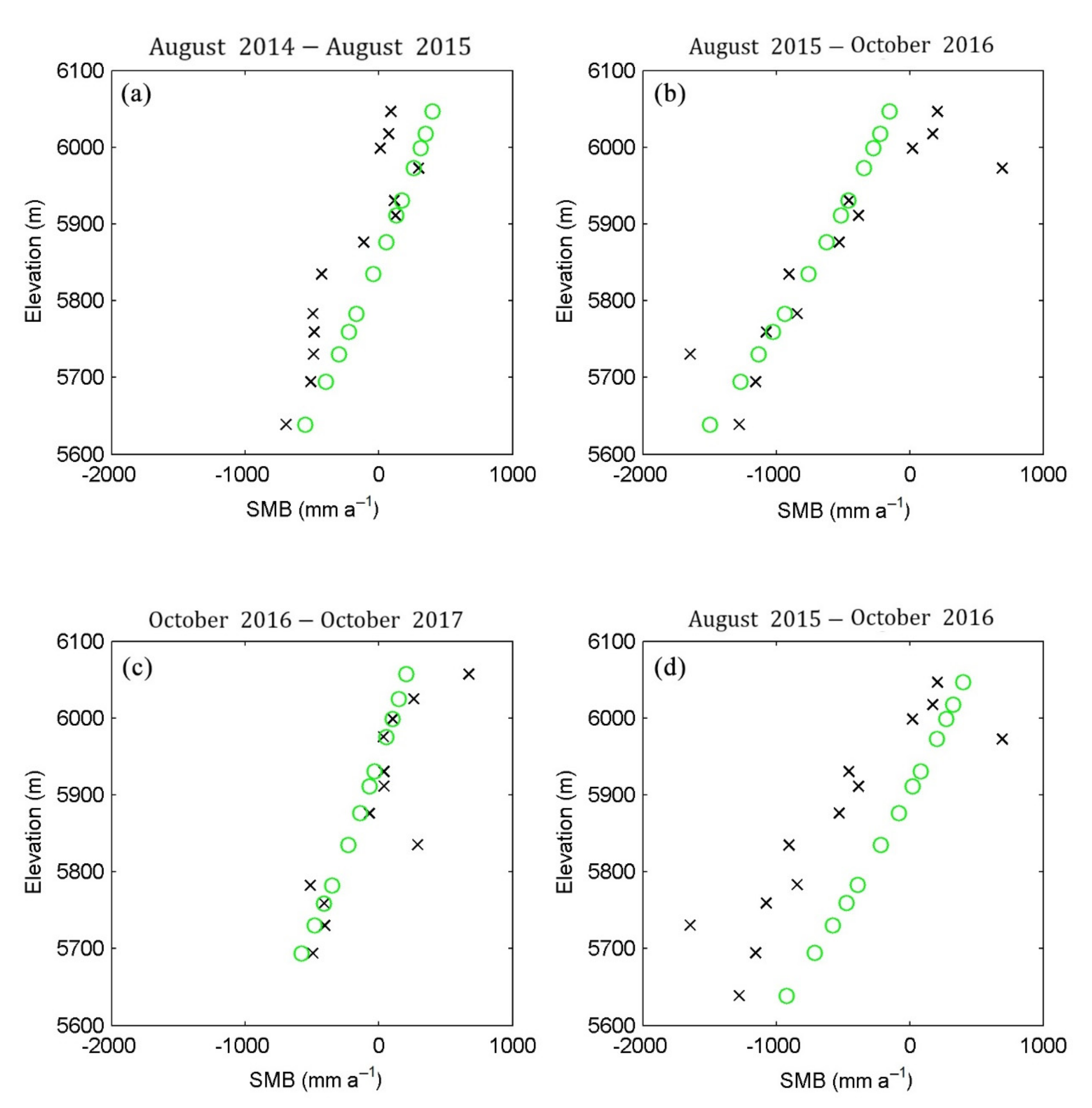
Figure 9.
Historical annual mean temperature (a) and summer mean temperature (b) at the elevation of AWS from Shiquanhe station from 1980 to 2017 (black), and the future annual mean temperature projected by RegCM4 under RCP2.6 (blue) and RCP8.5 (red) from 2006 to 2098 driven by 3 ESMs (HadGEM2ES, MPI−ESM−MR, NorESM1−M). Thick lines represent ensemble means.
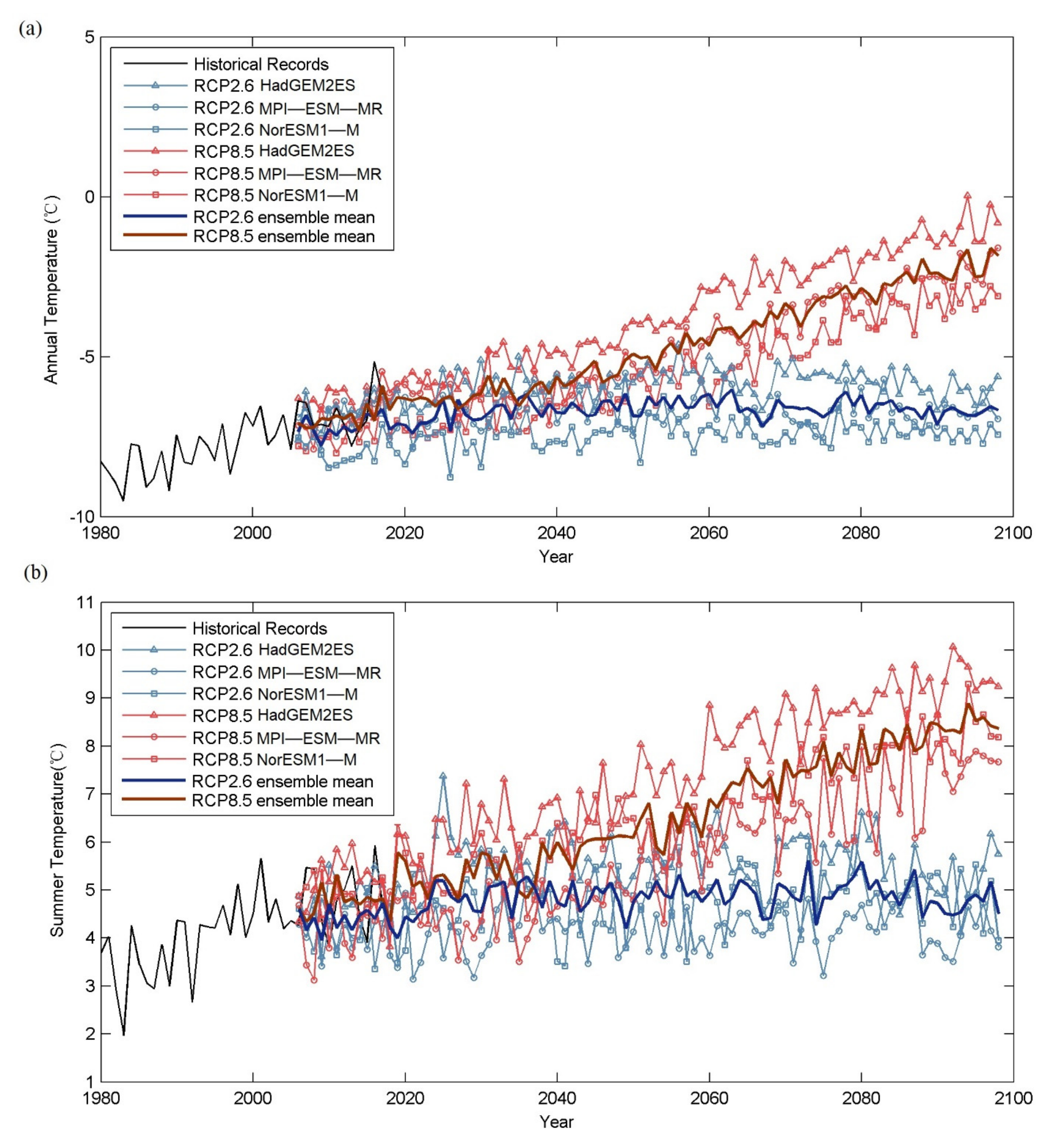
Figure 10.
The estimated surface (a), bed (b), and ice thickness (c) distributions for the year 2016.
Figure 10.
The estimated surface (a), bed (b), and ice thickness (c) distributions for the year 2016.
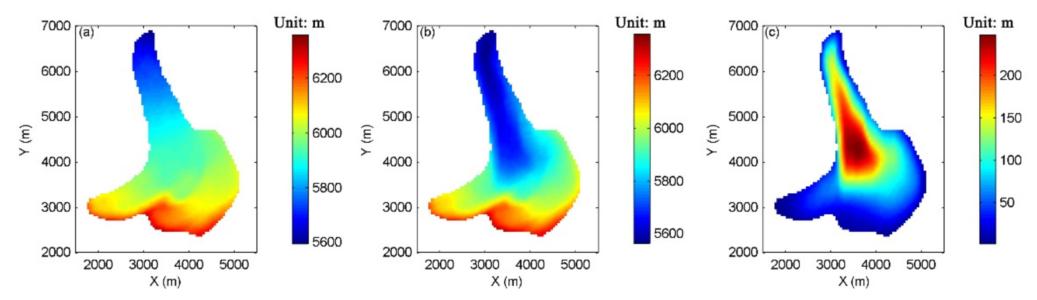
Figure 11.
(a) The observed surface velocities at stakes (stars), best-fit modeled with geothermal heat flux of 50 (triangles) and 60 (squares) mW m−2 (see legend hf50, hf60), and annual mean surface velocities provided by the NASA MEaSUREs ITS_LIVE project [21] satellite images (lines, see legend nasa) in the year 2015/2016 (blue) and 2016/2017 (red); (b) the averaged observed (red arrow) and modeled (blue arrow) surface velocities in the years 2015 and 2016 as vectors on the glacier surface.
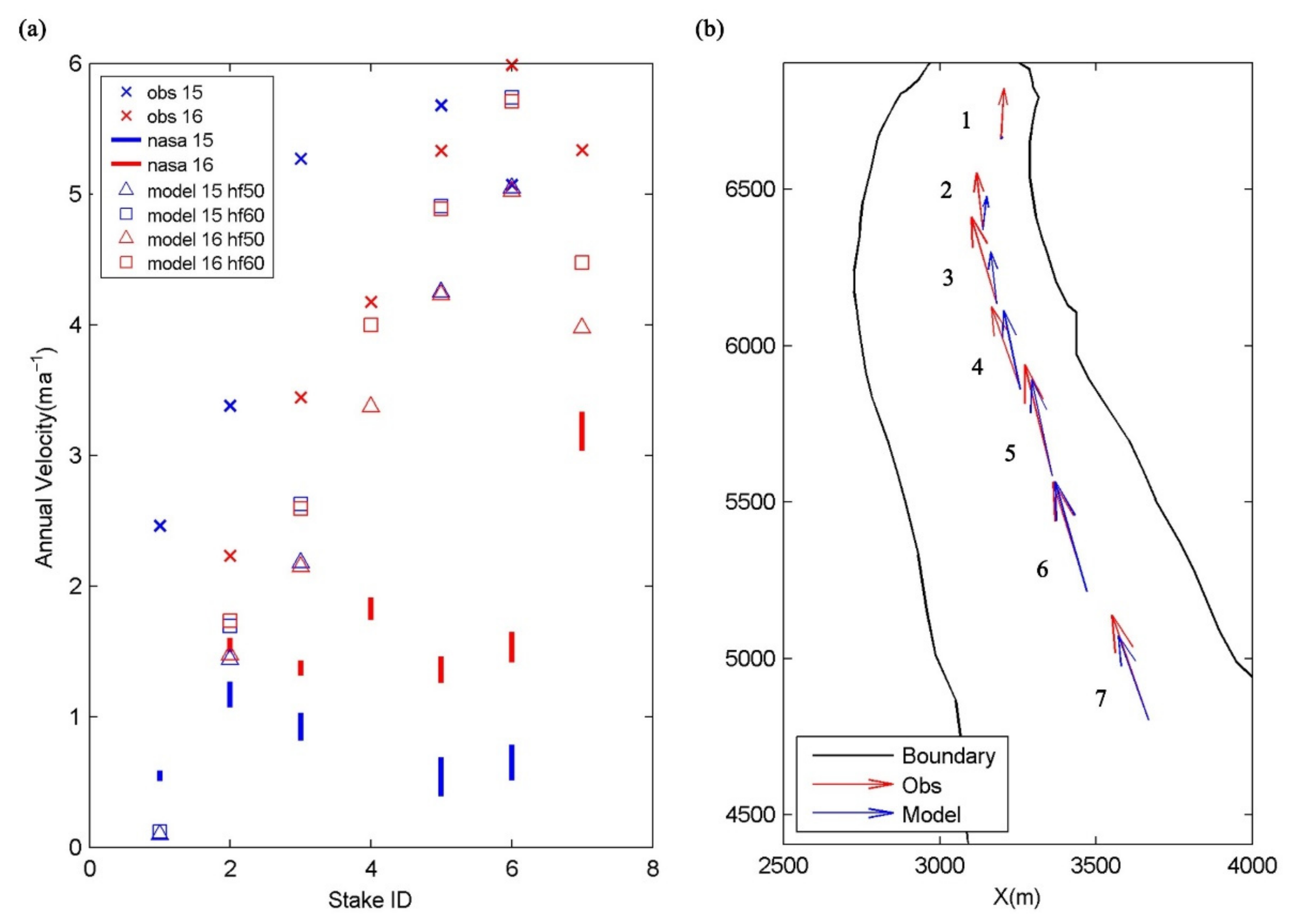
Figure 12.
Distribution of temperature relative to pressure melting point at the bedrock with geothermal heat flux of 50 (a) and 60 (b) mW m−2.
Figure 12.
Distribution of temperature relative to pressure melting point at the bedrock with geothermal heat flux of 50 (a) and 60 (b) mW m−2.

Figure 13.
Modeled surface velocities in the year 2016 with geothermal heat flux of 50 (a) and 60 (b) mW m−2.
Figure 13.
Modeled surface velocities in the year 2016 with geothermal heat flux of 50 (a) and 60 (b) mW m−2.
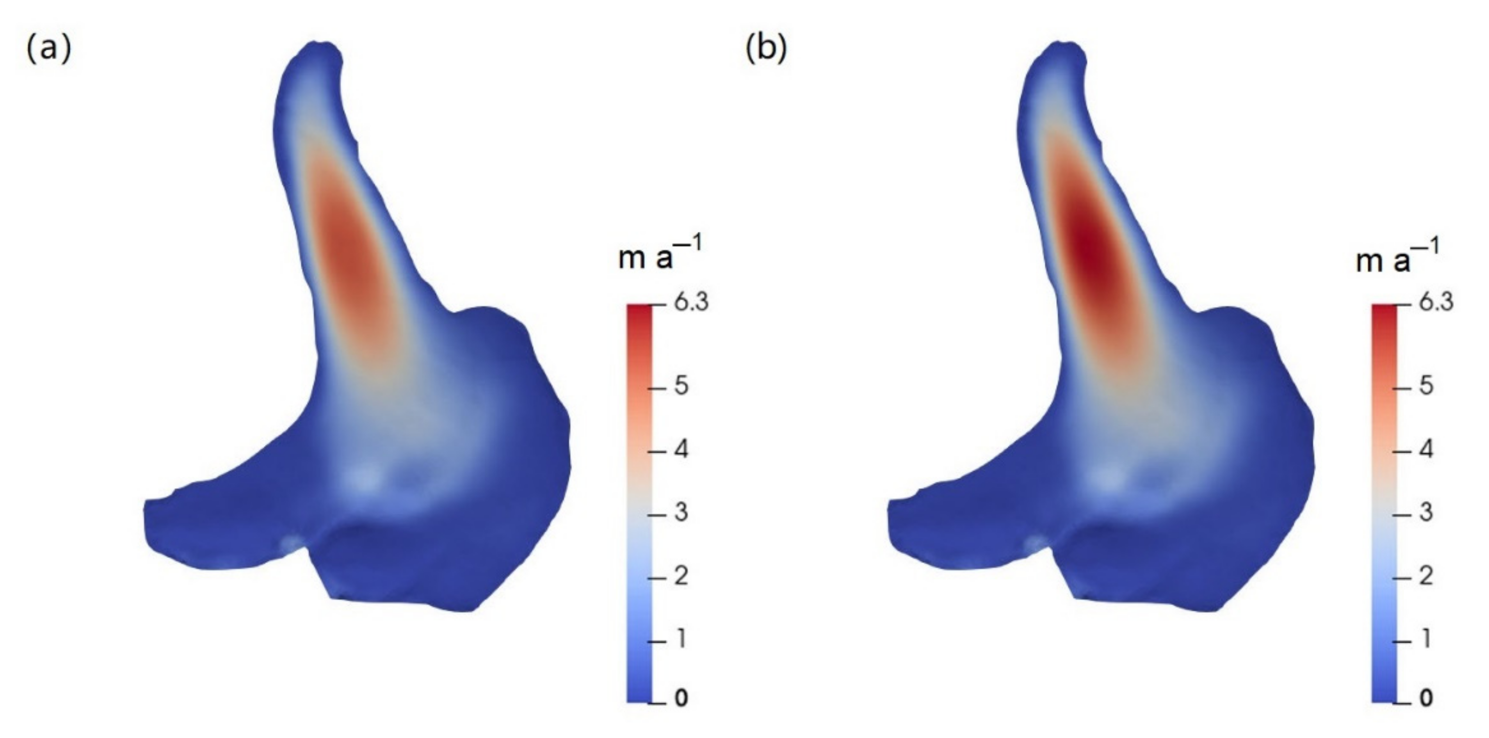
Figure 14.
Modeled ensemble mean volume changes from 2016 to 2098 using RegCM4 outputs driven by the 3 ESMs (HadGEM2−ES, MPI−ESM−MR, and NorESM1−M) for the period 2017−2098 under RCP2.6 (blue) and RCP8.5 (red), with ice dynamics (solid line) and without dynamics (dashed line). The across-model spread with/without ice dynamics are denoted by shading under RCP2.6 (blue/green) and RCP8.5 (red/pink).
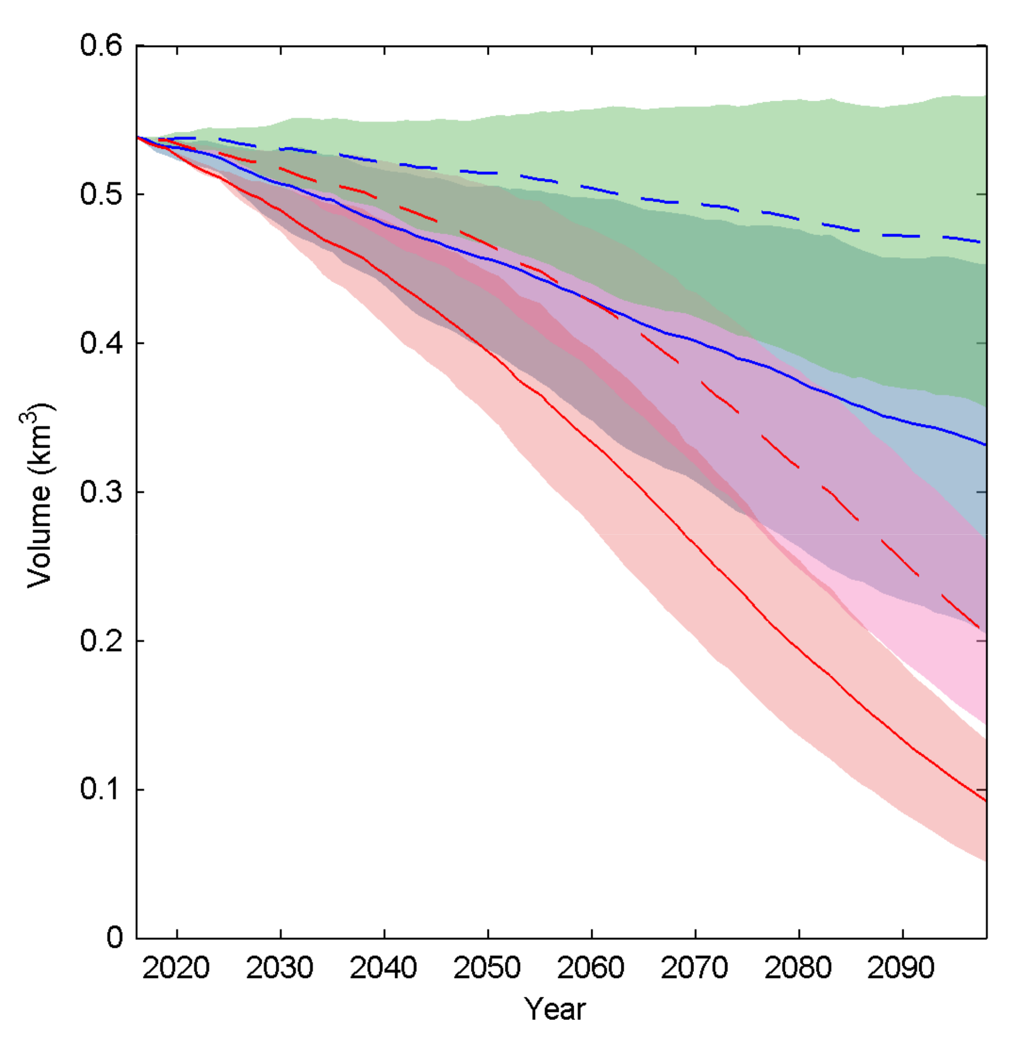
Figure 15.
Modeled terminus retreat from 2016 to 2098 under RCP2.6 (upper row, plot (a–c)) and RCP 8.5 scenarios (lower row, plot (d–f)) using projected results from RegCM4 driven by 3 ESMs, HadGEM2ES (plot (a,d)), MPI−ESM−MR (plot (b,e)), NorESM1−M (plot (c,f)).
Figure 15.
Modeled terminus retreat from 2016 to 2098 under RCP2.6 (upper row, plot (a–c)) and RCP 8.5 scenarios (lower row, plot (d–f)) using projected results from RegCM4 driven by 3 ESMs, HadGEM2ES (plot (a,d)), MPI−ESM−MR (plot (b,e)), NorESM1−M (plot (c,f)).

Table 1.
Modeled annual and summer mean temperature warming rate (°C·a−1) at the elevation of AWS projected by RegCM4 driven by 3 ESMs under RCP2.6 and RCP8.5 from 2018 to 2098.
Table 1.
Modeled annual and summer mean temperature warming rate (°C·a−1) at the elevation of AWS projected by RegCM4 driven by 3 ESMs under RCP2.6 and RCP8.5 from 2018 to 2098.
| HadGEM2ES | MPI−ESM−MR | NorESM1−M | Ensemble Mean | |
|---|---|---|---|---|
| RCP2.6 annual | 0.008 | 0.002 | 0.007 | 0.006 |
| RCP8.5 annual | 0.068 | 0.056 | 0.054 | 0.059 |
| RCP2.6 summer | 0.005 | 0.002 | 0.007 | 0.005 |
| RCP8.5 summer | 0.053 | 0.043 | 0.043 | 0.047 |
Publisher’s Note: MDPI stays neutral with regard to jurisdictional claims in published maps and institutional affiliations. |
© 2022 by the authors. Licensee MDPI, Basel, Switzerland. This article is an open access article distributed under the terms and conditions of the Creative Commons Attribution (CC BY) license (https://creativecommons.org/licenses/by/4.0/).
Share and Cite
MDPI and ACS Style
Zhao, W.; Zhao, L.; Tian, L.; Wolovick, M.; Moore, J.C. Simulating the Evolution of Da Anglong Glacier, Western Tibetan Plateau over the 21st Century. Water 2022, 14, 271. https://doi.org/10.3390/w14020271
AMA Style
Zhao W, Zhao L, Tian L, Wolovick M, Moore JC. Simulating the Evolution of Da Anglong Glacier, Western Tibetan Plateau over the 21st Century. Water. 2022; 14(2):271. https://doi.org/10.3390/w14020271
Chicago/Turabian StyleZhao, Wenqing, Liyun Zhao, Lide Tian, Michael Wolovick, and John C. Moore. 2022. "Simulating the Evolution of Da Anglong Glacier, Western Tibetan Plateau over the 21st Century" Water 14, no. 2: 271. https://doi.org/10.3390/w14020271
Note that from the first issue of 2016, this journal uses article numbers instead of page numbers. See further details here.