
Review of a Semi-Empirical Modelling Approach for Cohesive Sediment Transport in River Systems


Krishnappan Environmental Consultancy, Hamilton, ON L9C 2L3, Canada
Water 2022, 14(2), 256; https://doi.org/10.3390/w14020256
Submission received: 15 December 2021
/
Revised: 13 January 2022
/
Accepted: 14 January 2022
/
Published: 16 January 2022
(This article belongs to the Special Issue Modelling of River Flows, Sediment and Contaminants Transport)
Abstract
:In this paper, a review of a semi-empirical modelling approach for cohesive sediment transport in river systems is presented. The mathematical modelling of cohesive sediment transport is a challenge because of the number of governing parameters controlling the various transport processes involved in cohesive sediment, and hence a semi-empirical approach is a viable option. A semi-empirical model of cohesive sediment called the RIVFLOC model developed by Krishnappan is reviewed and the model parameters that need to be determined using a rotating circular flume are highlighted. The parameters that were determined using a rotating circular flume during the application of the RIVFLOC model to different river systems include the critical shear stress for erosion of the cohesive sediment, critical shear stress for deposition according to the definition of Partheniades, critical shear stress for deposition according to the definition of Krone, the cohesion parameter governing the flocculation of cohesive sediment and a set of empirical parameters that define the density of the floc in terms of the size of the flocs. An examination of the variability of these parameters shows the need for testing site-specific sediments using a rotating circular flume to achieve a reliable prediction of the RIVFLOC model. Application of the model to various river systems has highlighted the need for including the entrapment process in a cohesive sediment transport model.
1. Introduction
Cohesive sediments play an important role in the transportation of contaminants and nutrients in a river system. Cohesive sediments are characterized as a mixture of predominantly clay- and silt-sized fractions of clay-type minerals but may also contain a range of organic compounds [1]. Contaminants and nutrients interact with these cohesive sediment mixtures and become part of the assemblage of the mineral and organic particles due to physical, chemical and biological controls [2]. Therefore, the contaminants and nutrients are transported in the river systems predominantly in association with cohesive sediments. A better understanding of the transport processes of cohesive sediment is of paramount importance for understanding the water quality and the quality of the river ecosystem.
Transport processes of cohesive sediment were studied extensively in the literature for over sixty years. The pioneering work in this area was carried out by Partheniades [3,4,5], Partheniades and Kennedy [6] and Partheniades et al. [7]. Partheniades used a rotating circular flume to study the physical behavior of cohesive sediments in the laboratory and concluded that the cohesive sediment behavior is very different from that of the cohesionless coarse-grained sediments, which had been studied extensively in this area of research (see, e.g., [8,9,10]). Among the differences in the transport behaviors between cohesive and cohesionless sediments, the one that sets them apart is the flocculation process. Because of the fineness of the cohesive sediments, the surface forces of attraction and repulsion become the same order of magnitude as the body (gravity) forces. As a consequence, the cohesive sediments undergo the process of flocculation in which the cohesive sediment particles interact and become agglomeration of particles called flocs [3,7,11,12,13,14,15]. Cohesionless sediments, on the other hand, behave as individual particles in a flow field.
Analysis of cohesive sediment transport in a flow field is much more difficult in comparison to the analysis of cohesionless sediment. Since the cohesionless sediment behaves as individual particles and the density of the particles is also constant (~2.65), the settling velocity of the cohesionless sediment is well defined for a sediment of a certain size (Stokes Law). The same cannot be said for the cohesive sediment. In the case of cohesive sediment, because of the flocculation process, the size of the transporting unit in a flow field is a variable and depends, among other things, on the intensity of the flow field, which can break up the flocs into smaller units. Moreover, the density of the transported unit is also variable as a result of the incorporation of suspending fluid into the floc structure. Therefore, the specification of settling velocity for cohesive sediment is much more difficult than for the cohesionless sediment.
In addition, the erosion and deposition characteristics of cohesive and cohesionless sediments are also different. From his laboratory studies, Partheniades [3] concluded that for cohesive sediments, the critical shear stress for erosion is different from the critical shear stress for deposition, and at a particular bed shear stress, cohesive sediments undergo either erosion or deposition but not both simultaneously. Cohesionless sediments, on the other hand, have only one critical condition that is valid for both erosion and deposition and undergo simultaneous erosion and deposition processes under all bed shear stress conditions.
Earlier research had treated the cohesive sediment as part of the “wash load”, which was defined as the sediment load consisting of grain sizes that are considerably finer than those present in the stream bed [8]. It was further assumed that the wash load is “supply limited” and its transport rate is independent of flow characteristics. However, recent research has shown that the cohesive sediments do interact with stream beds and the transport characteristics of cohesive sediments, including the flocculation mechanism, do depend on flow characteristics [3,4,7,11,12,13,14,15,16,17].
When modelling the transport of cohesive sediments in rivers, the aforementioned differences between the cohesive and cohesionless sediments have to be taken into account rather than simply extending the cohesionless sediment transport models to cohesive sediment as has often been done in the literature. In cohesionless transport models, a mass balance equation is usually solved with the critical shear stress for erosion, as given by the Shield’s diagram and employing any one of the numerous sediment transport formulae that have been derived experimentally for these types of sediments. For cohesive sediments on the other hand, the critical shear stress conditions for erosion and deposition that are universally accepted are not available and the sediment transport rate functions are also not readily available. The flocculation process also needs to be taken into account. Under these circumstances, the modelling of cohesive sediment transport in river systems requires a fresh approach that will address the unique nature of cohesive sediment transport processes such as flocculation and the distinctive erosion and deposition processes that the sediment experiences over a certain range of bed shear stresses prevailing in a river system. An examination of the flocculation process and the erosion deposition processes is undertaken here to highlight the complexities of a cohesive sediment transport model.
1.1. Flocculation Process
Early studies on the flocculation of cohesive sediments were carried out in estuarial systems where the mixing of freshwater from the river with the salt water in the ocean caused the river sediments to flocculate [3,18]. In these studies, the flocculation process was treated as a two-step process; in step one, called the “collision process”, the particles are made to collide against each other by processes such as Brownian motion, turbulence, velocity gradients, inertia and differential settling, and in step two, called the “cohesion process” the collided particles are bonded together to form an agglomeration of particles called flocs. In estuarine systems, the bonding or the cohesion was provided by the relative strengths of attractive versus repulsive forces between the particles. The attractive forces are due to van der Waal’s forces, which vary inversely as the seventh power of the distance between the particles. The repulsive forces are due to the like charges of the ion clouds surrounding the clay particles [18].
In recent studies on flocculation, cohesive sediments were observed to form flocs even in freshwater systems [19,20,21]. The cohesion mechanism involved in the freshwater flocculation is different from the one found in estuarine systems. In freshwater flocculation, bacteria and other microorganisms were found to play a role in the floc formation [2,21,22]. The microorganisms secrete polymers [23], which provide the bonding among particles. The mechanism of flocculation by polymers can be explained on the basis of the classical interparticle bridging model described in Ruehrwein and Ward [24] and La Mer and Healy [25]. Busch and Stumm [26] reported that the amount of polymers required for optimal flocculation is extremely small, of the order of a mg/L.
1.2. Distinct Nature of Erosion and Deposition Processes of Cohesive Sediment
A better understanding of the erosion and deposition processes governing the transport of sediment in a river system is important for modelling the sediment fluxes at the sediment–water interface. The settling and the dispersive fluxes at the sediment–water interface is balanced by the net amount of sediment entering the flow domain from the bed. For cohesionless sediments at a given bed shear stress greater than the critical shear stress for erosion, the deposition and erosion of the sediment occur simultaneously, and for a steady state condition, the deposition flux is equal to the erosion flux. For the cohesive sediment, on the other hand, since the deposition and the erosion processes are mutually exclusive, there is only one flux at a time, either a deposition flux or an erosion flux. The existence of two different critical conditions for the cohesive sediment can be explained as follows: when a cohesive sediment floc deposits onto a bed consisting of cohesive sediment flocs, the deposited floc sticks to the flocs that are part of the bed due to cohesion and requires a slightly higher bed shear stress to dislodge the deposited floc from the bed. Therefore, for cohesive sediments, two distinctive critical shear stresses can be identified, one for deposition and the other for erosion: the critical shear stress for erosion is always higher than the critical shear stress for deposition.
The erosion characteristics of cohesive sediment have been studied extensively in the literature [3,6,7,11,12,13,14,27,28,29,30,31]. These studies have shown that the erosion characteristics of cohesive sediment deposits depend on a number of parameters, including the manner in which the sediment deposit is created, the time of consolidation, the rate of application of the bed shear stress and the stabilizing effects of the microorganisms. A comprehensive list of all the governing parameters that control the erosion process of cohesive sediment deposits can be found in Hayter [32].
Because of the numerous controlling parameters involved in both the flocculation process and the erosion and deposition processes of cohesive sediment, it is practically impossible to derive analytical expressions representing the flocculation and the erosion and deposition processes of cohesive sediment transport. Therefore, the approach of a semi-empirical formulation of a mathematical model to represent the transport of cohesive sediment becomes attractive for finding practical solutions to problems pertaining to the transport of cohesive sediment and the associated contaminants. Krishnappan [33,34] developed a cohesive sediment transport model for rivers (RIVFLOC) and employed a semi-empirical approach to determine the parameters of the model by carrying out experiments in a rotating circular flume for site-specific sediment and the river water. Using these parameters, the model can then be applied to the actual rivers to predict the transport of cohesive sediment and the associated contaminants. This modelling approach had been used successfully to a number of river systems [34,35,36,37,38,39]. In this review paper, the RIVFLOC model of Krishnappan [33,34] is described highlighting the model parameters and their determination using a rotating circular flume. The variability of the model parameters of different river systems is also examined. The objective of this review is to provide guidance for modelling cohesive sediment transport and the associated contaminants in a river system.
2. Materials and Methods
2.1. Description of the RIVFLOC Model
The RIVFLOC model predicts the transport of fine-grained, cohesive sediments in rivers. It has two components: a transport and dispersion component and a flocculation component. The transport and dispersion component is based on the advection-diffusion equation expressed in a curvilinear co-ordinate system to treat the transport and mixing of fine sediment entering a river as steady source. The flocculation component adapts a coagulation equation that includes four different collision mechanisms and treats the process of agglomeration of the fine sediment as it is transported in a river flow. Details of the model are described in Krishnappan [33]. Here, some salient features of the model are described for the sake of completeness.
2.1.1. Transport and Dispersion Component
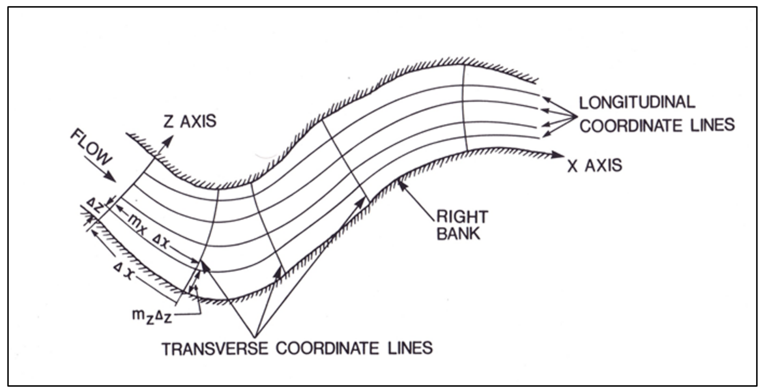
A depth-averaged advection-dispersion equation expressed in the curvilinear co-ordinate system (Figure 1) introduced by Yotsukura and Sayre [40] is used to analyze the transport and dispersion process of fine sediment in the RIVFLOC model. The form of the equation solved is shown below:
where
Ck = depth-averaged volumetric concentration of the kth size fraction.
x = distance along the longitudinal co-ordinate axis (Figure 1).
U = depth-averaged velocity component in the x direction.
h = depth of flow.
Q = flow rate.
Ez = transverse dispersion coefficient.
Mx, = metric coefficients of the curvilinear co-ordinate system.
η = normalized cumulative discharge given by:
.
z = transverse co-ordinate.
λ1 = rate coefficient for reaction.
λ2 = rate of sediment source or sink.
Boundary conditions needed to solve the mass balance equation are as follows:
- For the upstream boundary, a known transverse distribution of fine sediment entering the river has to be specified together with the size distribution of the sediment. This can be obtained either by direct measurement or from some other calculations.
- At the side banks, the sediment fluxes crossing these banks are zero, and hence the concentration gradients across those boundaries are taken as zero.
- At the bed, the sediment fluxes across the sediment–water interface need to be specified. Transfer of sediment between the bed and water column can occur because of the following three processes, namely, erosion, deposition and entrapment (ingress of fines in coarse bed sediment). The first two processes were studied extensively in the literature. For example, the erosion rate of fine sediment has been studied by Partheniades [3], Mehta and Partheniades [41], Parchure [30], Lick [13], and Krishnappan et al. [42]. Deposition characteristics of fine sediment were studied by Krone [11], Mehta and Partheniades [12], Lick [13], among others.
In the RIVFLOC model, Krone’s approach was used to specify the net deposition of fine sediment to the river bed. According to this approach, the net deposition flux (qd) was calculated as:
where P represents the probability that a floc, settling to the bed, stays at the bed (a stickiness parameter). is the settling velocity of sediment and is the near-bed concentration of the kth size fraction of the sediment. Krone [11] proposed a relationship for P as:
where is the bed shear stress and is the critical shear stress for deposition, which was defined by Krone as the bed shear stress above which none of the initially suspended sediment would deposit. The bed shear stress τ (together with the flow field) has to be determined using a hydrodynamic model for the river flow. The critical shear stress for deposition has to be determined experimentally for site-specific sediments using specialized experimental facilities such as a rotating circular flume.
For bed shear stresses greater than , deposition flux will be zero, but erosion flux can exist. In the RIVFLOC model, the erosion flux was modelled using an erosion rate proposed in Krishnappan et al. [42]. Accordingly,
where E is given by:
where are constants to be determined from laboratory experiments using a rotating flume for site-specific sediment and t is the elapsed time from the stress change during a particular shear stress step.
Unlike erosion and deposition, the entrapment process is not studied extensively in the literature. In an empirical study carried out by Krishnappan and Engel [43], it was shown that the entrapment flux can be related to the settling flux through a proportionality coefficient, termed entrapment coefficient. According to this study, the entrapment flux () can be is expressed as:
where is the entrapment coefficient. This entrapment coefficient can be a function of porosity of the gravel substrate, thickness of the gravel bed layer and the permeability of the gravel substrate, but a quantitative relationship involving these parameters is not available at the present time.
2.1.2. Flocculation Stage
The flocculation stage was based on a coagulation equation (Fuchs [46]) shown below:
where and are number concentrations of particle size classes i and j, respectively. is the collision frequency function, which is a measure of the probability that a particle of size i collides with a particle of size j in unit time, and β is the cohesion factor, which defines the probability that a pair of collided particles will coalesce and form a new floc. The cohesion factor accounts for the different cohesion mechanisms such as the electrochemical cohesion that occurs in estuaries where the freshwater meets the salt water and in the freshwater systems, where the cohesion occurs due to polymers secreted by micro-organisms, etc. In this study, β is treated as an empirical parameter and was determined through the calibration of the model using experimental data.
Equation (7) was simplified by considering the particle sizes in discrete size classes as shown in Figure 2. In this figure, the continuous particle size space is considered in discrete size ranges (1 to M). Each range is considered as a bin containing particles of a certain size range. For example, r1 is the geometric mean radius of particles in bin 1. The particle ranges were selected in such a way that the mean volume (vi) of particles in bin i is twice that of the preceding bin. The volume ranges of the various size ranges are shown in Figure 2.
Under this scheme, when particles of bin i flocculate with particles in bin j (j < i), the newly formed particles will fit into bins i and i + 1. The proportion of particles belonging to these bins can be calculated by considering the mass balance of particles before and after flocculation (allocation function). With this simplification, the coagulation equation is expressed in discrete form as follows:
where is the allocation function given by:
where is the density of the flocs and V is the volume of the flocs. The density of the flocs is dependent on their size, and an empirical relationship between the two was formulated by Lau and Krishnappan [47]. This relationship was adopted for the present study. The form of the relationship is as follows:
where , and are densities of flocs, water and parent material forming the flocs, respectively. D is the diameter of the floc and b and c are empirical coefficients to be determined from rotating flume experiments in the laboratory. The settling velocity of flocs, needed for the settling stage of the particle motion, was calculated using Equation (10) and the Stoke’s Law. The resulting expression is as follows:
where g represents the acceleration due to gravity and stands for the kinematic viscosity of water.
The collision frequency function assumes different functional forms depending on the collision mechanisms that bring the particles to close proximity. The mechanisms considered in this study are (1) Brownian motion (), (2) turbulent fluid shear (), (3) inertia of particles in turbulent flow () and (4) differential settling of flocs (). An effective collision frequency function, , was calculated in terms of the individual collision functions as follows:
The individual collision frequency functions were formulated by Valioulis and List [48], and the form of the functions are as follows:
For Brownian motion:
For fluid shear:
For inertia:
For differential settling:
The symbols appearing in the above collision frequency functions have the following meanings: K is the Boltzmann constant, T is the absolute temperature in degree kelvin, is the viscosity of fluid, is the kinematic viscosity, is the turbulent energy dissipation per unit mass, and and are densities of sediment and fluid, respectively.
The break-up of flocs due to turbulent fluctuations of the flow was modelled using a method proposed by Tambo and Watanabe [49]. According to this method, a “collision-agglomeration” function was introduced as a multiplier to the collision frequency function, . This resulted in an optimum floc size distribution for a given level of turbulence. The function proposed by Tambo and Watanabe is given below:
where R is the number of primary particles in a floc and Rm is the number of particles in the biggest floc for the given level of turbulence. The parameters and n take on values of 1/3 and 6, respectively.
The input data requirement for the RIVFLOC model and the possible sources of such data are summarized in Table 1 below:
2.2. A Computational Methodology for the Lateral Variation of the Longitudinal Velocity U
The development of the curvilinear coordinate system shown in Figure 1 requires knowledge of the depth-averaged longitudinal velocity component () distribution in the lateral direction and the depth variation across the river. The depth variation across the river can be obtained from the cross-sectional surveys. The depth-averaged velocity distributions are computed within the RIVFLOC model using a methodology proposed by Djordjevic [50] and Guan et al. [51]. According to this method, the depth-averaged momentum equation in the longitudinal direction is simplified as follows:
In the equation above, V is the depth-averaged velocity components in the transverse directions, zw is the water surface elevation above a datum, g and are the gravitational acceleration and water density, respectively, is the depth-averaged turbulent shear stress and is the bed shear stress. The depth-averaged turbulent shear stress is calculated using the eddy viscosity concept as:
where is the depth-averaged eddy viscosity coefficient. Assuming similarity with mass transport, is expressed as:
where is an empirical constant and is the shear velocity. The bed shear stress is expressed as:
where is the transverse angle of inclination of the bed to the horizontal, is the friction factor, which can be expressed in terms of the Manning’s n as:
Substituting Equations (19)–(21) into Equation (18), we get:
Assuming that the first term on the right-hand side of Equation (23) is small in comparison to the second term, and using Guan et al. [51] approximation for the product UV in the second term as:
Equation (23) can be expressed as follows:
The above equation is a second order ordinary differential equation with variable coefficients and can be solved numerically for the longitudinal velocity component U once the water surface slope appearing on the right-hand side of the equation is specified. For the RIVFLOC model, the water surface slope in the river reach was supplied by a one- dimensional mobile boundary flow model MOBED developed by Krishnappan [52,53,54]. The MOBED model solves the full St. Venant’s equations and a sediment mass balance equation to treat the coarse-grained sediment constituting the riverbed and calculates the bed level changes in addition to water level changes as a function of time and distance along the river reach. The model also supplies the bed shear stresses needed for the RIVFLOC model to model the cohesive sediment transport.
2.3. Determination of Model Parameters Using a Rotating Circular Flume
The model parameters that needed to be determined from laboratory experiments are: critical shear stresses for erosion and deposition, erosion rate, cohesion parameter, and the empirical coefficients defining the floc size and floc density relationship (see Table 1). For performing laboratory experiments with cohesive sediments, the rotating circular flumes are preferable than the straight flumes, as the pumping and other flow regulation devices that are associated with the straight flume are likely to disrupt the flocs and cause floc breakage. To avoid this from happening, rotating circular flumes are invariably used for cohesive sediment transport experiments in which the flocculation mechanism is often the main focus of the study.
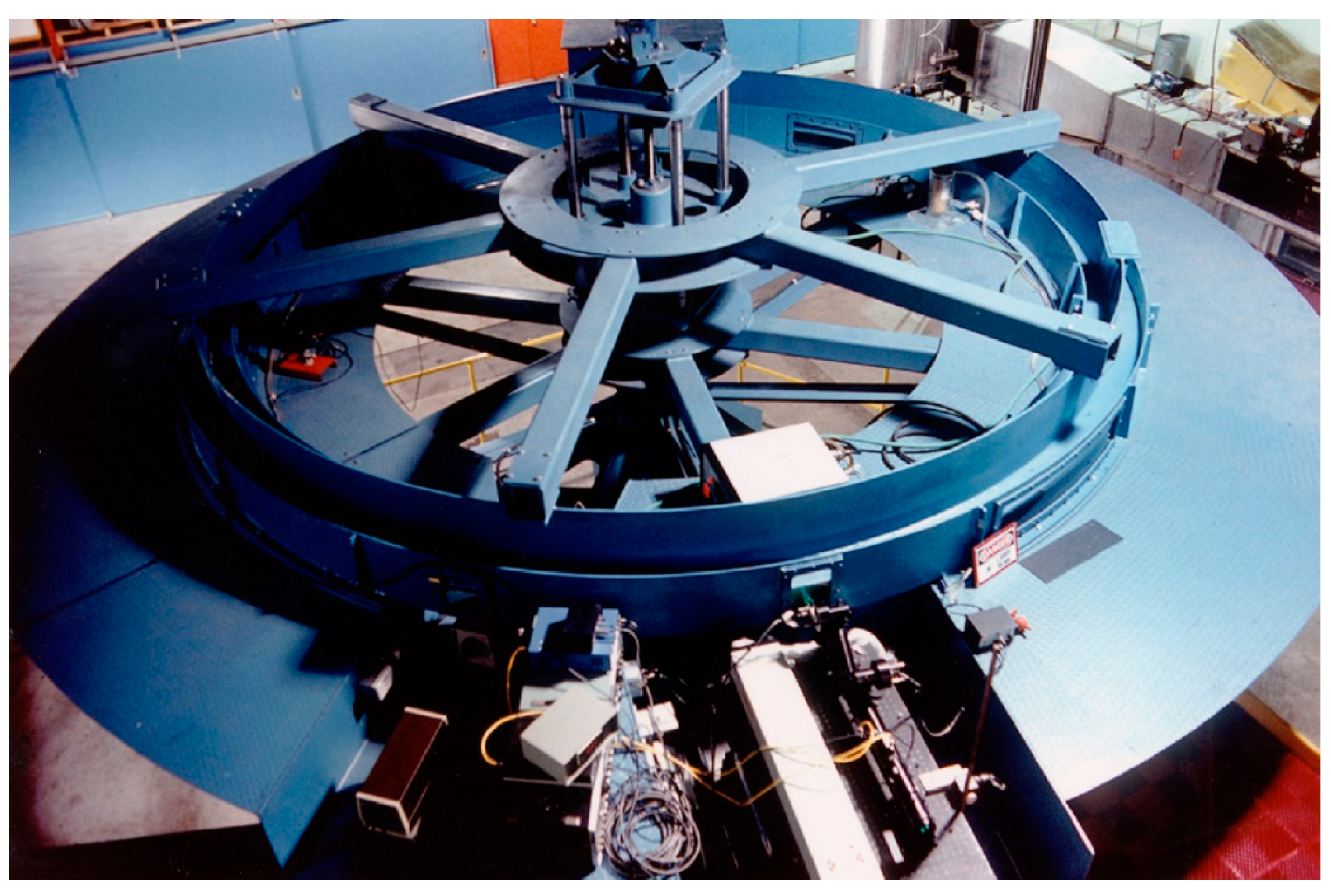
As part of a cohesive sediment transport research programme at the National Water Research Institute (NWRI) in Burlington, Ontario, Canada, a 5.0 m diameter circular flume was installed. Complete details of the flume can be found in Krishnappan [55]. Here, some of the salient features of the flume are highlighted. The flume is 5.0 m in diameter, 30 cm wide and 30 cm deep. It rests on a rotating platform, which is 7.0 m in diameter. A counter rotating top cover fits inside the flume with close tolerance and makes contact with the water surface. The simultaneous rotation of the flume and the top cover in opposite directions produces a flow field that is nearly two dimensional. A photograph showing the top view of the flume is shown in Figure 3.
The flow fields generated in this flume were studied extensively [56,57,58]. These studies have shown that the flows generated in the flume are nearly two dimensional and the bed shear stress distributions across the flume are fairly uniform, as shown in Figure 4.
In Figure 4, the bed shear stresses are plotted as a function of distance across the flume with rotational speed as the parameter. The points are measured values and the lines are calculated distributions using a 3D hydrodynamic flow model (PHOENICS) developed by Roston and Spalding [59]. It can be seen from this figure that the PHOENICS model predictions agree well with the measured values.
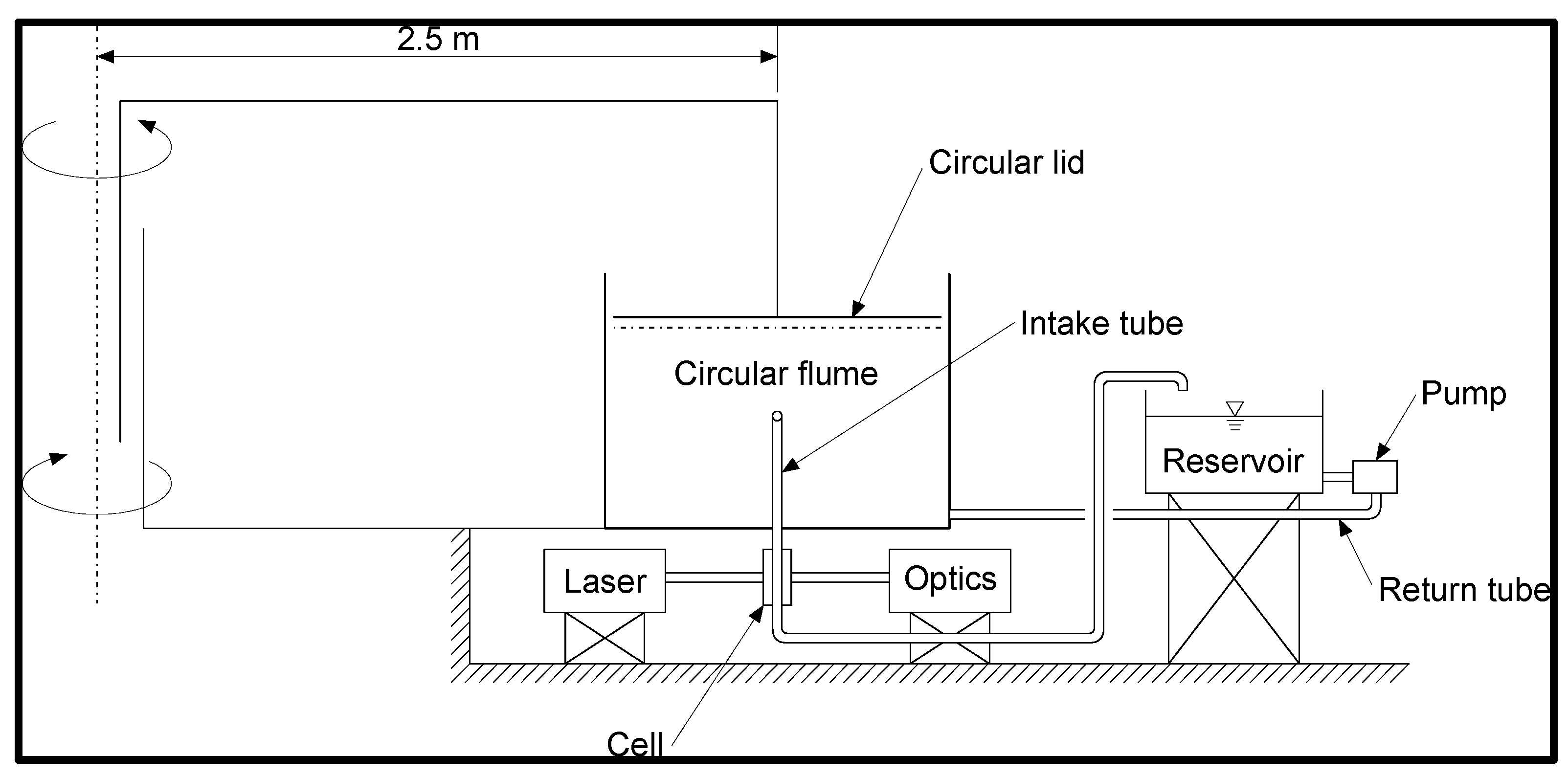
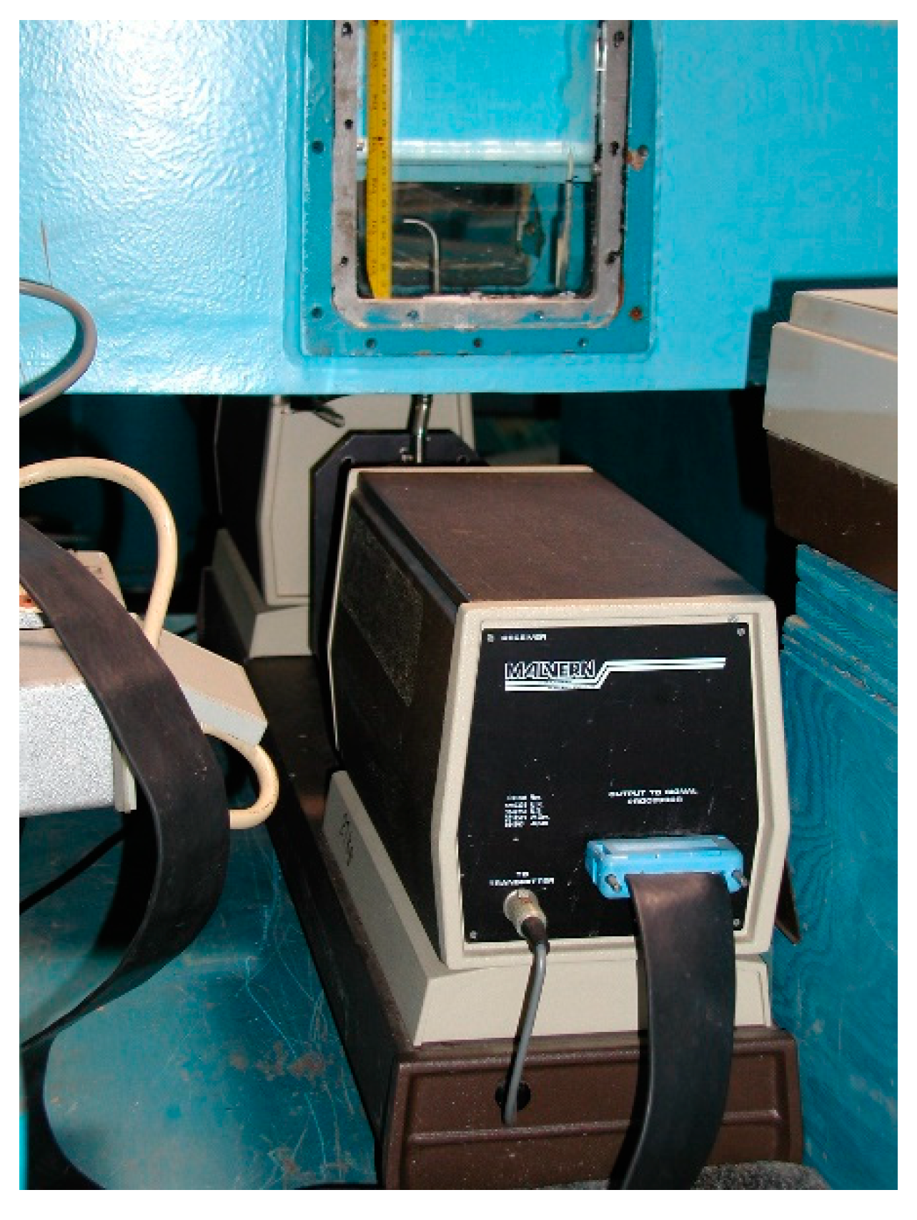
The flume is fitted with a Malvern Particle Size Analyser [60] for measuring the size distribution of suspended sediment flocs. The instrument was placed directly underneath the flume, and the short tube connects the sampling point to the sample cell of the instrument. The sample is drawn through the sample cell continuously by gravity, and the sample after passing through the sample cell flows into a reservoir from where it was pumped back into the flume. The arrangement of the instrument is shown in Figure 5 and a photograph of the set-up is shown in Figure 6.
2.4. Collection of Sediment Samples for Testing in the Rotating Circular Flume
The samples of sediment–water mixtures were collected from the study areas in the field and were brought to the laboratory for testing in the rotating circular flume. The sampling device that was used for this purpose is described here. It is an inverted cone sampler specially designed for this purpose. The sampler consists of a conical chamber fitted with a propeller and a submerged pump. A photograph of the sampler is shown in Figure 7.
To collect the sediment–water mixture using the sampler, the sampler was deployed in a depositional area in a river and the propeller and the pump were turned on remotely from a boat or from the shore. The propeller creates a sufficiently strong currents to dislodge the deposited fine sediment from the bed into suspension and the sediment–water mixture is pumped from the sampler to a sample container by operating the submerged pump. The sampler is also fitted with a weight to stabilize the sampler on the streambed against the flow and an under-water video camera to observe the operation of the sampler. Normally about five hundred to one thousand litres of sediment–water mixtures would be collected and transported to the laboratory in refrigerated trucks to preserve the chemical and biological characteristics of the sample.
2.5. Testing of Cohesive Sediments Transport Characteristics in the Rotating Circular Flume
Both depositional and erosional characteristics of cohesive sediment samples were tested in the rotating circular flume. For depositional experiments, sediment–water mixture was placed in the flume and the sediment concentration was adjusted by adding additional cohesive sediment to produce a fully mixed concentration of known value. Full mixing of the sediment was achieved by operating the flume at high speeds (2.5 rpm for the lid and 2 rpm for the flume, which corresponds to a bed shear stress of 0.6 Pa) that were found to be sufficient to maintain all of the sediment in suspension. The high-speed operation of the flume was maintained for a period of about 20 min and then the speeds were lowered to their respective test speeds to yield a particular bed shear stress in the flume. The flume was operated at this level for about 5 h. During this time, suspended sediment concentration and the size distribution of the suspended sediments were monitored at regular intervals of time. Experiments were then repeated for different bed shear stress conditions maintaining the initial concentration to be the same for all these tests. The influence of the initial concentration was also tested by conducting set-up experiments in which the initial concentration was varied while the bed shear stress was kept constant.
Erosion experiments were carried out by allowing all the suspended sediment to settle to the bed and allowing the deposited sediment to consolidate for different time durations. To begin an erosion test, the flume and the lid were started from rest and their speeds were increased in steps and each step was maintained for a period of 40 to 90 min. During each step, sediment samples were collected and the concentration of the eroded sediment in the water column were determined as a function of time. When the concentration of the sediment is sufficiently high, size distribution of the eroded sediment was also measured.
3. Results
The semi-empirical model of cohesive sediment transport (RIVFLOC model) was applied to different river systems to assess the cohesive sediment and associated contaminants in these systems. The listings of some of these studies are given in Table 2 along with the model parameters that were determined using the rotating flume for site-specific sediments.
The methodologies used to determine the model parameters using the results from the depositional and erosional experiments for site-specific sediments carried out in the rotating circular flume are reviewed here in the following subsection. The experimental results for the Hay River sediment [34] are used as an example.
3.1. Determination of Critical Shear Stress for Deposition
The results from the deposition experiments carried out in the rotating circular flume for the Hay River sediment are summarized in Figure 8.
Figure 8 shows the concentration variation of the suspended sediment as a function of time for different bed shear stresses as the sediment undergoes deposition. For a particular shear stress, concentration of sediment in suspension decreases initially as a function of time and reaches a steady state concentration, which is a function of the shear stress. When the shear stress is high, the steady state concentration is high, and a majority of initially suspended sediment stays in suspension (about 90% for the shear stress of 0.323 Pa). For lower shear stress tests, the concentration of sediment that stays in suspension diminishes, and for the lowest shear stress tested (0.088 Pa), the concentration of sediment in suspension is only about 10% of the initial sediment concentration. If the bed shear stresses were slightly lower than the lowest shear stress tested, all of the initially suspended sediment would have settled to the bed. Such a bed shear stress is termed the critical shear stress for deposition (: Partheniades’ definition of critical shear stress for deposition). For Hay River sediment tested here, it can be determined by extrapolation that the critical shear stress for deposition was 0.08 Pa.
3.2. Determination of Critical Shear Stress for Erosion and the Erosion Rate
Results from the erosion experiments carried out for the Hay River sediments are shown in Figure 9.
The erosion experiments for the Hay River sediment were carried out for two different consolidation periods (one-day consolidation and two-day consolidation). As can be seen from Figure 9, for one-day consolidation, the onset of erosion occurs at a bed shear stress of 0.12 Pa, whereas for the two-day consolidation it is at 0.16 Pa, which shows that the consolidation process plays an important role in determining the erosion characteristics of Hay River sediments. For this sediment, the critical shear stress for erosion was taken as 0.14 Pa, which is an average of the two consolidation period experiments. The erosion rate function (i.e., Equation (5)) can be established for this sediment using the approach of Krishnappan et al. [42].
3.3. Influence of Initial Concentration on the Deposition Process
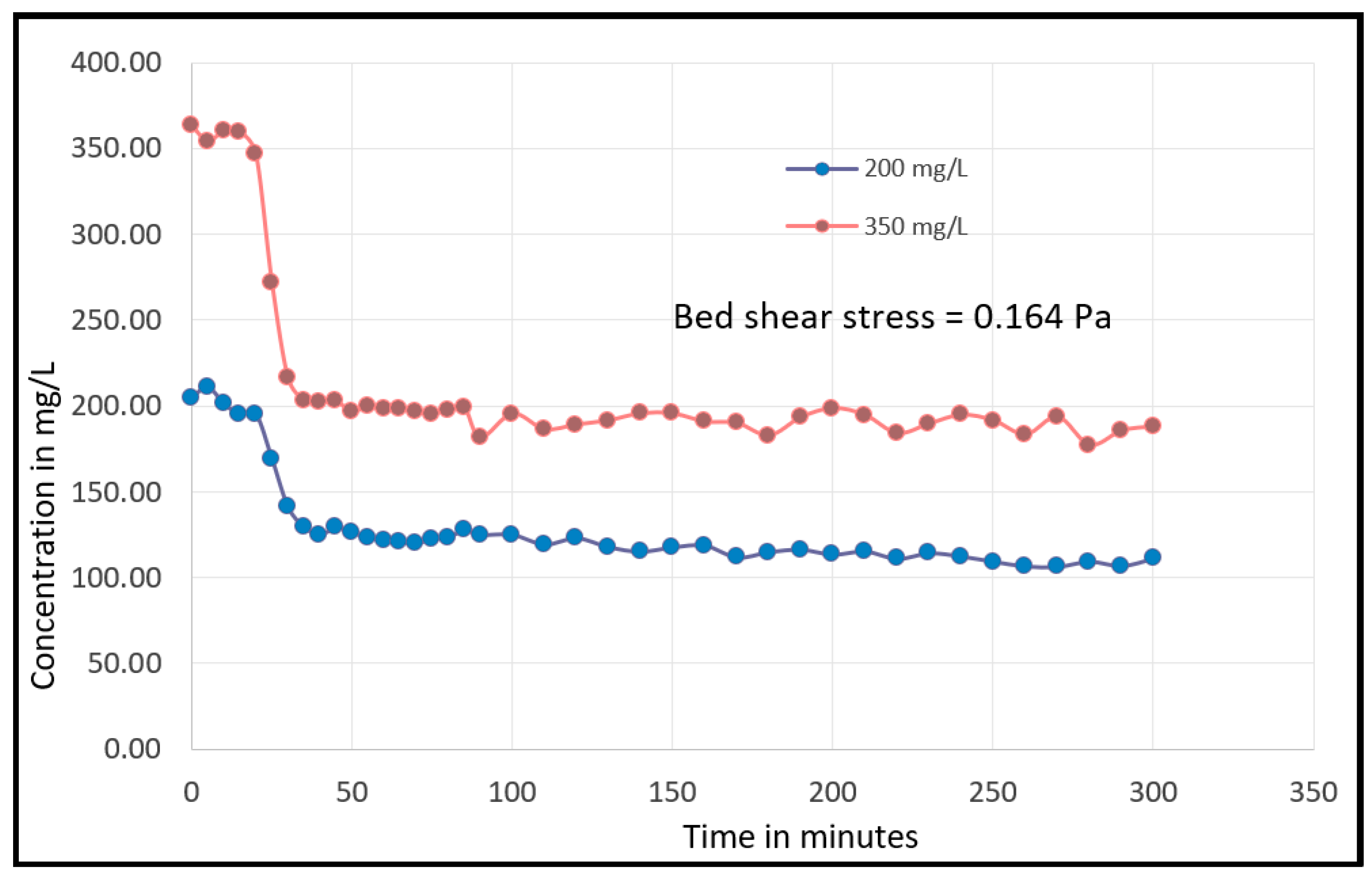
Experiments were carried in the rotating circular flume to test the influence of the initial concentration on the deposition process by varying the initial concentration and keeping the bed shear stress constant. Results from such an experiment is shown in Figure 10.
In Figure 10, the concentration variation as a function of time for two deposition experiments with the same bed shear stress but different initial concentrations (200 mg/L and 350 mg/L) are shown. From this figure, it is evident that the steady state concentration is a function of initial concentration. Higher initial concentration has resulted in higher steady state concentration. Such a behavior is typical of cohesive sediments because, for cohesionless sediments, the steady state concentration is independent of the initial concentration. It depends only on the bed shear stress. An explanation for such a behavior of cohesive sediment was offered by Partheniades and Kennedy [6]. They explained that during the deposition process of cohesive sediment, only flocs that are strong enough to withstand the high shear stress near the bed can deposit to the bed. Weaker flocs are susceptible for breakage under high shear and are likely to be broken into smaller flocs and brought back into suspension. In a sample of cohesive sediment, a certain fraction of the material can be made up of weaker flocs; hence, the higher the initial concentration, the higher the number of weaker flocs that can produce a higher steady state concentration. For this explanation to be valid, the concentration data in Figure 10, if normalized using the initial concentrations, should collapse into a single curve. Indeed, when the concentrations were normalized in terms of the initial concentrations, the two curves nearly collapsed into a single curve, as can be seen in Figure 11.
When dealing with the deposition of cohesive sediments, it would be advantageous to treat the concentrations in terms of the initial concentrations, in which case the initial concentration ceases to be a governing parameter and the normalized concentration is a function of bed shear stress only as in the case of cohesionless sediment.
3.4. Size Distribution of Suspended Sediment Flocs
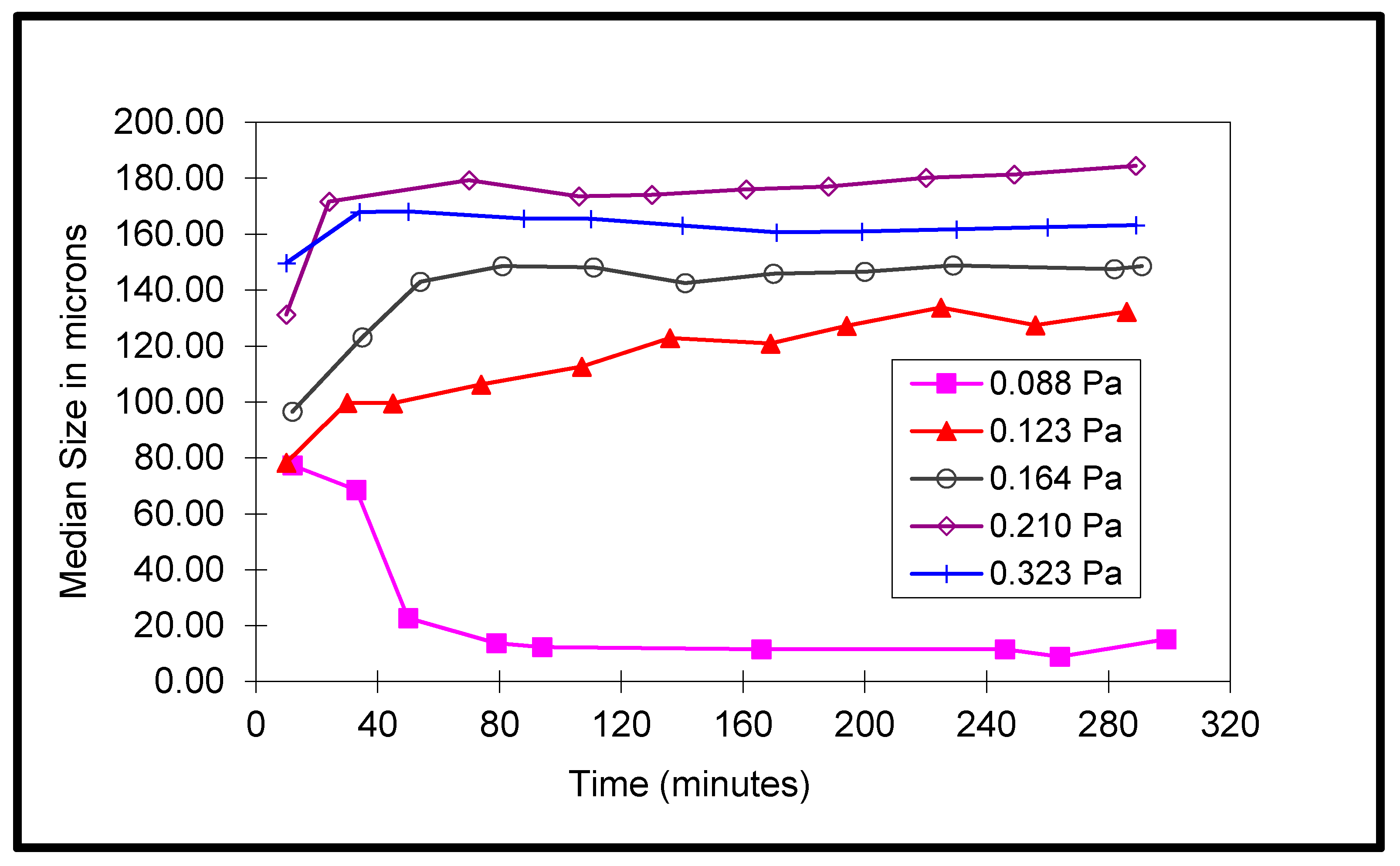
Size distribution data measured using the Malvern Particle Size Analyzer are summarized in Figure 12.
In Figure 12, the median sizes of the distributions are plotted as a function of time for different bed shear stresses. At the lowest shear stress (i.e., at 0.088 Pa), the median size decreases as a function of time. This means that the distributions are becoming finer and finer as the time progresses. This implies that larger flocs with higher settling velocities settle out, leaving the smaller flocs with lower settling velocities in suspension. Such a behavior is characteristics of particles settling as individual particles without interaction among particles. As the bed shear stress increases, a very different picture emerges. For example, for the bed shear stress of 0.123 Pa, the median size of the distributions shows an increasing trend with time, suggesting that the flocculation of sediment is taking place. For this and higher bed shear stresses, the median size increases initially with time and then it levels off towards a steady state value. The increase in the steady state median size of flocs does not continue monotonically as a function of the bed shear stress. It reaches a maximum value at a shear stress of 0.210 Pa. With a further increase in shear stress, the median size actually decreases. This is due to the fact that, at higher shear stresses, the flocs are breaking up due to high-intensity collisions due to turbulence.
The size distribution data clearly show the dual role of turbulence in the flocculation process. Turbulence promotes the formation of flocs initially, but as the intensity of turbulence increases, it starts to break up the flocs, suggesting that that there is an optimum level of turbulence that results in the maximum size of the flocs. The dual nature of turbulence becomes more evident when the full distributions are examined. In Figure 13, where the full distribution of sediment flocs are presented for bed shear stresses of 0.088, 0.210 and 0.323 Pa, the influence of the turbulence on flocculation is evident.
In Figure 13A, size distributions are shown for three different elapsed times, namely, zero minutes (initial distribution), 60 min and 120 min. The progressive fining of the sediment particles is evident due to the settlement of coarser fractions. Figure 13B shows the full distributions for the bed shear stress of 0.210 Pa. From Figure 13B, one can clearly see evidence of flocculation. At the elapsed time of 60 min, the percent volume of flocs in the size classes over 150 microns is considerably higher than the initial distribution of flocs in the same size range. This is a clear indication that the flocculation of the sediment particles has occurred. The same thing can also be said for the elapsed time of 120 min. Figure 13C shows the complete distribution of the flocs during deposition at the bed shear stress of 0.323 Pa. From this figure, one can see the evidence of floc breakage. The size of the largest floc that was formed during this experiment is about 390 microns, whereas for the lower bed shear stress experiment (0.210 Pa), the largest flocs formed were of the size of about 420 microns. Moreover, the percent by volume of the largest flocs were also lower for the higher bed shear stress run.
3.5. Determination of Cohesion Parameter β and Empirical Parameters B and C
The RIVFLOC model presented in Section 2.1 was tailored to the rotating circular flume, and the measured data from the rotating circular flume experiments were analyzed using this tailored model. Accordingly, the advection-dispersion equation for the rotating circular flume becomes:
where is the settling velocity of the kth size fraction, z is the vertical coordinate, t is the time axis and is the mass transfer coefficient. The flow in the rotating flume was considered to be two dimensional and the longitudinal variation was assumed to be negligible. Therefore, the mass balance equation took the simplified form of Equation (26) and the mass balance was considered only in the vertical direction. Boundary conditions at the sediment–water interface were exactly same as in the RIVFLOC model and the transport of sediment was treated in two stages, i.e., a transport stage and a flocculation stage, as was done in the RIVFLOC model. The flocculation module and the properties of flocs such as density and settling velocity of the sediment flocs were treated exactly the same way as in the RIVFLOC model.
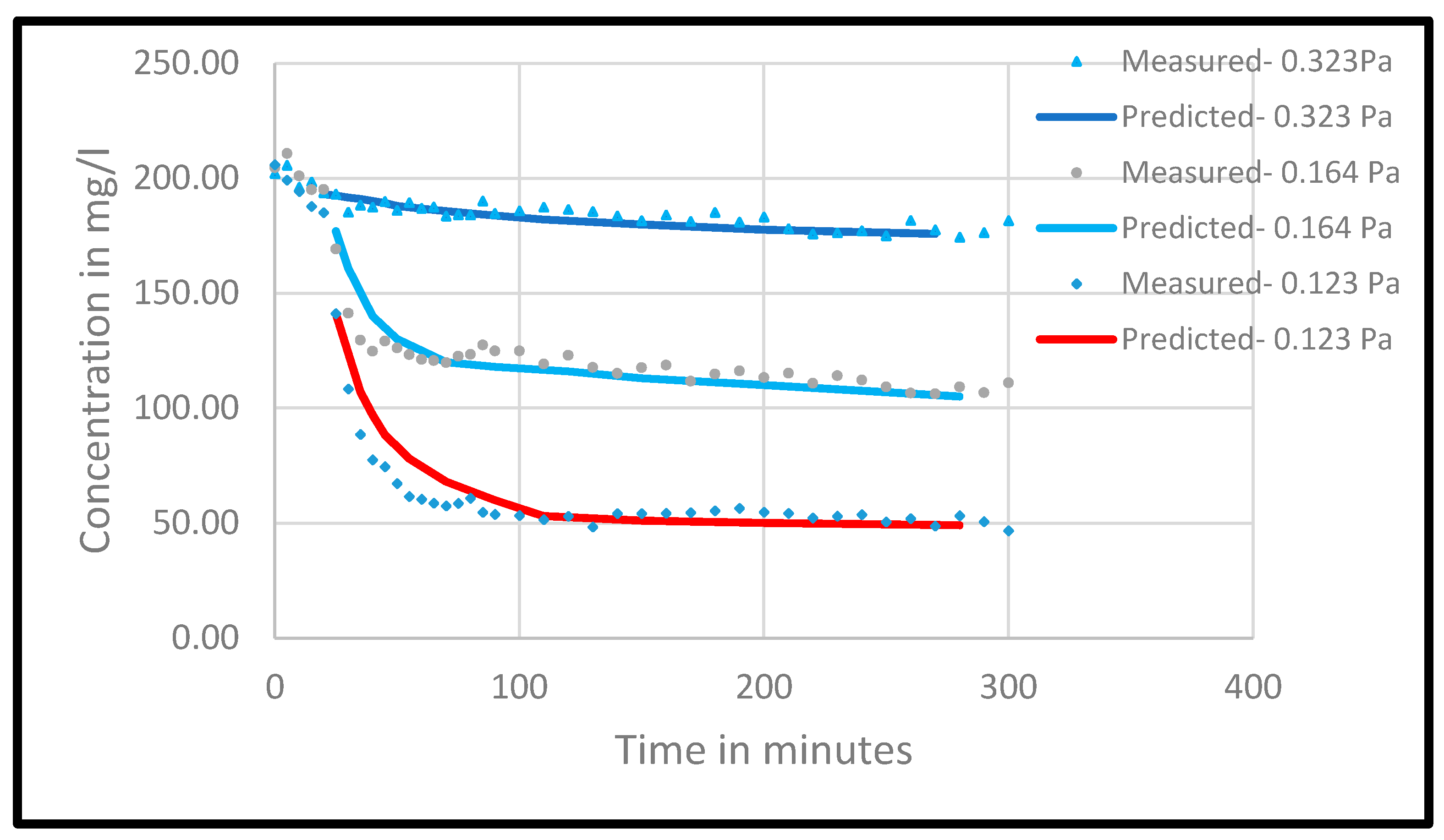
Results from the deposition experiments were analyzed using this model and a comparison between the model predictions and measurements are shown in Figure 14 for three different bed shear stress tests (0.323, 0.164, and 0.123 Pa).
In this analysis, the deposition test with the highest bed shear stress (0.323 Pa) was chosen for calibration, and the coefficients β, b and c were determined as part of the calibration process. The calibration was carried out using a trial-and-error procedure. To start the procedure, the values of b and c as given in Lau and Krishnappan [47] were chosen as the first approximation. Using the values of b and c, and using different values of β, the size distributions of the suspended flocs were determined using the model and the β value that gave the best agreement with the measured distributions was chosen. Using this chosen value of β, a range of b and c values were then tried in the model and the variation of concentration as a function of time was determined. This variation was then compared with the measured data and the set of values that gave the closest match was chosen. Then the process was repeated until the size distribution predictions and the concentration-time variation predictions agreed well with the measured data. Such a convergence was achieved within a limited number of iterations (usually within three). The values obtained for these parameters were as follows: b = 0.02, c = 1.35 and β = 0.010. The predicted concentration–time curves for the other two tests using the calibrated values for the parameters are plotted in Figure 14, and it can be seen from this figure that the agreement is good.
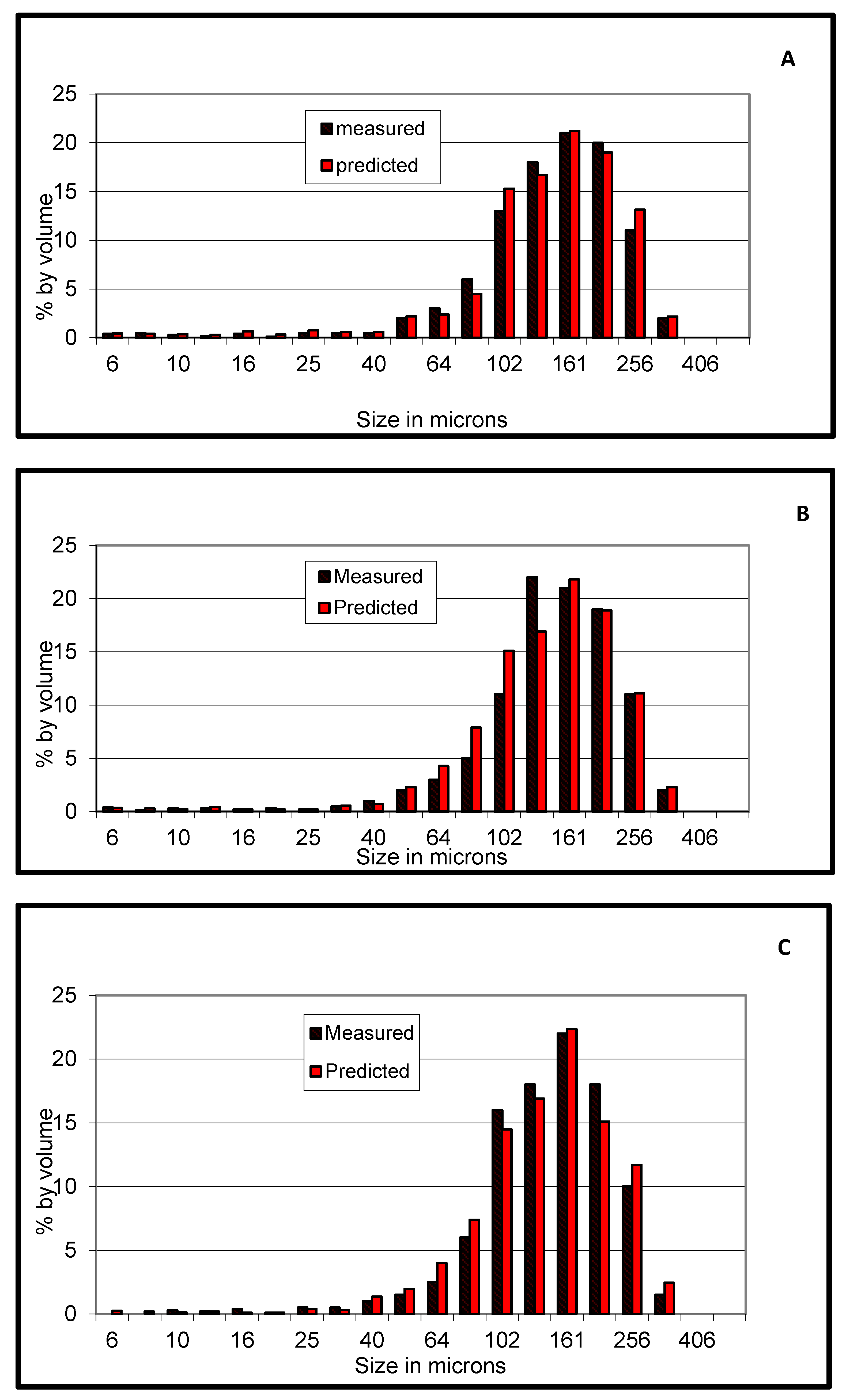
The comparisons of size distributions predicted and measured for the test (0.323 Pa) are shown in Figure 15. Figure 15A is for an elapsed time of 30 min from the start of the deposition experiments. It can be seen from this figure that the agreement between the predicted distributions and measured distribution is reasonable. Figure 15B,C are for elapsed times of 60 and 120 min, and both of these figures show a reasonable agreement between model predictions and the measured size distributions.
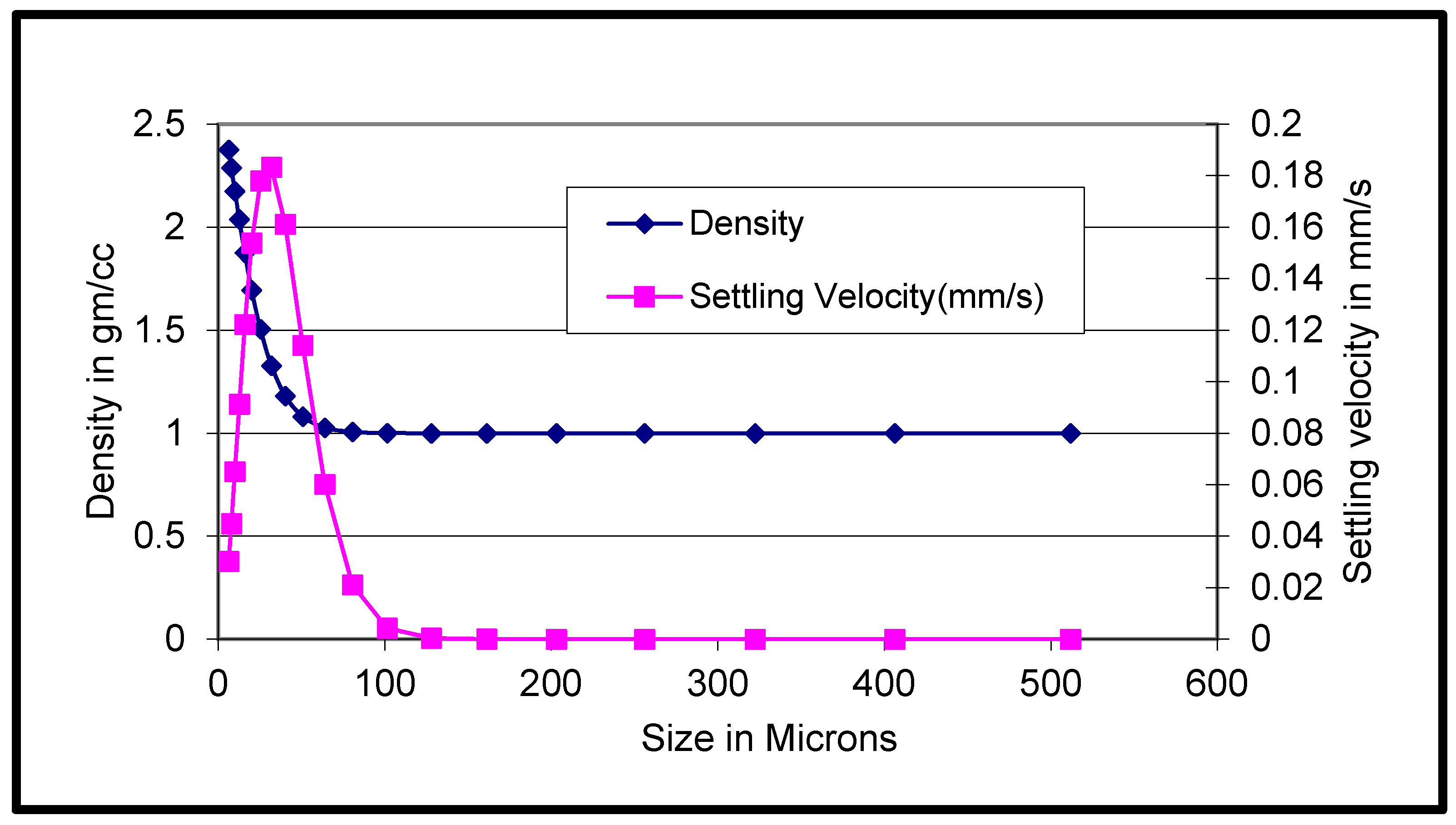
Knowing the empirical parameters b and c, density and settling velocity of the sediment flocs can be related to the size of the flocs as shown in Figure 16.
From Figure 16, one can see that the settling velocity of the flocs increases with the size of the flocs when the floc sizes are small, but after reaching a maximum value of about 0.18 mm/s, settling velocity actually decreases with the increase in floc sizes and it approaches zero for larger floc sizes. This is because the effective density is close to that of water for larger flocs. Size distribution data also support this observation. The size distribution of flocs that stayed in suspension were large and the effective density tending towards that of the suspending medium. An inverse relationship between the settling velocity and the size of flocs for larger flocs was also observed by other investigators [61,62].
3.6. Review of the Variability of Model Parameters
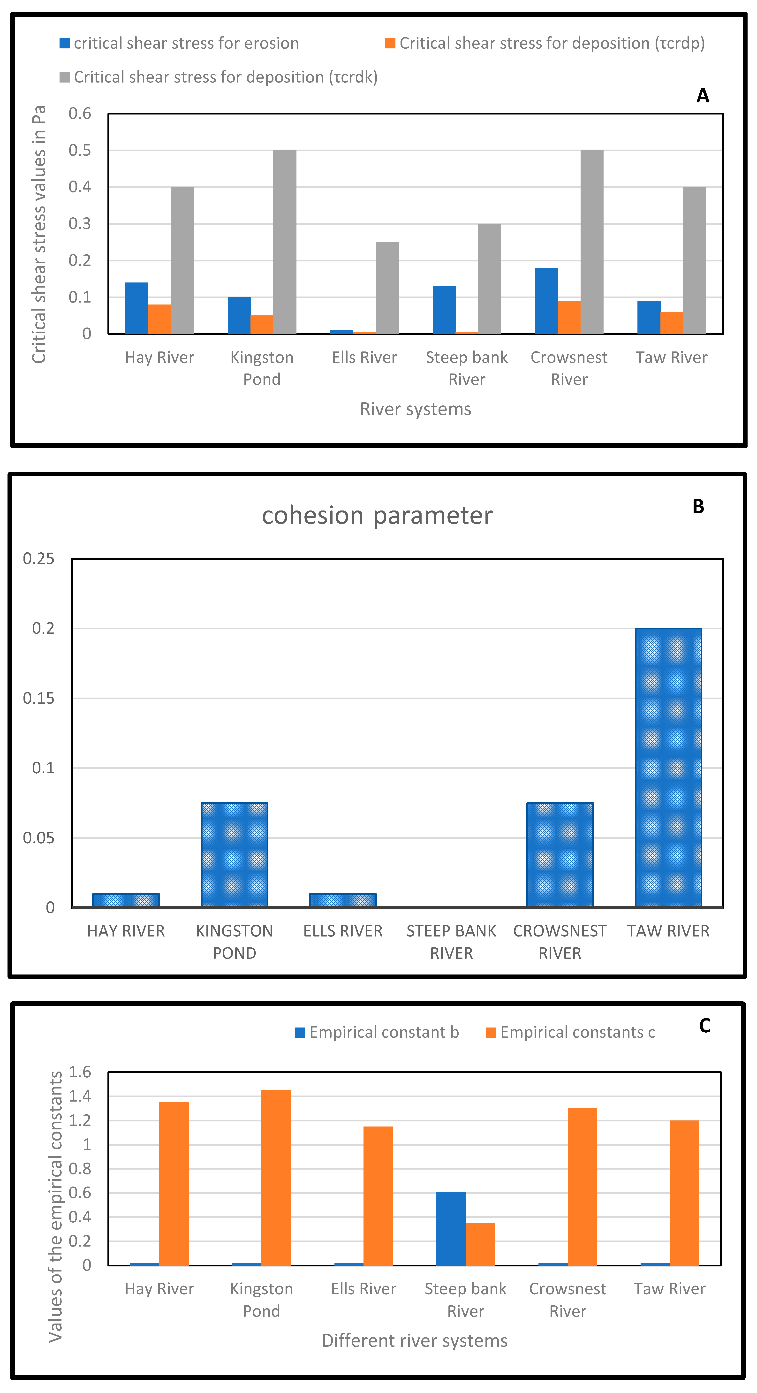
The variability of the model parameters among different river systems summarized in Table 2 is reviewed here in Figure 17.
Figure 17A shows the variability of the critical shear stress for erosion and the critical shear stresses for deposition () for all the river systems. From Figure 17A, one can see that the critical shear stress for erosion is always higher than the critical shear stress for deposition (Partheniades definition, ) because the sediment depositing to the bed gets attached to the sediment in the bed due to cohesion and a higher stress is needed to dislodge the deposited particle. It can also be seen from Table 3 and Figure 17A that there is about 10-fold variation in the values of both critical shear stress for erosion and the critical shear stress for deposition (Partheniades definition,) for the river systems. The critical shear stress for deposition (Krones definition, varies from 0.25 to 0.50 Pa and it is much higher than the critical shear stress for deposition (Partheniades definition, ). The proportions of these three stresses in each river system are different and point to the need for testing site-specific sediments in the flume in order to achieve a reasonable accuracy in model predictions.
Figure 17B shows the variability of the cohesion parameter, β, for the various river systems. Cohesion parameter is a measure of the efficiency of the system to flocculate for a given number of particle collisions. The variability of the cohesion parameter is in the of range of 0 to 0.1 except for the Taw River system for which the cohesion parameter is 0.20. The high value of the cohesion parameter for the Taw River system is due to the fact that it drains an organic rich peaty and podzolic moorland soils near its source and clayey gley and brown earth soils in more intensely formed lowland adjacent to the moor. Cohesion parameter variability also demonstrates the need for site-specific sediment testing in flumes for reliable predictions from models.
From Figure 17C, one can see that the variability in the empirical constants b and c are not high except for the Steepbank River for which the values of the constants are reversed, suggesting that the relationship between the floc sizes and density is very different for the Steepbank River in comparison to the other river systems. Indeed, if one examines the settling velocity relationship with floc sizes for different river systems, one can see that the relationship for the Steepbank River is very different. The settling velocity vs. the floc size relationships are plotted in Figure 18.
Figure 18 shows that the settling velocity variation as a function of floc sizes is similar for sediment from different river systems except for the Steepbank River. The Steepbank River, which is located in the Athabasca Oil Sands region in Alberta, is impacted by the oil sands development. The river flows through the bituminous soils and hence the sediment in the river is coated with bitumen and consequently becomes hydrophobic. As a result, the sediment flocs are tightly bound and have a higher density and behave like cohesionless sediment without much flocculation. In fact, the cohesion parameter for this sediment is zero. Such variability in modelling parameters also points to the need for testing site-specific sediments to obtain reliable predictions of transport models.
3.7. Importance of the Entrapment Process
In most of the river systems for which the RIVFLOC model was applied (i.e., the river systems listed in Table 2), the bed shear stresses were one to two orders of magnitude higher than the critical shear stress for deposition ( Krone’s definition), and therefore the deposition flux specified to the model is zero (see Equation (3)), which means that the fine sediment entering a river system will be transported as a plug flow without any deposition to the river beds. However, the sampling of the bed materials in some of these rivers does show evidence of fine sediment presence in these beds [63]. Size fractions of fine sediment found in these beds do overlap with the sizes fractions of sediment found in suspension. The presence of fine sediment in the bed is attributed to the process of entrapment in which the fine sediment ingresses into the interstitial voids of the bed sediment as the sediment–water mixture flows through the bed sediment matrix due to infiltration. The cohesion property of the fine sediment causes the fine sediment to stick to the bed matrix [16,17]. Krishnappan and Engel [43] studied the entrapment process using the rotating circular flume and found that the deposition of fine sediment can occur at bed shear stresses much larger than the critical shear stress for deposition, .
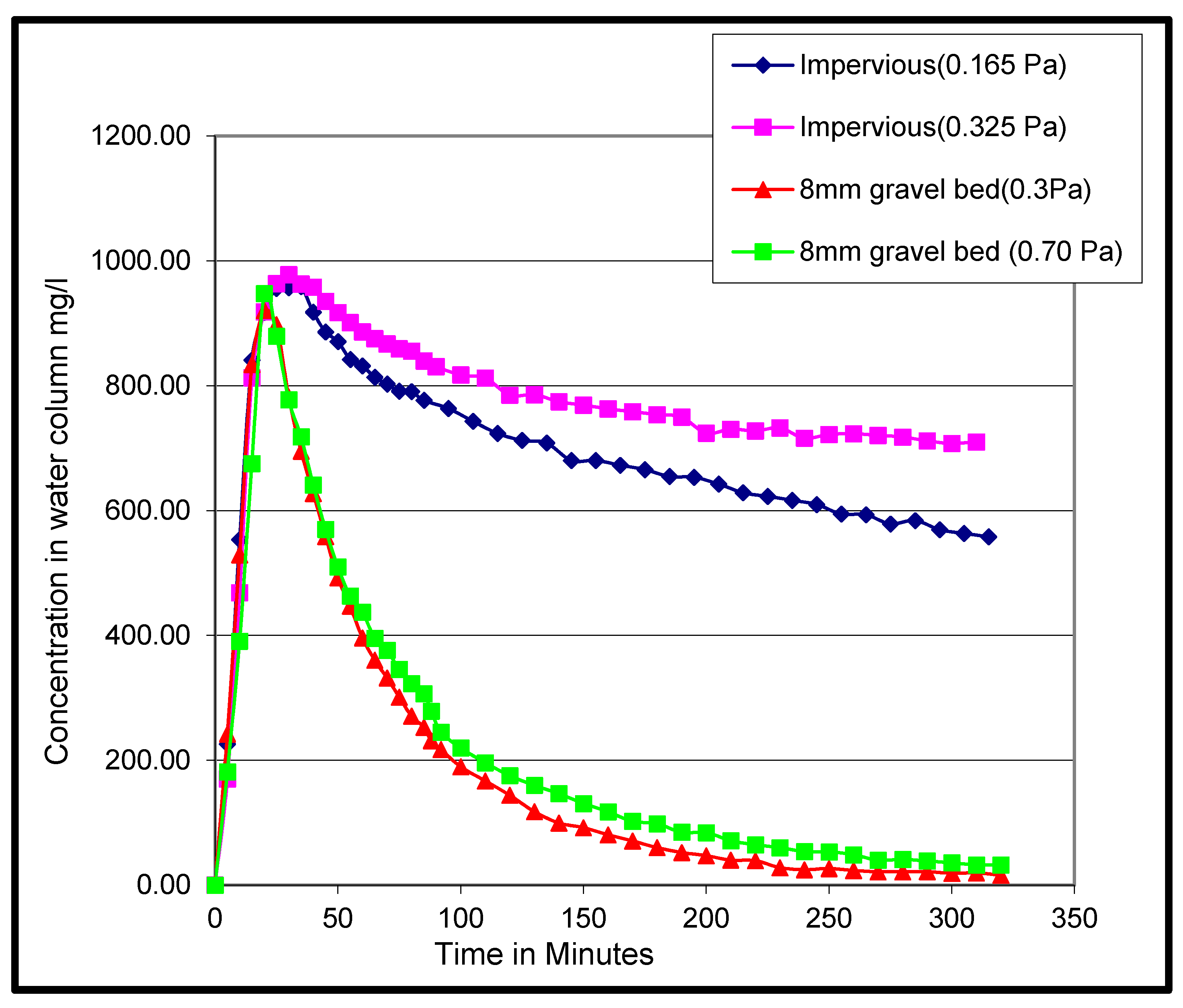
Figure 19 shows results from the entrapment experiments carried out by Krishnappan and Engel [43]. In these experiments, kaolin was used as a surrogate for fine sediment, and deposition experiments were conducted for two different bed conditions, namely, a plane, impervious bed and a bed covered with 8 mm gravel. Two different bed shear stresses were tested for each configuration (0.165 and 0.325 Pa for impervious runs and 0.30 and 0.70 Pa for gravel bed runs). The concentration variations as a function of time measured for these tests are shown in Figure 19. From Figure 19, one can see that the time variation of concentration profiles of impervious bed runs is significantly different from those of gravel bed runs. Note that when the bed is covered with gravel, almost all of the initially suspended material was entrapped into the voids of the gravel and the concentration of sediment in suspension was nearly zero. When the bed was impervious (smooth flume bed), the sediment stayed mainly in suspension and the deposition rates were considerably smaller (judging by the slope of the concentration decay curves). The bed shear stress value of 0.70 Pa is higher than the critical shear stress for the deposition of kaolin (), which was estimated to 0.50 Pa.
Krishnappan and Engel [43] modelled the entrapment of kaolin in the gravel bed using the RIVFLOC model tailored to the rotating flume and found that the coefficient of entrapment varied from 0.19 to 0.94. No attempt was made in that study to relate the coefficient of entrapment to bulk properties of the bed such as the porosity of the gravel substrate, thickness of the gravel bed and the permeability.
Glasbergen [64] studied the entrapment process using the rotating circular flume for fine sediment and coarse gravel from the Elbow River in Alberta. He evaluated the coefficient of entrapment using the method of Krishnappan and Engel [43] and obtained a value of 0.20 for the coefficient. He too did not make any attempt to relate the coefficient of entrapment to the bulk properties of the river-bed materials. Therefore, there is a need for further research in this area to have a better understanding of the entrapment process, which is crucial for modelling the fate of the fine sediments and the associated contaminants.
Fine sediment that is entrapped in coarse gravel beds remain in the bed until the coarse sediment beds are eroded, which is likely under high flows. The initiation of the movement of the coarse gravel can be predicted reliably using the Shield’s diagram for critical shear stress for the erosion of coarse-grained sediment.
4. Discussion
The model parameters obtained by the application of the RIVFLOC model to the rotating flume experiments for different river systems lead to some interesting observations. For example, the cohesion parameter obtained for the Taw River system in the UK is about two to three times higher than the values obtained for the other river systems. As indicated earlier, cohesion parameter reflects the efficiency of collisions in the formation of flocs. This means that, for the Taw River sediment, more collisions will result in the formation of flocs. This can be attributed to the organic matter content of the sediment. Indeed, Taw River flows through an organic rich peaty and podzolic moorland near its source and an intensely farmed lowland downstream.
The empirical constants determined for different river systems enable the calculation of settling velocities as a function of floc sizes as shown in Figure 18. From this figure, the maximum settling velocity and the flocs size corresponding to the maximum settling velocity (optimum floc size) are extracted and summarized in Table 3.
From Table 3, one can see that the Ells River sediment has the maximum settling velocity of 0.37 mm/sec and the optimum floc size of 51 microns compared to all other sediments. It is interesting to note that the Taw River sediment, which has the highest cohesion parameter, is not the one with the highest settling velocity and the largest optimum floc size. Efficiency in flocculation does not imply that the resulting flocs will have the largest floc size and the highest settling velocity. The high settling velocity and the large optimum floc size of the Ells River may be attributed to the river basin, which is a tar-sand region with a high percentage of bituminous coal content.
The lowest settling velocity and the smallest optimum floc size corresponds to the sediment in the Kingston storm water pond, which is an in-stream pond with lower bed shear stresses over a large area of the pond. There is substantial deposition of sediment in the pond and the sediment in suspension are finer with lower settling velocities.
The Steepbank River sediments show an interesting behavior. The sediment in this river behaves as a cohesionless sediment with practically no flocculation (the cohesion parameter for this sediment is zero) and the settling velocity shows a monotonic increase with the size of the sediment. It should be noted that the Steepbank River basin is also in the tar sand region, but it is highly impacted by the operation of the Fort McMurray tar sands oil development project. The Ells River basin, on the other hand, is not impacted by this project.
One of the major difficulties in carrying out the laboratory investigation of the cohesive sediment transport processes involves the transportation of a large volume of river water and sediment mixture (about 500 to 1000 L) from the river site to the laboratory flume. For river sites in Canada, it was possible to transport such large volume of samples in transport trucks fitted with refrigerated storage containers. For the Taw River study, river water was not used because of the cost of transportation, and hence the local tap water was used to carry out the tests. The impact of the tap water use instead of river water was not addressed in this study.
Another source of error that might have had an effect on the sediment behavior is the lack of temperature control for the rotating flume. The rotating flume experiments were carried out in room temperature after the sediment–water mixtures were placed in the flume. Prior to that, the samples were stored in the refrigerator maintained at 4 degrees centigrade. Lack of temperature control could have had an effect on the bacterial growth during the conduct of experiments in the rotating flume.
Error estimates in the determination of model parameters were not made in the reviewed studies. There is a degree of human judgement involved in the determination of the critical conditions at which the erosion and deposition of sediment is occurring and how the calculated distributions agree with the measured distributions to determine the empirical constants and cohesion parameter. The methods employed in these studies were aimed to reduce the human judgement in establishing these model parameters. The measurement of sediment concentrations and bed shear stresses were also carried out with a high degree of precision (within ±1 mg/L and ±0.001 Pa).
5. Conclusions
A semi-empirical modelling technique for the transport of cohesive sediment is needed because of the large number of controlling parameters governing the erosion and deposition of cohesive sediments and the flocculation process that distinguishes the fine sediment from the cohesionless coarse-grained sediment for which there are well established models available in the literature. An examination of the details of a semi-empirical cohesive sediment transport model called RIVFLOC highlights the model parameters that needed to be determined using a rotating circular flume. The parameters that were determined using the rotating circular flume include the critical shear stress for erosion of the cohesive sediment, critical shear stress for deposition according to the definition of Partheniades, critical shear stress for deposition according to the definition of Krone, the cohesion parameter governing the flocculation of cohesive sediment and two empirical parameters that define the density of the floc in terms of the size of the flocs.
The critical shear stress for the erosion of cohesive sediment is different from the critical shear stress for deposition, suggesting that the cohesive sediments do not undergo erosion and deposition simultaneously, unlike the cohesionless sediment for which the two critical conditions coincide and the sediment undergoes simultaneous erosion and deposition. The flocculation of the cohesive sediment was inferred from the measurement of the size distribution of sediment flocs using a sizing instrument, which shows that the cohesive sediment did indeed flocculate. The density of the flocs is dependent on the size of the flocs; as the size of the floc increases, more of the surrounding fluid is incorporated in the structure of the floc. An empirical equation relates the floc density with floc size, which in turn provides a relationship for the settling velocity based on the Stokes equation.
The semi-empirical RIVFLOC model was applied to a number of river systems to model the transport of cohesive sediments and associated contaminants. The various model parameters determined for these river systems were compared and the variability in the model parameters were examined. The variabilities in these parameters suggest that the establishment of model parameters for site-specific sediment is important for accurate predictions of the cohesive sediment transport models.
Application of the RIVFLOC model to various river systems points to the need for modelling the entrapment process of cohesive sediment transport. The entrapment process is responsible for the presence of fine sediment in coarse-grained sediment bed matrix in gravel bed rivers where the bed shear stress far exceeds the critical shear stress for deposition, as defined by Krone. More research is needed to relate the coefficient of entrapment with the bulk properties of coarse-grained sediment bed matrix.
Funding
This research received no external funding.
Institutional Review Board Statement
This study was conducted in accordance with the Declaration of Helsinki.
Informed Consent Statement
Not applicable.
Data Availability Statement
Data supporting reported results can be requested from the author.
Conflicts of Interest
The authors declare no conflict of interest.
References
- Raudkivi, A.J. Loose Boundary Hydraulics, 4th ed.; Balkema, A.A., Ed.; CRC Press: Boca Raton, FL, USA.
- Van Leussen, W. Aggregation of Particles, Settling Velocity of Mud Flocs. In Physical Processes in Estuaries; Van Leussen, D., Ed.; Springer: New York, NY, USA, 1988. [Google Scholar]
- Partheniades, E. A study of erosion and deposition of cohesive soils in salt water. Ph.D. Thesis, University of Florida, Gainesville, FL, USA, 1962. [Google Scholar]
- Partheniades, E. Results of recent investigation on erosion and deposition of cohesive sediments. In Sedimentation; Shen, H.W., Ed.; Colorado State University: Fort Collins, CO, USA, 1972. [Google Scholar]
- Partheniades, E. The present state of knowledge and needs for future research on cohesive sediment dynamics. In River Sedimentation, Proceedings of the 3rd International Symposium; Wang, S.Y., Shen, H.W., Ding, L.Z., Eds.; School of Engineering, University of Mississippi: Jackson, MS, USA, 1986; Volume 3, pp. 3–25. [Google Scholar]
- Partheniades, E.; Kennedy, J.F. Depositional behaviour of fine sediments in a turbulent fluid motion. In Proceedings of the 10th Conference on Coastal Engineering, London, UK, 1–5 September 1966; American Society of Civil Engineers: New York, NY, USA, 1966; Volume 2, pp. 707–724. [Google Scholar]
- Patheniades, E.; Cross, R.H.; Arora, A. Further results on the deposition of cohesive sediments. In Proceedings of the 11th Conference on Coastal Engineering, London, UK, 16–20 September 1968; American Society of Civil Engineers: New York, NY, USA, 1968; Volume 2, pp. 723–742. [Google Scholar]
- Einstein, H.A.; Anderson, A.G.; Johnson, J.W. A distinction between bed-load and suspended load in natural streams. Trans. Am. Geophys. Union 1940, 21, 628–633. [Google Scholar] [CrossRef]
- Einstein, H.A. The Bed Load Function for Sediment Transportation in Open Channel Flows; Technical Bulletin No. 1026; U.S. Department of Agriculture, Soils Conservation Service: Washington, DC, USA, 1950.
- Yalin, M.S. Mechanics of Sediment Transport, 1st ed.; Pergamon Press: Braunschweig, Germany, 1972. [Google Scholar]
- Krone, R.B. Flume Studies of Transport of Sediment in Estuarial Shoaling Processes: Final Report; Hydraulic Engineering Laboratory and Sanitary Engineering Research Laboratory, University of California: Berkeley, CA, USA, 1962. [Google Scholar]
- Mehta, A.J.; Partheniades, E. An Investigation of the Depositional Properties of Flocculated Fine Sediments. J. Hydraul. Res. 1975, 13, 361–381. [Google Scholar] [CrossRef]
- Lick, W. Entrainment, deposition and transport of fine grained sediments in Lakes. Hydrobiologia 1982, 91, 31–40. [Google Scholar] [CrossRef]
- Krishnappan, B.G.; Engel, P. Critical shear stresses for erosion and deposition of suspended sediments of the Fraser River. In Cohesive Sediments; Burt, N., Parker, R., Watts, J., Eds.; John Wiley and Sons: Chichester, UK, 1997; pp. 279–288. [Google Scholar]
- Krishnappan, B.G.; Marsalek, J. Chapter 8: An example of modelling flocculation in a freshwater aquatic system. In Flocculation in Natural and Engineered Environmental Systems; Droppo, I., Leppard, G.G., Liss, S.N., Mulligan, T.G., Eds.; CRC Press: Boca Raton, FL, USA, 2005; pp. 171–188. [Google Scholar]
- Packman, A.I.; Brooks, N.H.; Morgan, J.J. Physico-chemical model for colloid exchange between a stream and a sand stream bed with bedforms. Water Resour. Res. 2000, 36, 2351–2361. [Google Scholar] [CrossRef]
- Packman, A.I.; Brooks, N.H.; Morgan, J.J. Kaolinite exchange between a stream and stream bed: Laboratory experiment and validation of a colloidal transport model. Water Resour. Res. 2000, 36, 2363–2372. [Google Scholar] [CrossRef]
- Owen, M.W. A Detailed Study of Settling Velocities of an Estuarine Mud; Report INT78; Hydraulic Research Station: Wallingford, UK, 1970. [Google Scholar]
- Ongley, E.D.; Bynoe, M.C.; Percival, J.B. Physical and geochemical characteristics of suspended solids, Wilton Creek, Ontario. Can. J. Earth Sci. 1981, 18, 1365–1379. [Google Scholar] [CrossRef]
- Droppo, I.G.; Ongley, E.D. Flocculation of suspended solids in Southern Ontario rivers. Water Res. 1994, 28, 1799–1809. [Google Scholar] [CrossRef]
- Droppo, I.G.; Leppard, G.G.; Liss, S.N.; Milligan, T.G. Chapter 20: Opportunities, Needs and Strategic Direction for Research on Flocculation in Natural and Engineered Systems. In Flocculation in Natural and Engineered Environmental Systems; Droppo, I., Leppard, G.G., Liss, S.N., Mulligan, T.G., Eds.; CRC Press: Boca Raton, FL, USA, 2005; pp. 407–421. [Google Scholar]
- Rao, S.S.; Droppo, I.G.; Taylor, C.M.; Burnison, B.K. Fresh Water Bacterial Aggregate Development: Effects of Dissolved Organic Matter; NWRI Contribution 91–75; National Water Research Institute, CCIW: Burlington, ON, Canada, 1991. [Google Scholar]
- Leppard, G.G. Evaluation of electron microscope techniques for the description of aquatic colloids. In Environmental Particles; Buffle, J., Van Leeuwen, H.P., Eds.; IUPAC Environmental and Analytical Chemistry Series; Lewis Publishers: Boca Raton, FL, USA, 1992; Volume 1, pp. 231–289. [Google Scholar]
- Ruehrwein, R.A.; Ward, D.W. Mechanism of clay aggregation by polyelectrolytes. Soil Sci. 1952, 73, 485–492. [Google Scholar] [CrossRef]
- La Mer, V.K.; Heley, T.W. Adsorption-flocculation reactions of macromolecules at the solid-liquid interfaces. Rev. Pure Appl. Chem. 1963, 13, 112–132. [Google Scholar]
- Busch, P.L.; Stumm, W. Chemical interactions in the aggregation of bacteria: Bio-flocculation in waste treatment. Environ. Sci. Technol. 1968, 2, 49–53. [Google Scholar] [CrossRef]
- Ariathurai, R.; Arulanandan, K. Erosion rates of cohesive soils. J. Hydraul. Div. ASCE 1978, 104, 279–283. [Google Scholar] [CrossRef]
- Lee, D.-Y.; Lick, W.; Kang, S.W. The Entrainment and Deposition of Fine-Grained Sediments in Lake Erie. J. Great Lakes Res. 1981, 7, 224–233. [Google Scholar] [CrossRef]
- Dixit, J.G. Resuspension Potential of Deposited Kaolinite Beds. Master’s Thesis, University of Florida, Gainesville, FL, USA, 1982. [Google Scholar]
- Parchure, T.M. Erosional Behaviour of Deposited Cohesive Sediments. Ph.D. Thesis, University of Florida, Gainesville, FL, USA, 1984. [Google Scholar]
- Krishnappan, B.G. Erosion behaviour of fine sediment deposits. Can. J. Civ. Eng. 2004, 31, 759–766. [Google Scholar] [CrossRef]
- Hayter, E.J. Finite Element Hydrodynamic and Cohesive Sediment Transport Modelling System; Department of Civil Engineering, Clemson University: Clemson, SC, USA, 1987. [Google Scholar]
- Krishnappan, B.G. Modelling of cohesive sediment transport. In Proceedings of the International Symposium on the Transport of Suspended Sediment and its Mathematical Modelling, Florence, Italy, 2–5 September 1991. [Google Scholar]
- Krishnappan, B.G. Cohesive sediment transport studies using a rotating circular flume. In Proceedings of the 7th International Conference on Hydro-Science and Engineering (ICHE-2006), Philadelphia, PA, USA, 10–13 September 2006. [Google Scholar]
- Krishnappan, B.G.; Marsalek, J. Modelling of flocculation and transport of cohesive sediment from an on-stream stormwater detention pond. Water Res. 2002, 36, 3849–3859. [Google Scholar] [CrossRef]
- Droppo, I.G.; Krishnappan, B.G. Modeling of hydrophobic cohesive sediment transport in the Ells River Alberta, Canada. J. Soils Sediments 2016, 16, 2753–2765. [Google Scholar] [CrossRef]
- Krishnappan, B.G. Personal Communication; Krishnappan Environmental Consultant: Hamilton, ON, Canada, 2015. [Google Scholar]
- Stone, M.; Krishnappan, B.G.; Silins, U.; Emelko, M.B.; Williams, C.H.S.; Collins, A.L.; Spencer, S.A. A new framework for modelling fine sediment transport in rivers includes flocculation to inform reservoir management in wildfire impacted watersheds. Water 2021, 13, 2319. [Google Scholar] [CrossRef]
- Stone, M.; Krishnappan, B.G.; Granger, S.; Upadhayay, H.R.; Zhang, Y.; Chivers, C.A.; Decent, Q.; Collins, A.L. Deposition behaviour of cohesive sediment in the upper Taw observatory, Southern UK: Implications for management and modelling. J. Hydrol. 2021, 598, 126145. [Google Scholar] [CrossRef]
- Yotsukura, N.; Sayre, W.W. Transverse mixing in natural channels. Water Resour. Res. 1976, 12, 695–704. [Google Scholar] [CrossRef]
- Mehta, A.J.; Partheniades, E. Resuspension of deposited cohesive sediment beds. In Proceedings of the 18th Coastal Engineering Conference, Cape town, South Africa, 14–19 November 1982; Edge, B.L., Ed.; ASCE: New York, NY, USA, 1983; Volume 2, pp. 1569–1588. [Google Scholar]
- Krishnappan, B.G.; Stone, M.; Granger, S.J.; Upadhayay, H.R.; Tang, Q.; Zhang, Y.; Collins, A.L. Experimental investigation of erosion characteristics of fine grained cohesive sediments. Water 2020, 12, 1511. [Google Scholar] [CrossRef]
- Krishnappan, B.G.; Engel, P. Entrapment of fines in coarse sediment beds. In River Flow 2006; Ferrira, A., Leal, C., Eds.; Taylor and Francis Group: London, UK, 2006; pp. 817–824. [Google Scholar]
- Stone, H.L.; Brian, P.L.T. Numerical solution of convective transport problems. Am. Inst. Chem Eng. J. 1963, 9, 681–688. [Google Scholar] [CrossRef]
- Krishnappan, B.G.; Lau, Y.L. RIVMIX MK2: User Manual; Hydraulics Division, National Water Research Institute: Burlington, ON, Canada, 1985; p. 25. [Google Scholar]
- Fuchs, N.A. Mechanics of Aerosols; Pergamon: New York, NY, USA, 1964; p. 408. [Google Scholar]
- Lau, Y.L.; Krishnappan, B.G. Measurement of Size Distribution of Settling Flocs; NWRI Contribution No. 97–223; Environment Canada: Burlington, ON, Canada, 1997; p. 21.
- Valioulis, I.A.; List, E.J. Numerical simulation of a sedimentation Basin. 1. Model Development. Environ. Sci. Technol. 1984, 18, 242–247. [Google Scholar] [CrossRef]
- Tambo, N.; Watanabe, Y. Physical aspects of flocculation process—I: Fundamental Treatise. Water Res. 1979, 13, 429–439. [Google Scholar] [CrossRef]
- Djordjevic, S. Mathematical model of unsteady transport and its experimental verification in a compound open channel flow. J. Hydraul. Res. 1993, 31, 229–248. [Google Scholar] [CrossRef]
- Guan, Y.; Altinakar, M.S.; Krishnappan, B.G. Modelling of lateral flow distribution in compound channels. In Proceedings of the River Flow 2002 International Conference on Fluvial Hydraulics, Louvan-la Neuve, Belgium, 4–6 September 2002. [Google Scholar]
- Krishnappan, B.G. User Manual: Unsteady, Non-Uniform Mobile Boundary Flow Model—MOBED; Hydraulics Division, National Water Research Institute: Burlington, ON, Canada, 1981; p. 197. [Google Scholar]
- Krishnappan, B.G. MOBED User Manual Update I.; Hydraulics Division, National Water Research Institute: Burlingtom, ON, Canada, 1983; p. 72. [Google Scholar]
- Krishnappan, B.G. MOBED User Manual Update II.; Hydraulics Division, National Water Research Institute: Burlingtom, ON, Canada, 1986; p. 95. [Google Scholar]
- Krishnappan, B.G. Rotating Circular Flume. J. Hydraul. Eng. ASCE 1993, 119, 658–667. [Google Scholar] [CrossRef]
- Krishnappan, B.G.; Engel, P.; Stephens, R. Shear Velocity Distribution in a Rotating Flume; NWRI Contribution No. 94–102; NWRI: Burlington, ON, Canada, 1994. [Google Scholar]
- Petersen, O.; Krishnappan, B.G. Measurement and analysis of flow characteristics in a rotating circular flume. J. Hydraul. Res. IAHR 1994, 32, 483–494. [Google Scholar] [CrossRef]
- Krishnappan, B.G.; Engel, P. Distribution of bed shea stress in a rotating circular flume. J. Hydraul. Eng. ASCE 2004, 130, 324–331. [Google Scholar] [CrossRef]
- Rosten, H.I.; Spalding, D.B. The PHOENICS Reference Manual, TR/200; CHAM Ltd.: London, UK, 1984. [Google Scholar]
- Weiner, B.B. Particle and droplet sizing using Fraunhofer Diffraction. In Modern Method of Particle Size Analysis; Bath, H.G., Ed.; John Wiley and Sons: London, UK, 1984; Chapter 5. [Google Scholar]
- Petticrew, E.L. The composite nature of suspended and gravel stored fine sediments in streams: A case study of O’Ne-eil Creek, British Columbia, Canada. In Flocculation in Natural and Engineered Environmental Systems; Droppo, I.G., Leppard, G.G., Liss, S.N., Milligan, T.G., Eds.; CRC Press: Boca Raton, FL, USA, 2005; pp. 71–93. [Google Scholar]
- Atkinson, J.F.; Chakraborti, R.K.; VanBenschoten, J.E. Effect of floc size and shape in particle aggregation. In Flocculation in Natural and Engineered Environmental Systems; Droppo, I.G., Leppard, G.G., Liss, S.N., Milligan, T.G., Eds.; CRC Press: Boca Raton, FL, USA, 2005; pp. 95–120. [Google Scholar]
- Suzanne, C.L. Effects of Natural and Anthropogenic Non-Point Source Disturbances on the Structure and Function of Tributary Ecosystems in the Athabasca Oil Sands Region. Master’s Thesis, University of Victoria, Victoria, BC, Canada, 2015. [Google Scholar]
- Glasbergen, K.A. The Effect of Coarse Gravel on Cohesive Sediment Entrapment. Master’s Thesis, University of Waterloo, Waterloo, ON, Canada, 2013. [Google Scholar]
Figure 1.
The curvilinear co-ordinate system used in RIVFLOC model.

Figure 2.
Schematic representation of flocculation stage.
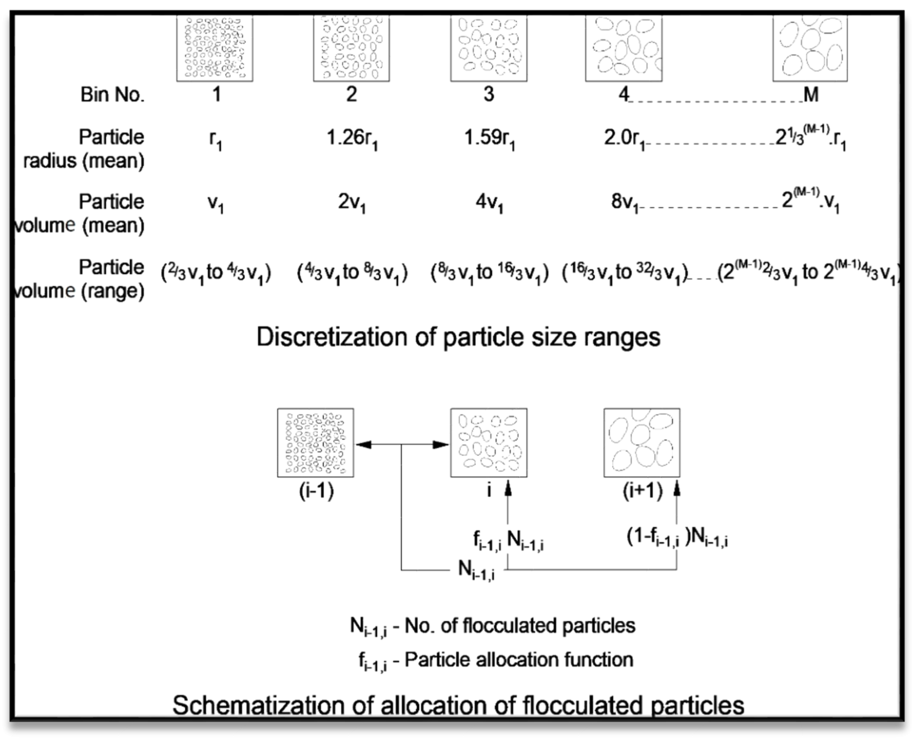
Figure 3.
A photograph of the top view of the rotating circular flume.

Figure 4.
Bed shear stress distribution as a function of distance along the flume width.
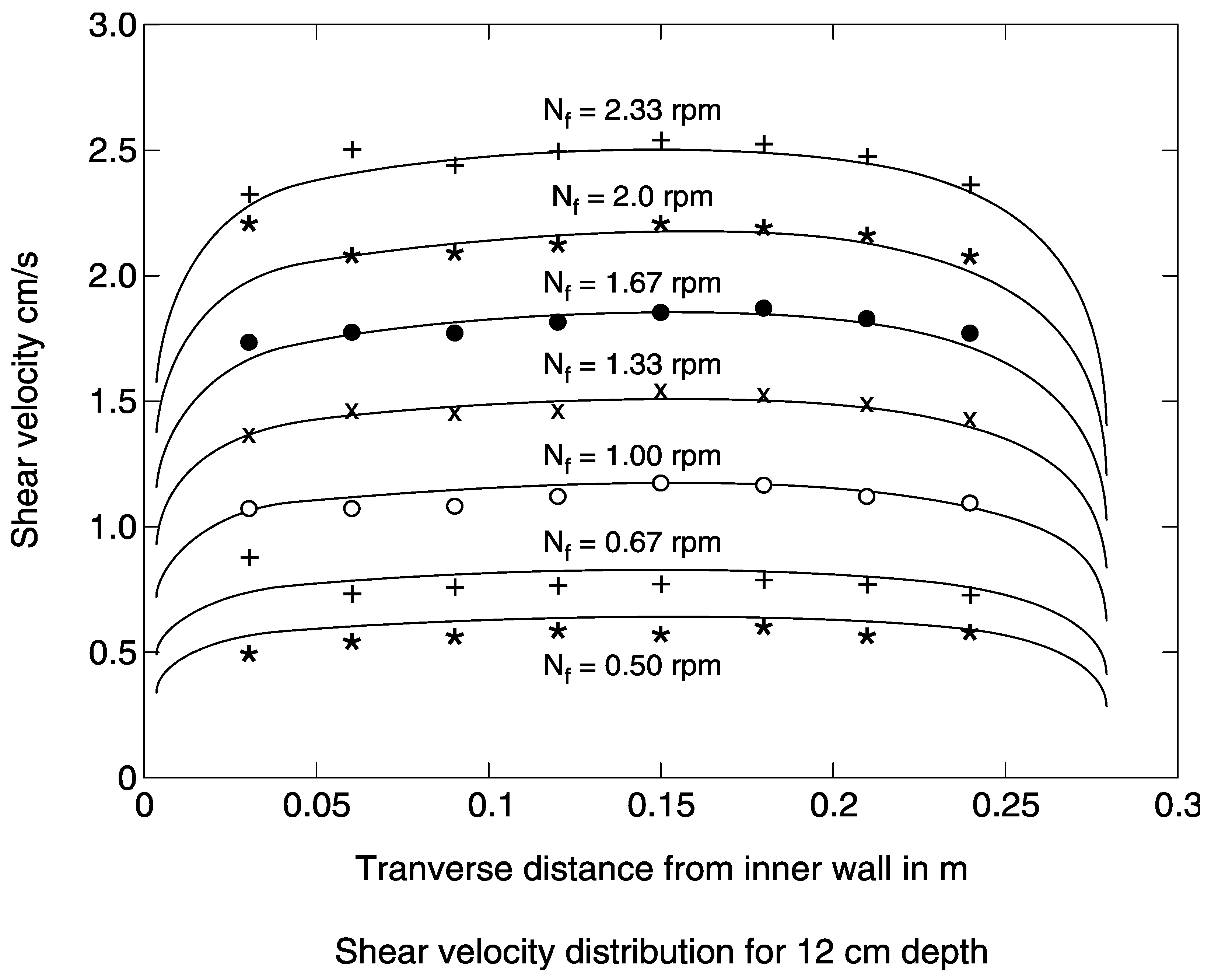
Figure 5.
Schematic diagram showing the arrangement of the particle size analyzer mounted on the flume.
Figure 5.
Schematic diagram showing the arrangement of the particle size analyzer mounted on the flume.

Figure 6.
A photograph showing the placement of the Malvern instrument underneath the flume.

Figure 7.
Inverted cone sampler for collecting samples of sediment–water mixture for testing in rotating circular flume.
Figure 7.
Inverted cone sampler for collecting samples of sediment–water mixture for testing in rotating circular flume.
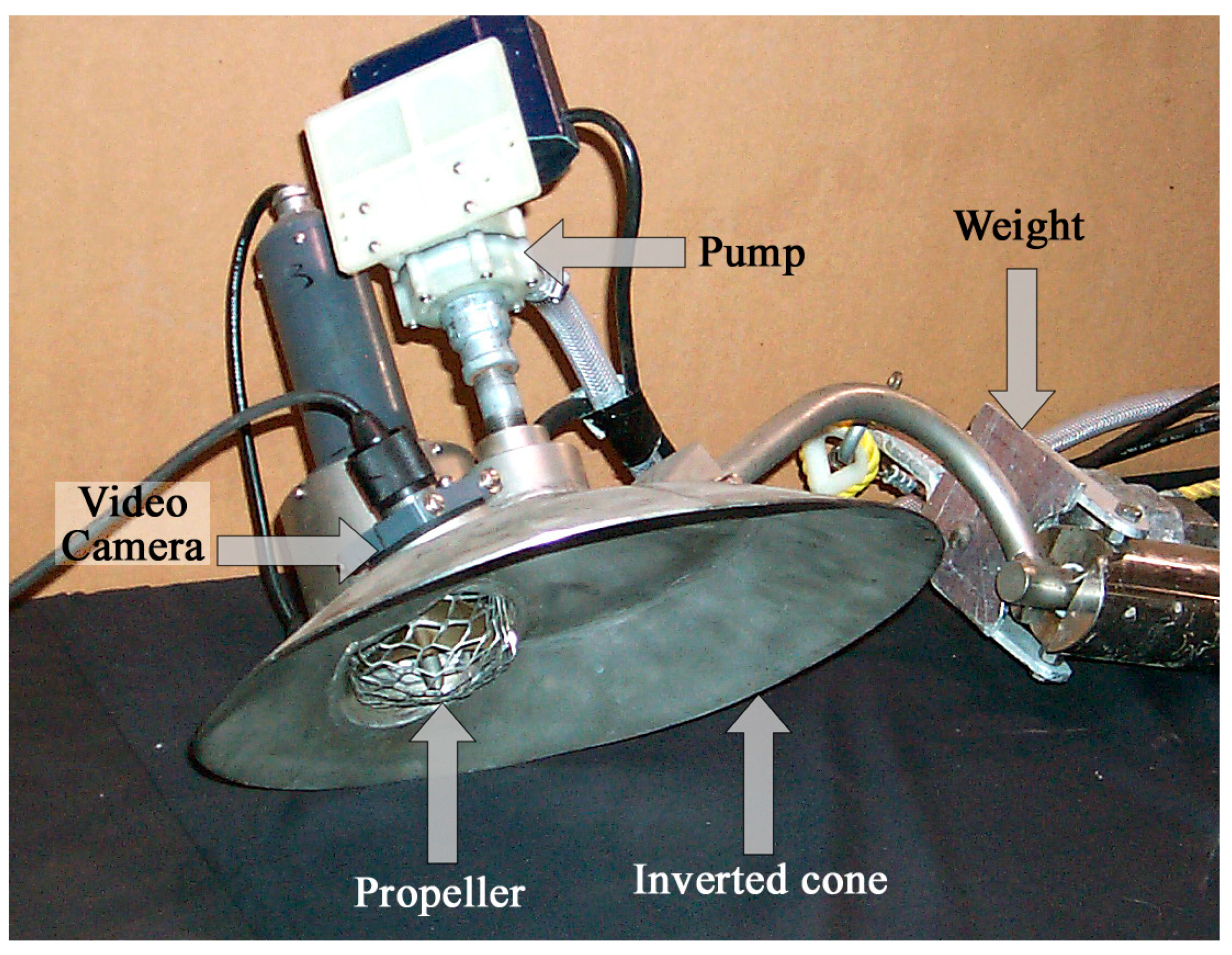
Figure 8.
Depositional characteristics of the Hay River sediment from the North-West Territories in Canada.
Figure 8.
Depositional characteristics of the Hay River sediment from the North-West Territories in Canada.
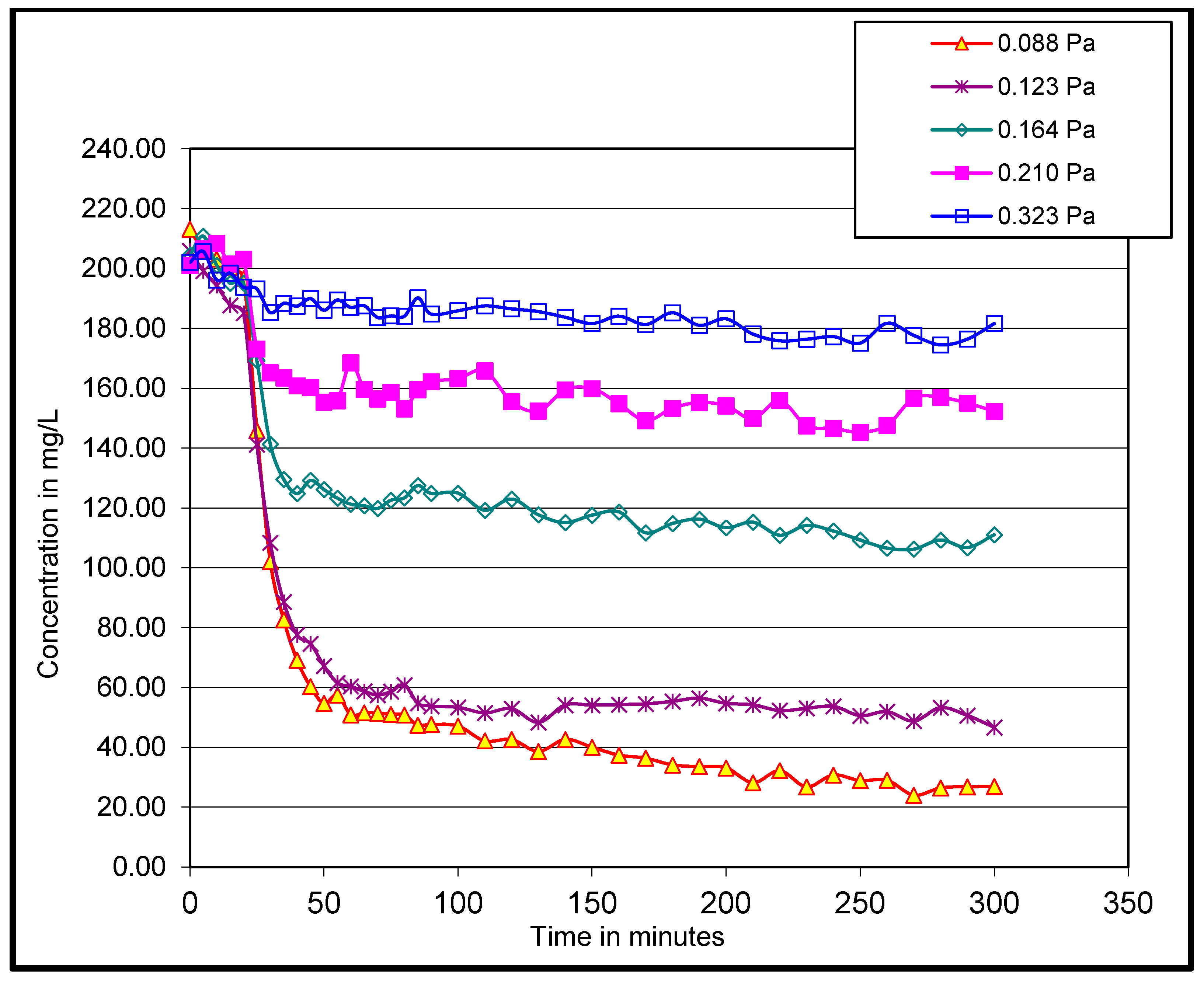
Figure 9.
Results from the erosion experiments for the Hay River sediment.
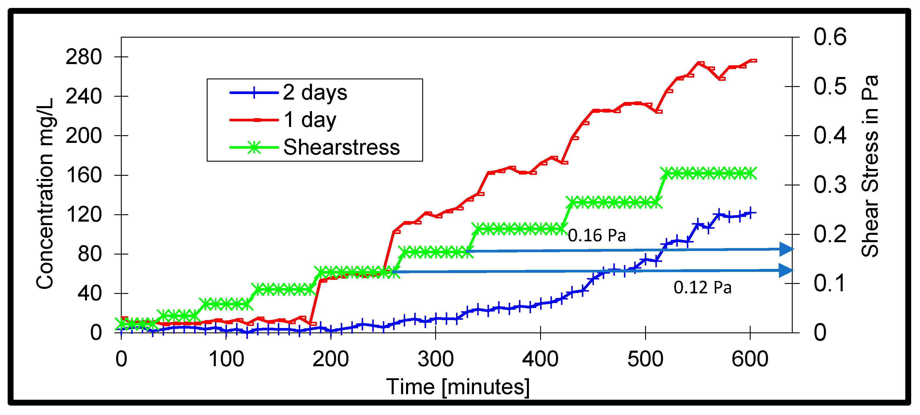
Figure 10.
Influence of initial concentration on the deposition process.

Figure 11.
Normalized concentration during deposition.
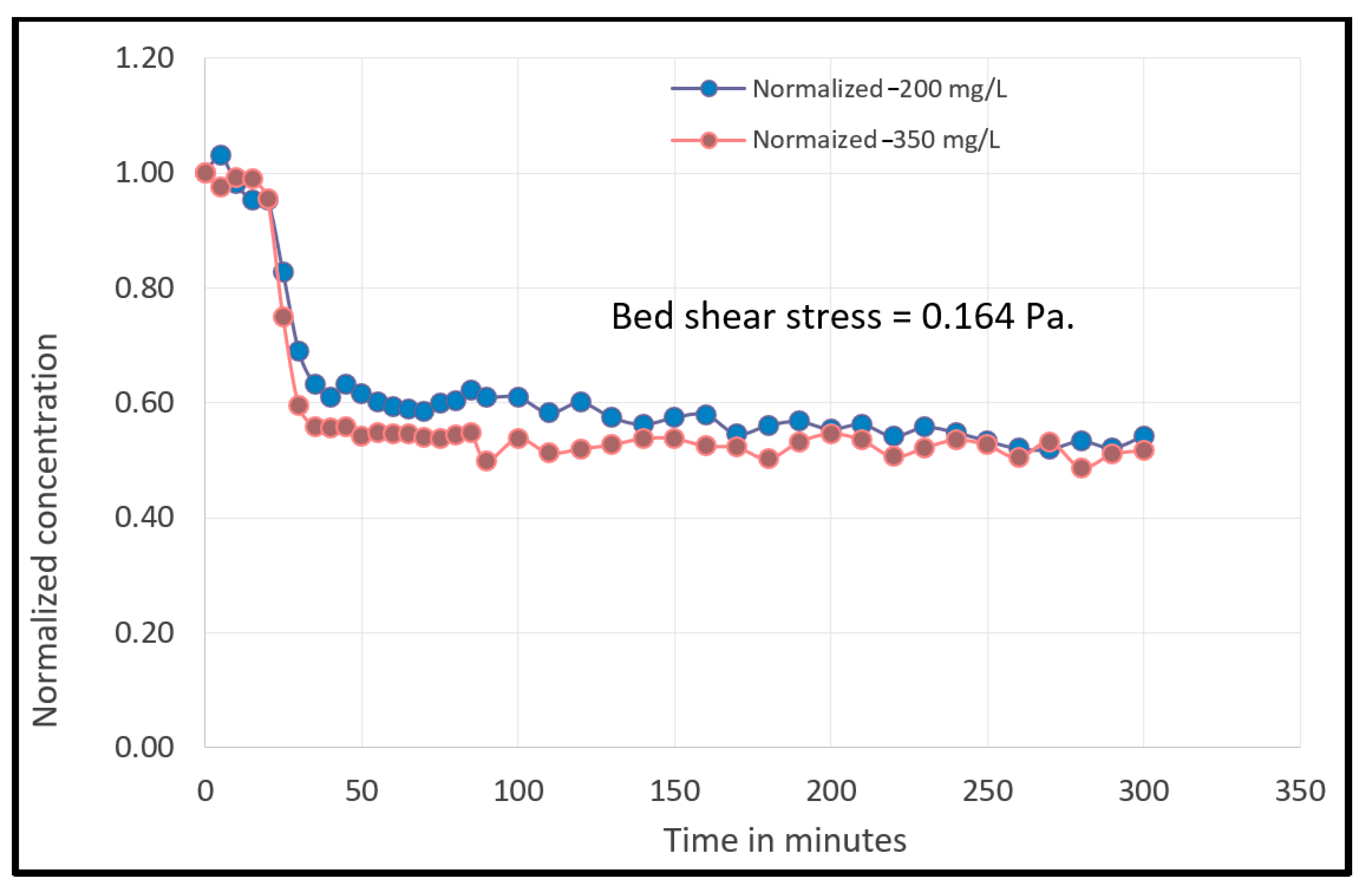
Figure 12.
Median size of flocs as a function of bed shear stress.

Figure 13.
Complete distribution of floc sizes: (A) bed shear stress of 0.088 Pa; (B) bed shear stress of 0.210 Pa; (C) bed shear stress of 0.323 Pa.
Figure 13.
Complete distribution of floc sizes: (A) bed shear stress of 0.088 Pa; (B) bed shear stress of 0.210 Pa; (C) bed shear stress of 0.323 Pa.
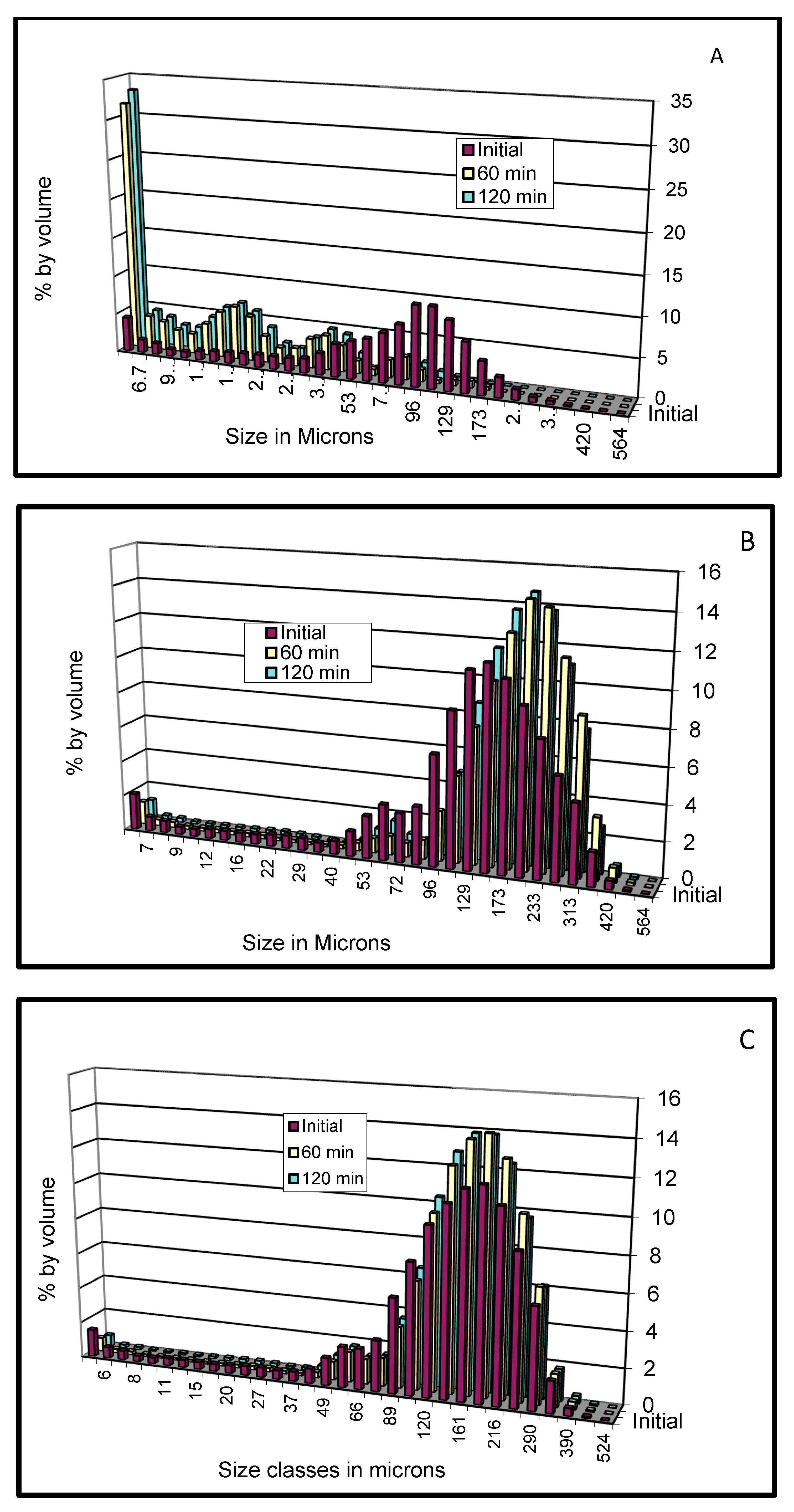
Figure 14.
Comparison between model predictions and measured deposition data.

Figure 15.
Comparison of measured and predicted size distribution during deposition under the shear stress of 0.323 Pa: (A) elapsed time of 30 min; (B) elapsed time of 60 min; (C) elapsed time of 120 min.
Figure 15.
Comparison of measured and predicted size distribution during deposition under the shear stress of 0.323 Pa: (A) elapsed time of 30 min; (B) elapsed time of 60 min; (C) elapsed time of 120 min.

Figure 16.
Density and settling velocity of sediment flocs from the Hay River.

Figure 17.
Variability of model parameters among different river systems: (A) critical shear stresses for erosion and deposition; (B) cohesion parameter; (C) empirical constants.
Figure 17.
Variability of model parameters among different river systems: (A) critical shear stresses for erosion and deposition; (B) cohesion parameter; (C) empirical constants.

Figure 18.
Settling velocity vs. floc size for the different river systems.
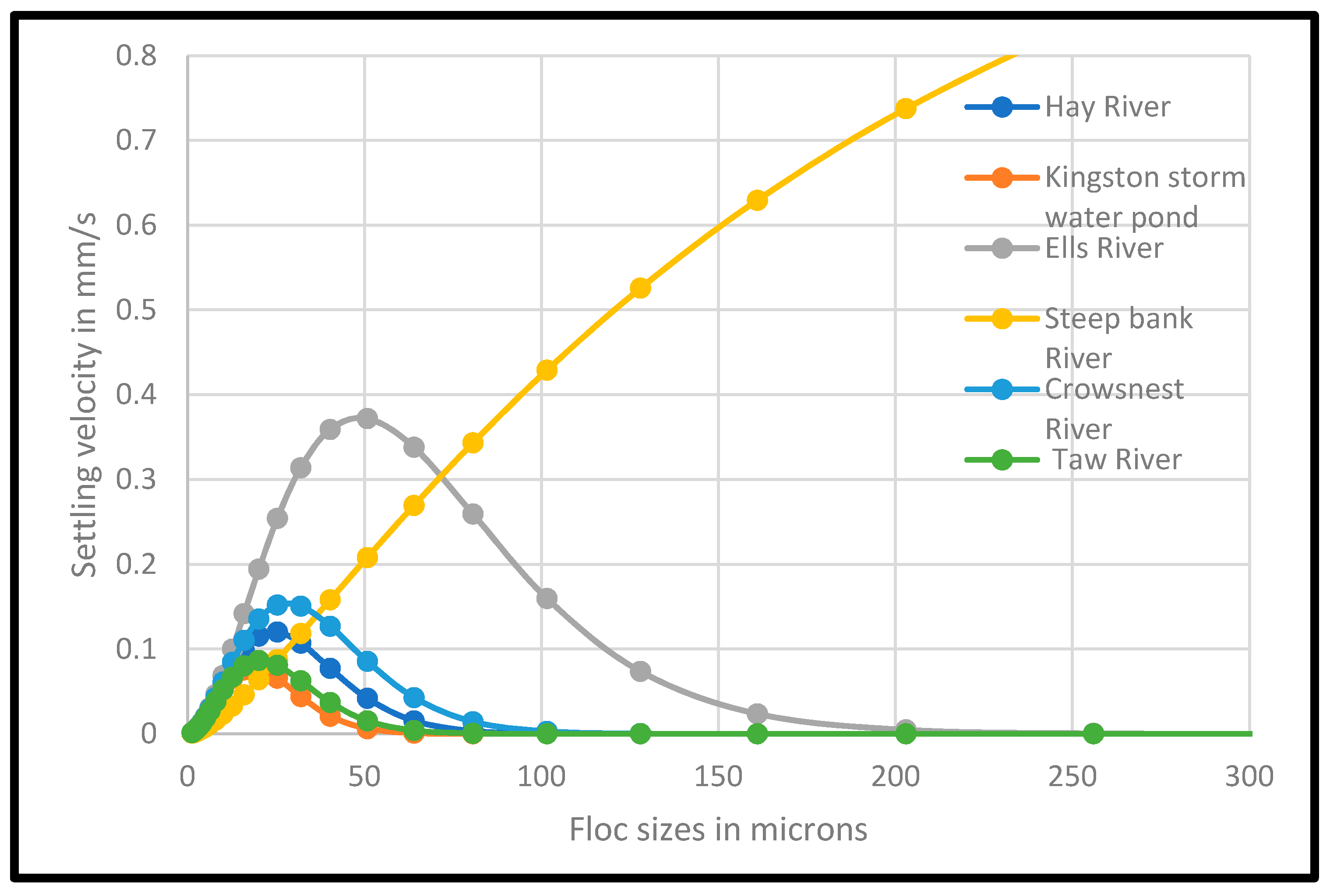
Figure 19.
Summary of entrapment experiments in the rotating circular flume.


Table 1.
Input data requirement for the RIVFLOC model.
| Number | Input Data Needed for RIVFLOC Model | Possible Sources of Such Data |
|---|---|---|
| 1 | The plan form of river- reach to supply the metric coefficient Mx | A field survey to measure the cross sections at a number of locations along the river reach. |
| 2 | Flow characteristics such as h, U and Q | A field measurement of h, U and Q or use the computational method described in Section 2.2. |
| 3 | Upstream boundary condition for sediment concentration | A field measurement at the upstream boundary of the model domain. |
| 4 | Upstream boundary condition for the size distribution of the sediment | A field measurement of size distribution of suspended sediment using instruments such as LISST (see Stone et al. [38]). |
| 5 | Transverse dispersion coefficient Ez | Literature data on transverse mixing in rivers. |
| 6 | Critical shear stress for erosion and deposition | Laboratory measurements using a rotating circular flume described in Section 2.3. |
| 7 | Cohesion parameter, β | Laboratory measurements using a rotating circular flume described in Section 2.3. |
| 8 | Empirical parameters b and c appearing in the relationship floc size vs. floc density | Laboratory measurement using a rotating circular flume described in Section 2.3. |
Table 2.
Listing of studies that employed the semi-empirical cohesive sediment transport model, RIVFLOC.
Table 2.
Listing of studies that employed the semi-empirical cohesive sediment transport model, RIVFLOC.
| River Systems | τcre Pa | τcrdp Pa | τcrdk Pa | β | Empirical Constants | References | |
|---|---|---|---|---|---|---|---|
| b 1 | c 1 | ||||||
| Hay River in NWT, Canada | 0.14 | 0.08 | 0.40 | 0.010 | 0.02 | 1.35 | Krishnappan [34] |
| Kingston, storm water pond, Canada | 0.10 | 0.05 | 0.50 | 0.075 | 0.02 | 1.45 | Krishnappan and Marsalek [35] |
| Ells River in Alberta, Canada | 0.01 | 0.004 | 0.25 | 0.006–0.03 | 0.02 | 1.15 | Droppo and Krishnappan [36] |
| Steepbank River in Alberta, Canada | 0.13 | 0.000 | 0.30 | 0.000 | 0.61 | 0.35 | Krishnappan [37] |
| Crowsnest River in Alberta, Canada | 0.18 | 0.09 | 0.50 | 0.075 | 0.02 | 1.30 | Stone et al. [38] |
| Taw River in UK | 0.09 | 0.06 | 0.40 | 0.13–0.25 | 0.02–0.025 | 1.15–1.35 | Stone et al. [39] |
1 Empirical constants appearing in Equation (10).
Table 3.
Maximum settling velocity and optimum floc size for different river systems.
| River Systems | Optimum Floc Size in Microns | Maximum Settling Velocity in mm/s |
|---|---|---|
| Kingston storm water pond, Canada | 20.0 | 0.08 |
| Taw River, UK | 20.0 | 0.09 |
| Hay River in NWT, Canada | 25.0 | 0.12 |
| Crowsnest River in Canada | 32.0 | 0.15 |
| Ells River in Canada | 51.0 | 0.37 |
| Steepbank River in Canada | n/a | Monotonic increase as a function of floc size |
Publisher’s Note: MDPI stays neutral with regard to jurisdictional claims in published maps and institutional affiliations. |
© 2022 by the author. Licensee MDPI, Basel, Switzerland. This article is an open access article distributed under the terms and conditions of the Creative Commons Attribution (CC BY) license (https://creativecommons.org/licenses/by/4.0/).
Share and Cite
MDPI and ACS Style
Krishnappan, B.G. Review of a Semi-Empirical Modelling Approach for Cohesive Sediment Transport in River Systems. Water 2022, 14, 256. https://doi.org/10.3390/w14020256
AMA Style
Krishnappan BG. Review of a Semi-Empirical Modelling Approach for Cohesive Sediment Transport in River Systems. Water. 2022; 14(2):256. https://doi.org/10.3390/w14020256
Chicago/Turabian StyleKrishnappan, Bommanna G. 2022. "Review of a Semi-Empirical Modelling Approach for Cohesive Sediment Transport in River Systems" Water 14, no. 2: 256. https://doi.org/10.3390/w14020256
Note that from the first issue of 2016, this journal uses article numbers instead of page numbers. See further details here.