
Ice Velocity in Upstream of Heilongjiang Based on UAV Low-Altitude Remote Sensing and the SIFT Algorithm


1
School of Water Conservancy and Civil Engineering, Northeast Agricultural University, Harbin 150030, China
2
Heilongjiang Provincial Key Laboratory of Water Resources and Water Conservancy Engineering in Cold Region, Harbin 150030, China
*
Author to whom correspondence should be addressed.
Water 2022, 14(12), 1957; https://doi.org/10.3390/w14121957
Submission received: 4 May 2022
/
Revised: 14 June 2022
/
Accepted: 16 June 2022
/
Published: 18 June 2022
(This article belongs to the Special Issue Sea, River, Lake Ice Properties and Their Applications in Practices)
Abstract
:In river management, it is important to obtain ice velocity quickly and accurately during ice flood periods. However, traditional ice velocity monitoring methods require buoys, which are costly and inefficient to distribute. It was found that UAV remote sensing images combined with machine vision technology yielded obvious practical advantages in ice velocity monitoring. Current research has mainly monitored sea ice velocity through GPS or satellite remote sensing technology, with few reports available on river ice velocity monitoring. Moreover, traditional river ice velocity monitoring methods are subjective. To solve the problems of existing time-consuming and inaccurate ice velocity monitoring methods, a new ice velocity extraction method based on UAV remote sensing technology is proposed in this article. In this study, the Mohe River section in Heilongjiang Province was chosen as the research area. High-resolution orthoimages were obtained with a UAV during the ice flood period, and feature points in drift ice images were then extracted with the scale-invariant feature transform (SIFT) algorithm. Moreover, the extracted feature points were matched with the brute force (BF) algorithm. According to optimization results obtained with the random sample consensus (RANSAC) algorithm, the motion trajectories of these feature points were tracked, and an ice displacement rate field was finally established. The results indicated that the average ice velocities in the research area reached 2.00 and 0.74 m/s, and the maximum ice velocities on the right side of the river center were 2.65 and 1.04 m/s at 16:00 on 25 April 2021 and 8:00 on 26 April 2021, respectively. The ice velocity decreased from the river center toward the river banks. The proposed ice velocity monitoring technique and reported data in this study could provide an effective reference for the prediction of ice flood disasters.
1. Introduction
Rivers north of 30° N in China generally develop ice hazards at the stages of winter river closure and spring river opening [1]. With increasing ice concentration and ice velocity in a given river section, the impact on hydraulic structures in the river increases. Upon river thawing in spring, specific river sections can become blocked by large amounts of ice, such as narrow river courses, shoals, sharp and continuous bends, and the front edges of unfrozen ice sheets. Ice accumulates to form ice jams or ice dams, which often severely block water flow sections and notably raise upstream water levels, resulting in ice jam flooding. Under long-term severe ice conditions, the impact of ice drift in spring can cause varying degrees of damage to hydraulic structures such as piers and bank revetments, threaten the lives and property of people, and further increase the difficulty of ice flood prevention [2]. Therefore, feasible and accurate ice velocity monitoring technology constitutes a major problem urgently requiring a solution in the field of water disasters. Ice velocity monitoring is not only the main priority in the fields of major natural disaster monitoring and mitigation, but is also one of the major problems related to water engineering safety, the national economy, livelihoods of people, and social development [3].
At present, some achievements had been made regarding the velocity measurements of sea ice and glaciers. Sea ice velocity monitoring methods are mainly divided into two categories: field observation methods and remote sensing monitoring methods [4]. Of these categories, field observation methods mainly include marker monitoring methods and global positioning system (GPS)-based monitoring methods [5,6], whereas remote sensing monitoring methods are largely categorized into optical and microwave remote sensing monitoring methods [7,8]. The methods applied in river ice velocity monitoring are mostly field observation methods [9], for example, visual tracking methods [10]. These methods rely on a simple principle but require highly experienced observers. Moreover, field observation methods exhibit notable subjectivity and high time and labor costs, and these methods are unsuitable for large-scale and long-term tracking. In the GPS monitoring method [11], large ice blocks with a good shape are selected, GPS sensors are installed atop these ice blocks, and the instantaneous speed of the ice blocks equipped with GPS sensors is monitored in real time with a high accuracy through the positioning mode involving a satellite, GPS sensors, and base station. For example, Song Chunshan et al. [12] measured the ice drift velocity in the upper reaches of the Heilongjiang River with the GPS monitoring method in 2019 and studied the drift ice blocking phenomenon in each reach during the ice flood period based on the velocity variation. However, the GPS tracking method can only obtain the velocity of a single ice block but cannot obtain the ice velocity field in large-scale areas, and the observation process (sensor placement and recovery) results in a high time cost and difficulty. Deng Xiao et al. [13] set up a camera on the shore, manually selected two images at a certain time interval in the obtained monitoring footage, and determined the moving distance of drift ice to calculate the ice drift velocity. However, due to the influence of side view, images typically suffer the problem of image geometric distortion, which affects the monitoring accuracy. In addition, it takes a long time to process data manually.
With the continuous improvement of unmanned aerial vehicles (UAVs) and sensor technology, small UAVs have been widely deployed in low-altitude remote sensing measurements [14,15,16,17]. Compared to the visual and GPS-based tracking methods, the multisensor UAV platform exhibits the characteristics of high efficiency, low cost, flexible operation, and strong suitability in complex river environments. This technique not only overcomes the difficulty of image data acquisition but also avoids the image distortion phenomenon attributed to side shooting from the shore, which improves the accuracy of the original data and provides a new technical means for ice velocity monitoring within a large range.
To solve the above problems, this paper proposes the combination of the SIFT and RANSAC algorithms to track feature points and researches the velocity vector of drift ice on this basis. To verify the feasibility of the proposed method, the Mohe section located in the upper reaches of Heilongjiang Province is selected as the observation area. An UAV is employed to obtain high-resolution video data during the ice flood period. Images are processed in OpenCV software that are automatically extracted at 1-s intervals in video. Subsequently, the ice plane velocity field in the observation area is extracted to perform ice dynamic analysis, thus providing a suitable technique and reference data for ice flood disaster early warnings and prediction.
2. Materials and Methods
2.1. Overview of the Research Area
The Heilongjiang River is located in the northernmost part of China, with a wide drainage area and abundant water resources. The drainage basin is located in the cold temperate zone. The ice thickness can reach 2 m in winter, and the ice surface is covered with snow exhibiting an average thickness of 30 cm [18]. Due to the unique geographical location of Heilongjiang, the upper reaches of the Heilongjiang River flow from low latitudes to high latitudes [19] through mountainous areas with narrow and tortuous river courses. There is abundant rainfall and runoff but insufficient observation equipment and measurement means. During the ice flood period, ice mainly accumulates in the Mohe section to form ice dams [20]. Therefore, the research area is the Mohe section in Heilongjiang Province, and the takeoff and landing point of the UAV is an open area southeast of the Mohe hydrological station (as shown in Figure 1).
2.2. Research Method
At 16:00 on 25 April 2021 and 8:00 on 26 April 2021, a DJI quad-rotor small UAV (Mavic 2 Pro) was employed for fixed-point shooting. The UAV is equipped with a Hasselblad L1d-20c (CMOS) aerial camera with an effective resolution of 20 million pixels and can record 4K high-dynamic range (HDR) footage. The weather conditions captured in each aerial photograph were sunny, the wind speed was lower than 10.7 m/s, the flight altitude was set to 400 m, the elevation difference between the take-off point and water surface was 5 m, the lens was oriented vertically downward, and the UAV hovered during shooting.
In this study, the tracking process of ice feature points included four main steps. Step 1. Feature point selection. First, a large number of ice feature points were extracted from the phase I image (a certain frame of image in the observation video) with the SIFT operator, and ice feature points were extracted from the phase II image (the frame of image after 1 s in the observation video) in the same way.
Step 2. Feature point matching. Based on the Euclidean distance, a BF matcher was adopted to track the same feature points in the above two images.
Step 3. Match result filtering. The obtained matching feature point pairs were filtered with the RANSAC algorithm to remove any incorrect matching feature point pairs.
Step 4. Ice velocity determination. The relationship between the UAV height and the actual length represented by a unit pixel was determined through calibration, the distance of the filtered feature point pairs was transformed into the moving distance of drift ice, and, finally, the ice drift velocity was determined.
2.2.1. Feature Point Selection
The SIFT algorithm is a feature point detection algorithm based on the scale space first proposed by Lowe [21] in 1999 and formally put forward after summary and improvement in 2004 [22]. A difference of Gaussian (DOG) scale space is constructed. The scale space describes the original image at different levels, and the different levels are represented by various scale parameters. Koenderink [23] and Lindeberg [24] demonstrated that the Gaussian kernel is the only linear kernel for scale space construction.
The Gaussian function of scale transformation is defined as:
Image scale space function L(x, y, σ) is expressed as:
where I(x, y) is the input image, G(x, y, σ) is a variable-scale Gaussian operator, ⊗ is the convolution operation, and σ is the mean square deviation of the Gaussian normal distribution, which is denoted as the spatial scale factor. The larger the σ value, the more blurred the image becomes. Conversely, the smaller the σ value, the clearer the image becomes. To ensure that the extreme points in the scale space attain a suitable uniqueness and stability, Lowe [22] proposed the DOG concept, which is the difference between two adjacent scale images.
The calculation equation of the differential Gaussian image is as follows:
where k is a constant factor of the difference between adjacent scale images, and the k value is related to the number of pictures (S) in each layer of the scale space, i.e., .
After construction of the DOG pyramid, it is necessary to select key points from the pyramid scale space, namely, local feature extreme points in the image space. Each sampling point is compared to 8 adjacent points in the current scale layer and 18 points in the upper and lower adjacent scale layers to determine whether the considered sampling point is an extreme point in the current scale space and two-dimensional space [25].
Because the extreme points detected with the above method are distributed in the discrete space, the extreme points in the known discrete space are interpolated to extreme points in the continuous space through subpixel interpolation. To obtain the exact position of an extreme point, the DOG function is expanded according to the Taylor formula as follows:
where D is the D(x, y, σ) value at the feature point position and X = (x, y, σ)T is the offset relative to this feature point. The extreme value of D(x) is determined, i.e., , and the position of the extreme point is:
The extreme value at the corresponding extreme point is:
If , this feature point is removed as an unstable feature point. Because the DOG operator can produce strong edge responses, it is necessary to apply the Hessian matrix at the feature points to eliminate points with an unstable edge response [26]. The Hessian matrix is defined as:
where Dxx, Dxy, and Dyy denote derivations of x or y.
Among the accurately located stable feature points, the parameter direction is specified for each feature point based on the gradient direction distribution characteristics of its neighborhood pixels, and the feature vector is then generated relative to this direction so that the SIFT-determined feature points remain invariant to image rotation.
Gradient modulus:
Gradient direction:
Through the above process, the feature points contain three basic components of information: position, scale, and direction. Moreover, the feature points are invariant to translation, scaling, and rotation. To ensure that the feature points remain unchanged under various conditions, such as solar radiation level and viewing angle, a descriptor is established for each feature point. The feature point is adopted as the center, the coordinate axis of the image is rotated to match the direction along which the feature point is located, the neighborhood near the feature point is divided into 4 × 4 subwindows, the gradient information in each subwindow is obtained, an 8-dimensional direction histogram is generated, a 128-dimensional feature descriptor is finally established, and the descriptor subvector elements are normalized to improve the resistance to light changes [27].
2.2.2. Feature Point Matching
The BF matcher is a simple matching algorithm. Suppose the set of all feature points in image P1 is {a1, a2, …an}, and the set of all feature points in image P2 is expressed as {b1, b2, …bn}. When the BF matcher is applied to match the feature points in images P1 and P2, the Euclidean distance from the feature vectors of each feature point in image P1 to each feature point in image P2 is calculated. The result of the algorithm is an n × m-dimensional matrix , where dij is the Euclidean distance between the feature vectors of feature points ai and bj [28].
2.2.3. Match Result Filtering
After all feature points are matched, incorrect matching points inevitably occur, which can affect the accuracy of ice velocity calculation. In this paper, the RANSAC algorithm is implemented to further optimize the matching results, and the matching feature points are screened through continuous iteration.
The RANSAC algorithm is an iterative algorithm proposed by Fischler and Bolles [29] to estimate the parameters of mathematical models. This algorithm has been widely applied in line fitting and plane fitting. Correct data contained in the considered data are recorded as inner points, and abnormal data (or noise) are recorded as outer points [30]. The probability of obtaining the correct model through the RANSAC algorithm is:
where P is the probability of the inner points, K is the minimum number of data points required to solve the model, and M is the number of iterations. The above equation yields the following:
Finally, optimal matching feature point pairs are obtained, i.e., the feature point pairs with the same name between the input phase I ice image and matching phase II ice image.
2.2.4. Ice Velocity Calculation
After all feature point pairs with the same feature descriptor are obtained, the horizontal displacement of ice can be extracted, and the feature point pairs with the same feature descriptor can then be transformed into the ice velocity according to the pixel scale and image interval, as follows:
where X1, X2, Y1, and Y2 are the coordinates of the feature point pairs with the same feature descriptor, S is the moving distance of the feature point in the image (px), R is the pixel scale (cm/px), T is the time between the two images (s), and V is the ice velocity (m/s).
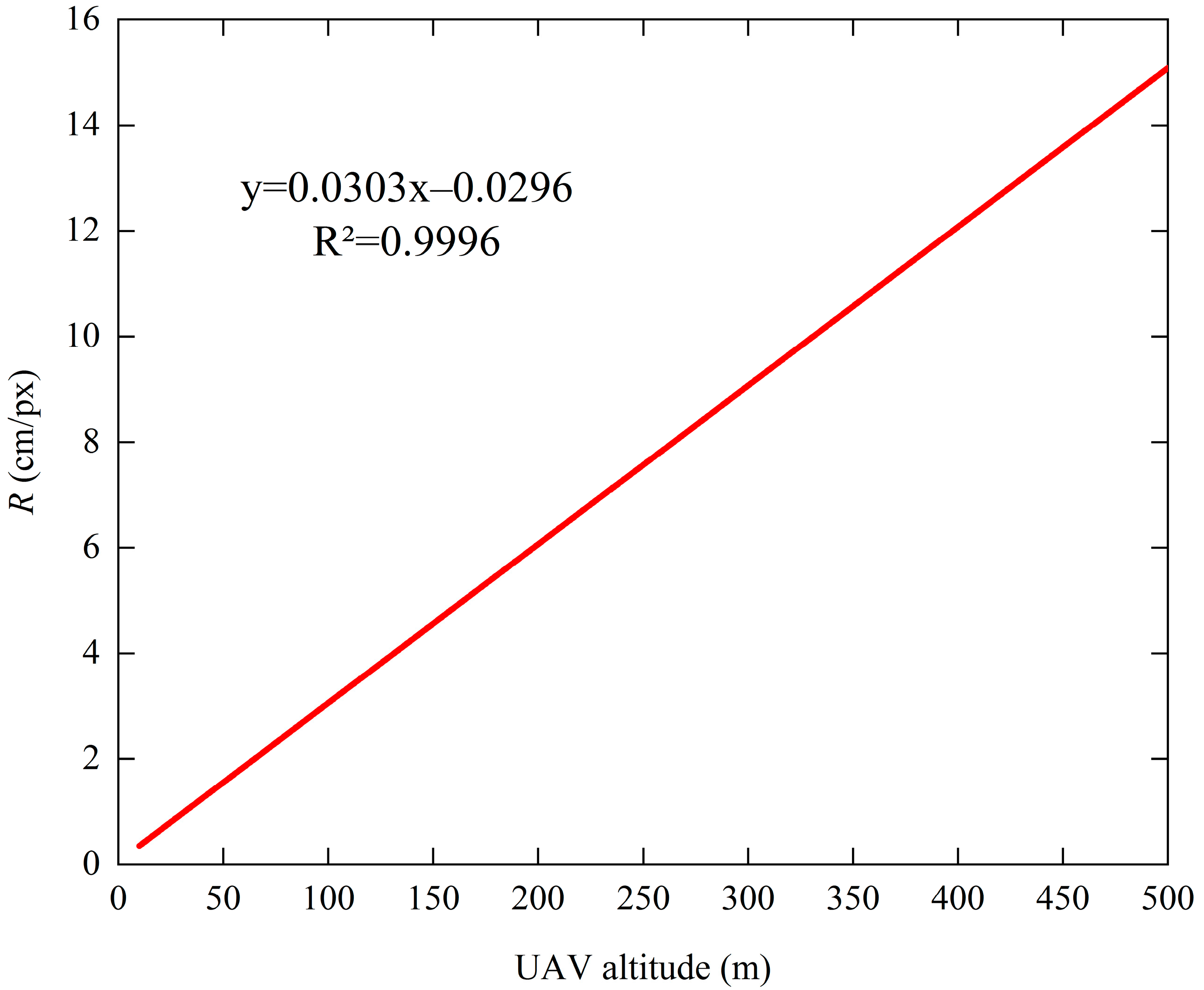
To realize quantitative analysis of the ice velocity, first, the UAV is deployed to shoot A1-sized paper panels at different heights to determine the shooting height of UAV remote sensing images and the actual area represented by a unit pixel. After the actual area is squared, a fitting equation between the unit pixel length and actual length in remote sensing images at the different heights is obtained, as shown in Figure 2.
3. Results
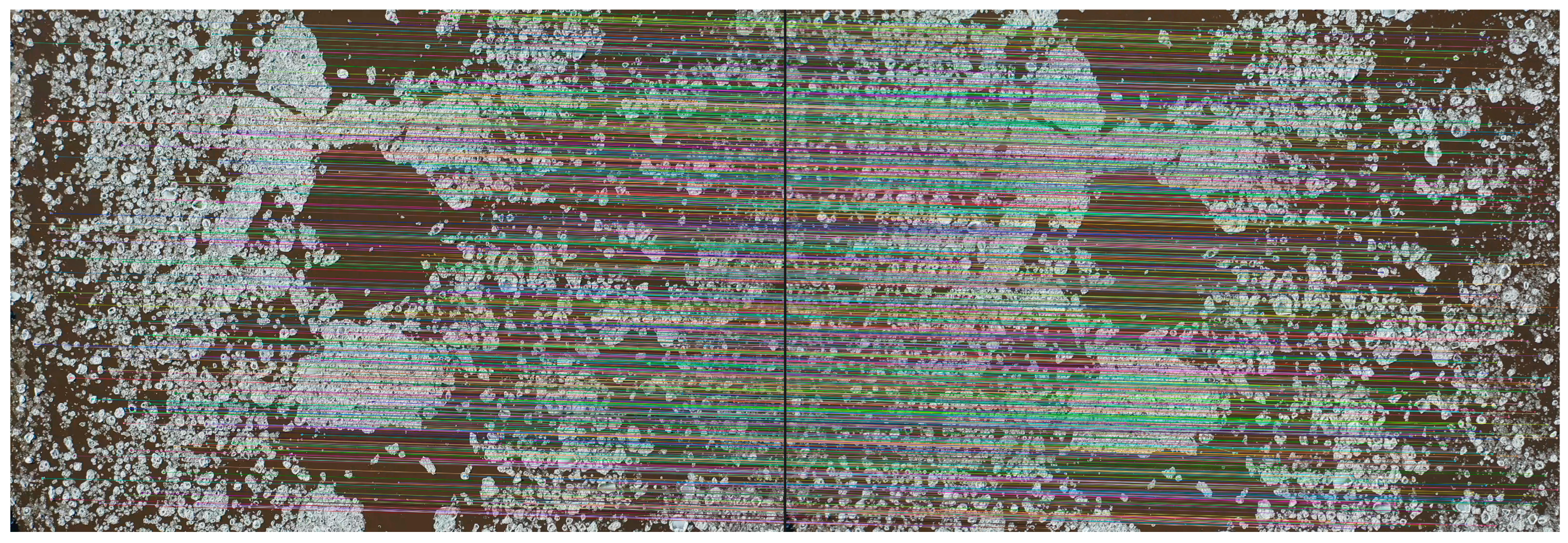
Through feature point selection, matching, and filtration of the two obtained orthophoto images, 1429 pairs of effective feature points (as shown in Figure 3) were extracted from the river section at 16:00 on 25 April 2021, and 2726 pairs of effective feature points (as shown in Figure 4) were extracted from the river section at 8:00 on 26 April 2021. According to the principle of feature point selection, there were sparse or even absent feature extreme points on the river surface, but the distribution of the feature points on the ice surface was relatively dense and stable, which satisfied the basic requirements of ice velocity analysis. At 8:00 on 26 April 2021, due to the large amount of broken ice in the river section, the selected effective feature point density was higher than that at 16:00 on 25 April 2021.
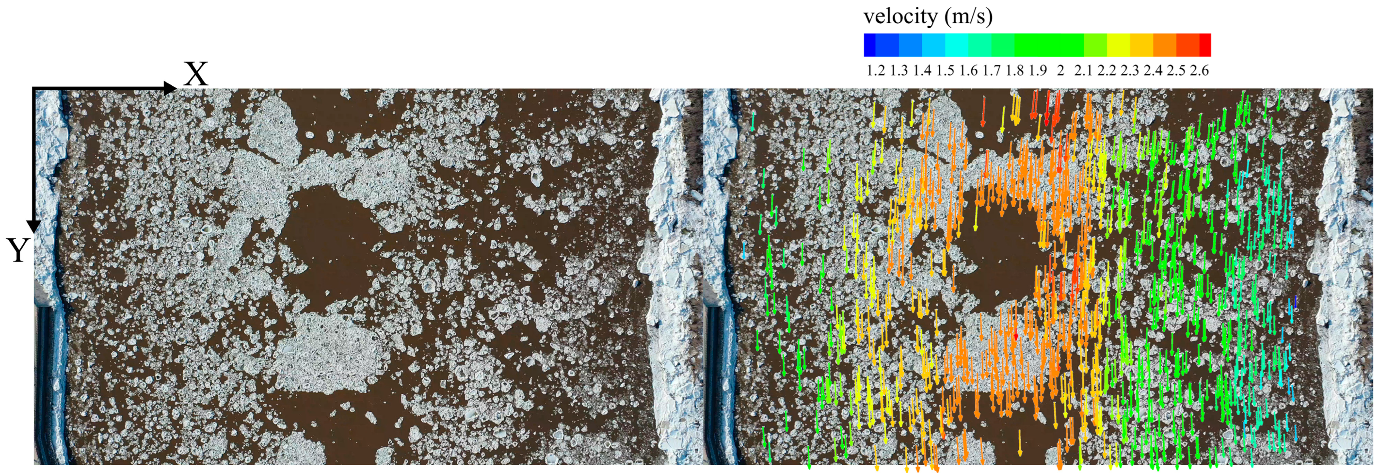
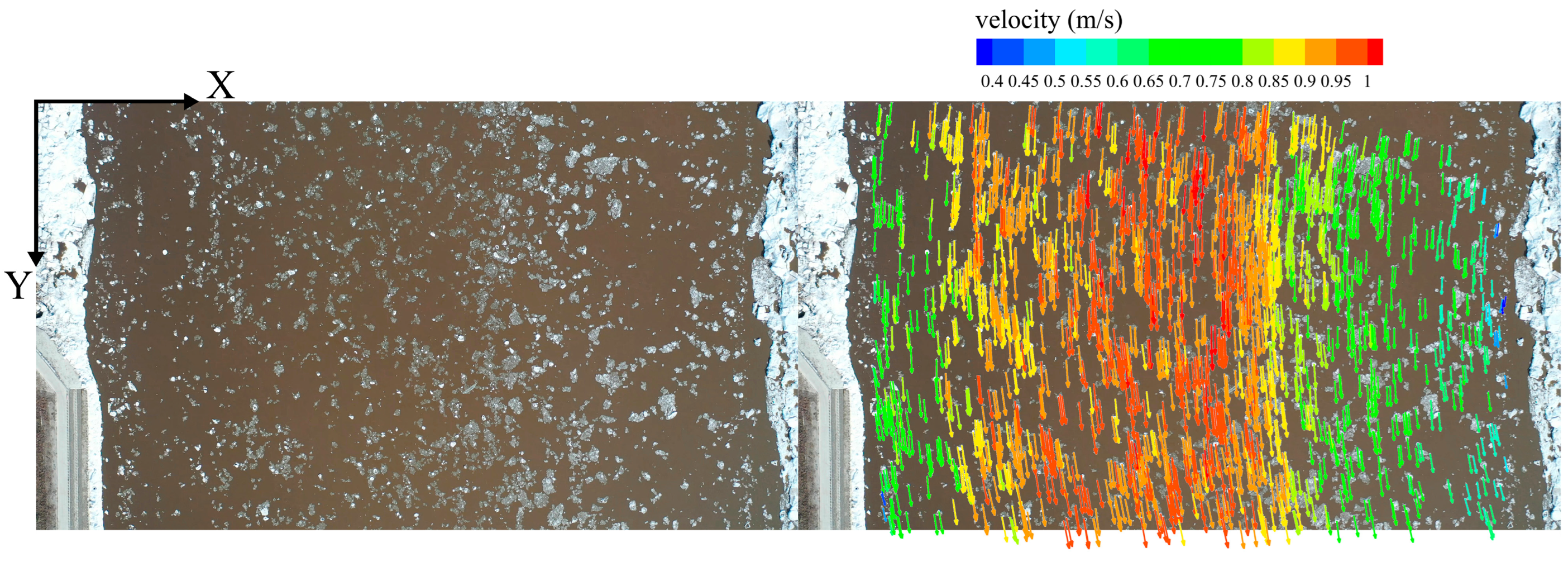
The ice velocity in the Mohe section in Heilongjiang at 16:00 on 25 April and at 8:00 on 26 April 2021 was extracted, as shown in Figure 5 and Figure 6, respectively. The distribution characteristics of the ice velocity are similar. Affected by the river bend, areas with the highest ice velocity were concentrated on the right side of the river center, and the ice velocity tended to decrease toward the banks on both sides. Moreover, there occurred a sudden change in the ice flow velocity near the river banks on both sides, which was likely caused by collision between drift ice and the bank slopes. Figure 7a,b show a statistical histogram of the ice velocity at 16:00 on 25 April and 8:00 on 26 April 2021. The figure shows that at 16:00 on 25 April 2021, the ice velocity was mostly in the range 2.40~2.50 m/s, accounting for 30.02% of all velocity values. The maximum, minimum, and average ice velocities were2.65 m/s, 1.11 m/s, and 2.00 m/s, respectively. At 8:00 on 26 April 2021, the ice velocity was largely in the range 0.90~1.00 m/s, accounting for 50.33% of all velocity values. The maximum, minimum, and average ice velocities were 1.04 m/s, 0.38 m/s, and 0.74 m/s, respectively. Compared to 16:00 on 25 April 2021, the standard deviation of the ice velocity at 8:00 on 26 April 2021 was 0.18, and the ice velocity distribution was more uniform.
4. Discussion
4.1. Ice Velocity Analysis
At 18:35 on 24 April 2021, the upstream ice dam burst, and the water level in the study area encompassing the Mohe section changed sharply. From 18:35 on 24 April 2021 to 5:00 on 25 April 2021, ice jams were formed many times downstream of the Mohe section research area, resulting in rapid water level rise in the research area. Until 5:00 on 25 April 2021, the Mohe section in Heilongjiang remained fully open, the water level in the research area decreased rapidly, and the ice velocity was high. At 16:00 on 25 April, the average velocity of ice was 2.00 m/s. At 8:00 on 26 April 2021, the water level in the research area dropped to the normal level, the ice flood period in Heilongjiang had basically ended (as shown in Figure 8), the ice velocity was low, and the average velocity of ice reached 0.74 m/s, which was in line with the actual situation.
To study the distribution characteristics of the ice velocity during the ice flood period in the Mohe section of Heilongjiang more comprehensively, the transverse and longitudinal components of the ice velocity during the different periods were calculated by tracking the displacement components of the effective characteristic points in the corresponding coordinate system. For this calculation, Vx is the transverse component of ice velocity, Vy is the longitudinal component of ice velocity, and the positive and negative symbols indicate the direction of the velocity component. According to the schematic diagram of the observation geographical location, the observation area is located at a river bend. As indicated by the transverse velocity component shown in Figure 9a,c, the ice velocity upstream of the river was biased to the right side of the river, which can easily damage the right bank of the river, form ice accumulation, seriously block the water crossing section, and threaten the lives and property of people. For example, the ice accumulation and damage to the bank slope are shown in Figure 10, which are in line with the actual site conditions. As indicated by the longitudinal velocity component depicted in Figure 9b,d, the ice velocity was oriented along the river channel, and there occurred no ice reflux phenomenon affected by vortexing.
To highlight the significance of this research, the related research results are compared. Deng Xiao [13] carried out a series of studies on the ice velocity in the Heilongjiang River. Under the assumption that the ice flows horizontally, the ice velocity was confirmed by manual processing. It needs to be noted that the average velocity of ice was 1.62 m/s and the image data were recorded at 10:28 on 2 May 2016. The ice movement at different times are shown in Figure 11. Although the ice velocity can be determined, this method can only manually acquire the velocity for a single ice block, and this method typically suffers the problem of image geometric distortion, which affects the monitoring accuracy and is time consuming. In addition, Chave [31] installed a real time data acquisition system in Lake St. Pierre in the St. Lawrence River to measure the ice velocity. The system can work around the clock. Unfortunately, the instruments often work underwater and cannot be moved. Therefore, the cost of installation and maintenance is not economical. However, the proposed method, UAV combined with SIFT and RANSAC algorithms, can fill these gaps. The velocity of ice blocks can be determined simultaneously, and a large number of in situ monitoring instruments are not required. In addition, the proposed method is suitable for ice running at high speed.
4.2. Ice Velocity Verification
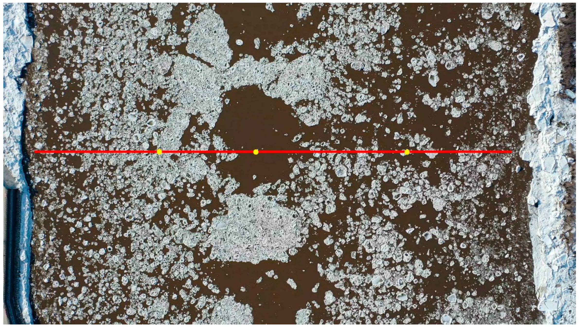
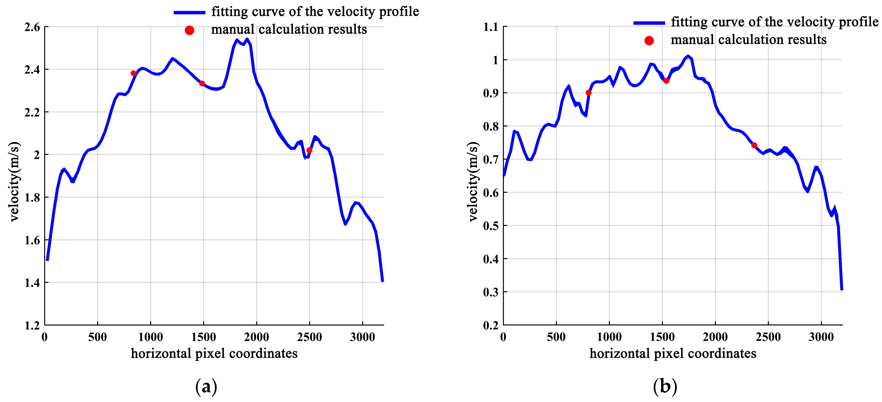
Upon completion of feature point matching in ice images obtained with the UAV, although the matching results are further screened with the RANSAC algorithm, ice may collide with other ice blocks or bank slopes, thus changing the local extreme points, which can lead to incorrect matching or the absence of feature point pairs in images. To quantitatively evaluate the accuracy of ice velocity determination in the research area, ice was selected in the river section, feature points with the same name were extracted through visual interpretation (as shown in Figure 12), the ice velocity was manually calculated, and the obtained calculation value was compared to the ice velocity within 1 m before and after the section based on the SIFT algorithm, as shown in Figure 13a,b, respectively. The errors were less than 0.02 m/s. It was determined that the ice velocity determined based on the SIFT algorithm was consistent with the actual situation.
5. Conclusions
To monitor and realize in-depth analysis of ice change information, this paper tracks ice surface feature points based on UAV remote sensing images and the SIFT algorithm, establishes the corresponding ice velocity field, and finally carries out in-depth analysis and interpretation of ice movement based on the established ice velocity field. The following conclusions are obtained:
- Feature points were selected as local extreme points. Only ice surfaces, edges, and corners can produce dense and stable feature points. The SIFT algorithm provided the advantages of high precision and notable robustness. The SIFT and RANSAC algorithms were jointly employed to track the feature points, which realized ice velocity monitoring.
- At 16:00 on 25 April 2021, the ice velocity was mostly in the range 2.40~2.50 m/s, accounting for 30.02% of all velocity values. The maximum, minimum, and average ice velocities were2.65 m/s, 1.11 m/s, and 2.00 m/s, respectively. At 8:00 on 26 April 2021, the ice velocity was mainly in the range 0.90~1.00 m/s, accounting for 50.33% of all velocity values. The maximum, minimum, and average ice velocities were1.04 m/s, 0.38 m/s, and 0.74 m/s, respectively. The areas with the highest ice velocity in the studied reach were concentrated on the right side of the river center, and the ice velocity tended to decrease toward the banks on both sides. In addition, based on the ice velocity field, ice accumulation formation on the bank slope was highly related to the ice velocity.
- Under the influence of illumination changes and ice collisions, the local extreme points varied. The matching results were further screened with the RANSAC algorithm. The error between the ice velocity obtained with the SIFT algorithm and the manually calculated ice velocity was less than 0.02 m/s, which was in line with the actual situation.
- Compared to traditional ice velocity monitoring methods, the proposed method attained a high precision, and greatly reduced time and labor costs. The research method in this paper provides a new technical means for large-scale ice change information monitoring. In the future, we can perform further research on ice jams and ice dams based on this technique.
Author Contributions
Conceptualization, E.W. and H.H.; methodology, E.W., S.H. and H.H.; formal analysis, S.H. and H.H.; investigation, E.W., S.H., Y.L., Z.R. and S.D.; data curation, S.H., Y.L., Z.R. and S.D.; writing—original draft preparation, E.W. and S.H.; writing—review and editing, H.H.; funding acquisition, E.W. All authors have read and agreed to the published version of the manuscript.
Funding
This research was supported by the National Natural Science Foundation of China (41876213), the National Key R&D Program of China (No.2018YFC0407301-03) and the Natural Science Foundation of Heilongjiang Province of China (No. LH2020E004).
Institutional Review Board Statement
Not applicable.
Informed Consent Statement
Not applicable.
Data Availability Statement
The data are available in the case that they are required.
Conflicts of Interest
The authors declare no conflict of interest.
References
- Goldberg, M.D.; Li, S.; Lindsey, D.T.; Sjoberg, W.; Zhou, L.; Sun, D. Mapping, Monitoring, and Prediction of Floods Due to Ice Jam and Snowmelt with Operational Weather Satellites. Remote Sens. 2020, 12, 1865. [Google Scholar] [CrossRef]
- Wang, J.; Shi, F.-y.; Chen, P.-p.; Wu, P.; Sui, J. Impact of bridge pier on the stability of ice jam. J. Hydrodyn. 2015, 27, 865–871. [Google Scholar] [CrossRef]
- Wang, R.; Huang, D.; Zhang, X.; Wei, P. Combined pattern matching and feature tracking for Bohai Sea ice drift detection using Gaofen-4 imagery. Int. J. Remote Sens. 2020, 41, 7486–7508. [Google Scholar] [CrossRef]
- Heid, T.; Kääb, A. Evaluation of existing image matching methods for deriving glacier surface displacements globally from optical satellite imagery. Remote Sens. Environ. 2012, 118, 339–355. [Google Scholar] [CrossRef]
- Dorrer, E.; Hofmann, W.; Seufert, W. Geodetic results of the Ross Ice Shelf Survey expeditions, 1962–1963 and 1965–66. J. Glaciol. 1969, 8, 67–90. [Google Scholar] [CrossRef]
- Manson, R.; Coleman, R.; Morgan, P.; King, M. Ice velocities of the Lambert Glacier from static GPS observations. Earth Planets Space 2000, 52, 1031–1036. [Google Scholar] [CrossRef] [Green Version]
- Chaouch, N.; Temimi, M.; Romanov, P.; Cabrera, R.; McKillop, G.; Khanbilvardi, R. An automated algorithm for river ice monitoring over the Susquehanna River using the MODIS data. Hydrol. Processes 2014, 28, 62–73. [Google Scholar] [CrossRef]
- Heygster, G.; Alexandrov, V.; Dybkjær, G.; Hoyningen-Huene, W.v.; Girard-Ardhuin, F.; Katsev, I.; Kokhanovsky, A.; Lavergne, T.; Malinka, A.; Melsheimer, C. Remote sensing of sea ice: Advances during the DAMOCLES project. Cryosphere 2012, 6, 1411–1434. [Google Scholar] [CrossRef] [Green Version]
- Shen, H.T.; Liu, L. Shokotsu River ice jam formation. Cold Reg. Sci. Technol. 2003, 37, 35–49. [Google Scholar] [CrossRef]
- Ozsoy-Cicek, B.; Kern, S.; Ackley, S.F.; Xie, H.; Tekeli, A.E. Intercomparisons of Antarctic sea ice types from visual ship, RADARSAT-1 SAR, Envisat ASAR, QuikSCAT, and AMSR-E satellite observations in the Bellingshausen Sea. Deep Sea Res. Part II 2011, 58, 1092–1111. [Google Scholar] [CrossRef]
- Gleason, S. Towards sea ice remote sensing with space detected GPS signals: Demonstration of technical feasibility and initial consistency check using low resolution sea ice information. Remote Sens. 2010, 2, 2017–2039. [Google Scholar] [CrossRef] [Green Version]
- Song, C.S.; Zhu, X.Y.; Han, H.W.; Lin, L.B.; Yao, Z. The influence of riverway characteristics on the generation and dissipation of ice dam in the upper reaches of Heilongjiang River. J. Hydrol. Eng. 2020, 51, 1256–1266. (In Chinese) [Google Scholar]
- Deng, X.; Wang, D.R.; Feng, J.; Zhang, L.; Qin, J.M. Image correction algorithm optimization and system design for ice density monitoring. J. Taiyuan Univ. Technol. 2020, 51, 310–315. (In Chinese) [Google Scholar]
- Bushaw, J.D.; Ringelman, K.M.; Johnson, M.K.; Rohrer, T.; Rohwer, F.C. Applications of an unmanned aerial vehicle and thermal-imaging camera to study ducks nesting over water. J. Field Ornithol. 2020, 91, 409–420. [Google Scholar] [CrossRef]
- Hunter III, J.E.; Gannon, T.W.; Richardson, R.J.; Yelverton, F.H.; Leon, R.G. Integration of remote-weed mapping and an autonomous spraying unmanned aerial vehicle for site-specific weed management. Pest Manag. Sci. 2020, 76, 1386–1392. [Google Scholar] [CrossRef] [PubMed] [Green Version]
- Shafer, M.W.; Vega, G.; Rothfus, K.; Flikkema, P. UAV wildlife radiotelemetry: System and methods of localization. Methods Ecol. Evol. 2019, 10, 1783–1795. [Google Scholar] [CrossRef]
- Kalke, H.; Loewen, M. Support vector machine learning applied to digital images of river ice conditions. Cold Reg. Sci. Technol. 2018, 155, 225–236. [Google Scholar] [CrossRef]
- Wang, H.; Sun, J. Variability of Northeast China river break-up date. Adv. Atmos. Sci. 2009, 26, 701–706. [Google Scholar] [CrossRef]
- Fu, H.; Liu, Z.; Guo, X.; Cui, H. Double-frequency ground penetrating radar for measurement of ice thickness and water depth in rivers and canals: Development, verification and application. Cold Reg. Sci. Technol. 2018, 154, 85–94. [Google Scholar] [CrossRef]
- Guo, X.; Wang, T.; Fu, H.; Guo, Y.; Li, J. Ice-jam forecasting during river breakup based on neural network theory. J. Cold Reg. Eng. 2018, 32, 04018010. [Google Scholar] [CrossRef]
- Lowe, D.G. Object recognition from local scale-invariant features. In Proceedings of the Seventh IEEE International Conference on Computer Vision, Kerkyra, Greece, 20–27 September 1999; pp. 1150–1157. [Google Scholar] [CrossRef]
- Lowe, D.G. Distinctive image features from scale-invariant keypoints. Int. J. Comput. Vision 2004, 60, 91–110. [Google Scholar] [CrossRef]
- Koenderink, J.J. The structure of images. Biol. Cybern. 1984, 50, 363–370. [Google Scholar] [CrossRef] [PubMed]
- Lindeberg, T. Detecting salient blob-like image structures and their scales with a scale-space primal sketch: A method for focus-of-attention. Int. J. Comput. Vision 1993, 11, 283–318. [Google Scholar] [CrossRef] [Green Version]
- Divya, S.; Paul, S.; Pati, U.C. Structure tensor-based SIFT algorithm for SAR image registration. IET Image Process. 2019, 14, 929–938. [Google Scholar] [CrossRef]
- Chang, L.; Duarte, M.M.; Sucar, L.E.; Morales, E.F. A Bayesian approach for object classification based on clusters of SIFT local features. Expert Syst. Appl. 2012, 39, 1679–1686. [Google Scholar] [CrossRef]
- Zhao, J.; Zhang, X.; Gao, C.; Qiu, X.; Tian, Y.; Zhu, Y.; Cao, W. Rapid mosaicking of unmanned aerial vehicle (UAV) images for crop growth monitoring using the SIFT algorithm. Remote Sens. 2019, 11, 1226. [Google Scholar] [CrossRef] [Green Version]
- Saxena, A.; Jat, M.K. Analysing performance of SLEUTH model calibration using brute force and genetic algorithm–based methods. Geocarto Int. 2020, 35, 256–279. [Google Scholar] [CrossRef]
- Fischler, M.A.; Bolles, R.C. Random sample consensus: A paradigm for model fitting with applications to image analysis and automated cartography. Commun. ACM 1981, 24, 381–395. [Google Scholar] [CrossRef]
- Sun, Q.; Zhang, Y.; Wang, J.; Gao, W. An improved FAST feature extraction based on RANSAC method of vision/SINS integrated navigation system in GNSS-denied environments. Adv. Space Res. 2017, 60, 2660–2671. [Google Scholar] [CrossRef]
- Chave, R.A.J.; Lemon, D.D.; Fissel, D.B.; Dupuis, L.; Dumont, S. Real-time measurements of ice draft and velocity in the St. Lawrence River. In Proceedings of the Oceans’ 04 MTS/IEEE Techno-Ocean’04 (IEEE Cat. No. 04CH37600), Kobe, Japan, 9–12 November 2004; pp. 1629–1633. [Google Scholar] [CrossRef]
Figure 1.
Schematic diagram of observation geographical location.
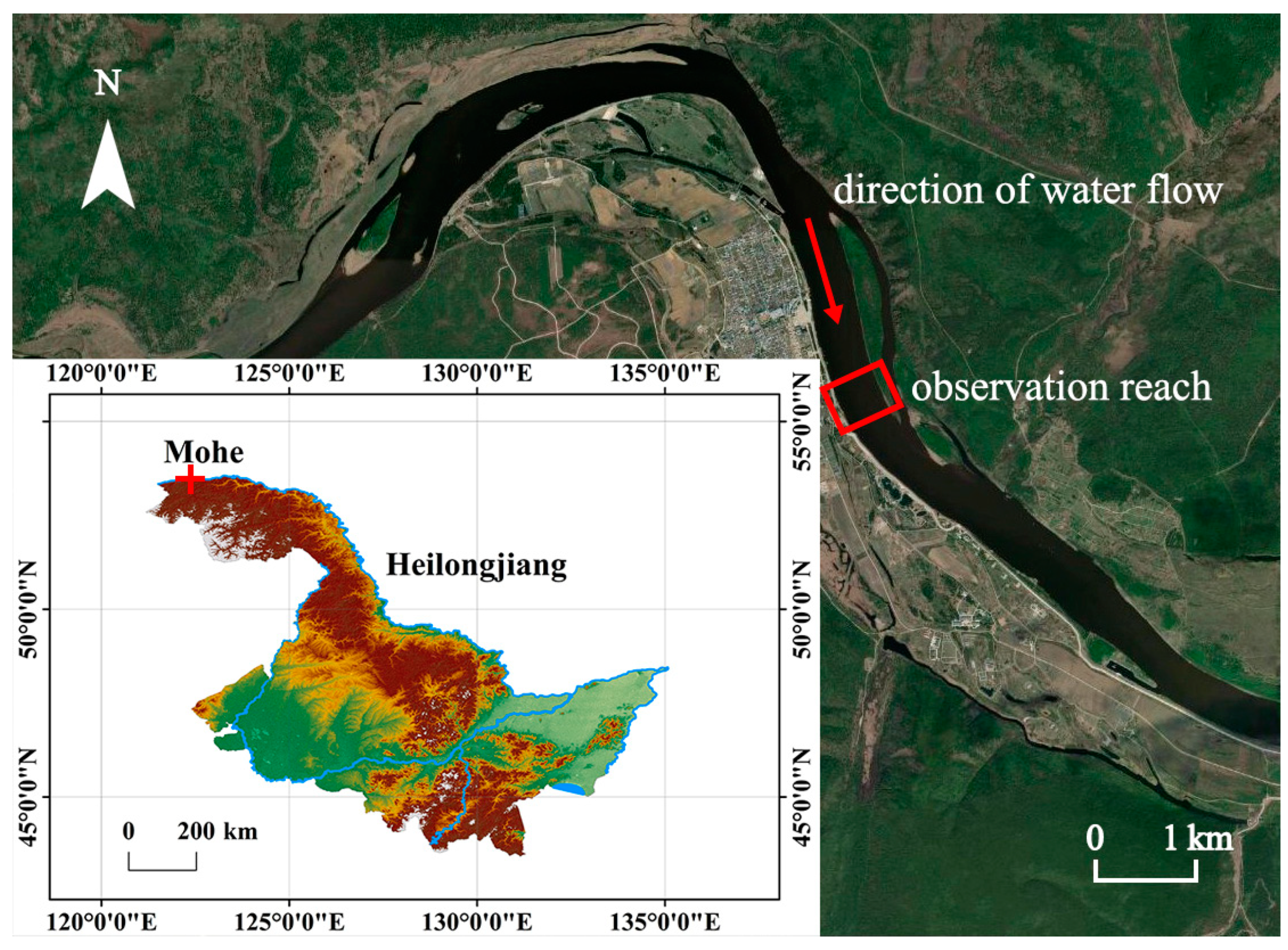
Figure 2.
Fitting curve between the unit pixel length and actual length in remote sensing images at the different heights.
Figure 2.
Fitting curve between the unit pixel length and actual length in remote sensing images at the different heights.

Figure 3.
Distribution of feature point pairs at 16:00 on 25 April 2021.

Figure 4.
Distribution of feature point pairs at 8:00 on 26 April 2021.
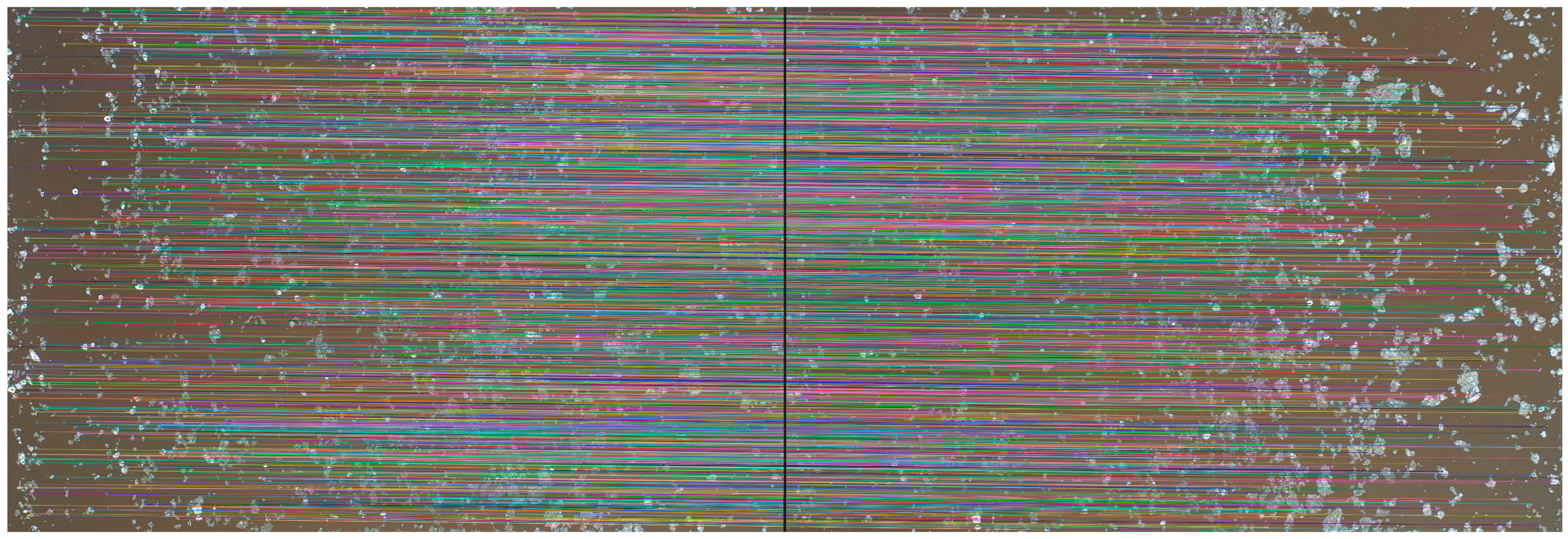
Figure 5.
Plane velocity field at 16:00 on 25 April 2021 (define the transverse pixel coordinate as x, and the longitudinal pixel coordinate as y, the coordinate directions are as shown in this figure).
Figure 5.
Plane velocity field at 16:00 on 25 April 2021 (define the transverse pixel coordinate as x, and the longitudinal pixel coordinate as y, the coordinate directions are as shown in this figure).

Figure 6.
Plane velocity field at 8:00 on 26 April 2021(define the transverse pixel coordinate as x, and the longitudinal pixel coordinate as y, the coordinate directions are as shown in this figure).
Figure 6.
Plane velocity field at 8:00 on 26 April 2021(define the transverse pixel coordinate as x, and the longitudinal pixel coordinate as y, the coordinate directions are as shown in this figure).

Figure 7.
Statistical histogram of ice plane velocity (a) 16:00, 25 April 2021; (b) 8:00, 26 April 2021.
Figure 7.
Statistical histogram of ice plane velocity (a) 16:00, 25 April 2021; (b) 8:00, 26 April 2021.
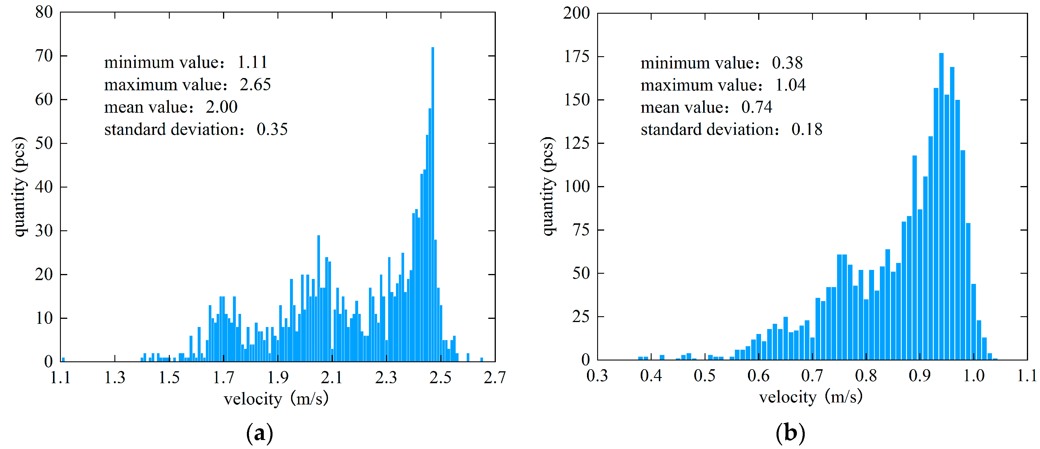
Figure 8.
Water level change chart.
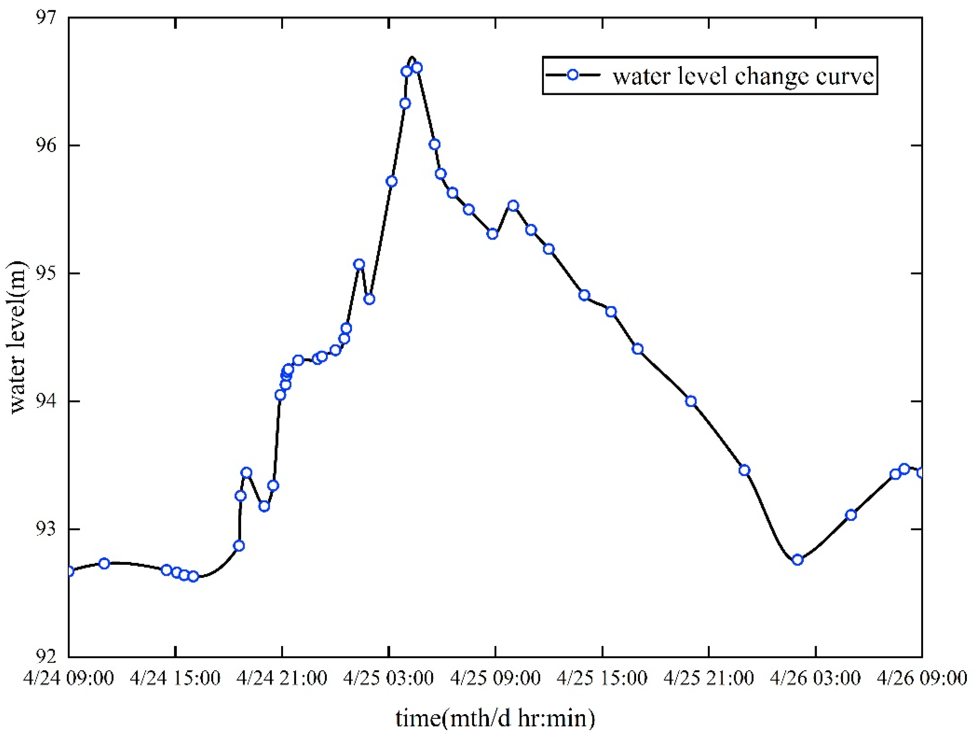
Figure 9.
Distribution law of ice velocity components: (a) the transverse components of the ice velocity at 16:00 on 25 April 2021; (b) the longitudinal components of the ice velocity at 16:00 on 25 April 2021; (c) the transverse components of the ice velocity at 8:00 on 26 April 2021; (d) the longitudinal components of the ice velocity at 8:00 on 26 April 2021.
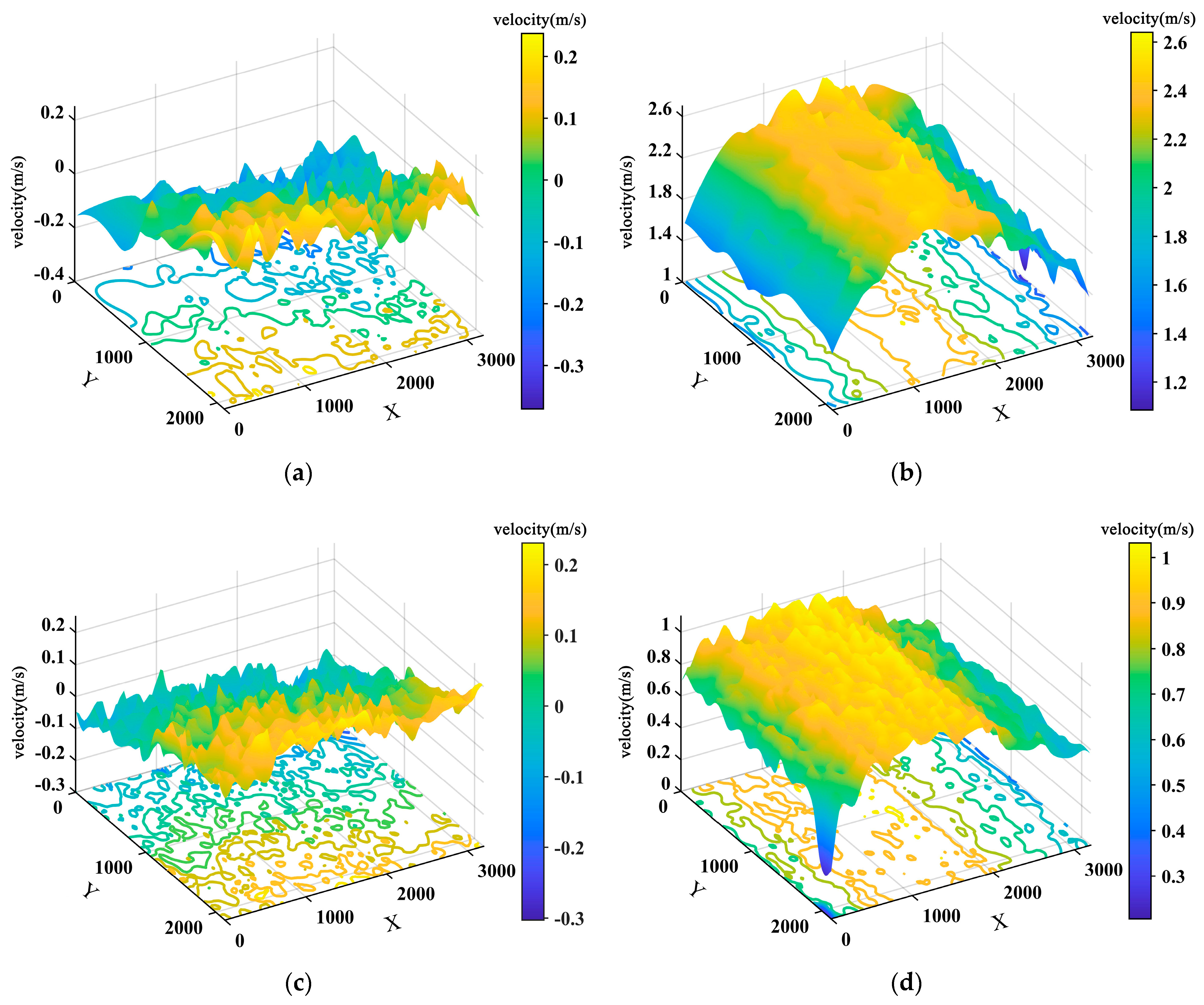
Figure 10.
The photo of the right bank (a) before ice flood period, (b) during ice flood period.
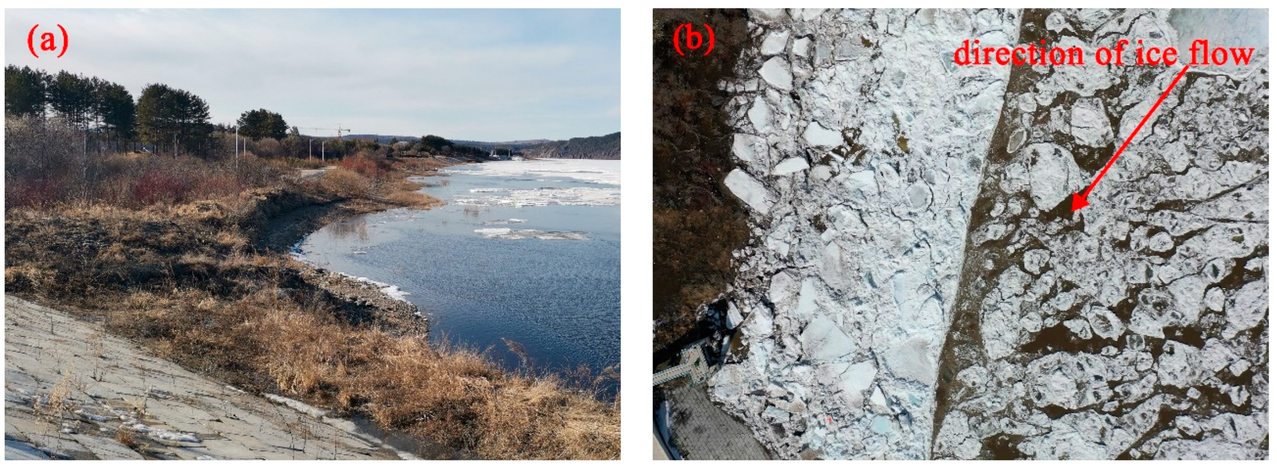
Figure 11.
Manual extraction of ice position: (a) original position of target ice at 10:28 on 2 May 2016; (b) position of target ice after 10 s [13].
Figure 11.
Manual extraction of ice position: (a) original position of target ice at 10:28 on 2 May 2016; (b) position of target ice after 10 s [13].
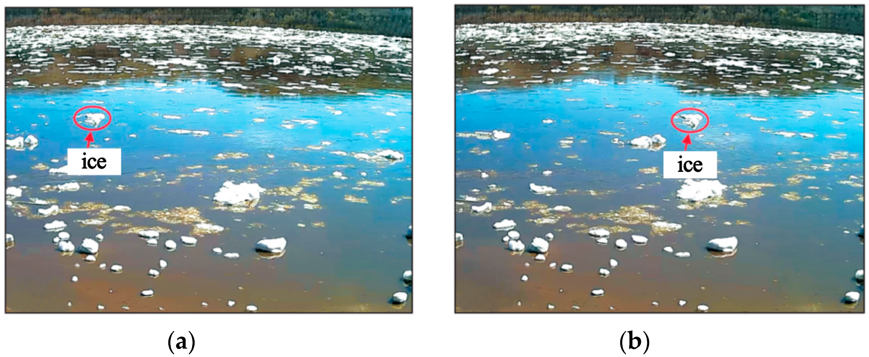
Figure 12.
Characteristic points on transverse section of the river channel.

Figure 13.
Comparison of plane velocity field based on SIFT algorithm and manual calculation: (a) 16:00, 25 April 2021; (b) 8:00, 26 April 2021.
Figure 13.
Comparison of plane velocity field based on SIFT algorithm and manual calculation: (a) 16:00, 25 April 2021; (b) 8:00, 26 April 2021.
Publisher’s Note: MDPI stays neutral with regard to jurisdictional claims in published maps and institutional affiliations. |
© 2022 by the authors. Licensee MDPI, Basel, Switzerland. This article is an open access article distributed under the terms and conditions of the Creative Commons Attribution (CC BY) license (https://creativecommons.org/licenses/by/4.0/).
Share and Cite
MDPI and ACS Style
Wang, E.; Hu, S.; Han, H.; Li, Y.; Ren, Z.; Du, S. Ice Velocity in Upstream of Heilongjiang Based on UAV Low-Altitude Remote Sensing and the SIFT Algorithm. Water 2022, 14, 1957. https://doi.org/10.3390/w14121957
AMA Style
Wang E, Hu S, Han H, Li Y, Ren Z, Du S. Ice Velocity in Upstream of Heilongjiang Based on UAV Low-Altitude Remote Sensing and the SIFT Algorithm. Water. 2022; 14(12):1957. https://doi.org/10.3390/w14121957
Chicago/Turabian StyleWang, Enliang, Shengbo Hu, Hongwei Han, Yuang Li, Zhifeng Ren, and Shilin Du. 2022. "Ice Velocity in Upstream of Heilongjiang Based on UAV Low-Altitude Remote Sensing and the SIFT Algorithm" Water 14, no. 12: 1957. https://doi.org/10.3390/w14121957
Note that from the first issue of 2016, this journal uses article numbers instead of page numbers. See further details here.