
A Python Application for Visualizing the 3D Stratigraphic Architecture of the Onshore Llobregat River Delta in NE Spain


1
Departamento de Álgebra, University of Granada, 18010 Granada, Spain
2
Departamento de Análisis Matemático, University of Granada, 18010 Granada, Spain
3
Departamento de Ciencias de la Tierra y Medio Ambiente, University of Alicante, 03080 Alicante, Spain
4
Departamento de Desertificación y Geo-Ecología, Estación Experimental de Zonas Áridas (EEZA–CSIC), 04120 Almeria, Spain
5
Instituto de Ciencias Químicas Aplicadas, Facultad de Ingeniería, Universidad Autónoma de Chile, Santiago 7500138, Chile
*
Author to whom correspondence should be addressed.
Water 2022, 14(12), 1882; https://doi.org/10.3390/w14121882
Submission received: 20 April 2022
/
Revised: 1 June 2022
/
Accepted: 8 June 2022
/
Published: 11 June 2022
(This article belongs to the Special Issue Coastal Aquifers Management: Hydrological, Environmental, Economic and Social Challenges in the Context of Global Change)
Abstract
:This paper introduces a Python application for visualizing the 3D stratigraphic architecture of porous sedimentary media. The application uses the parameter granulometry deduced from borehole lithological records to create interactive 3D HTML models of essential stratigraphic elements. On the basis of the high density of boreholes and the subsequent geological knowledge gained during the last six decades, the Quaternary onshore Llobregat River Delta (LRD) in northeastern Spain was selected to show the application. The public granulometry dataset produced by the Water Authority of Catalonia from 433 boreholes in this strategic coastal groundwater body was clustered into the clay–silt, coarse sand, and gravel classes. Three interactive 3D HTML models were created. The first shows the location of the boreholes granulometry. The second includes the main gravel and coarse sand sedimentary bodies (lithosomes) associated with the identified three stratigraphic intervals, called lower (>50 m b.s.l.) in the distal LRD sector, middle (20–50 m b.s.l.) in the central LRD, and upper (<20 m b.s.l.) spread over the entire LRD. The third deals with the basement (Pliocene and older rocks) top surface, which shows an overall steeped shape deepening toward the marine platform and local horsts, probably due to faulting. The modeled stratigraphic elements match well with the sedimentary structures reported in recent scientific publications. This proves the good performance of this incipient Python application for visualizing the 3D stratigraphic architecture, which is a crucial stage for groundwater management and governance.
1. Introduction
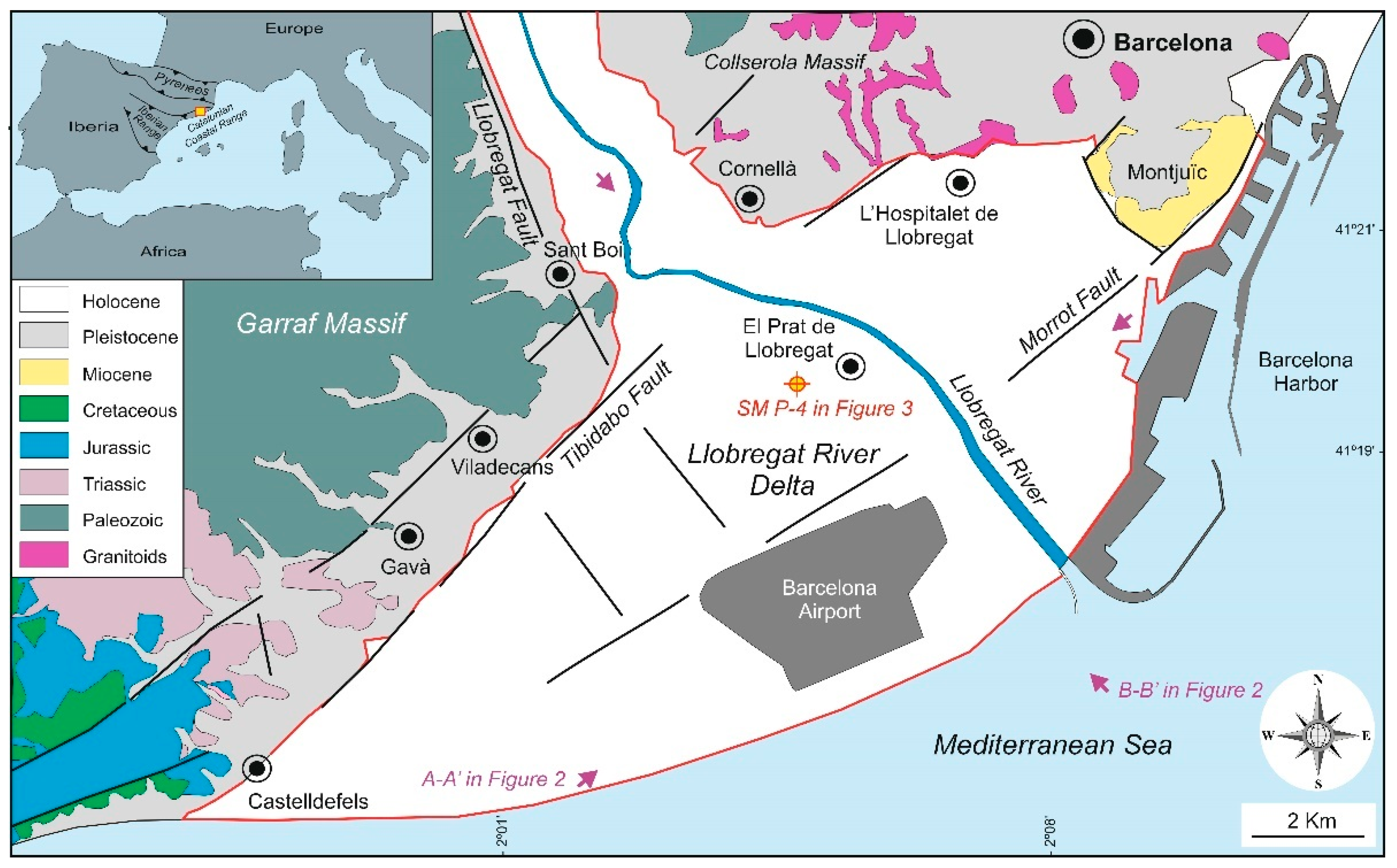
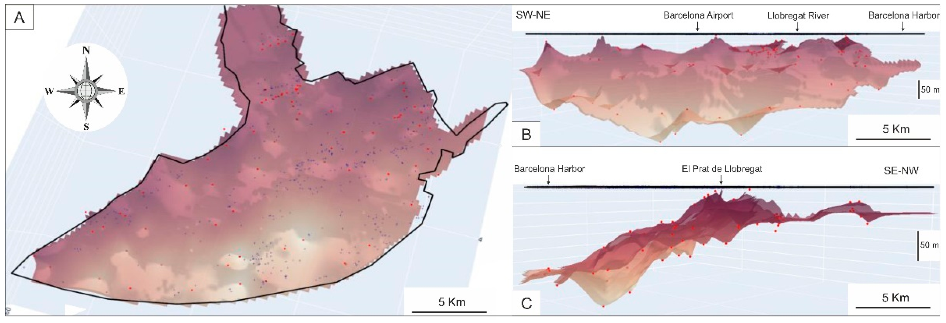
The Llobregat River Delta (LRD) is a densely populated coastal plain of 98 km2, forming the southwestern sector of the metropolitan area of Barcelona city in the Catalonia region in northeastern Spain (Figure 1). This area also includes other minor-order cities such as El Prat de Llobregat, L’Hospitalet de Llobregat, Cornellà, Sant Boi, Viladecans, Gavà and Castelldefels. The permanent surface-water provision and the abundance of groundwater have favored the development of coastal aquatic ecosystems and human settlements since ancient times. During the XIX and XX centuries, a large industrial activity developed in the area. Since the second half of the XX century, the high groundwater exploitation rates to supply to the increasing population and industrial activity produced negative consequences on groundwater quantity and quality, including seawater intrusion into aquifers and high levels of pollution [1]. Other modern development milestones occurred in Barcelona city and its metropolitan area, such as the Olympic Games in 1992 and the Llobregat Delta Infrastructure and Environment Plan (Pla d’Infraestructures i Medi Ambient del Delta del Llobregat, PDL) started in 1994 [2] have modified the LRD land use and geomorphology. The PDL included large civil infrastructures with variable underground development such as the extension of the International Airport and Harbor of Barcelona, a dense network of new highways, different underground lines, conventional and high-speed railways, wastewater new treatment plants, desalination plants, diversion of the Llobregat River final section, and many other civil works.
The PDL was a disruptive milestone in what concerned the generation of new, testable geological and hydrogeological information. The conventional geotechnical exploration data for designing civil work foundations and the drilling of dozens of boreholes to monitor the impacts of civil works on groundwater provided huge, detailed geological and hydrogeological data. In 2004, the Water Authority of Catalonia (Agència Catalana de l’Aigua, ACA) created the Technical Unit of the Llobregat Aquifers (Mesa Tècnica dels Aqüífers del Llobregat, METALL). This Hydrogeological Research Unit was devoted to compiling and homogenizing the former and new (in production) geological and hydrogeological information in order to prepare groundwater flow numerical models aimed at assessing the cumulative impact of the large civil works on the groundwater bodies [3]. Nowadays, the ACA manages this public geological and hydrogeological database, which is available on request.
From a geological point of view, the LRD is regionally fed by the Llobregat River and its tributaries arriving from the Pre-Pyrenean Range and locally from the Llobregat River lower valley reliefs (Garraf and Collserola massifs) belonging to the Catalonian Coastal Range [4,5]. This range is a NE–SW-oriented mountain chain that gives pass downward to the Mediterranean coast (Figure 1). In the LRD, the geological studies started at the end of the XIX century by Almera [8]. In the XX century, several studies [4,5,6,9,10] allowed proposing geological maps and 2D cross-sections aimed to support hydrogeological studies. Sedimentological studies performed in the 1970s and 1980s [11,12,13] allowed clarifying the geology of the LRD. In the 1980s, the prodeltaic bodies of the emerged delta, dated as Holocene, were studied in detail [14] and the geological characterization of the continental shelf with support of 2D marine seismic reflection took place [12,13,15]. These studies, with a strong sedimentological component, allowed the sequential division of the LRD and the arrangement of the Quaternary materials. In the 1990s, this huge geological background was combined with the former geological information compiled from dozens of boreholes to make modern groundwater evaluations [16]. Coinciding with the PDL development at the beginning of the XXI century, new geological data allowed fine research [7,17,18,19,20] aimed to detail the 2D stratigraphic architecture of the LRD, thus giving a response to the Pliocene–Quaternary boundary, the confident definition of those detritic levels officially cataloged as productive, high-yielding aquifers and the detailed identification of those interconnected stratigraphic structures (of sedimentary and tectonic origin) through which seawater intrusion into aquifers and mobilization of pollutants take place.
In recent times, numerical modeling has progressively been employed to characterize the geometry of geological structures and sedimentary bodies (lithosomes). Numerical tools involve a variety of deterministic and stochastic models, as well as geostatistical and geospatial techniques. The choosing criteria depend on the purpose of the research, input data typology and spatial coverage, and capability for calibrating and validating predictions. Regarding the interpolation tools, this field of research allows the 3D mapping of certain physical parameters controlled by sedimentary processes that determine the hydraulic behavior of the geological reservoir. The 3D mapping allows better visualizations than the classic 2D serial cross-sections [21,22,23,24]. A variety of software for 3D visualization based on different interpolation algorithms is available. Commercial tools such as MOVE (Petroleum Experts Ltd., Edinburgh, UK), 3D Geomodeller (Intrepid Geophysics, Brighton, Australia), Autocad Civil (Autodesk, Inc., San Rafael, CA, USA), Gocad (Emerson Paradigm Roxar), ArcGis, PETREL (Geology and Modeling from Schlumberger), VOXI (Earth Modeling from Geosoft) and Geoscene 3D (I-GIS) are available for 3D geological visualizations. There are other open-source applications such as Gempy or OSGeo. The Gempy applications have proven to be accurate enough and have technical support for users, but they are expensive. The advantage of OSGeo applications is the zero cost and adaptability (modifying or extending the sources), but the absence of technical support for users and sometimes low reliability are its negative parts. There are commercial and open-source libraries devoted to geographic information systems (GIS) and mapping. For instance, there are Python libraries [25,26,27] and posts listing libraries [28,29] for different geological interests, including structural geology, sedimentology, mining, and hydrogeology. There are also scientific documents where computer tools are developed or applied to different fields of geology [30,31,32,33]. In addition, some social media channels have also posted data analytics and machine learning educational applications focused on geology [34].
The experience of the mathematician researchers involved in this paper with Python for data handling and 3D mapping was an advantage for adapting this knowledge to geological concepts and concerns. This adaptation required less effort than learning specific tools developed for geologists. So, this paper introduces a Python application for visualizing the 3D stratigraphic architecture. The application interpolates the parameter granulometry deduced from borehole lithological records to create interactive 3D HTML models of essential stratigraphic elements. For this, the application uses different Python packages, including basic interpolation and shape algorithms. On the basis of the high density of boreholes and the subsequent geological knowledge gained during the last six decades, the Quaternary onshore LRD was selected to show the application. The public geological and hydrogeological database managed by the ACA was consulted to compile the information used in this paper, i.e., the granulometry dataset generated by METALL.
Different research disciplines in Earth and Environment Sciences require 3D visualization of available geological information. As described above, the LRD is a strategic coastal aquifer whose sustainability is threatened by strong human pressure. In this case, the Python application may assist to drill proper pumping wells and optimize groundwater monitoring networks, as well as evaluating how the large civil works may impact the groundwater resources. The spatial distribution of granulometry will also be of assistance to design compensatory measures for aquifer protection and recoveries such as artificial aquifer recharge and positive hydraulic barriers to reduce the advance of seawater intrusion and mobilization of pollutants.
Appendix A includes the four Jupyter notebooks describing the data handling and 3D mapping. An operative version of the introduced Python code can be downloaded from the GitHub repository described in Supplementary Materials. The results of this Python application are HTML files that do not require any additional tools apart from a web browser to view different perspectives, hide elements, enlarge or focus on specific areas or elements and take snapshots of a particular view. These actions can all be performed using just a mouse.
2. Geological and Hydrological Setting
The LRD is located at the foot of the Catalonian Coastal Range (Figure 1). In the area, this mountain range includes rocks of Paleozoic (granites and slates) and Mesozoic (Triassic conglomerates, sandstones, and pelites; Jurassic dolostones and limestones; Cretaceous marly limestones). The LRD is NE bounded by the Montjuïc Mount (Figure 1) made of Miocene calcarenites and marly limestones [17]. This area represents a Neogene rifted margin associated with the opening of the Valencia Trough and is affected by several fault families (Figure 1) probably active and mainly oriented NE–SW (Morrot and Tibidabo fault families) and NW–SE (Llobregat fault family), that conditioned the main reliefs and the location of the Llobregat River outlet [7].
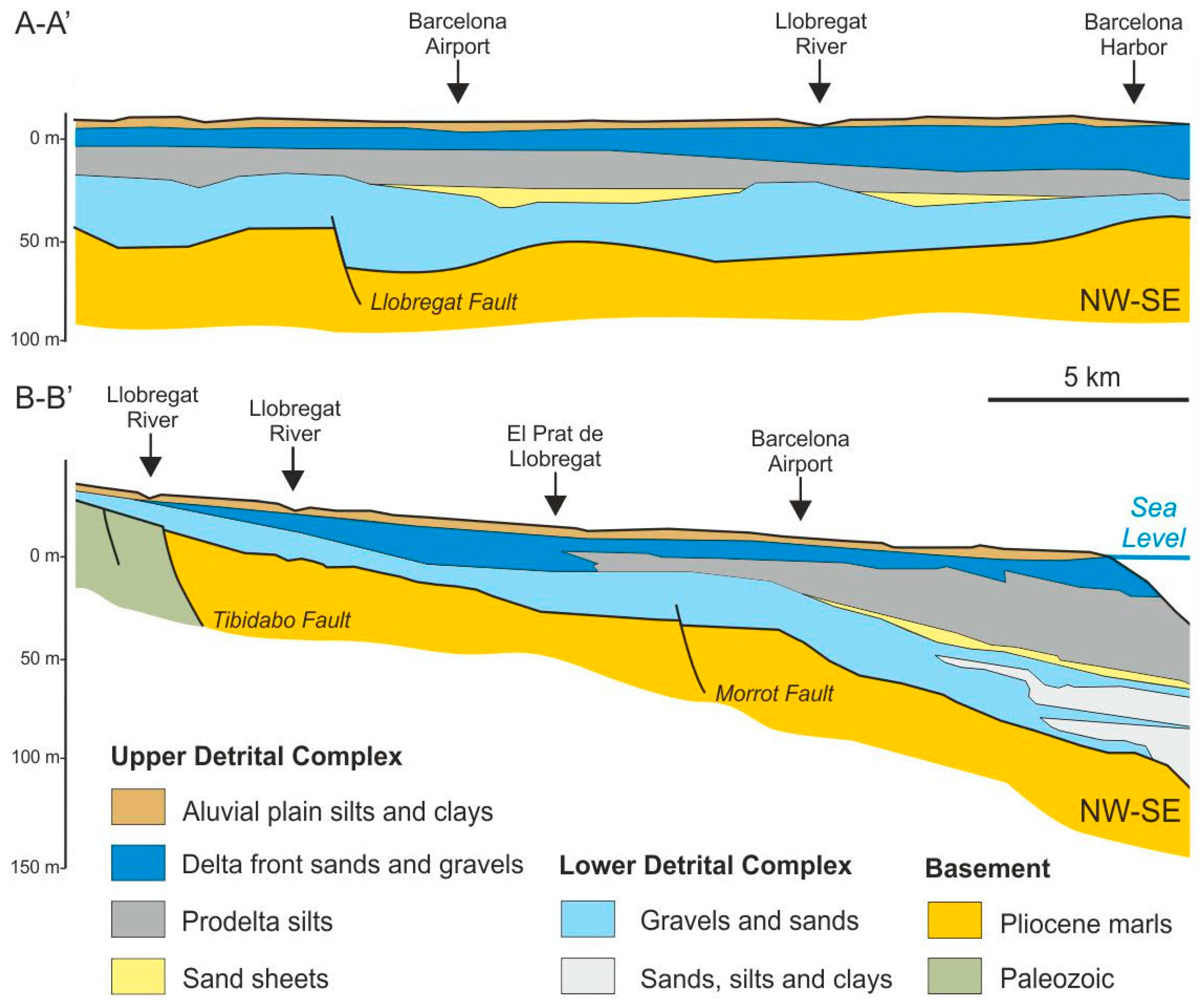
With respect to the LRD formations (Figure 2), Pliocene and older rocks are considered the basement, which is separated from the Quaternary formations by an important unconformity surface [18]. Pliocene substratum is made of estuarine marls, silts, and clays [12,13,17]. The Quaternary record was divided into two depositional sequences Pleistocene and Holocene in age [7,12,13,17,18,20]. The terms upper detrital complex and lower detrital complex have also been used [7] for the same depositional sequences (Figure 2). According to geophysical studies in the offshore delta in the marine platform [12,13], the lower detrital complex can be divided into three parasequences [7]. In general terms, the lower detrital complex is made of conglomerate bodies (locally with sand) with intercalated silt- and clay-rich intervals [12,13,35]. The upper detrital complex, from bottom to top, is made of a sand layer, a silt bed, gravel (locally with sand), and upper silt and clay cover forming the current alluvial plain and the associated coastal wetlands and marshes [11,35].
From a hydrological point of view, the Llobregat River basin spans from the Pyrenees (the mountain range located between Spain and France; Figure 1) to the Mediterranean Sea with a total length of 170 km and covering around 4950 km2 [20]. The Llobregat River shows an irregular streamflow regime in the 250–1500 Mm3 range determined by a Mediterranean-like climate regime [11]. The deltaic plain is also modeled by several ephemeral streams coming from the Garraf and Collserola massifs [17]. Apart from this hydrological control, the LRD coastal fringe has also been modified by the regional littoral drift towards the SW. In this area, littoral currents of about 30 cm s–1 redistribute the sediments to the SW also bringing sediments from northern rivers and streams [36,37]. To a lesser extent, the waves (low energy) and the tide (a few centimeters) contribute to the sediment’s redistribution in the coastal areas of the LRD [36,37].
3. Materials and Methods
3.1. Python Programing Language
The object-oriented, high-level Python programming language [38] was used for granulometry data treatment and displaying the 3D HTML models of essential stratigraphic elements. Python is an open-source language used in many environmental topics, including geological ones. Many packages or modules use this programming language for a wide variety of problems. The Python packages used here were (i) NumPy [39] for data computing, (ii) Pandas [40] for data analysis and processing, (iii) Plotly [41] as a plotting library, (iv) UTM [42] to deal with UTM coordinates and borehole prospecting depths, and (v) Scipy [43] for interpolation and render algorithms.
3.2. Data Compilation and Pretreatment
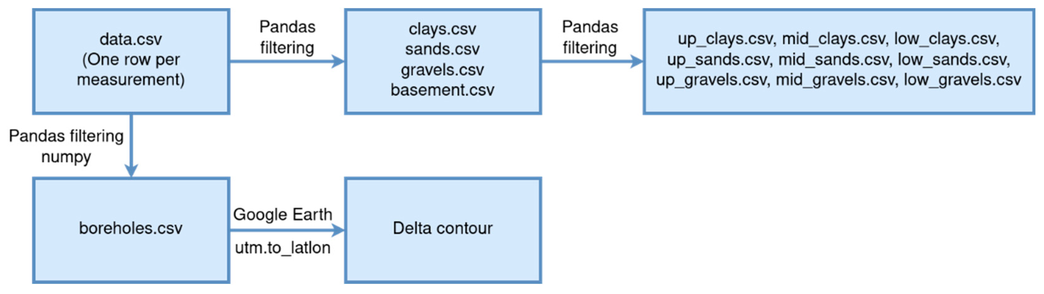
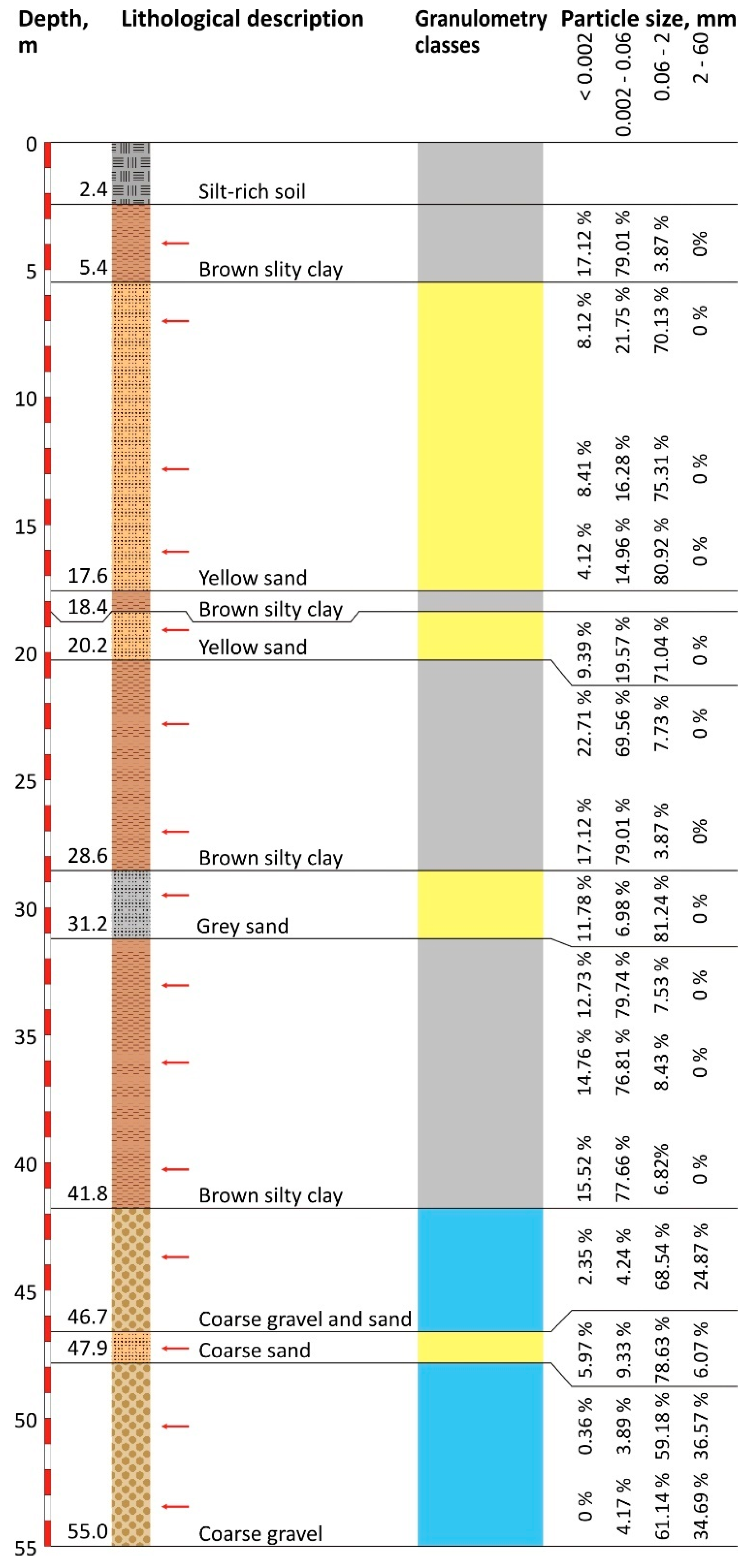
The public geological and hydrogeological database managed by ACA was consulted to compile the lithological records of 433 boreholes in the onshore LRD, which can be also downloaded from Alcalá et al. [44], and the granulometry dataset generated by METALL from both Lab tests values and proxy values after visual recognitions of the predominant lithologies, which is available on request. The geotechnical borehole SM P-4 (located in Figure 1) with granulometry data is included in Figure 3 as an example. The dataset consisted of georeferenced XLS (Excel) files with meter-by-meter granulometry values associated with the boreholes lithotypes. The boreholes’ location (coordinates x and y) and prospecting depth (coordinates z) lead to a georeferenced array of granulometry data associated with the prospected lithologies over space and depth (Figure 4).
Figure 3.
A selected geotechnical borehole (SM P-4, location in Figure 1), showing the granulometry tests (red arrows) performed through the Spanish standards and their results for gravel (cyan), coarse sand (yellow), and silt–clay (gray) granulometry classes. This information forms part of the granulometry dataset generated by the METALL used in this paper.
The georeferenced granulometry dataset and the original boreholes lithologies [44] were additionally compared to detect possible outliers. After checking, the georeferenced granulometry data were clustered into three main granulometry classes: clay–silt (<1 mm), coarse sand (1–5 mm), and gravel (>5 mm). Although expandable because Pandas can handle XLS files directly, data conversion to CSV format for further processing with Pandas has been preferred. The CSV files are easier to handle using a plain text editor only, so the users can use Pandas or just a plain text editor to make data edits needed.
3.3. The 3D Mapping of the Boreholes Granulometry Classes
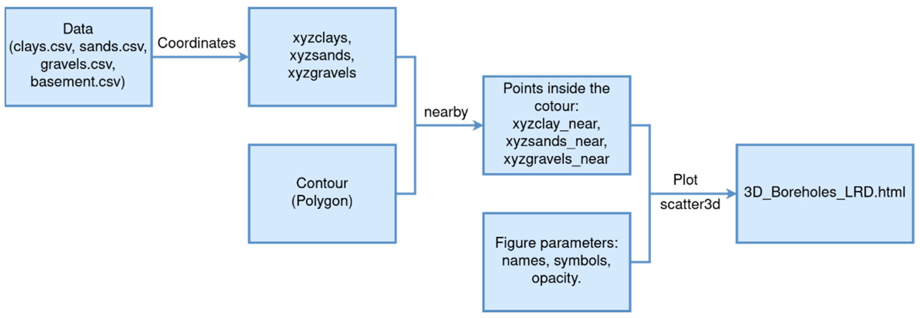
Python has different visualization libraries, and Plotly [40] is one of them. Plotly was chosen because it is a web-based tool kit that can be accessed from a Python Notebook. The Plotly function Scatter3d was used for mapping boreholes. The use of this function requires additional data processing.
First, the function coordinates (data, positions) were defined. This function (i) lists the X, Y, and Z UTM coordinates extracted from ‘data’ by looking at the data indicated at ‘positions’, and (ii) models the data in legible format by the Scatter3d function. However, only the boreholes inside the LRD contour are needed. The function near (xyz,polyg,dis) is defined to select these boreholes. This function uses the Python Geometry function ‘distance’ to select coordinates within a distance less than ‘dis’ from the polygon ‘polyg’ in the ‘xyz’ list. Once these data are obtained in the required format, the Plotly function Scatter3d is used to create the figure. Some parameters such as the symbol, size, and opacity of the borehole, thickness and type of the LRD contour, and figure limits must be chosen. The aspect ratio determines the proportion of the Z axis regarding the X and Y axes, thus allowing the exaggeration of the Z scale for better displaying. This ratio must also be defined. This working flow is synthesized in Figure 5. Appendix A and the Jupyter notebook boreholes_3D_map.ipynb hosted in the GitHub repository described in Supplementary Materials include the complete code.
3.4. The 3D Mapping of the Stratigraphic Architecture
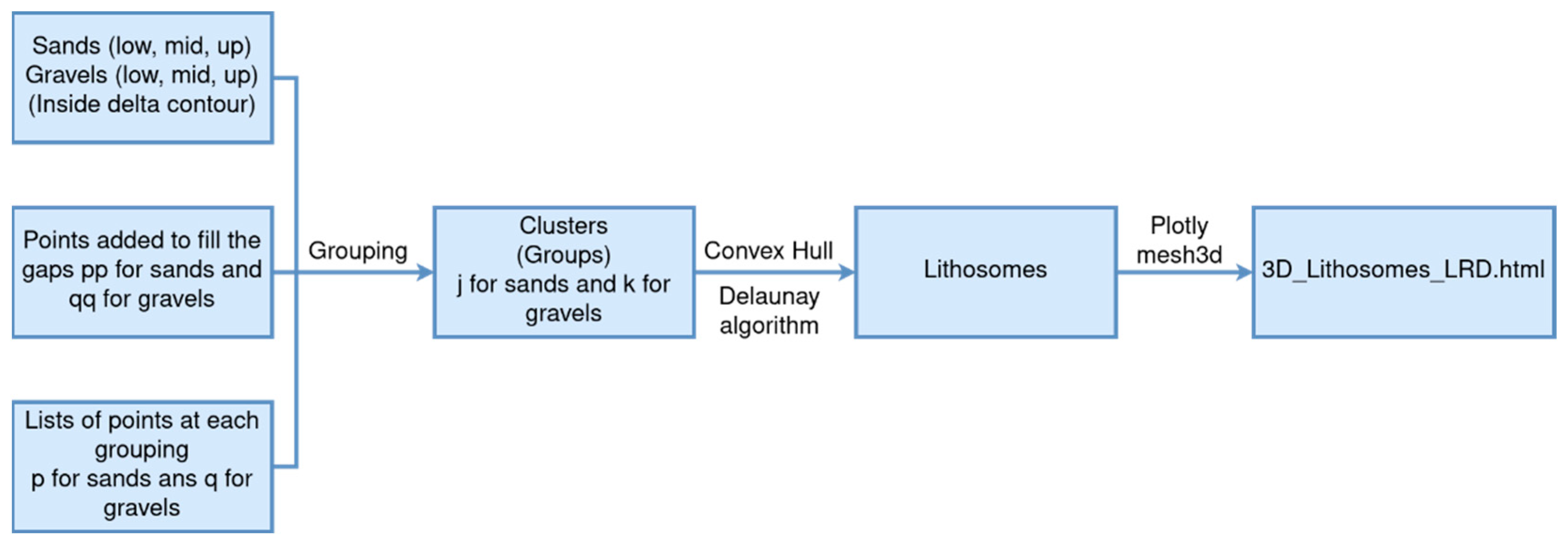
Due to the hydrogeological interest of the LRD, we decided to focus the study on the gravel and coarse sand lithosomes forming the local aquifers (Figure 6). When checking the borehole lithosomes (3D_Boreholes_LRD.html), gravel and coarse sand lithologies appeared concentrated preferably in certain zones of the top, middle and low levels. Then, a list of points (q_up, q_mid, and q_low for gravel, and p_up, p_mid, and p_low for coarse sand) with a representative point in each zone with a predominant granulometry was defined. A mathematical strategy (nucleation-like) is further used to create (and shape) the lithosomes associated to a given granulometry class (quasi-equal granulometry lithosomes). The mathematical strategy involves a function named grouping that depends on two auxiliary functions named within and within2. The function within (p,list,n) depends on three parameters: a point ‘p’, a list of points ‘list’, and a number ‘n’. This function is defined in plain Python (does not need to use NumPy functions) and just selects the elements of the variable list located within a distance n of the point p. The other within2 (list1,list2,n) function, also defined in plain Python, applies the function within (p,list2,n) for each p in list1 and puts the selected elements in the return list. Finally, the grouping (list1,list2,n) function recursively uses the within2 function to return a list with all elements in the variable list2 located within distance n of any element that is itself within distance n of each given point in the variable list1. This third function is also defined in plain Python.
Clearly, the efficiency of this function grouping is improvable, since its recursive nature implies repeating the same calculation many times, but its definition is very simple, and it does the job. Nevertheless, the lack of information between boreholes forces us to manually infer the lithological type in those blank spaces. To solve this gap, we add two lists (qq for gravel and pp for coarse sand) to the original data at each level. This makes the grouping strategy work properly.
Once the granulometry data of each lithosome were grouped by using the above nucleation strategy, the elements forming the previously defined groups of each lithosome were computed. For this, the Convex Hull algorithm developed by the SciPy community [44] was implemented. The 3D convex hull of a georeferenced dataset is the smallest polyhedron that wraps up all of them. The convex hull function must be applied to each obtained lithosome. The Delaunay triangulation algorithm [45] is used to render the shape of the lithosomes.
Finally, the ‘Mesh3d’ Plotly function was implemented to draw the volume figure, named 3D_Lithosomes_LRD.html. The output is an interactive 3D HTML model that (i) can be opened with any browser and (ii) allows observing different views of the mapped lithosomes, zooming, rotating, and moving around, as well as hiding any of them by clicking in the proper element in the right-side legend. This working flow is synthetized in Figure 6. Appendix A and the Jupyter notebook boreholes_3D_map.ipynb hosted in the GitHub repository described in Supplementary Materials include the complete code.
3.5. The 3D Mapping of the Basement Top Surface
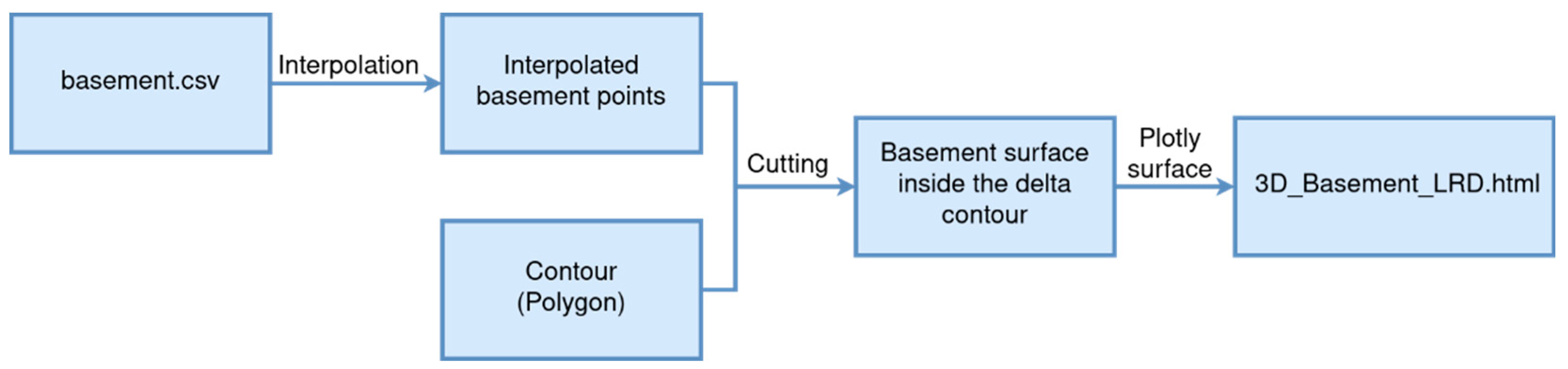
A basic inverse distance weighted (IDW) interpolation algorithm was implemented to map the basement top surface (Figure 7). This IDW spatial function was obtained from the GEODOSE block, which can be found in the 3D terrain modelling package on the Python website [46]. To run this spatial function, a maximum data searching over a maximum searching distance (in both x, y, and z coordinates) was imposed, taking the boundaries imposed by the onshore LRD contour (x and y coordinates) and basement depth (coordinate z is the basement first-prospecting depth) into account. The first step was selection of those boreholes reaching the basement within the onshore LRD contour. This information was gathered from the CSV files to predict (by using the IDW spatial function) the continuous basement top surface shape.
The mapping grid has to be chosen in such a way that the computing time will be reasonable, and the result obtained was geologically sound. For this, it is important to choose a proper iteration radius (block radius) and the p-value ‘p’ for the weight that the IDW spatial function uses. Using the selected mapping grid, the Plotly function surface is implemented to draw the basement top surface.
The output is an interactive 3D HTML model that can also be opened with any web browser and allows observing different views and details of the mapped basement top surface. This working flow is synthetized in Figure 7. Appendix A and the Jupyter notebook boreholes_3D_map.ipynb hosted in the GitHub repository described in Supplementary Materials include the complete code.
4. Results
4.1. The 3D Mapping of the Boreholes Granulometry Classes
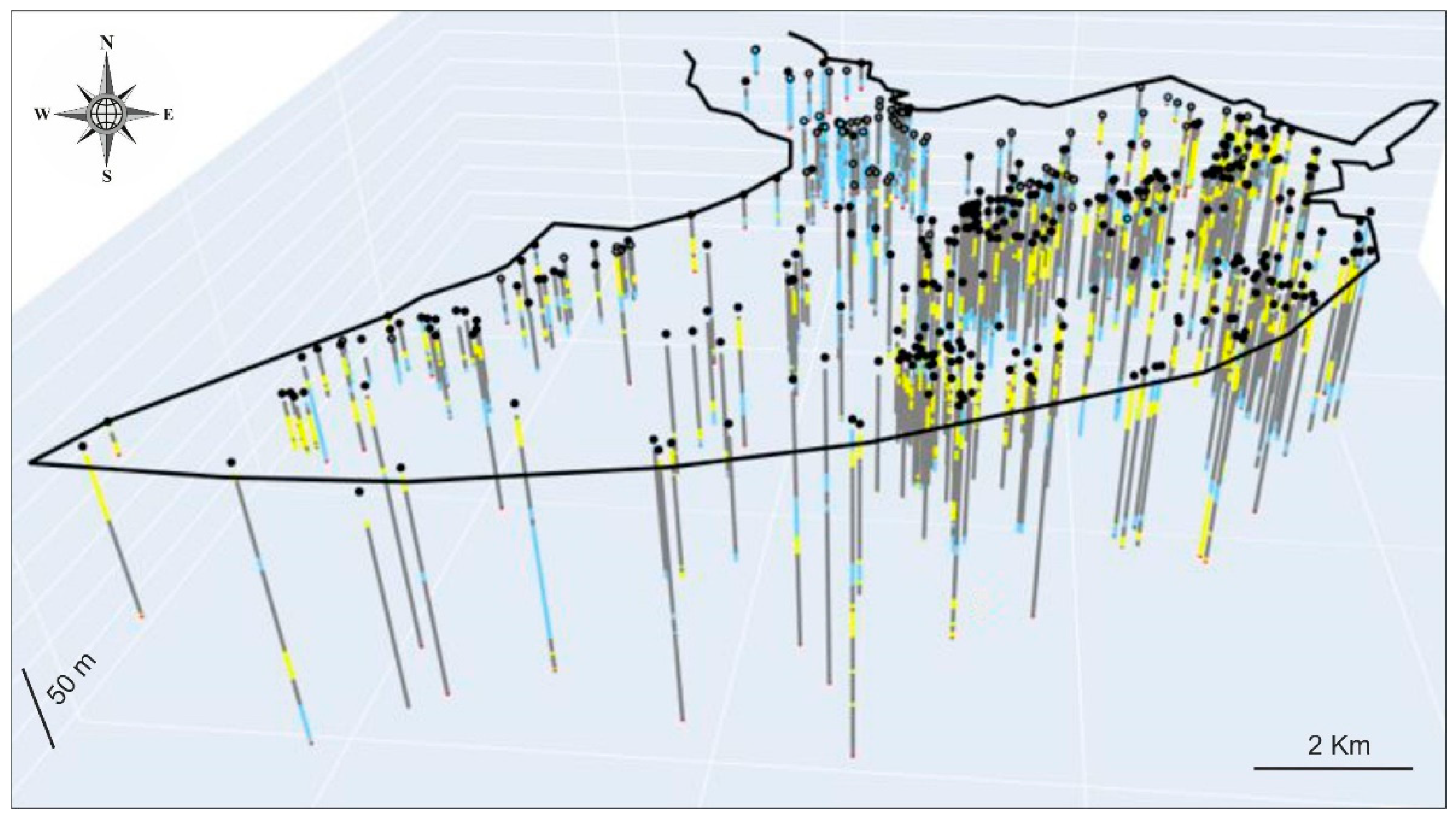
Figure 8 shows the 3D HTML model created to display the 3D distribution of the granulometry classes along the Z axis in each of the 433 boreholes complied in the onshore LRD. An interactive 3D HTML version of this model (3D_Boreholes_LRD.html) is provided as supplementary material. The plotting adopted a 1:1:50 (x = 2, y = 2, and z = 0.5) aspect ratio because of the thinness of the LRD Quaternary record regarding the x and y distances. This 3D view allows identifying three intervals where coarse detritic rocks (gravel and coarse sand) are concentrated and separated by other intermediate fine detritic intervals (silt and clay) as (i) >50 m b.s.l. lower interval (b.s.l. means below sea level), (ii) 20–50 m b.s.l. middle interval, and (iii) <20 m b.s.l. upper interval. Moreover, this 3D view also allows defining several bodies grouping the main gravel and coarse sand lithosomes. These stratigraphic intervals including the lithosomes were proposed by standard stratigraphic correlation procedures.
4.2. The 3D Stratigraphic Architecture of the Quaternary Coarse Detritic Lithosomes
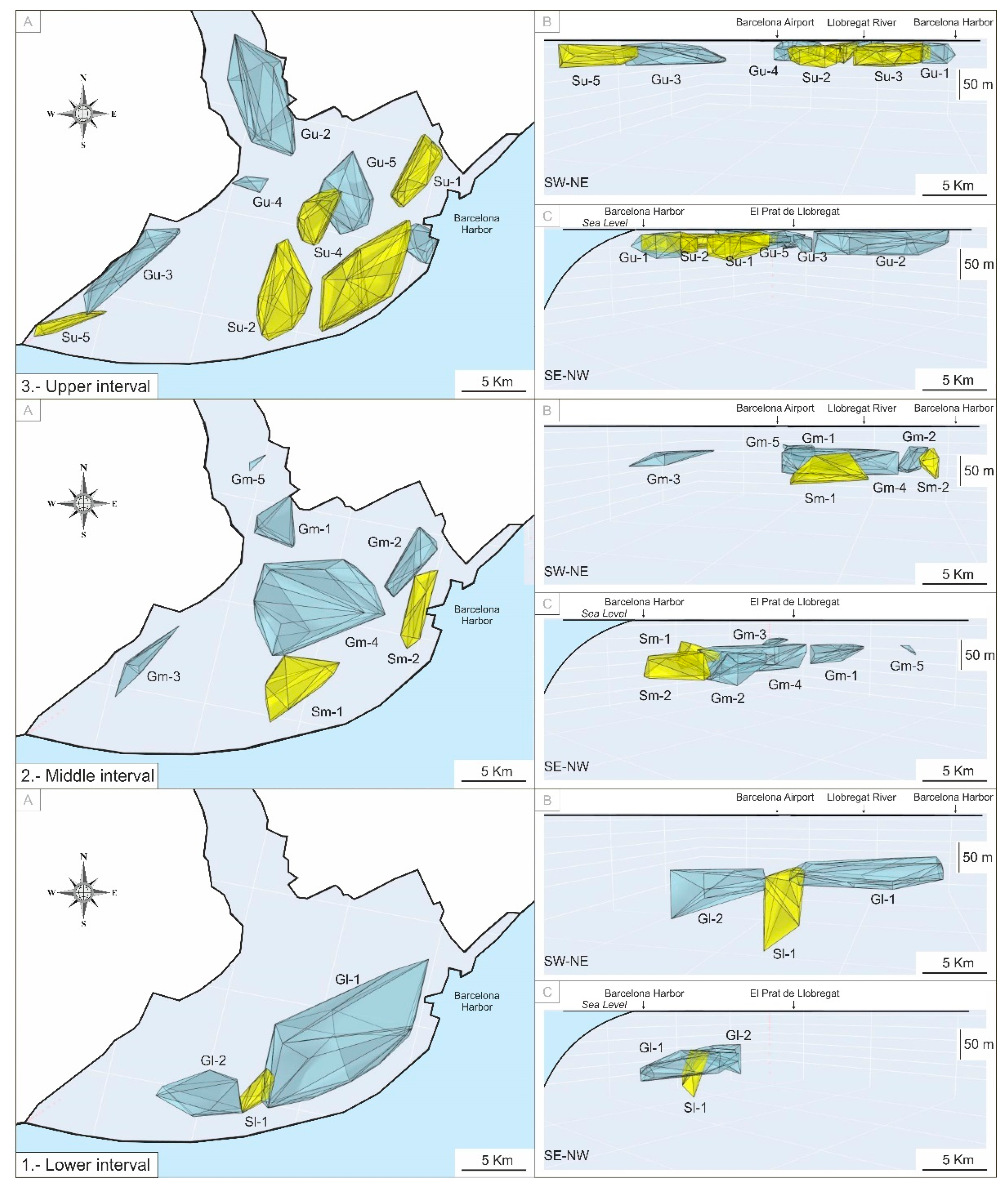
Figure 9 shows the 3D HTML model created to display the 3D distribution of the gravel (G) and coarse sand (S) lithosomes within the onshore LRD lower (l), middle (m), and upper (u) intervals. An interactive 3D HTML version of this model (3D_Lithosomes_LRD.html) is provided as supplementary material. The plotting adopted a 1:1:50 (x = 2, y = 2, and z = 0.5) aspect ratio to show three different zenithal, SE–NW frontal, and NE–SW lateral frontal views of the lithosomes, which are labeled as Gl-1 and Gl-2 for the gravel lithosomes of the lower interval, Sl-1 for the coarse sand lithesome of the lower interval, Gm-1 to Gm-5 for the gravel lithosomes of the middle interval, Sm-1 and Sm-2 for the coarse sand lithosomes of the middle interval, Gu-1 to Gu-5 for the gravel lithosomes of the upper interval, and Su-1 to Su-5 for the coarse sand lithosomes of the upper interval. The dark gray lines are rendering effects of the implemented Delaunay triangulation algorithm to improve the shape of the lithosomes volumes and highlight the faces of the convex hulls.
4.3. The 3D Mapping of the Basement Top Surface
The basement top surface is an important stratigraphic element that determines the accommodation space for the Quaternary sedimentation. Within the onshore LRD contour, a total of 87 boreholes reaching the basement were gathered from the CSV files to predict (by using the IDW spatial function) the continuous 3D basement top surface. Taking the 98 km2 onshore surface of the LRD into account, after several trials, the optimal regular mapping grid was 100 m × 100 m (n = 100), the block radius was 5 (r = 5), and the p-value was 2 (p = 2). Figure 10 shows the 3D HTML model created to display the 3D mapping of the basement top surface. An interactive 3D HTML version of this model (3D_Basement_LRD.html) is provided as supplementary material. The plotting adopted a 1:1:50 (x = 2, y = 2 and z = 0.5) aspect ratio to show three different zenithal, SE–NW frontal and NE–SW lateral frontal views. This model also allows different views, zooming, rotating, and moving around, as well as hiding elements to focus on details.
5. Discussion
From the above-introduced methodology and the scope of the achieved stratigraphic applications, several novel subjects can be discussed. First, the Python application seems to be an ergonomic and easy-access tool for visualizing the 3D stratigraphic architecture. The 3D models can be viewed in a web browser, so they are easily accessible to every user. The interactive 3D HTML models of essential stratigraphic elements (volumes and surfaces) allow for making quantitative measures, which is quite valuable to support many applied hydrogeological, geotechnical, and mining research interests. The second is the use of the granulometry as basic interpolating data (Figure 3), which is of special interest for geological explorations of porous sedimentary media because this physical parameter determines the storage of a fluid and its ability to move through the pores, including groundwater, oil, gas, brines, leachates, and pollutants. The third is related to a research gap concerning the need to program additional routines to assess the 3D models’ uncertainty, which is a task currently ongoing.
Regarding the Quaternary stratigraphic architecture and basement surface of the onshore LRD, additional findings to the above-described geological model have been obtained. For instance, the gravel and coarse sand lithosomes seem to be arranged into three stratigraphic intervals called lower (>50 m b.s.l.), middle (20–50 m b.s.l.), and upper (<20 m b.s.l.), as reflected in Figure 9. These coarse lithosomes seem to be deposited showing the following trend: in the distal LRD sector in the lower interval, in the central LRD sector in the middle interval, and in the entire LRD but with a great gravel lithosome in the embedding of the Llobregat River between the Garraf and Collserola massifs in the upper interval. This evolution fits well with the recent scientific literature (reflected in the lower cross-section in Figure 2) and seems to indicate a transgression during the lower and middle intervals with progressive retreating of coarse deposits towards proximal areas (getting closer and closer to the Garraf and Collserola massifs). This would be followed by a rapid regression with a spreading of coarse deposits toward distal areas to occupy the entire LRD. Figure 9 shows how the coarse deposits are not homogeneous in the entire LRD, as the old cylindric interpretation from the scientific literature indicated [11,35]. On the contrary, they fit very well with the recent interpretations, in which more parasequences with discontinuous coarse sedimentary bodies spread over the entire LRD were defined [7].
With respect to the basement, which is mostly composed of Pliocene rocks and Miocene and Paleozoic rocks to a minor extent [12,13,17], the different 3D views show a very irregular top surface. Figure 10 shows an overall steeped ‘horsts-grabens’ structure deepening toward the marine platform. This overall trend is interrupted with a raised (horst) sector in the El Prat de Llobregat town area, probably due to faulting, which is clearly visible in Figure 10C. In fact, when Figure 10C is compared to Figure 1, this horst sector narrowly coincides with the prolongation of the Montjuïc Mount elevation due to the action of the Morrot faults family below the LRD. The prolongation of the Tibidabo, Llobregat, and Morrot fault families could also explain the ‘horsts-grabens’ structure in the basement top surface of the onshore LRD in good agreement with recent research [7,47].
6. Conclusions
In 2004, the ACA created the METALL to compile and homogenize geological and hydrogeological information in order to assess the cumulative impact of the PDL civil infrastructures (with variable underground development) on the LRD groundwater bodies. On the basis of the high geological knowledge gained about the Quaternary onshore LRD, this area was selected to show the performance of a Python application that implements the packages NumPy, Pandas, Plotly, and Scipy for visualizing the 3D stratigraphic architecture. Although there are many commercial and open-source libraries and software devoted to geological visualization, its use often requires effort to learn how they work and money in the case of the commercial ones. The use of the Python language has proven efficient, ergonomic, and easy access to the results.
The Python application uses the granulometry dataset deduced from 433 borehole lithological records as interpolating data to create interactive 3D HTML models of essential stratigraphic elements. These models can be viewed in a web browser without any additional tools, so they are easily accessible to every user. The users can make different views, zoom, and move around, as well as hide any element by clicking that element in the right-side legend to see other details. The current development stage of the application enables three kinds of 3D HTML models presented in successive steps.
The first step models the 3D location of the boreholes granulometry (Figure 8). To this end, the georeferenced granulometry data were clustered into the three granulometry classes associated with three main lithosomes: gravel, coarse sand, and clay–silt. For better display, the main lithologies are colored blue for gravel, yellow for coarse sand, gray for silt–clay, and red for the basement, thus allowing for visual stratigraphic divisions by using conventional geological correlation procedures. The interactive 3D HTML model is included as supplementary material (3D_Boreholes_LRD.html).
The second step models the 3D volume of the gravel and coarse sand lithosomes arranged into three stratigraphic intervals, called lower (>50 m b.s.l.) in the distal LRD sector, middle (20–50 m b.s.l.) in the central LRD, and upper (<20 m b.s.l.) spread in the entire LRD (Figure 9). The main lithosome drawing uses the same colors for lithosomes. This 3D modeling fits well with the findings reported in the recent scientific literature. In general, a transgression during the lower and middle intervals followed by a rapid regression with a spreading of coarse sediments toward distal areas occupying the entire LRD is deduced. The interactive 3D HTML model is included as supplementary material (3D_Lithosomes_LRD.html).
The third step models the 3D basement (mostly Pliocene rocks and other older rocks to a minor extent) top surface of the Quaternary LRD formations (Figure 10). This model is created through the 87 boreholes reaching the basement. The mapped surface shows an overall steeped ‘horsts-grabens’ structure, deepening toward the marine platform and interrupted with a horst sector in the El Prat de Llobregat town area, probably due to faulting. This 3D modeling fits also well with the findings reported in the recent scientific literature. The interactive 3D HTML model is included as supplementary material (3D_Basement_LRD.html).
All that has been exposed about the ability to predict the volumes of the onshore Quaternary lithosomes and the basement top surface demonstrate the good performance of the Python programming language, and how the packages are a friendly software platform for visualizing the 3D stratigraphic architecture. The use of parameter granulometry as basic interpolating data widens the interest of this Python application in geological explorations of porous sedimentary media. Visualizing 3D models of essential stratigraphic elements is crucial in many applied hydrogeological, geotechnical, and mining research interests. The LRD is a porous sedimentary media forming a strategic, highly stressed groundwater body close to Barcelona city, so new geological applications of hydrogeological interest are especially welcome. For instance, the Python application may assist with crucial concerns for groundwater management and governance such as drilling of proper pumping wells, optimization of groundwater monitoring networks, as well as the evaluation of how the large civil works may impact the groundwater resource. The spatial distribution of granulometry may be of assistance to design compensatory measures for aquifer protection and recoveries such as artificial aquifer recharging and positive hydraulic barriers to reduce the advance of seawater intrusion and the mobilization of pollutants.
Currently, additional research on program routines aimed to assess the mapping uncertainty is ongoing. This paper contributes to the field of quantitative geological tools, which represent a poorly documented piece of information in the applied geology scientific literature.
Supplementary Materials
The three interactive 3D HTML models 3D_Boreholes_LRD.html, 3D_Lithosomes_LRD.html, and 3D_Basement_LRD.html can be downloaded at: https://www.mdpi.com/article/10.3390/w14121882/s1. The Python code is hosted in a GitHub repository and can be downloaded at: https://github.com/dcabezas98/stratigraphic-3D-modelling (accessed on 20 April 2022).
Author Contributions
M.B., D.C., M.M.-M. and F.J.A. contributed to the conceptualization, methodology, formal analysis, data curation, writing, and review of the manuscript. All authors have read and agreed to the published version of the manuscript.
Funding
Research Project PID2020-114381GB-100 of the Spanish Ministry of Science and Innovation, Research Groups and Projects of the Generalitat Valenciana from the University of Alicante (CTMA-IGA), and Research Groups FQM-343 and RNM-188 of the Junta de Andalucía.
Institutional Review Board Statement
Not applicable.
Informed Consent Statement
Not applicable.
Data Availability Statement
The data presented in this study are available on request from the corresponding author.
Acknowledgments
The authors are grateful to the administrative and technical staff of the Water Authority of Catalonia for access to the public borehole and granulometry databases from the Llobregat River Delta.
Conflicts of Interest
The authors declare no conflict of interest.
Appendix A
Appendix A.1. Data Handling
- :
- DATADIR=‘data/’# Directory with the dataFIGURESDIR=‘figures/’# Figures produced
All functions and packages are defined in the Python file ’functions.py’. We call this file and import all the defined functions.
- :
- import functionsfrom functions import *
We used Pandas to extract the original XLS file and save it as a CSV file.
- :
- data=pd.read_csv(DATADIR+’data.csv’)
Appendix A.1.1. Granulometry Data
We extract from ’data’ the corresponding data for clays, coarse sands, gravels and basement, respectively.
- :
- clays=data.loc[(data[‘Clase’]==‘arcillas y limos’)]sands=data.loc[(data[‘Clase’]==‘arenas’)]gravels=data.loc[(data[‘Clase’]==‘gravillas y gravas’)]basement=data.loc[(data[‘Valor’]==‘S’)]And save those data to CSV files.
- :
- clays.to_csv(DATADIR+’clays.csv’,index=False)sands.to_csv(DATADIR+’sands.csv’,index=False)gravels.to_csv(DATADIR+’gravels.csv’,index=False)basement.to_csv(DATADIR+’basement.csv’,index=False)
Appendix A.1.2. Stratigraphic Intervals
We have defined three stratigraphic intervals, called lower (>50 m b.s.l.) in the distal LRD sector, middle (20–50 m b.s.l.) in the central LRD, and upper (<20 m b.s.l.) spread over the entire LRD. We select clays, sands gravels, or basement at each interval and save the data as CSV files.
- :
- up_clays=clays.loc[(clays[‘Cota’]>-21)]up_clays.to_csv(DATADIR+’up_clays.csv’,index=False)mid_clays=clays.loc[(clays[‘Cota’]>-51)&(clays[‘Cota’]<-20)]mid_clays.to_csv(DATADIR+’mid_clays.csv’,index=False)low_clays=clays.loc[(clays[‘Cota’]<-50)]low_clays.to_csv(DATADIR+’low_clays.csv’,index=False)
- :
- up_sands=sands.loc[(sands[‘Cota’]>-21)]up_sands.to_csv(DATADIR+’up_sands.csv’,index=False)mid_sands=sands.loc[(sands[‘Cota’]>-51)&(sands[‘Cota’]<-20)]mid_sands.to_csv(DATADIR+’mid_sands.csv’,index=False)low_sands=sands.loc[(sands[‘Cota’]<-50)]low_sands.to_csv(DATADIR+’low_sands.csv’,index=False)
- :
- up_gravels=gravels.loc[(gravels[‘Cota’]>-21)]up_gravels.to_csv(DATADIR+’up_gravels.csv’,index=False)mid_gravels=gravels.loc[(gravels[‘Cota’]>-51)&(gravels[‘Cota’]<-20)]mid_gravels.to_csv(DATADIR+’mid_gravels.csv’,index=False)low_gravels=gravels.loc[(gravels[‘Cota’]<-50)]low_gravels.to_csv(DATADIR+’low_gravels.csv’,index=False)
Appendix A.2. The 3D Mapping of the Boreholes Granulometry Classes: The 3D_Boreholes_LRD.Html File
We read the borehole data classified by granulometry.
- :
- clays=pd.read_csv(DATADIR+’clays.csv’)sands=pd.read_csv(DATADIR+’sands.csv’)gravels=pd.read_csv(DATADIR+’gravels.csv’)basement=pd.read_csv(DATADIR+’basement.csv’)We have used Google Earth to draw the LRD contour and we have created the file ‘deltacon-tourn.csv’ with the corresponding data. We read this file.
- :
- deltacontourn=pd.read_csv(DATADIR+’deltacontourn.csv’)The function coordinates (data, positions) lists the X, Y and Z UTM coordinates extracted from ’data’ by looking at the data indicated at ’positions’.
- :
- xyzcontourn=coordinates(DATADIR+’deltacontourn.csv’,[0,1,2])xyzclays=coordinates(DATADIR+’clays.csv’,[1,2,3])xyzsands=coordinates(DATADIR+’sands.csv’,[1,2,3])xyzgravels=coordinates(DATADIR+’gravels.csv’,[1,2,3])xyzbasement=coordinates(DATADIR+’basement.csv’,[1,2,3])The function bounds (list) returns some bounds of ’list’, where ’list’ is a list obtained using the above function ’coordinates’. These bounds are used to delimit the bounds of the figure we are going to create.
- :
- bounds=bounds(xyzcontourn)We use the ’Polygon’ function to create a 2D polygon with the X and Y coordinates of the LRD contour.
- :
- contourn_poly=Polygon(zip(xyzcontourn [0],xyzcontourn [1]))The near(xyz,polyg,dis) function uses the geometry function ’distance’ to select coordinates in the ’xyz’ list that are within a distance less than ’dis’ from the polygon ’polyg’.
- :
- xyzclays_near=nearby(xyzclays,contourn_poly,300)xyzsands_near=nearby(xyzsands,contourn_poly,300)xyzgravels_near=nearby(xyzgravels,contourn_poly,300)xyzbasement_near=nearby(xyzbasement,contourn_poly,300)
The ’data_p(list,names,colors,symbols,size)’ function applies the plotly.graph_objects ’Scatter3d’ function to ’list’, which is a list of lists of xyz coordinates, to create the data 3D figure environment. In the variable ’names’ we indicate the names in the legend, in the variable ’colors’ we indicate the colors of the markers, in the variable ’symbols’ we indicate the symbols used as markers, and in the variable ’siz’ we indicate the size of the markers.
- :
- cls_data=data_p([xyzclays_near,xyzsands_near,xyzgravels_near,xyzbasement_near],[‘Clays’,’Sands’,’Gravels’,’Basement’],[‘grey’,’yellow’,’lightskyblue’,’red’],[‘circle’,’circle’,’circle’,’circle’],1.5)
We also want to add a mark at the position of each borehole at elevation (in Spanish ‘cota’) 7.
- :
- xyzdat=coordinates(DATADIR+’boreholes.csv’,[1,2,3])xyzdat_near=nearby(xyzdat,contourn_poly,300)marks_dat=data_p([xyzdat_near],[‘marks for all boreholes’],[‘black’],[‘circle’],3)Now we built the figure and create the HTML file.
- :
- dat=marks_dat+cls_data
- :
- fig=go.Figure(data=dat)fig.add_trace(go.Scatter3d(x=xyzcontourn [0],y=xyzcontourn [1],z=xyzcontourn [2],mode=‘lines’,line_width=5,name=‘Delta Contour’,marker = dict (size = 4, color = ‘black’)))fig.update_layout( title=‘3D boreholes Llobregat Delta, Z scale is x 50.’,scene=dict(aspectratio=dict(x=2, y=2, z=0.5),xaxis = dict(range=[bounds [0]-2000,bounds [1]+2000],),yaxis = dict(range=[bounds [2]-2000,bounds [3]+2000])))#fig.show()go_offline.plot(fig,filename=FIGURESDIR+’3D_Boreholes_LRD.html’,validate=True, autoopen=False)
Appendix A.3. The 3D Stratigraphic Architecture of the Quaternary Coarse Detritic Lithosomes: The 3D_Lithosomes_LRD.Html File
We read the data, classified by stratigraphic intervals.
- :
- up_sands=pd.read_csv(DATADIR+’up_sands.csv’)mid_sands=pd.read_csv(DATADIR+’mid_sands.csv’)low_sands=pd.read_csv(DATADIR+’low_sands.csv’)
- :
- up_gravels=pd.read_csv(DATADIR+’up_gravels.csv’)mid_gravels=pd.read_csv(DATADIR+’mid_gravels.csv’)low_gravels=pd.read_csv(DATADIR+’low_gravels.csv’)Now we apply the function ’coordinates’ to extract the coordinates from the data.
- :
- xyzup_sands=coordinates(DATADIR+’up_sands.csv’,[1,2,3])xyzmid_sands=coordinates(DATADIR+’mid_sands.csv’,[1,2,3])xyzlow_sands=coordinates(DATADIR+’low_sands.csv’,[1,2,3])
- :
- xyzup_gravels=coordinates(DATADIR+’up_gravels.csv’,[1,2,3])xyzmid_gravels=coordinates(DATADIR+’mid_gravels.csv’,[1,2,3])xyzlow_gravels=coordinates(DATADIR+’low_gravels.csv’,[1,2,3])The function nearby reduces de coordinates to those inside the delta contour.
- :
- xyzup_sands_near=nearby(xyzup_sands,contourn_poly,300)xyzmid_sands_near=nearby(xyzmid_sands,contourn_poly,300)xyzlow_sands_near=nearby(xyzlow_sands,contourn_poly,300)
- :
- xyzup_gravels_near=nearby(xyzup_gravels,contourn_poly,300)xyzmid_gravels_near=nearby(xyzmid_gravels,contourn_poly,300)xyzlow_gravels_near=nearby(xyzlow_gravels,contourn_poly,300)The function ’zipxyz’ will return an iterator that generates tuples of length 3. It is just as the python zip function but adapted to our context.
- :
- zipxyzup_sands=zipxyz(xyzup_sands_near)zipxyzmid_sands=zipxyz(xyzmid_sands_near)zipxyzlow_sands=zipxyz(xyzlow_sands_near)
- :
- zipxyzup_gravels=zipxyz(xyzup_gravels_near)zipxyzmid_gravels=zipxyz(xyzmid_gravels_near)zipxyzlow_gravels=zipxyz(xyzlow_gravels_near)Looking at the Figure 3D_boreholes_LRD.html we observe several clusters of material, which will form the lithosomes. In order to define those clusters of points, we start by selecting a point in each one of them. We classify the start points by granulometry (sands and gravels) and height (up, mid, low).
- :
- p_up=[[425819,4572468,-4],[427520,4578010,-13],[422263,4572006,-2],[427654,4573304,-7],[423805,4575000,1],[415204,4570091,-4]]p_mid=[[422597,4572114,-42],[428622,4575033,-32]]p_low=[[422542,4571860,-53]]
- :
- q_up=[[428690,4574580,-12],[421651,4579184,-5],[416530,4572040,-20],[420520,4576590,-11],[425311,4576090,4]]q_mid=[[421606,4578734,-24],[427841,4578673,-21],[416955,4571630,-28],[423325,4575350,-37],[419480,4580740,-21]]q_low=[[427150,4573253,-61],[419750,4569568,-51]]
The function grouping applies a recursive cluster procedure to group the points around a given start point. It is quite inefficient, but its definition is very simple and it gets the job completed.
Due to the separation between the boreholes, we have manually inferred the type of material in the spaces far from boreholes. We add to the original data two lists with this artificial data: pp (for sands) and qq (for gravels).
- :
- pp_up=[[425900,4572400,-4],[425900,4572200,-4],[425900,4572000,-4],[425900,4571800,-4],[425900,4571600,-4],[425700,4571600,-4],[425500,4571600,-4],[425900,4572400,-4],[426100,4572400,-4],[426300,4572400,-4],[426600,4572400,-4],[426900,4572400,-4],[425900,4572600,-4],[425900,4572800,-4],[425900,4573000,-4],[425900,4573200,-4],[425900,4573200,-4],[425700,4573200,-4],[425500,4573200,-4],[425300,4573200,-4],[425100,4573200,-4],[424900,4573200,-4],[425700,4573600,-4],[425700,4573800,-4],[425700,4574000,-4],[425700,4574200,-4],[425700,4574400,-4],[422850,4574505,0],[422850,4573785,0],[422850,4572385,0],[423540,4571069,0],[415604,4570100,-10],[415704,4570200,-10],[415804,4570250,-10],[415904,4570300,-10],[414600,4569700,-9],[414200,4569300,-9],[414100,4569100,-9],[413700,4568900,-15],[414400,4569500,-8],[414700,4569600,-7],[414800,4569900,-7],[415050,4570100,-7],[414650,4569700,-9],[414250,4569300,-9],[414150,4569100,-9],[413750,4568900,-15],[413800,4569100,-8],[413850,4569300,-10],[413850,4569120,-8],[413900,4569320,-10],[414450,4569500,-8],[414750,4569600,-7],[414850,4569900,-7],[415100,4570100,-7]]pp_mid=[[423200,4572114,-42],[423400,4572114,-42],[423600,4572114,-42],[423600,4572400,-42],[423600,4572800,-42],[423800,4572800,-42],[424000,4572800,-42],[424500,4573200,-42],[424800,4572300,-42],[425000,4572300,-42],[425200,4572700,-42],[425400,4572900,-42],[428622,4575033,-32],[428400,4575033,-32],[428200,4575033,-32],[428000,4575033,-32],[427800,4575033,-32],[427800,4575400,-32],[4279000,4575800,-32],[428000,4576500,-32],[428050,4576800,-32],[428000,4576000,-32],[428400,4577500,-32]]pp_low=[[42260,457170,-53]]
- :
- qq_up=[[416530,4572240,-20],[416530,4572440,-20],[416530,4572640,-20],[416530,4572840,-20],[416730,4572840,-20],[416930,4572840,-20],[416230,4571940,-20],[415800,4571340,-20],[415200,4571340,-20],[421080,4579612,-9],[420900,4579700,-9],[420700,4579900,-9],[420500,4580100,-9],[420500,4580500,-9],[420500,4580700,-9],[420300,4580700,-9],[420100,4580700,-9],[420500,4580900,-9],[419100,4580300,-9],[419300,4580300,-9],[421000,4576555,-20],[420750,4576555,-20],[421300,4576555,-20],[420200,4576355,-20],[419100,4581200,-9],[419100,4581500,-9],[419100,4581700,-9],[418900,4581800,-9],[429190,4574600,-9]]qq_mid=[[422400,4574572,-40],[422200,4574572,-40],[422000,4574572,-40],[421900,4574572,-40],[421700,4574572,-40],[424985,4575950,-30],[424800,4575950,-30],[424600,4575950,-30],[424500,4575950,-30],[428209,4579026,-27],[428000,4579026,-27],[427800,4579026,-27],[427450,4579475,-27],[427450,4579300,-27],[427450,4579100,-27],[427450,4578900,-27],[426100,4575656,-27],[426250,4575656,-27],[426500,4575656,-27]]qq_low=[[423930,4571090,-61],[424100,4571090,-61],[424300,4571090,-61],[424500,4571090,-61],[424700,4571090,-61],[424900,4571090,-61],[428261,4574247,-68],[428161,4574247,-68],[428000,4574247,-68],[427100,4572800,-63],[426900,4572900,-63],[426700,4572900,-63],[417980,4570110,-55],[418100,4570110,-55],[418300,4570110,-55],[418500,4570110,-55],[418700,4570110,-55],[418900,4570110,-60],[419100,4570110,-60],[419300,4570110,-60],[419500,4570110,-60],[419700,4570110,-60],[423400,4570900,-56],[423600,4570900,-56],[423800,4570900,-56],[424000,4570900,-56],[425450,4573880,-58],[425650,4573880,-58],[425850,4573880,-58],[426050,4573880,-58],[426250,4573880,-58]]
- :
- zxyzup_sands=np.vstack([zipxyzup_sands,pp_up])zxyzmid_sands=np.vstack([zipxyzmid_sands,pp_mid])zxyzlow_sands=np.vstack([zipxyzlow_sands,pp_low])
- :
- zxyzup_gravels=np.vstack([zipxyzup_gravels,qq_up])zxyzmid_gravels=np.vstack([zipxyzmid_gravels,qq_mid])zxyzlow_gravels=np.vstack([zipxyzlow_gravels,qq_low])
Now the function grouping will work as expected.
- :
- jup_0=grouping([p_up [0]],zxyzup_sands,275)jup_1=grouping([p_up [1]],zxyzup_sands,300)jup_2=grouping([p_up [2]],zxyzup_sands,275)jup_3=grouping([p_up [3]],zxyzup_sands,300)jup_4=grouping([p_up [4]],zxyzup_sands,300)jup_5=grouping([p_up [5]],zxyzup_sands,230)
- :
- jup=[jup_0,jup_1,jup_2,jup_3,jup_4,jup_5]
- :
- jmid_0=grouping([p_mid [0]],zxyzmid_sands,500)jmid_1=grouping([p_mid [1]],zxyzmid_sands,300)
- :
- jmid=[jmid_0,jmid_1]
- :
- jlow_0=grouping([p_low [0]],zxyzlow_sands,500)
- :
- jlow=[jlow_0]
- :
- kup_0=grouping([q_up [0]],zxyzup_gravels,550)kup_1=grouping([q_up [1]],zxyzup_gravels,400)kup_2=grouping([q_up [2]],zxyzup_gravels,350)kup_3=grouping([q_up [3]],zxyzup_gravels,350)kup_4=grouping([q_up [4]],zxyzup_gravels,350)
- :
- kup=[kup_0,kup_1,kup_2,kup_3,kup_4]
- :
- kmid_0=grouping([q_mid [0]],zxyzmid_gravels,300)kmid_1=grouping([q_mid [1]],zxyzmid_gravels,300)kmid_2=grouping([q_mid [2]],zxyzmid_gravels,500)kmid_3=grouping([q_mid [3]],zxyzmid_gravels,350)kmid_4=grouping([q_mid [4]],zxyzmid_gravels,700)
- :
- kmid=[kmid_0,kmid_1,kmid_2,kmid_3,kmid_4]
- :
- klow_0=grouping([q_low [0]],zxyzlow_gravels,700)klow_1=grouping([q_low [1]],zxyzlow_gravels,700)
- :
- klow=[klow_0,klow_1]
Once the granulometry data of a lithosome is grouped using the above nucleation strategy, the elements forming the previously defined groups of each lithosome were computed. For this, the Convex Hull algorithm developed by the SciPy community (https://docs.scipy.org/doc/scipy/reference/generated/scipy.spatial.ConvexHull.html (accessed on 20 April 2022)) was employed. The 3D Convex Hull of a georeferenced dataset is the smallest polyhedron that wraps up all them. We calculate the Convex Hull of each one of the list of points we have obtained.
- :
- sands_up_hull=[ConvexHull(x) for x in jup]sands_mid_hull=[ConvexHull(x) for x in jmid] sands_low_hull=[ConvexHull(jlow_0)]
- :
- gravels_up_hull=[ConvexHull(x) for x in kup] gravels_mid_hull=[ConvexHull(x) for x in kmid] gravels_low_hull=[ConvexHull(x) for x in klow]The function data_lit we defined uses the function Mesh3d by plotly.graph_objects to shape the data in a format easy to draw.
- :
- gravels_up_names=[‘gr_up’+str(i) for i in range(len(gravels_up_hull))]gravels_mid_names=[‘gr_mid’+str(i) for i in range(len(gravels_mid_hull))]gravels_low_names=[‘gr_low’+str(i) for i in range(len(gravels_low_hull))]
- :
- data_gravels_up=data_lit(gravels_up_hull,gravels_up_names,0,0.5,’lightblue’)data_gravels_mid=data_lit(gravels_mid_hull,gravels_mid_names,0,0.5,’lightblue’)data_gravels_low=data_lit(gravels_low_hull,gravels_low_names,0,0.5,’lightblue’)
- :
- sands_up_names=[‘sd_up’+str(i) for i in range(len(sands_up_hull))] sands_mid_names=[‘sd_mid’+str(i) for i in range(len(sands_mid_hull))] sands_low_names=[‘sd_low’+str(i) for i in range(len(sands_low_hull))]data_sands_up=data_lit(sands_up_hull,sands_up_names,0,0.5,’yellow’)data_sands_mid=data_lit(sands_mid_hull,sands_mid_names,0,0.5,’yellow’)data_sands_low=data_lit(sands_low_hull,sands_low_names,0,0.5,’yellow’)
- :
- lit_data=data_gravels_up + data_gravels_mid + data_gravels_low +data_sands_up + data_sands_mid + data_sands_low
Finally, we use the function data_tri to outline the convex lithosomes.
- :
- trigravels_up_names=[‘trgr_up’+str(i) for i in range(len(gravels_up_hull))]trigravels_mid_names=[‘trgr_mid’+str(i) for i in range(len(gravels_mid_hull))] trigravels_low_names=[‘trgr_low’+str(i) for i in range(len(gravels_low_hull))]trisands_up_names=[‘trsd_up’+str(i) for i in range(len(sands_up_hull))]trisands_mid_names=[‘trsd_mid’+str(i) for i in range(len(sands_mid_hull))]trisands_low_names=[‘trsd_low’+str(i) for i in range(len(sands_low_hull))]
- :
- tdata_gravels_up=data_tri(gravels_up_hull,trigravels_up_names)tdata_gravels_mid=data_tri(gravels_mid_hull,trigravels_mid_names)tdata_gravels_low=data_tri(gravels_low_hull,trigravels_low_names)tdata_sands_up=data_tri(sands_up_hull,trisands_up_names)tdata_sands_mid=data_tri(sands_mid_hull,trisands_mid_names)tdata_sands_low=data_tri(sands_low_hull,trisands_low_names)
- :
- tr_data=tdata_gravels_up + tdata_gravels_mid + tdata_gravels_low + tdata_sands_up + tdata_sands_mid + tdata_sands_lowWe can now define the Figure 3D_Lithosomes_LRD.html
- :
- litosomes_data=lit_data+tr_data
- :
- fig=go.Figure(data=litosomes_data)fig.add_trace(go.Scatter3d(x=xyzcontourn [0],y=xyzcontourn [1],z=xyzcontourn [2],mode=‘lines’,line_width=5,name=‘Delta Contour’,marker = dict(size = 4, color = ‘black’)))fig.update_layout( title=‘3D lithosomes Llobregat Delta, Z scale is x 50’,scene=dict(aspectratio=dict(x=2, y=2, z=0.5),xaxis = dict(range=[bound [0]-2000,bound [1]+2000],),yaxis = dict(range=[bound [2]-2000,bound [3]+2000])))#fig.show()go_offline.plot(fig,filename=FIGURESDIR+’3D_Lithosomes_LRD.html’,validate=True, auto_open=False)
Appendix A.4. The 3D Mapping of the Basement Top Surface: The 3D_Basement_LRD.Html File
We read the data from those boreholes that reach the basement.
- :
- basement=pd.read_csv(DATADIR+’basement.csv’)Now we apply the function ’coordinates’ to extract the coordinates from the data.
- :
- xyzbasement=coordinates(DATADIR+’basement.csv’,[1,2,3])The function nearby reduces de coordinates to those inside the delta contour.
- :
- xyzbasement_near=nearby(xyzbasement,contourn_poly,500)We are going to adapt the bounds keeping in mind the bound given by the data in the basement, so first we apply the bounds function to the basement and then we use a new function bounds_join(b1,b2) which calculates new bounds of two lists of bounds.
- :
- basement_bounds=bounds(xyzbasement)
- :
- new_bounds=bounds_join(contourn_bounds,basement_bounds)We apply the interpolation.
- :
- basement_itp=interpolation(xyzbasement,100,new_bounds)
We want to represent the basement surface only within the delta contour. We have defined a ’slice’ function to slice data, such as the output of the ’interpolation’ function, and take only those points in a polynomial region. We apply this function to the basement_itp list.
- :
- cbasement_itp=cutting(basement_itp,contourn_poly,500)
We also want to add a mark at the position of each borehole at height 7.
- :
- xyzdat=coordinates(DATADIR+’boreholes.csv’,[1,2,3])xyzdat_near=nearby(xyzdat,contourn_poly,300)
The ’data_p’ function is now used to obtain the data for the points in the figure.
- :
- data_points=data_p([xyzdat_near,xyzbasement_near],[‘boreholes location’,’basement points’],[‘darkblue’,’red’],[‘cross’,’circle’],2)
To draw the basement top surface we use the plotly.graph_objects function ’Surface’.
- :
- fig=go.Figure(data=data_points)fig.add_trace(go.Scatter3d(x=xyzcontourn [0],y=xyzcontourn [1],z=xyzcontourn [2],mode=‘lines’,line_width=5,name=‘Delta Contour’,marker = dict(size = 4, color = ‘black’)))fig.add_trace(go.Surface(z=cbasement_itp [0],x=cbasement_itp [1],y=cbasement_itp [2],opacity = 0.7,colorscale=‘brwnyl’,name=‘superficie basamento’,showscale=False))fig.update_layout( title=‘Pliocene basement Llobregat Delta, Z scale is x 50’,scene=dict(aspectratio=dict(x=2, y=2, z=0.5),xaxis = dict(range=[contourn_bounds [0]-2000,contourn_bounds [1]+2000],),yaxis = dict(range=[contourn_bounds [2]-2000,contourn_bounds [3]+2000])))#fig.show()go_offline.plot(fig,filename=FIGURESDIR+’3D_Basement_LRD.html’,validate=True, auto_open=False)
References
- Custodio, E. Seawater intrusion in the Llobregat Delta near Barcelona (Catalonia, Spain). In Groundwater Problems in the Coastal Areas, Studies and Reports in Hydrology; UNESCO: Paris, France, 1987; Volume 45, pp. 436–463. [Google Scholar]
- Resolution 12956/1994. Cooperation agreement on infrastructure and environment in the Llobregat Delta. In Official Journal of Spain; Ministry of Public Works, Transports and Environment; Government of Spain: Madrid, Spain, 1994. Available online: https://www.boe.es/diario_boe/txt.php?id=BOE-A-1994-12956 (accessed on 18 April 2022).
- Official Statement. The water authority of catalonia creates the technical unit of the Llobregat Aquifers. In Official Journal of Catalonia; Department of the Environment and Housing, Government of Catalonia: Barcelona, Spain, 2004. Available online: https://govern.cat/salapremsa/notes-premsa/68710/agencia-catalana-aigua-crea-mesa-tecnica-dels-aqueifers-del-llobregat (accessed on 18 April 2022).
- Medialdea, J.; Solé-Sabarís, L. Geological Map of Spain, Scale 1:50,000, Sheet nº 420; Hospitalet de Llobregat, Memory and Maps, Geological Survey of Spain: Madrid, Spain, 1973; Available online: http://info.igme.es/cartografiadigital/geologica/Magna50Hoja.aspx?language=es&id=420 (accessed on 18 April 2022).
- Medialdea, J.; Solé-Sabarís, L. Geological Map of Spain, Scale 1:50,000, Sheet nº 448; El Prat de Llobregat, Memory and Maps, Geological Survey of Spain: Madrid, Spain, 1991; Available online: http://info.igme.es/cartografiadigital/geologica/Magna50Hoja.aspx?language=es&id=448 (accessed on 18 April 2022).
- Alonso, F.; Peón, A.; Rosell, J.; Arrufat, J.; Obrador, A. Geological Map of Spain, Scale 1:50,000, Sheet nº 421; Barcelona, Memory and Maps, Geological Survey of Spain: Madrid, Spain, 1974; Available online: http://info.igme.es/cartografiadigital/geologica/Magna50Hoja.aspx?language=es&id=421 (accessed on 18 April 2022).
- Gámez, D.; Simó, J.A.; Lobo, F.J.; Barnolas, A.; Carrera, J.; Vázquez-Suñé, E. Onshore–offshore correlation of the Llobregat deltaic system, Spain: Development of deltaic geometries under different relative sea-level and growth fault influences. Sediment. Geol. 2009, 217, 65–84. [Google Scholar] [CrossRef]
- Almera, J. Mapa Geológico y Topográfico De La Provincia De Barcelona: Región Primera o De Contornos de la Capital Detallada, Scale 1:40,000, Memory and Maps, Diputación de Barcelona, Barcelona. 1891. Available online: https://cartotecadigital.icgc.cat/digital/collection/catalunya/id/2174 (accessed on 18 April 2022).
- Llopis, N. Tectomorfología del Macizo del Tibidabo y valle inferior del Llobregat. Estud. Geográficos 1942, 3, 321–383. [Google Scholar]
- Solé-Sabarís, L. Ensayo de interpretación del Cuaternario Barcelonés. Misc. Barcinonensia 1963, 2, 7–54. [Google Scholar]
- Marqués, M.A. Les Formacions Quaternàries del Delta del Llobregat; Institut d’Estudis Catalans: Barcelona, Spain, 1984. [Google Scholar]
- IGME. Geological Map of the Spanish Continental Shelf and Adjacent Areas, Scale 1:200,000, Sheet nº 42E; Barcelona, Memory and Maps, Geological Survey of Spain: Madrid, Spain, 1989; Available online: https://info.igme.es/cartografiadigital/tematica/Fomar200Hoja.aspx?language=es&id=42E (accessed on 18 April 2022).
- IGME. Geological Map of the Spanish Continental Shelf and Adjacent Areas, Scale 1:200,000, Sheet nº 42; Tarragona, Memory and Maps, Geological Survey of Spain: Madrid, Spain, 1986; Available online: https://info.igme.es/cartografiadigital/tematica/Fomar200Hoja.aspx?language=es&id=42 (accessed on 18 April 2022).
- Manzano, M. Estudio Sedimentológico del Prodelta Holoceno del Llobregat. Master’s Thesis, University of Barcelona, Barcelona, Spain, 1986. [Google Scholar]
- Serra, J.; Verdaguer, A. La plataforma holocena en el prodelta del Llobregat. In X Congreso Nacional de Sedimentología; Obrador, A., Ed.; University of Barcelona: Barcelona, Spain, 1983; Volume 2, pp. 49–51. [Google Scholar]
- Iribar, V.; Carrera, J.; Custodio, E.; Medina, A. Inverse modelling of seawater intrusion in the Llobregat delta deep aquifer. J. Hydrol. 1997, 198, 226–247. [Google Scholar] [CrossRef]
- Alcalá-García, F.J.; Miró, J.; García-Ruz, A. Sobre la intrusión marina en el sector oriental del acuífero profundo del delta del Llobregat (Barcelona, España). Breve descripción histórica y evolución actual. Boletín Real Soc. Española Hist. Nat. 2002, 97, 42–49. [Google Scholar]
- Alcalá-García, F.J.; Miró, J.; Rodríguez, P.; Rojas-Martín, I.; Martín-Martín, M. Actualización geológica del delta del Llobregat (Barcelona, España). Implicaciones geológicas e hidrogeológicas. In Tecnología de la Intrusión de Agua de Mar en Acuíferos Costeros: Países Mediterráneos; López-Geta, J.A., de la Orden, J.A., Gómez, J.D., Ramos, G., Mejías, M., Rodríguez, L., Eds.; Geological Survey of Spain: Madrid, Spain, 2003; Volume 1, pp. 45–52. [Google Scholar]
- Alcalá-García, F.J.; Miró, J.; Rodríguez, P.; Rojas-Martín, I.; Martín-Martín, M. Características estructurales y estratigráficas del substrato Plioceno del Delta de Llobregat (Barcelona, España). Aplicación a los estudios hidrogeológicos. Geo-Temas 2003, 5, 23–26. [Google Scholar]
- Simó, J.A.; Gàmez, D.; Salvany, J.M.; Vàzquez-Suñé, E.; Carrera, J.; Barnolas, A.; Alcalá, F.J. Arquitectura de facies de los deltas cuaternarios del río Llobregat, Barcelona, España. Geogaceta 2005, 38, 171–174. [Google Scholar]
- Jessell, M. Three-dimensional geological modelling of potential-field data. Comput. Geosci. 2001, 27, 455–465. [Google Scholar] [CrossRef]
- Wycisk, P.; Hubert, T.; Gossel, W.; Neumann, C. High-resolution 3D spatial modelling of complex geological structures for an environmental risk assessment of abundant mining and industrial megasites. Comput. Geosci. 2009, 35, 165–182. [Google Scholar] [CrossRef]
- Ford, J.; Mathers, S.; Royse, K.; Aldiss, D.; Morgan, D.J.R. Geological 3D modelling: Scientific discovery and enhanced understanding of the subsurface, with examples from the UK. Z. Der Dtsch. Ges. Fur Geowiss. 2010, 161, 205–218. [Google Scholar] [CrossRef] [Green Version]
- Rohmer, O.; Bertrand, E.; Mercerat, E.D.; Régnier, J.; Pernoud, M.; Langlaude, P.; Alvarez, M. Combining borehole log-stratigraphies and ambient vibration data to build a 3D Model of the Lower Var Valley, Nice (France). Eng. Geol. 2020, 270, 105588. [Google Scholar] [CrossRef]
- GeoPandas. Available online: https://geopandas.org/en/stable (accessed on 7 June 2022).
- GemPy: Open-Source 3D Geological Modeling. Available online: https://www.gempy.org (accessed on 7 June 2022).
- Albion: 3D Geological Models in QGIS. Available online: https://gitlab.com/Oslandia/albion (accessed on 7 June 2022).
- GISgeography. 15 Python Libraries for GIS and Mapping. Available online: https://gisgeography.com/python-libraries-gis-mapping (accessed on 7 June 2022).
- Parpoil, B. Open Source and Geology. Available online: https://oslandia.com/en/2020/07/09/geologie-open-source (accessed on 7 June 2022).
- Hobona, G.; James, P.; Fairbairn, D. Web-based visualization of 3D geospatial data using Java3D. IEEE Comput. Graph. Appl. 2006, 26, 28–33. Available online: https://ieeexplore.ieee.org/document/1652923 (accessed on 7 June 2022). [CrossRef] [PubMed]
- Evangelidis, K.; Papadopoulos, T.; Papatheodorou, K.; Mastorokostas, P.; Hilas, C. 3D geospatial visualizations: Animation and motion effects on spatial objects. Comput. Geosci. 2018, 111, 200–212. [Google Scholar] [CrossRef]
- Semmo, A.; Trapp, M.; Jobst, M.; Doellner, J. Cartography-oriented design of 3D geospatial information visualization–overview and techniques. Cartogr. J. 2015, 52, 95–106. [Google Scholar] [CrossRef]
- Miao, R.; Song, J.; Zhu, Y. 3D geographic scenes visualization based on WebGL. In 6th International Conference on Agro-Geoinformatics; IEEE: Fairfax, VA, USA, 2017; Volume 1, pp. 1–6. Available online: https://ieeexplore.ieee.org/stamp/stamp.jsp?tp=&arnumber=8046999 (accessed on 7 June 2022).
- Pyrcz, M. GeostatsGuy Lectures. Available online: https://www.youtube.com/c/GeostatsGuyLectures (accessed on 7 June 2022).
- MOP. Estudio de los Recursos Hidráulicos Totales de las Cuencas de los Ríos Besós y Bajo Llobregat; Ministerio de Obras Públicas, Centro de Estudios Hidrográficos: Madrid, Spain, 1966; Volumes 1–4. [Google Scholar]
- Font, J.; Julia, A.; Rovira, J.; Salat, J.; Sanchez-Pardo, J. Circulación marina en la plataforma continental del Ebro determinada a partir de la distribución de masas de agua y los microcontaminantes orgánicos en el sedimento. Acta Geol. Hisp. 1987, 21–22, 483–489. [Google Scholar]
- Chiocci, F.L.; Ercilla, G.; Torres, J. Stratal architecture of Western Mediterranean Margins as the result of the stacking of Quaternary lowstand deposits below ‘glacio-eustatic fluctuation base-level’. Sediment. Geol. 1997, 112, 195–217. [Google Scholar] [CrossRef]
- Python Programming Language. Available online: https://www.python.org (accessed on 7 June 2022).
- Pandas. Available online: https://pandas.pydata.org (accessed on 7 June 2022).
- Plotly. Available online: https://plotly.com (accessed on 7 June 2022).
- UTM. Available online: https://pypi.org/project/utm/ (accessed on 7 June 2022).
- Scipy. Available online: https://scipy.org (accessed on 7 June 2022).
- Alcalá, F.J.; Martín-Martín, M.; García-Ruz, A. A lithology database from historical 457 boreholes in the Llobregat River Delta aquifers in northeastern Spain. Figshare Dataset 2020. [Google Scholar] [CrossRef]
- Convex Hull Algorithm. Available online: https://docs.scipy.org/doc/scipy/reference/generated/scipy.spatial.ConvexHull.html (accessed on 7 June 2022).
- Delaunay Triangulation Algorithm. Available online: https://docs.scipy.org/doc/scipy/reference/generated/scipy.spatial.Delaunay.html (accessed on 7 June 2022).
- GEODOSE. Available online: https://www.geodose.com/2019/09/3d-terrain-modelling-in-python.html (accessed on 7 June 2022).
- Parcerisa, D.; Gámez, D.; Gómez-Gras, D.; Usera, J.; Simó, J.A.; Carrera, J. Estratigrafía y petrología del subsuelo precuaternario del sector SW de la depresión de Barcelona (Cadenas Costeras Catalanas, NE de Iberia). Rev. Soc. Geológica España 2008, 21, 93–109. [Google Scholar]
Figure 1.
Geological sketch map of the LRD area (red line contour), modified and updated from Medialdea and Solé-Sabarís [4,5], Alonso et al. [6], and Gámez et al. [7]. Geological cross-sections A-A’ and B-B’ are displayed in Figure 2. Geotechnical borehole SM P-4 with granulometry data are displayed in Figure 3.

Figure 4.
Flow diagram showing the data compilation stage.

Figure 5.
Flow diagram showing the 3D borehole granulometry mapping stage.

Figure 6.
Flow diagram showing the 3D stratigraphic architecture mapping stage.

Figure 7.
Flow diagram showing the 3D basement top surface mapping stage.

Figure 8.
The 3D distribution of the granulometry classes along the Z axis in each of the 433 compiled boreholes in the LRD. The plotting adopted a 1:1:50 (x = 2, y = 2 and z = 0.5) aspect ratio for better display. The color assigned to each granulometry class is cyan for gravel, yellow for coarse sand, gray for silt–clay, and red for the basement. An interactive 3D HTML version of this model is provided as supplementary material (3D_Boreholes_LRD.html).

Figure 9.
Zenithal (A), SE–NW frontal (B), and NE–SW lateral (C) views of the gravel (G) and coarse sand (S) lithosomes within the LRD lower (l), middle (m), and upper (u) intervals. The plotting adopted a 1:1:50 (x = 2, y = 2 and z = 0.5) aspect ratio for better display. The color assigned to each lithesome is cyan for gravel and yellow for coarse sand. An interactive 3D HTML version of this model is provided as supplementary material (3D_Lithosomes_LRD.html).

Figure 10.
Zenithal (A), SE–NW frontal (B) and NE–SW lateral (C) views of the LRD basement top surface. The plotting adopted a 1:1:50 (x = 2, y = 2 and z = 0.5) aspect ratio for better display. The brown scale varies from light to dark tones for the shallower and deeper basement occurrences, respectively. An interactive 3D HTML version of this model is provided as supplementary material (3D_Basement_LRD.html).

Publisher’s Note: MDPI stays neutral with regard to jurisdictional claims in published maps and institutional affiliations. |
© 2022 by the authors. Licensee MDPI, Basel, Switzerland. This article is an open access article distributed under the terms and conditions of the Creative Commons Attribution (CC BY) license (https://creativecommons.org/licenses/by/4.0/).
Share and Cite
MDPI and ACS Style
Bullejos, M.; Cabezas, D.; Martín-Martín, M.; Alcalá, F.J. A Python Application for Visualizing the 3D Stratigraphic Architecture of the Onshore Llobregat River Delta in NE Spain. Water 2022, 14, 1882. https://doi.org/10.3390/w14121882
AMA Style
Bullejos M, Cabezas D, Martín-Martín M, Alcalá FJ. A Python Application for Visualizing the 3D Stratigraphic Architecture of the Onshore Llobregat River Delta in NE Spain. Water. 2022; 14(12):1882. https://doi.org/10.3390/w14121882
Chicago/Turabian StyleBullejos, Manuel, David Cabezas, Manuel Martín-Martín, and Francisco Javier Alcalá. 2022. "A Python Application for Visualizing the 3D Stratigraphic Architecture of the Onshore Llobregat River Delta in NE Spain" Water 14, no. 12: 1882. https://doi.org/10.3390/w14121882
Note that from the first issue of 2016, this journal uses article numbers instead of page numbers. See further details here.