
Spatio-Temporal Matching and Nexus of Water–Energy–Food in the Yellow River Basin over the Last Two Decades
by
 , ,
, ,
Jie Wang
1,2,3, 
Zhenxin Bao
2,3,4,*,
Jianyun Zhang
1,2,3,4,
Guoqing Wang
2,3,4,
Cuishan Liu
2,3,
Houfa Wu
2,3 and
Yanqing Yang
2,3 1
School of Civil Engineering, Tianjin University, Tianjin 300350, China
2
State Key Laboratory of Hydrology–Water Resources and Hydraulic Engineering, Nanjing Hydraulic Research Institute, Nanjing 210029, China
3
Research Center for Climate Change, Ministry of Water Resources, Nanjing 210029, China
4
Yangtze Institute for Conservation and Development, Nanjing 210098, China
*
Author to whom correspondence should be addressed.
Water 2022, 14(12), 1859; https://doi.org/10.3390/w14121859
Submission received: 14 May 2022
/
Revised: 6 June 2022
/
Accepted: 6 June 2022
/
Published: 9 June 2022
(This article belongs to the Special Issue The Impact of Climate Change and Anthropogenic Activities on Water Resources and Hydrology)
Abstract
:There is an important practical significance to understanding and evaluating the nexus of water, energy, and food (WEF) for ensuring regional security. The Yellow River Basin is a typical area displaying the contradiction between water, energy, and food development caused by the difference in resource distribution and production attributes. The nexus of the WEF system in the Yellow River Basin is systematically and innovatively studied from different perspectives. The aim of the research is to analyze the distribution and transfer direction of single resource elements, the matching and evolution of two kinds of resources linked by water resources, and finally the nexus based on Copula function. The results show that water resources, farmland, and energy production are concentrated in different areas, while the center of gravity shifted to the northwest, northeast, and west of the basin, respectively. For the resource balance of energy production and available industrial water resources, the matching degree has become worse in recent years. For the resource balance of farmland areas and available agricultural water resources, the matching degree in the most source area and middle reaches has improved, but the gap among different sub-regions has widened slightly. It is proven that the three-dimensional t Copula is well characterized by the nexus of the WEF system in the Yellow River Basin. The joint not exceeding the probability of the WEF (W ≤ 7.08 × 10¹⁰ m3, E ≤ 6.24 × 10⁸ TCE, F ≤ 4.23 × 10⁷ t) is about 0.3–0.4. The WEF system in the Yellow River Basin (Gn = 0.728 and 0.688) may still have certain security risks in the future compared with other regions in the world, which needs to be regulated by more reasonable policies. This study can provide a theoretical basis for ensuring regional water, energy, and food security.
1. Introduction
Water, energy, and food are the material basis for human survival as necessary resources to support the sustainable development of an economic society. With the continuous growth of population and the impact of global change [1,2], the global water shortage, energy demand, and food demand will increase by 40%, 28%, and 50% by 2030, 2045, and 2050, respectively [3,4,5]. Scarce water resources, unstable food supply, and strong energy demand have become major challenges to the development of human society [6]. As important resource elements, water, energy and food are not independent and unrelated, but highly related. Therefore, they are often regarded as a complex coupling system with mutual correlation and interaction, which is also called the WEF system for short. It is of great scientific value and practical significance to deeply understand and identify the relationship and evolution among various elements and systems. For ensuring regional security. In recent years, the relationship between water, energy, and food has attracted more and more attention of the international community [7]. The development of the WEF system research at home and abroad can be summarized into three stages: single factor analysis, double factor correlation, and multi factor mutual feed correlation.
In the first stage of single factor analysis, most studies focus more on the discussion of a single resource [8], such research only provides development strategies and policies for the optimal management and adaptation of resources within a single department [9,10]. Although it can be used as the basis for multi-resource correlation, the lack of overall consideration of the relationship between various resources may result in the occurrence of resource shortage and lead to conflict [11]. After realizing that a single resource may cause a “suboptimal” problem, this can result in the collapse of other resource systems. At the 2011 Bonn conference in Germany, the concept of the “water-energy-food nexus” and coupling system was formally put forward for the first time, and it was considered that “available water” was the core element of the “nexus” [12]. This concept is widely recognized by the academic community. Since then, the Asian Development Bank (ADB) and the Food and Agriculture Organization of the United Nations (FAO) have further explained the link relationship [13,14].
Scholars have gradually developed their research focus from single resources to double resources, eventually leading to the interaction of the WEF complex system after the concept of the water–energy–food link was put forward. The interaction of two resources refers to the qualitative and quantitative study of the two-dimensional relationship between water and energy, water and food, and food and energy. In short, the interaction between the two resources is as follows: (i) grain production and energy exploitation and consumption all consume a large amount of water resources; (ii) the processes in the extraction, treatment, and transportation of water resources, and the production and transportation of food all need to consume energy; (iii) food can be converted into biomass energy [15,16]. The factors relating to agricultural water use are mostly used to combine the two-dimensional relationship between water and food. At the same time, the industrial water index is mostly used to connect the relationship between water and energy. As for the research of the two-dimensional relationship between food and energy, the discussion surrounding biomass energy is focused. For example, virtual water and water footprint methods are mostly used to restore water consumption in the process of food production and energy development [17]. Evaluation index methods are applied to evaluate the matching pattern and evolution characteristics between two resources, such as the Gini coefficient method, water resources utilization coefficient, matching coefficient, and so on [18]. Driving analysis and sensitivity analysis are applied to identify the impact factors of resources [19]. The input–output model and life cycle model are used to analyze the relationship of resource balance [20]. In addition, most of these studies are carried out on the national or administrative division scale, and there are relatively few studies on the basin scale.
The research on the relationship between two resources lays a good foundation for the comprehensive analysis of the WEF system. As a coupling system, research on the WEF system is relatively complex [21]. The previous research methods can be summarized into the following four kinds: the index evaluation method, the evaluation method of the nexus relationship based on economic and sociological models, the simulation model of the complex feedback system based on system dynamics, and the integration model of the module coupling of existing models. The evaluation system method focuses on evaluating the overall coordination or safety of the system, and the comprehensive evaluation index system is used to evaluate the development of water, energy, and food in a certain region. This method is relatively simple, but it is difficult to establish a unified evaluation framework for different regions [22]. The evaluation method of the nexus relationship based on economic and sociological models can evaluate the resource requirements and optimization schemes under different constraint scenarios. However, this method essentially does not consider the mutual feed correlation and coupling mechanism of various elements of the nexus relationship [23]. As for the simulation of system dynamics, the influence of subjective factors is high when simplifying the real system. In addition, there are great requirements for this amount of data, and thus it is more suitable for long-term simulation [24,25]. The integrated model couples hydrological and water resources, agriculture, energy, and even ecological, economic, and social models, comprehensively analyzes the impact inside and outside the system, and can closely combine the link relationship. However, there are some problems in the research process, such as it being difficult to obtain parameter data and difficult to unify data caliber and resolution [26,27]. The copula function is an effective mathematical tool for solving multivariable correlation and joint distribution problems [28], and is widely used in the correlation measurement of rainstorm elements, drought elements, and water quantity and quality problems in hydrologic researches [29,30]. However, it is rarely applied to WEF system analyzing at present. The information contained in the copula is much richer than that provided by a single variable and can better highlight the relationship between resources, which is a relatively deficient part in the existing research. Applying the copula function to combine multi-dimensional features can broaden the research direction of the WEF multi-element joint [31,32].
The Yellow River Basin is one of the most important food and energy bases in China and has an important strategic position. However, the shortage of water resources has become a key factor restricting the development of energy and food. Understanding and revealing the nexus among water, energy, and food is of great significance to improve the ability of comprehensive resource management, solve the current resource dilemma, and realize the sustainable development of our economy and society. Taking the Yellow River Basin as the study area, the aims of the paper are: (i) taking water resources as the link, evaluate the temporal and spatial matching pattern and evolution characteristics of water, energy, and food resources in a large-scale basin; (ii) analyze the nexus in the WEF system by establishing the multi-dimensional joint distribution model. The remainder of this paper is structured as follows. In Section 2, we introduce the study area and main dataset. In Section 3, we describe the methodology of this paper, including temporal and spatial distribution and matching method and multivariate joint probability distribution method. Section 4 provides the characteristic of resources distribution and variation, matching, and nexus of the WEF system. In Section 5, we discuss the matching pattern comparison among other regions, the security risk of the WEF system and adaptive strategies, as well as limitations of the results. Finally, we conclude with a summary of the main outcomes of the study as well as proposed future work.
2. Study Area and Dataset
2.1. Study Area
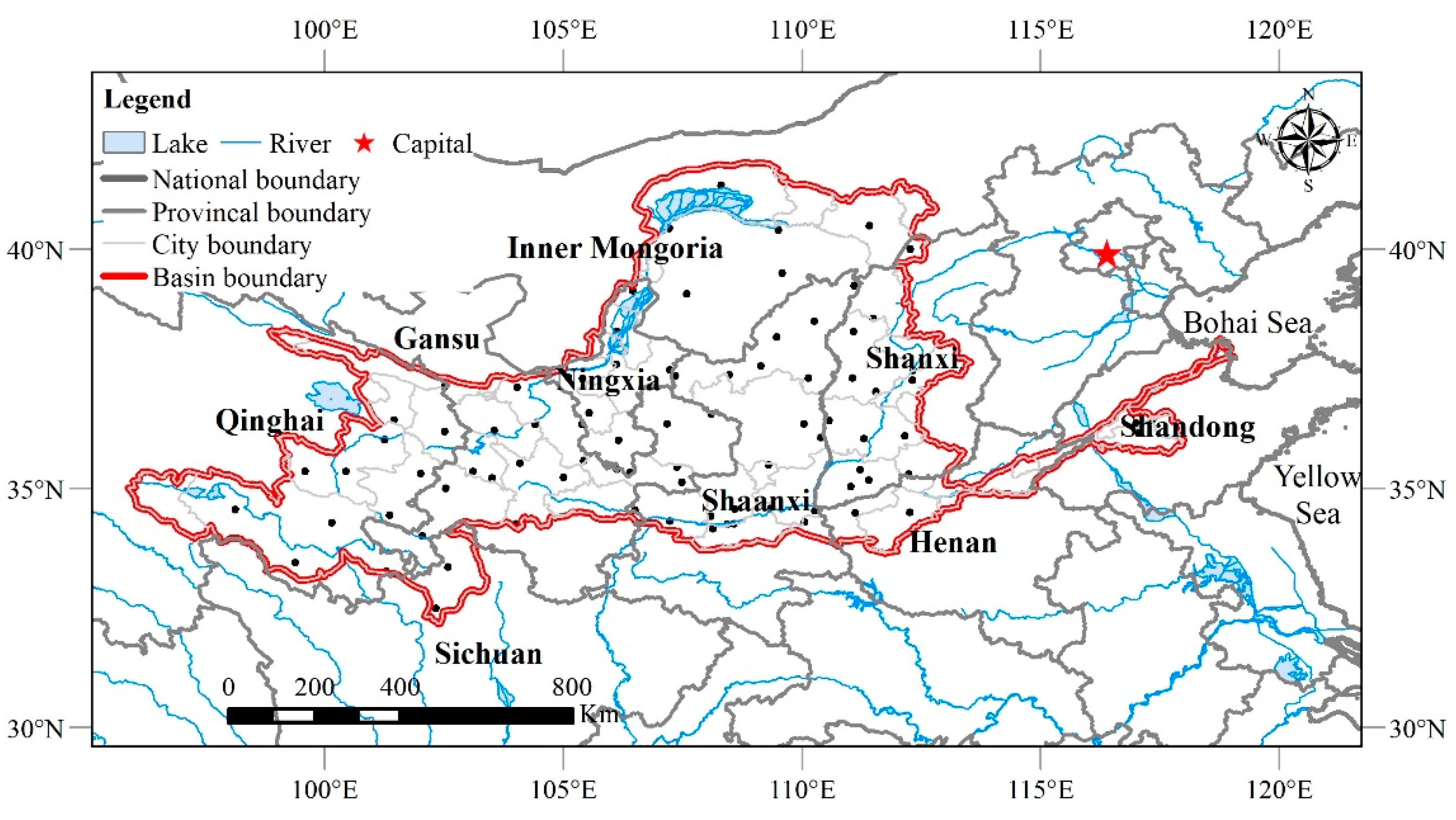
The Yellow River, which is the second longest river in China, originates from the Bayan Har Mountains. It flows through the nine provinces and regions of Qinghai, Sichuan, Gansu, Ningxia, Inner Mongolia, Shaanxi, Shanxi, Henan, and Shandong, and flows into the Bohai Sea. The Yellow River Basin is located at 95° E–120° E, 30° N–45° N, with an area of 794,000 km2 (Figure 1). The elevation of the basin gradually decreases from upstream to downstream. The upstream is mostly mountains and grassland plateau, the middle reaches are part of the Loess Plateau, and the downstream is the North China Plain. The basin is located in the middle latitude zone. The climate has strong regional differentiation and the annual and seasonal changes of various climate elements are large under the dual influence of atmospheric and monsoon circulation. The average annual precipitation distribution ranges from 130–1000 mm, and the precipitation decreases from southeast to northwest. About 70% of the precipitation is concentrated from June to September. The temperature ranges from −9 to 18 °C, and the east–west variation of temperature is greater than that in the north–south direction [33].
The Yellow River Basin spans 77 prefecture-level cities in nine provinces and regions of China, accounting for 8.6% of the total population of China. It is an important major grain producing area in China, with rich land and energy resources. It plays an important role in China’s economic and social development layout and is a region that must be guaranteed for China’s strategic development. The Yellow River Basin is one of the major grain producing areas in China. The cultivated land area accounts for 12.5% of the whole country, among which the Ningmeng Hetao Plain in the upper reaches, the Fenwei basin in the middle reaches, and the Yellow River irrigation area in the lower reaches are all main agricultural production bases. At the same time, the basin is rich in natural resources, including hydropower resources in the upper reaches, coal resources in the middle reaches, and oil and natural gas resources in the lower reaches, which occupy an extremely important position in the country. As China’s agricultural economic development area and energy basin, water for agriculture and energy industry account for 75% and 9% of the total water consumption of the Yellow River Basin, respectively. However, the water resources in the Yellow River Basin accounts for only 2.6% that of China, and the per capita amount of water resources is 620 m3, accounting for only 30% of the national average. It is one of the areas of China with the biggest shortage of water resources and has become the main bottleneck, restricting local development.
2.2. Dataset
The data of water resources, energy, and food required for this study are compiled from different sources. Water resource quantity and water use data by industry of prefecture level cities are extracted from the China Statistical Yearbook, China Water Conservancy Yearbook, China Water Conservancy Statistical Yearbook, Water Resources Bulletin of Yellow River Basin, Water Resources Bulletin in province, Statistical Yearbook in province, etc. The data period is 1998–2018. Individual missing data are interpolated in combination with the precipitation data of meteorological stations.
The meteorological daily data are collected from the China Meteorological Data Network (http://data.cma.cn (accessed on 13 May 2022).) for the period from 1998 to 2018 [34]. The annual precipitation of prefecture level cities is converted according to the Tyson polygon method and time scale.
The grain field and farmland area of prefecture level cities are extracted from the China Urban Statistical Yearbook, China Statistical Yearbook, and Statistical Yearbook in provinces. The data period is 1998–2018 on a prefecture-level city scale. Primary energy production comes from the China Statistical Yearbook and China Energy Statistical Yearbook. The data period is 1998–2018 on the provincial scale.
3. Methodology
3.1. Standard Deviation Ellipse and Resource Center of Gravity Transfer
The standard deviation ellipse is a classic algorithm used to analyze the direction and distribution of a group of data [35]. Three standard parameters are required, including the center, rotation angle, and length of major and minor axes in drawing the standard deviation ellipse. The center is the center of gravity of the resource element distribution. For a study area with n small areas, the center of gravity is calculated as follows:
where (xi, yi) refers to the central coordinate of the i-th small area, wij is the value of a spatial element in the t-th year of the i-th small area (also called the spatial weight of the area), Gt(xt, yt) is the center of gravity coordinate of the spatial element in the whole study area in the t-th year.
The rotation angle β is the angle of clockwise rotation in the due north direction to the long axis of the ellipse. The calculation formula is as follows:
where , are the coordinate deviation between the center of each small area and the center of gravity of the study area. Based on this, the standard deviation of the major axis () and the minor axis () can be calculated, respectively.
The resource center of gravity and standard deviation ellipse methods were used to characterize the distribution and evolution direction of watershed resources. The distance between the center of gravity of resources and the geometric center of the study area represents the balance of spatial distribution of resources. The farther the distance is, the more unbalanced the spatial distribution is. The deviation direction is the distribution concentration area. The moving direction and distance of the resource center of gravity indicate the direction and deviation intensity of the spatial resource redistribution, respectively. The standard deviation ellipse coverage represents the main area of the spatial distribution of features. In this paper, water resources, farmland area, and primary energy production are used to characterize the resource status of the WEF system in the Yellow River basin.
3.2. Lorentz Curve and Gini Coefficient
The Gini coefficient and resource matching coefficient can both be used to scientifically evaluate the degree of resource matching. The former can comprehensively evaluate the matching status of a whole region, while the latter can refine the spatial distribution of the cognitive matching pattern. The Gini coefficient method can be used to evaluate resource balance, which is usually calculated in combination with the Lorentz curve. We assume that curves M and N are absolute mean curve and Lorentz curves, respectively, and the Gini coefficient–called the Gini coefficient (called Gn for short), Gn∈ [0,1] is twice the area enclosed between curves M and N. The more that curve N deviates from M, the larger the area surrounded by the two, the greater the Gn, and the worse the matching degree of resources. The calculation formula is as follows:
When the Gini coefficient method is used to calculate the Gini coefficients of agricultural water–farmland and industrial water–energy in the basin, the specific calculation formula is as follows:
where Wi refers to the cumulative percentage of water resources on the i-th small area in the total regional water resources, Ri refers to the cumulative percentage of farmland area or primary energy production on the i-th small area in the total regional amount.
3.3. Resource Matching Coefficient Method
The agricultural water–farmland resources matching coefficient refers to the amount of agricultural available water resources per unit farmland area. The greater the value, the higher the matching degree. The calculation formula is as follows:
where Xi is the agricultural water–farmland resources matching coefficient of the i-th prefecture level city, wi, αi, βi are the total of water resources, the proportion of available agricultural water, and the farmland area in the i-th prefecture level city.
The industrial water–energy resource matching coefficient is defined as the amount of available industrial water resources per unit of energy production. The greater the value, the higher the matching degree. The calculation formula is the same as Formula (7). Xi, wi, αi, βi represent the agricultural water–farmland resources matching coefficient, the total water resources, the proportion of industrial available water, and the primary energy production in the i-th prefecture level city, respectively.
3.4. Multivariate Joint Probability Distribution Based on Copula Function
The Copula function is a multidimensional joint analysis method with a uniform distribution domain [0,1], which is widely used and expressed as follows.
Based on Copula’s two-dimensional (2-Copulas) and three-dimensional (3-Copulas) joint distribution model, the joint distribution of water resources, energy production, and grain production in the Yellow River Basin were constructed in this paper. The main steps are as follows.
- Step 1: Construction of marginal distribution.
Eight kinds of method are selected for edge distribution fitting, including Rayleigh distribution, Weibull distribution, Gamma distribution, Lognormal distribution, Normal distribution, Poisson distribution, Exponential distribution, and Extreme value distribution. The maximum likelihood estimation (ML estimation) is used to estimate the parameters of edge distribution, shown as Formulas (9) and (10).
where L(θ) refers to the likelihood function. Just make and is the maximum likelihood estimate value of parameter θ. Then, the marginal distribution line with the best fitting effect for the data series is determined by a goodness-of-fit test based on the Kolmogorov Smirnov test (K-S), mainly used for discrimination. The formula is as follows.
where D is the statistical variable of the K-S test, Ck is the theoretical frequency value of the measured samples, i is the serial number of the measured samples sorted in ascending order, and N is the number of samples. According to the significance level, check the table to obtain the critical test value , and accept the test when [36].
- Step 2: Fitting of 2-Copulas and 3-Copulas.
Five kinds of 2-Copulas and four kinds of 3-Copulas distribution functions are used for element fitting, as shown in Table 1. The maximum likelihood estimation method is also used for the parameter estimation of the Copula function. The root mean square error (RMSE) and Akaike Information Criterion (AIC) method are used for the goodness-of-fit test in order to determine the optimal copula function satisfying the parameter range.
where Pei is the joint empirical probability, Pi is the Copula value of the observation sample, and e is the number of parameters. The lower the value of RSME and AIC, the better the fitness performance.
4. Results
4.1. Resource Distribution and Transfer Direction of WEF
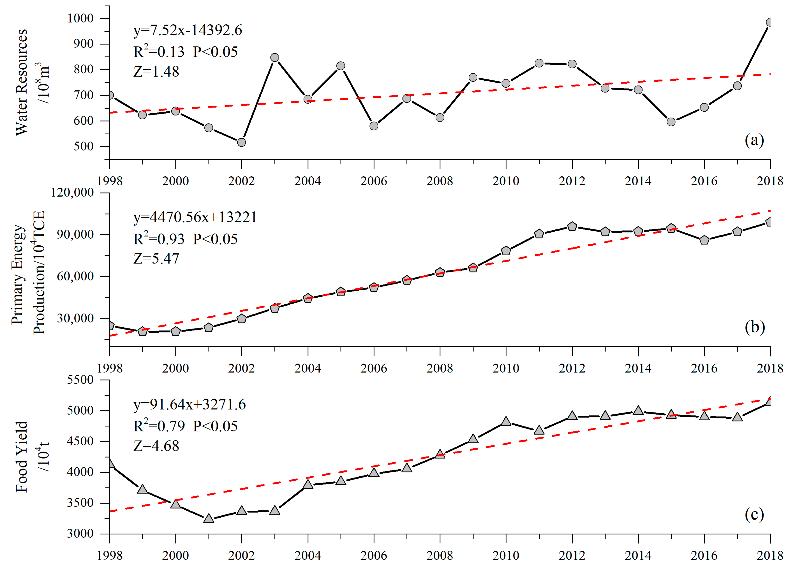
The variation of water resources, primary energy production, and total grain yield in the Yellow River Basin from 1998 to 2018 are shown in Figure 2. Over the past two decades, the average of annual water resources in the Yellow River Basin was 7.08 × 10¹⁰ m3, and the water resources have shown an insignificant increasing trend (|z| < 1.64, p < 0.05). Water resources were abundant in the Yellow River Basin before the 1970s, and then were at a relatively dry level due to the reduction in precipitation from 1970 to 2000. After the year 2000, water resources began to show an increasing trend. The mean primary energy production was about 6.24 × 10⁸ TCE (TCE is a unit of energy measurement, meaning ton of standard coal equivalent) and showed a significant increasing trend (|z| > 1.64, p < 0.05), especially in Shaanxi, Inner Mongolia, Shanxi, and other provinces in the middle reaches of the Yellow River Basin. As one of the largest energy bases in China, the energy production of the Yellow River Basin has been increasing with the increase of social demand and the development of industrial technology. The mean farmland area was about 1.25 × 10⁷ hm2, the cultivation area was about 1.04 × 10⁷ hm2, the average grain yield was about 4.23 × 10⁷ t, and the unit yield was about 4200 kg/hm2. Shanxi, Shaanxi, Shandong, Gansu, Henan, and other places are the main production areas. The total food yield in the Yellow River Basin showed a significant increasing trend (|z| > 1.64, p < 0.05). The evolution regular can be divided into two stages. As can be seen from Figure 2c, the food yield of the Yellow River Basin decreased significantly from 1998 to 2003. The agricultural production in the middle reaches was affected by the policy of returning farmland to forest and grassland, so the reduction of farmland area was the main reason for the reduction of food yield. From 2003 to 2018, food yield began to increase steadily, which is the result of the adjustment of agricultural planting structures and the continuous progress of production technology.
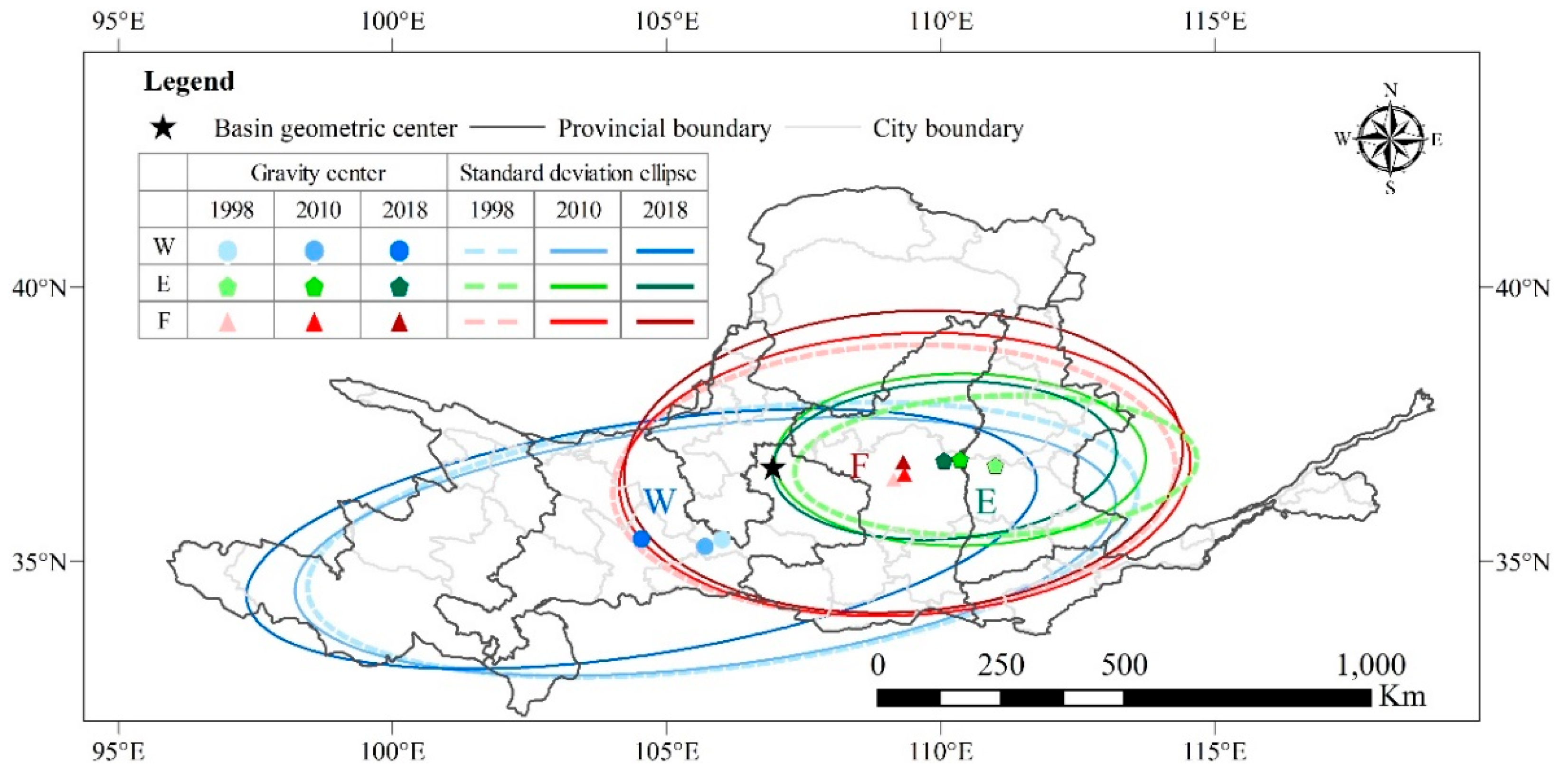
Water resources, primary energy production, and farmland area were used to characterize three representative resource indicators in water, energy, and food systems, respectively. The resource center of gravity and standard deviation ellipse method were used to indicate the main distribution range and resource transfer direction of the resources, and the results are shown in Figure 3. The circle (blue), pentagon (green), and triangle (red) in the figure respectively represent the resource center of gravity of the three resource indicators of WEF, and the color from light to dark represents the change of time. The color change of the standard deviation ellipse is the same as the indicated color of the resource center of gravity.
From the distribution range of the standard deviation ellipse, it can be seen that the areas rich in water resources, farmland, and energy in the Yellow River Basin are concentrated in the upper reaches, middle and upper reaches, and middle and lower reaches of the basin, respectively. Additionally, the concentrated distribution area of energy resources is relatively small. Furthermore, the centers of gravity of WEF resources all have a certain distance from the geometric center of the basin, which indicates that the distribution of resources were uneven in the area. From 1998 to 2010 and then to 2018, the transfer directions of water resources, energy production, and farmland area in the basin were not very consistent. The center of gravity of water resources, energy production, and farmland area were shifted to the northwest, northeast, and west of the basin, respectively. The transformation of the elliptic distribution range of standard deviation is consistent with the transfer direction of the center of gravity of resources. The transfer direction of water resources is opposite to that of farmland resources, and the degree of mismatch shows an intensifying trend. Although the transfer direction of water resources and energy resources is consistent, the matching degree is still not high. Generally speaking, the development of WEF in the Yellow River Basin is unbalanced and mismatched, and the difference in the evolution of resources in time and space intensifies this phenomenon [37].
4.2. Temporal Variation of Resource Balance Level in WEF Systems of the Yellow River Basin
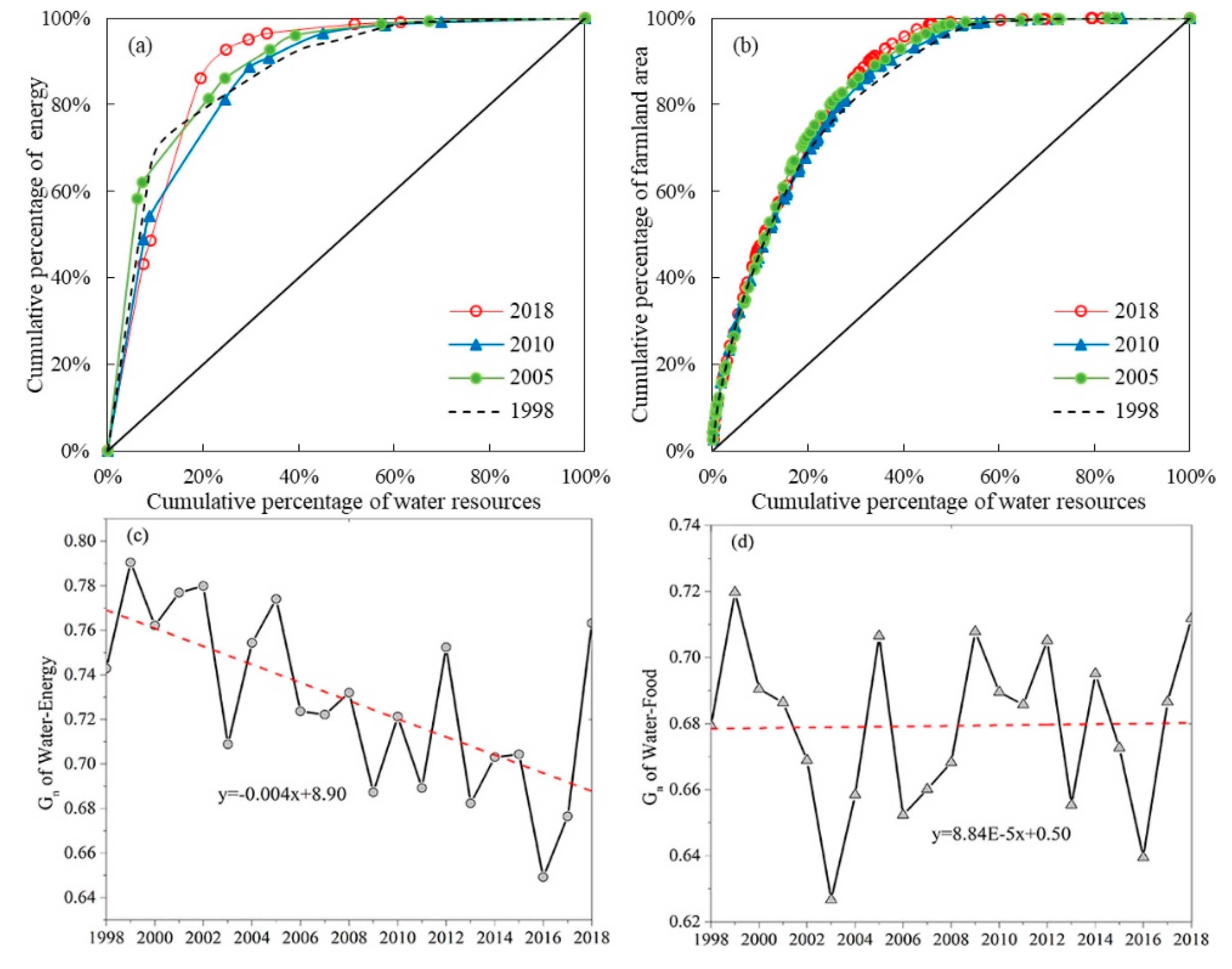
The Gini coefficient method was used to calculate the resource balance of agricultural water–farmland and industrial water–energy in the whole basin. The Lorentz curve and calculation results are shown in Figure 4. According to the definition and calculation principle of the Gini coefficient, the greater the Gini coefficient, the worse the balance of resource development. For the balance condition between industrial water resources and energy, the annual average Gini coefficient of the Yellow River Basin is about 0.728, and shows a decreasing trend. The industrial Gini coefficient fluctuated from 1998 to 2016 and reached its lowest value of 0.65 in 2016, indicating that the matching of water and energy resources in the basin tends to improve, and the gap between different prefecture level cities is narrowed. From 2016 to 2018, the Gini coefficient increased again, which shows that there are still some risks in the coordinated development of industrial water and energy in the Yellow River Basin.
For the balance condition between agricultural water resources and farmland, the average Gini coefficient of the Yellow River Basin is about 0.688, showing an increasing trend from 1998 to 2018, which means that the matching degree of water and land resources in the basin tends to deteriorate and become more unbalanced. During different periods, the Gini coefficient decreased year by year from 1998 to 2003, reaching the lowest value of 0.62 in 2003. Meanwhile, the Gini coefficient began to fluctuate and increase from 2003 to 2018; this indicated that the agricultural water and land resources in the Yellow River Basin are increasingly mismatched and the regional development is uneven. It is more difficult for water resources to meet cultivated land.
4.3. Spatial Matching Pattern in Industrial Water–Energy and Agricultural Water–Farmland Resources
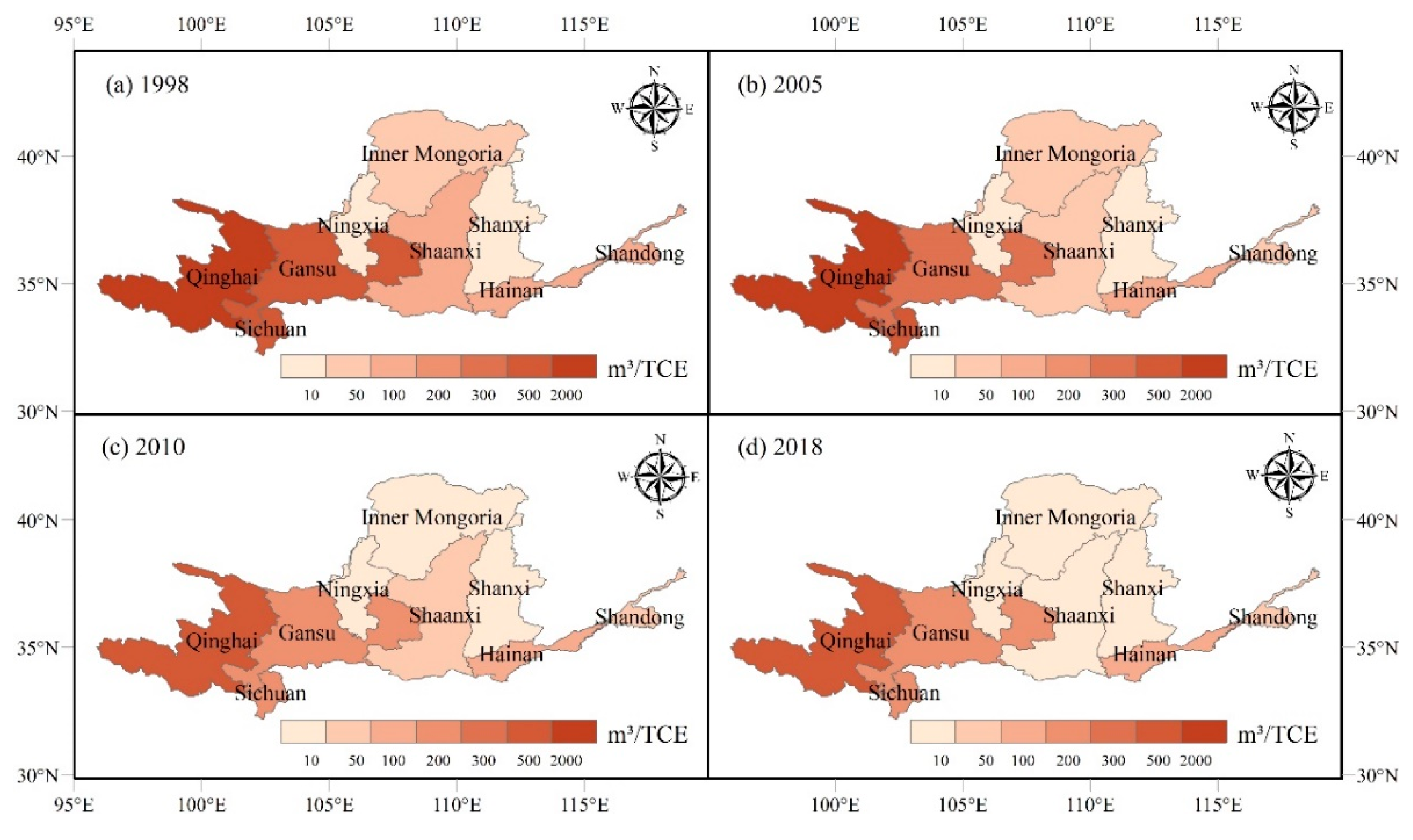
Based on the understanding of the matching degree of the basin in general, the resource matching coefficient method was used to refine and analyze the machine evolution characteristics of the spatial matching pattern of resources. The calculation of the industrial water–energy matching pattern is shown in Figure 5. The spatial matching coefficient in the upper reaches of the Yellow River Basin is relatively large, while the matching coefficient in the middle and lower reaches of the Yellow River Basin is relatively low. According to the calculation formula of the matching coefficient, the greater the matching coefficient, the better the matching degree of resources in this area. The upstream area is relatively rich in water resources, while the energy production is low. The amount of water resources more easily meets the needs of energy development, so the matching degree is better. However, in Shanxi, Shaanxi, Inner Mongolia, and other places of the middle reaches, the abundance of energy resources is high with a relative shortage of water resources. It is difficult for water resources to meet the demand of energy production, so the matching degree is poor. The water energy matching coefficient of all provinces in the basin tends to decrease, and the water–energy matching degree decreases. This is because it is difficult for the change of water resources to meet the demand of high-speed energy production, which is not conducive to sound development.
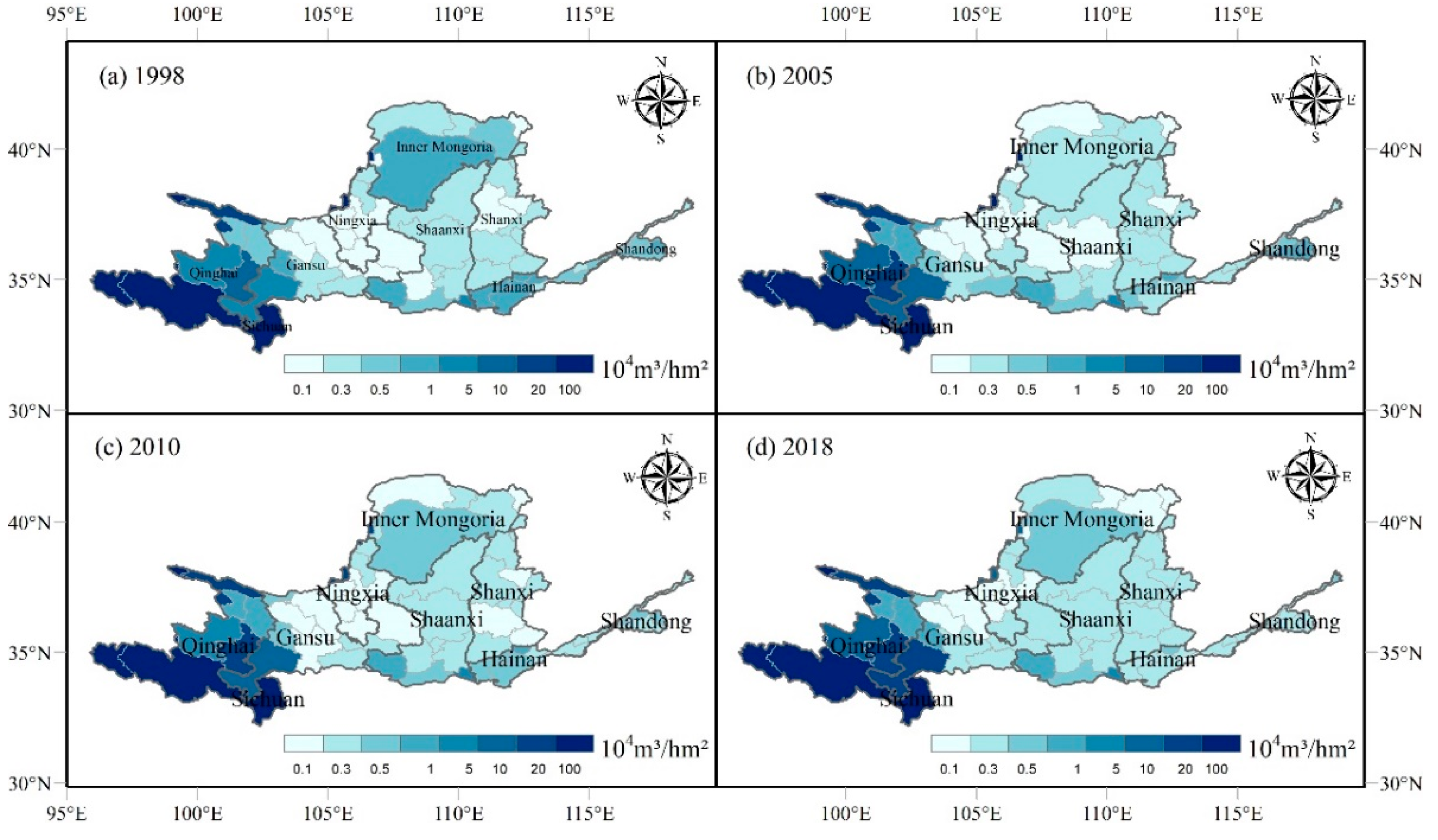
The agricultural water–farmland matching pattern is shown in Figure 6. It can be seen that in the source area of the Yellow River with abundant water resources and less farmland, the matching coefficient is the largest. The agricultural matching degree in the source area is the highest. The matching coefficient of other areas in the basin is relatively small and the matching condition is poor, because the farmland is concentrated in these areas and the distribution of water resources is not extensive enough to fully meet the demand for agricultural water. In certain cities in the Ningxia Hui Autonomous Region and Gansu Province, the matching degree is the lowest, which is due to the lack of regional precipitation and water resources. The matching degrees of Shanxi, Shaanxi, and other places take second place, which is also related to the disharmony of water resources and farmland area. In addition to the deterioration of the matching degree between the Ningmeng Irrigation Area (Ningxia and Inner Mongoria) and the downstream area, which is caused by the increase in the farmland area and the decrease in agricultural water consumption, the matching degree of the basin in most areas of the source area and the middle reaches is improving. These areas need to be focused on in the future.
4.4. Nexus of WEF System
Eight kinds of common methods are selected for edge distribution fitting in this paper. At a significance level α = 0.05 ( = 0.296), it is confirmed that the water resources, primary energy production, and grain yield in the Yellow River Basin fit to Weibull distribution, lognormal distribution, and Weibull distribution, respectively. Then, the Copula functions are used to evaluate the nexus of the WEF system. The two-dimensional copula (2-Copulas) function is used to fit the two-dimensional joint distribution between water resources and primary energy production (W–E), water resources and grain yield (W–F), and primary energy production and grain yield (E–F), respectively. Five kinds of 2-Copulas functions were selected for two-dimensional distribution fitting. The ML estimation method is used to calculate the parameters, and the optimal fitting function is selected based on the minimum RMSE and AIC by calculation of the theoretical frequency and empirical frequency. The results are shown as Table 2. Therefore, Clayton Copula (AIC = −340.04, RSME = 0.017), Clayton Copula (AIC = −292.12, RSME = 0.03), and Frank Copula (AIC = −350.66, RSME = 0.015) were selected to fit the Copula function of W–E, W–F, and E–F in this paper. The formula of the two-dimensional Copula distribution function can be obtained by substituting the parameters into the formula in Table 1.
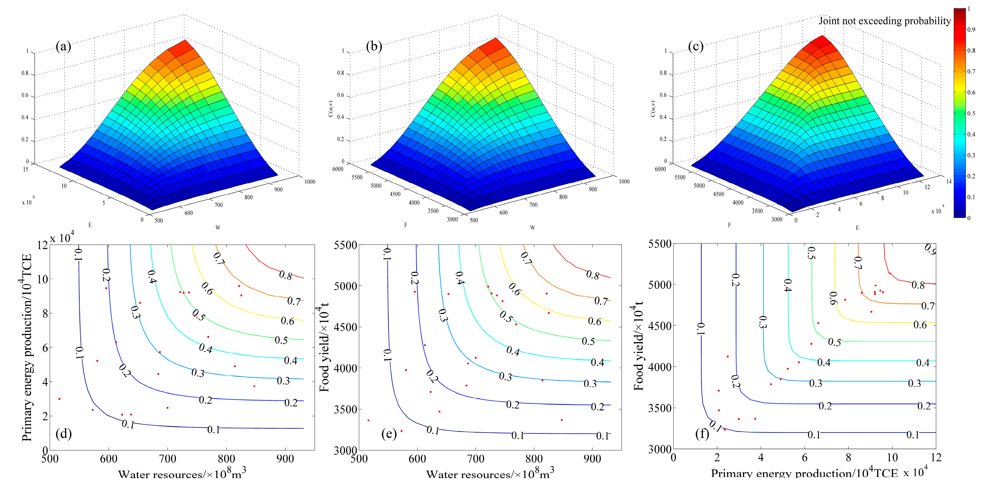
The joint distribution C (u, v) and section contour map of W–E, W–F, and E–F in the Yellow River Basin from 1998 to 2018 was shown as Figure 7. For example, C (u, v) is defined as the joint distribution probability (also called joint not exceeding probability) when W ≤ u, E ≤ v occur at the same time in W–E, which is similarly with W–F and E–F. It can be seen that the joint probability shows an increasing trend when the variables are large at the same time. As shown in Figure 7d, when the water resources are constant, the greater the primary energy production, or when the energy production is constant, the greater the water resources, the greater the joint distribution probability. The mean value of water resources, primary energy production and food yield are 7.08 × 10¹⁰ m3, 6.24 × 10⁸ TCE, 4.23×10⁷ t, respectively. As shown in Figure 7d–f), the joint probability of W–E measured value (W ≤ 7.08 × 10¹⁰, E ≤ 6.24 × 10⁸) is about 0.35, and there are 8 years of data within this probability range. The joint probability of W–F measured value (W ≤ 7.08 × 10¹⁰, F ≤ 4.23 × 10⁷) is about 0.32, and there are 9 years of data within this probability range. The joint probability of E–F measured value (E ≤ 6.24 × 10⁸, F ≤ 4.23 × 10⁷) is about 0.43, and there are 10 years of data within this probability range. Moreover, they are all concentrated in 1998–2008.
Then three kinds of copula function were used to fit the three-dimensional joint distribution (3-Copulas) of water resources, primary energy production and grain yield, including Gaussian Copula, t Copula and Gumbel-Hougaard Copula. The parameters and results are shown in Table 3. Therefore, t Copula (AIC = −286.29, RMSE = 0.03) is determined as the best fit copula function. The distribution function of three-dimensional t Copula function can be obtained according to the parameters.
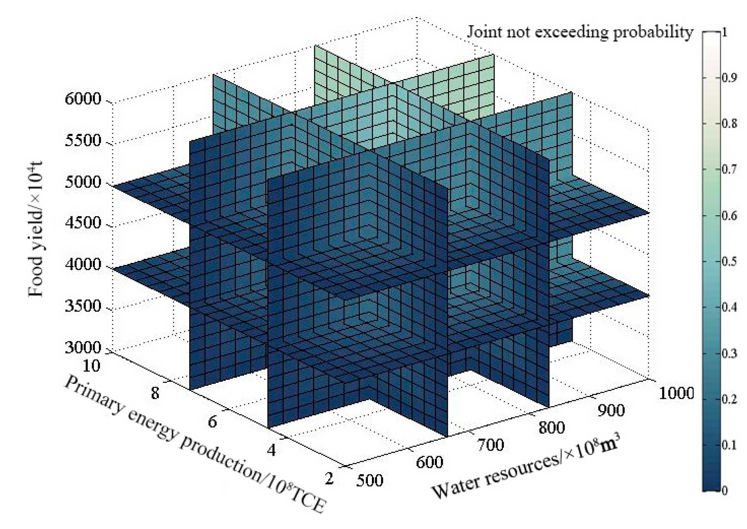
From the analysis above, it can be seen that the three-dimensional t Copula function can be applied to the study of three-dimensional joint distribution C (u, v, w) of WEF system in the Yellow River Basin. The three-dimensional joint probability diagram of W–E–F is shown as Figure 8. C (u, v, w) represents the joint distribution probability of W ≤ u, E ≤ u, F ≤ w occurring at the same time. When the conditions of two variables are certain, the three-dimensional joint probability increases with the increase of the other variable. When the three characteristic variables all increase, the cumulative probability finally approaches 1. The joint distribution probability of W–E–F (W ≤ 7.08 × 10¹⁰, E ≤ 6.24 × 10⁸, F ≤ 4.23 × 10⁷) is about 0.3–0.4. The measured value of W–E–F in 8 years is within this probability range, which is also concentrated in 1998–2007. After that, water resources, primary energy production, and grain yield all increased from 2008 to 2018. In the future, the W–E–F system will tend to increase and expand in the Yellow River Basin. In particular, there should be more attention paid to whether the water resources can meet the needs of industrial and agricultural development. It is necessary to coordinate the relationship between water–energy, water–food, and food–energy.
As a highly complex correlation system, it is difficult to describe the correlation characteristics of the WEF systems by single variable. There are certain advantages to analyzing the internal correlation or nexus relationship by establishing the multivariable joint distribution analysis system based on the Copula function. The Copula function is essentially an expression of joint distribution, which can describe or calculate the correlation among variables. The Pearson correlation coefficient and Rank correlation coefficient are the common methods used to describe correlation, however, the former can only reflect the linear correlation between variables, while the latter is more suitable for hierarchical variables [38]. In most cases, especially in complex system problems, the nexus correlation among variables is very complex, and changes with the change of variable value. These correlation coefficients are global, and thus cannot provide details of the change of correlation among variables. In addition, these coefficients only provide numerical values and indicating nothing about the specific structure and function of the nexus of the system. The Copula function can provide the structure and function details related to variables in different value ranges. The Copula joint distribution constructed in this paper can pass the K-S, AIC, and RMSE statistical value test, which shows that it can adequately describe the nexus of the WEF system in the Yellow River Basin.
5. Discussion
5.1. Comparison of the WEF Matching Pattern among the Yellow River Basin and Other Regions
In order to reflect the matching status and level of water–energy–food in the Yellow River Basin more intuitively, some relevant data are collected to compare the matching degree of the WEF system in different regions. The resource matching Gini coefficient was compared throughout the Yellow River Basin and other regions, as shown in Table 4. As mentioned above, the greater the Gini coefficient (closer to 1), the more unbalanced the development of resources. For the development balance between industrial water resources and energy, the Gini coefficient of water–energy matching in the Yellow River Basin is 0.728, and China’s national average Gini coefficient ranges 0.85–0.89 [39], indicating that the water–energy matching degree in the Yellow River Basin is better than the national average. However, the warning threshold for the Gini coefficient of water–energy matching in the world is only about 0.4 [40], and the value of the Yellow River Basin is far greater than the world warning threshold. In other words, although the water–energy matching in the Yellow River Basin is relatively better than that in China, it is far inferior to the international warning level.
For the resource development balance between agricultural water resources and farmland, the Gini coefficient of water–land matching is 0.688 in the Yellow River Basin. The Gini coefficient of the world, Asia, and China is 0.586, 0.550, and 0.566, respectively, which is relatively close [41,42]. It can be seen from the values that the order of Gini coefficient from small to large is Asia, China, the world, and the Yellow River Basin. That is, the matching degree of China’s water–land resources is better than the world average, but lower than the Asian average. Additionally, the matching degree of the Yellow River is relatively worst. However, the current Gini coefficient (0.566) is less than the background Gini coefficient (0.712) at the Chinese level [43]. The current Gini coefficient refers to the amount of water resources per unit of actual cultivated land area, while the background Gini coefficient refers to the amount of water resources per unit of potential cultivated land area. It also shows that although the matching degree of water and farmland in the Yellow River Basin is poor at the Chinese level, it has been improved under the action of artificial adjustments and controls, and measures still need to be taken for macro-control in the future.
5.2. Discussion on Security Risk and Adaptive Development Strategy of the WEF System
Understanding the relationship and the evolution law of the matching pattern among the resource elements is the foundation to ensuring the security of the regional WEF system. Many scholars have evaluated the comprehensive system security or system risk in different regions through different index evaluation systems [26,44]. For example, Wang et al. evaluated the security of China’s water–energy–food system by improving the matter–element expansion model [45]. Li evaluated the security of China’s WEF system from the perspectives of stability, coordination, and sustainability by using the synergetic symbiosis theory [22]. The results show that the safety of China’s WEF system is at a certain risk level and may deteriorate in the future. Mohammadpour et al. quantitatively evaluated the security of the water–energy–food system in three South American countries based on the Rand-Pardee system evaluation method [46]. In addition, the coupling coordination model [47,48], cloud matter element model [49], and other evaluation methods have also been applied. It is very important to identify the key factors affecting the system security based on the evaluation of the WEF system security [50,51], which is helpful to formulate scientific and reasonable control strategies or future measures for relevant decision-making departments. However, the influencing factors of the WEF system security in different regions are different in different periods [52]. There are many key factors threatening the security of the WEF system, such as population growth, shortage of water resources, frequent extreme events and natural disasters, economic and social development, and so on [53,54]. The population growth leads to a sharp increase in food demand, an increasing demand for energy by economic and social development, and an uneven temporal and spatial distribution of water resources caused by natural changes, which will all increase the security risk of the WEF system. For China, the main factors putting pressure on the WEF system include population density, dietary structure change, and economic development, which will be paid special attention in the future [55,56].
The WEF system is vulnerable to external driving factors. In addition to natural factors related to climate and the environment, man-made control policies related to economic and social development and ecological environment protection will also affect the WEF system [57]. Therefore, policies and measures simultaneously need to be considered based on the evaluation of the WEF system relationship [58]. The Yellow River Basin is a typical area in China with prominent water–energy–food contradictions. Water resource constraints increase the risks of energy security, food production vulnerability, and ecological environment vulnerability [47]. In the future, decision-making departments need to improve the existing policies or put forward newer and more powerful measures to ensure the safety and sustainable development of the WEF in the Yellow River Basin based on the understanding of WEF relationships. Different measures need to be taken in terms of water resources, energy, and food in different areas to improve the collaborative security level of the WEF system. For example, in terms of water resources, we should strictly control the total amount of water used, promote the optimization of water use structure, save water efficiently, and control water. In terms of energy, we should promote the transformation of water consumption industries to water intensive and economical utilization industries, adjust energy consumption structures, and increase the proportion of clean energy. In terms of food production, we should optimize crops and adjust planting structures, improve the efficiency of irrigation and water use, improve water-saving and field management technology, and plan water transmission and distribution schemes reasonably. In addition, reducing food waste in logistics, warehousing, transportation, consumption, and other links is also an important measure to reduce food risks. In addition, it is necessary to further deepen regional cooperation, adjust measures to local conditions, support each other, and share the pressure. It should be noted that the plannings or policies should strengthen the overall consideration of multi resources and the nexus of water, energy, and food [59]. There should be more attention paid to the integrity of the system, developing multiple types of policies at the same time to avoid disconnection in a certain field.
5.3. Uncertainty Analysis and Limitations
Due to the uneven distribution of natural resources, the aggregation of population distribution, and the imbalance of economic development in the Yellow River Basin, the problems of WEF spatial pattern mismatch and uneven development may exist for a long time. In this paper, the temporal and spatial matching pattern and resource evolution law of water, energy, and food are evaluated, and the nexus of the WEF system is established and analyzed. However, the cross-department, multi-caliber, and multi-scale characteristic of the WEF system and the fuzziness of the system boundary increase the difficulty of data acquisition and integration [60,61]. Considering the relative integrity of the data, the inter provincial scale and prefecture level city scale are used to evaluate the industrial water–energy production and agricultural water–farmland, with water as the link. Although it can reflect the distribution and evolution of resource elements of the WEF system, it can further improve the spatial accuracy in the future. Furthermore, the influence of external factors (economy, society, and environment) on the system is not considered when establishing the multi-dimensional joint distribution to analyze the nexus of the WEF system in this paper. In the future, we can continue to further analyze the dynamic feedback control simulation and response of WEF systems to the changes of external factors.
6. Conclusions
As an important food and energy production base, the Yellow River Basin is selected as the study area of this paper, in which the shortage of water resources has caused the increasingly serious contradiction among the development of water, energy, and food resources. The spatiotemporal matching pattern and nexus of the WEF system elements were evaluated and analyzed from a 1-dimensional, 2-dimensional, and 3-dimensional perspective, respectively. The standard deviation ellipse and resource gravity center methods were used to describe the distribution and transfer direction of resources in the Water–Energy–Food system. The Gini coefficient and resource matching coefficient method were applied to evaluate the matching pattern and variation of agricultural water-farmland and industrial water–energy production. Multivariate joint probability distribution was established to evaluate the nexus of the WEF system. The main conclusions are as follows:
- (1)
- The areas rich in water resources, farmland, and energy in the Yellow River Basin are not consistent; they are concentrated in the upper reaches, middle and upper reaches, and middle and lower reaches, respectively. In addition, the transfer directions were shifted to the northwest, northeast, and west, respectively. That is, the distribution of water resources, farmland, and energy are uneven themselves, and the evolution directions are also different.
- (2)
- The annual average Gini coefficient of industrial water–energy is about 0.728, showing a decreasing trend, which demonstrates that the gap has reduced in sub-region recent years. The average Gini coefficient of agricultural water–farmland is about 0.688, showing an increasing trend, which means the gap in different sub-regions has widened slightly.
- (3)
- Spatially, the matching degree of water and energy in the upper reaches is good, while that in the middle reaches is poor. The matching degree of each province is reduced. For the matching between water and farmland, the source area of the Yellow River has abundant water resources and less farmland, resulting in the highest matching degree. In addition to the poor matching degree between the Ningmeng Irrigation Area and the downstream, the matching degree in most areas of the source area and the middle reaches is improving.
- (4)
- Eight kinds of marginal distribution, five kinds of 2-Copulas, and three kinds of 3-Copulas were used to establish the joint distribution in order to simulate the nexus of the WEF system in the Yellow River Basin. The t Copula function can describe the nexus of the WEF system in the Yellow River Basin tested by statistical methods. The correlation and nexus among the system variables are described in detail through the joint distribution function, which can reflect the specific structure and function of the nexus in the WEF system.
The problems of spatial pattern mismatch and uneven development may exist in the WEF system of the Yellow River Basin for a long time. In future research, the feedback effect inside the system and the impact of external stress factors on the system can continue to be explored on the basis of more detailed data.
Author Contributions
This study was calculated and written by J.W.; Z.B. and J.Z. designed the experimental framework of this work; G.W. and C.L. provided the calculation method; H.W. and Y.Y. contributed to the revision of manuscript and data collection. All authors have read and agreed to the published version of the manuscript.
Funding
This research is funded by several research programs: (1) The National Key R&D Program of China (grant No.2017YFA0605002); (2) The National Natural Science Foundation of China (grant No. 41961124007, 51879164); (3) “Six top talents” in Jiangsu province (grant No. RJFW-031).
Institutional Review Board Statement
Not applicable.
Informed Consent Statement
Not applicable.
Data Availability Statement
The data presented in this study are available on request from the corresponding author or the first author.
Conflicts of Interest
The authors declare no conflict of interest.
References
- Rasul, G.; Sharma, B. The nexus approach to water–energy–food security: An option for adaptation to climate change. Clim. Chang. 2016, 16, 682–702. [Google Scholar] [CrossRef] [Green Version]
- IPCC. Climate Change 2022: Impacts, Adaptation and Vulnerability; IPCC: Geneva, Switzerland, 2022. [Google Scholar]
- UNESCO. World Water Development Report 2020 ‘Water and Climate Change’; UNESCO: Paris, France, 2020. [Google Scholar]
- International Energy Agency. 2021 World Oil Outlook 2045; International Energy Agency: Paris, France, 2021. [Google Scholar]
- FAO. The State of the World’s Land and Water Resources for Food and Agriculture: Systems at Breaking Point (SOLAW 2021); FAO: Rome, Italy, 2021. [Google Scholar]
- Bazilian, M.; Rogner, H.; Howells, M.; Hermann, S.; Arent, D.; Gielen, D.; Steduto, P.; Mueller, A.; Komor, P.; Tol, L.; et al. Considering the energy, water and food nexus: Towards an integrated modelling approach. Energy Policy 2011, 39, 7896–7906. [Google Scholar] [CrossRef]
- Terrapon, P.J.; Ortiz, W.; Dienst, C.; Grone, M. Energising the WEF nexus to enhance sustainable development at local level. J. Environ. Manag. 2018, 223, 409–416. [Google Scholar] [CrossRef] [PubMed]
- Miguez, F.; Maughan, M.; Bollero, G.; Long, S. Modeling spatial and dynamic variation in growth, yield, and yield stability of the bioenergy crops Miscanthus x giganteus and Panicum virgatum across the conterminous United States. Gcb Bioenergy 2012, 4, 509–520. [Google Scholar] [CrossRef]
- Rigby, D.; Woodhouse, P.; Young, T.; Burton, M. Constructing a farm level indicator of sustainable agricultural practice. Ecol. Econ. 2001, 39, 463–478. [Google Scholar] [CrossRef]
- Forouzani, M.; Karami, E. Agricultural water poverty index and sustainability. Agron. Sustain. Dev. 2011, 31, 415–431. [Google Scholar] [CrossRef] [Green Version]
- Villholth, K.; Sharma, B.R. Creating synergy between groundwater research and management in South and SOUTHEAST ASIA. Proc. IWMI 2006, 39, 489–491. [Google Scholar] [CrossRef] [Green Version]
- Hoff, H. Understanding the Nexus; Background Paper for the Bonn 2011 Conference: The Water, Energy and Food Security Nexus; Stockholm Environment Institute (SEI): Stockholm, Sweden, 2011. [Google Scholar] [CrossRef]
- Bank, A.D. Thinking About Water Differently: Managing the Water-Food-Energy Nexus. Adb Rep. 2013, 1, 125184. [Google Scholar]
- FAO. The Water-Energy-Food Nexus: A New Approach in Support of Food Security and Sustainable Agriculture; FAO: Rome, Italy, 2014. [Google Scholar]
- Siebert, S.; Burke, J.; Faures, J.M.; Frenken, K. Groundwater use for irrigation—A global inventory. Hydrol. Earth Syst. Sci. 2010, 14, 1863–1880. [Google Scholar] [CrossRef] [Green Version]
- Corrales, J.; Naja, G.; Bhat, M.; Wilhelm, F. Modelling a phosphorus credit trading program in an agricultural watershed. J. Environ. Manag. 2014, 143, 162–172. [Google Scholar] [CrossRef]
- Hoekstra, A.Y.; Hung, P.Q. Globalization of water resources: International virtual water flows in relation to crop trade. Glob. Environ. Chang. 2005, 15, 45–56. [Google Scholar] [CrossRef]
- Wang, W.; Lv, N.J.; Wang, X.; Gao, C. Study on spatial matching pattern of water and soil resources in Yellow River delta. J. Water Resour. Water Eng. 2014, 25, 66–70. (In Chinese) [Google Scholar]
- Chao, Z.; Zhong, L.; Wang, J. Decoupling between water use and thermoelectric power generation growth in China. Nat. Energy 2018, 3, 792–799. [Google Scholar] [CrossRef]
- Soliev, I.; Wegerich, K.; Kazbekov, J. The costs of benefit sharing: Historical and institutional analysis of shared water development in the Ferghana Valley, the Syr Darya Basin. Water 2015, 7, 2728–2752. [Google Scholar] [CrossRef] [Green Version]
- Dargin, J.; Daher, B.; Mohtar, R.H. Complexity versus simplicity in water energy food nexus (WEF) assessment tools. Sci. Total Environ. 2018, 650, 1566–1575. [Google Scholar] [CrossRef]
- Li, X.; Liu, C.S.; Wang, G.Q.; Bao, Z.; Diao, Y.; Liu, J. Evaluating the collaborative security of Water–Energy–Food in China on the basis of symbiotic system theory. Water 2021, 13, 1112. [Google Scholar] [CrossRef]
- Deng, C.; Wang, H.; Gong, S.; Zhang, J.; Yang, B.; Zhao, Z. Effects of urbanization on food-energy-water systems in mega-urban regions: A case study of the Bohai MUR, China. Environ. Res. Lett. 2020, 15, 044140. [Google Scholar] [CrossRef]
- Li, G.J.; Li, Y.L.; Jia, X.J.; Lei, D.; Daohan, H. Establishment and simulation study of system dynamic model on sustainable development of water-energy-food nexus in Beijing. Manag. Rev. 2016, 28, 11–26. (In Chinese) [Google Scholar]
- Hussien, W.A.; Memon, F.A.; Savic, D.A. An integrated model to evaluate water-energy-food nexus at a household scale. Environ. Model. Softw. 2017, 93, 366–380. [Google Scholar] [CrossRef] [Green Version]
- Daher, B.T.; Mohtar, R.H. Water-energy-food (WEF) Nexus Tool 2.0: Guiding integrative resource planning and decision-making. Water Int. 2015, 40, 748–771. [Google Scholar] [CrossRef]
- Kraucunas, I.; Clarke, L.; Dirke, L.; Hathaway, J.; Hejazi, M.; Hibbard, K.; Huang, M.; Jin, C.; Kintner-Meyer, M.; van Dam, K.; et al. Investigating the nexus of climate, energy, water, and land at decision-relevant scales: The Platform for Regional Integrated Modeling and Analysis (PRIMA). Clim. Chang. 2015, 129, 573–588. [Google Scholar] [CrossRef]
- Kao, S.C.; Rao, S.G. Trivariate statistical analysis of extreme rainfall events via the Plackett family of copulas. Water Resour. Res. 2008, 44, 333–341. [Google Scholar] [CrossRef]
- Xie, H.; Luo, Q.; Huang, J.S. Synchronous asynchronous encounter analysis of multiple hydrologic regions based on 3 D copula function. Adv. Water Sci. 2012, 23, 186–193. (In Chinese) [Google Scholar]
- Zhang, X.; Ran, J.X.; Xia, J.; Song, Y. Jointed distribution function of water quality and water quantity based on Copula. J. Hydraul. Eng. 2011, 42, 483–489. (In Chinese) [Google Scholar]
- Zhang, Y.; Wang, K.; Liu, X.M.; Suchen, Z.; Jia, Z.; Cailin, W. The Three-dimensional Joint Distributions of Rainstorm Factors Based on Copula Function: A Case in Kuandian County, Liaoning Province. Sci. Geogr. Sin. 2017, 37, 603–610. (In Chinese) [Google Scholar]
- Li, H.F.; Wang, H.X.; Zhao, R.X.; Yang, Y. Estimating the symbiosis risk probability of water–energy–food using Copula function. Trans. Chin. Soc. Agric. Eng. 2021, 37, 332–340. (In Chinese) [Google Scholar]
- Yuan, M.; Wang, L.; Lin, A.; Liu, Z.; Li, Q.; Qu, S. Vegetation green up under the influence of daily minimum temperature and urbanization in the Yellow River Basin, China. Ecol. Indic. 2020, 108, 105760. [Google Scholar] [CrossRef]
- China Surface Meteorological Daily Data Set V3.0. Available online: http://data.cma.cn (accessed on 10 May 2020).
- Lefever, D.W. Measuring geographic concentration by means of the standard deviational ellipse. AJS 1926, 1, 88–94. [Google Scholar] [CrossRef]
- Massey, F.J. The Kolmogorov-Smirnov Test for Goodness of Fit. J. Am. Stat. Assoc. 1951, 46, 68–78. [Google Scholar] [CrossRef]
- Wang, J.H.; He, G.H.; He, F.; Yang, Z.; Haiye, W.; Haihong, H.; Youngnan, Z.; Hanquing, L. Utilization and matching patterns of water and land resources in China. South-North Water Transf. Water Sci. Technol. 2019, 17, 1–8. (In Chinese) [Google Scholar]
- Nelsen, R.B. An Introduction to Copulas; Springer Science: Berlin/Heidelberg, Germany, 2006. [Google Scholar]
- Liu, H.; Jia, Y.W.; Niu, C.W. Analyses of spatial distribution characteristic and matching pattern of regional water-energy resources. Water Resour. Power 2017, 35, 127–131+158. (In Chinese) [Google Scholar]
- Xiao, W.H.; Qin, D.Y.; Li, W.; Chu, J. Model for distribution of water pollutants in a lake basin based on environmental Gini coefficient. Acta Sci. Circumstantiae 2009, 29, 1765–1771. (In Chinese) [Google Scholar]
- World Resources Institute. World Resources Report; China Environmental Science Press: Beijing, China, 1999. [Google Scholar]
- Wu, Y.Z.; Bao, H.J. Regional Gini coefficient and its uses in analyzing to balance between water and soil. J. Soil Water Conserv. 2003, 17, 123–125. (In Chinese) [Google Scholar]
- Sun, Z.; Jia, S.F.; Yan, J.B.; Zhu, W.; Liang, Y. Study on the matching pattern of water and potential arable land resources in China. J. Nat. Resour. 2018, 33, 2057–2066. (In Chinese) [Google Scholar]
- Elias, M.H.; Matthew, L.; Aidong, Y. Understanding water-energy-food and ecosystem interactions using the nexus simulation tool NexSym. Appl. Energy 2017, 206, 1009–1021. [Google Scholar] [CrossRef]
- Wang, Q.; Li, S.; He, G.; Wang, X. Evaluating sustainability of water-energy-food (WEF) nexus using an improved matter-element extension model:a case study of China. J. Clean. Prod. 2018, 202, 1097–1106. [Google Scholar] [CrossRef]
- Mohammadpour, P.; Mahjabin, T.; Fernandez, J.; Grady, C. From national indices to regional action-An Analysis of food, energy, water security in Ecuador, Bolivia, and Peru. Environ. Sci. Policy 2019, 101, 291–301. [Google Scholar] [CrossRef]
- Peng, J.J. Coupling Relationship and Spatial-Temporal Differentiation of the Water-Energy-Food Nexus in the Yellow River Basin. Reg. Econ. Rev. 2022, 2, 51–59. (In Chinese) [Google Scholar]
- Sun, C.Z.; Yan, X.D. Security evaluation and spatial correlation pattern analysis of water resources-energy-food nexus coupling system in China. Water Resour. Prot. 2018, 34, 1–8. (In Chinese) [Google Scholar]
- Chen, J.; Yu, X.; Qiu, L.; Deng, M. Study on vulnerability and coordination of Water-Energy-Food system in northwest China. Sustainability 2018, 10, 3712. [Google Scholar] [CrossRef] [Green Version]
- Wicaksono, A.; Jeong, G.; Kang, D. Water, energy, and food nexus: Review of global implementation and simulation model development. Water Policy 2017, 19, 440–462. [Google Scholar] [CrossRef] [Green Version]
- Mercure, J.F.; Paim, M.A.; Bocquillon, P.; Linder, S.; Salas, P.; Martinelli, P.; Berchin, I.; Guerra, J.; Derani, C.; Riberiro, J.; et al. System complexity and policy integration challenges: The Brazilian Energy- Water-Food Nexus. Renew. Sustain. Energy Rev. 2019, 105, 230–243. [Google Scholar] [CrossRef]
- Kaddoura, S.; Khatib, S.E. Review of water-energy-food Nexus tools to improve the Nexus modelling approach for integrated policy making. Environ. Sci. Policy 2017, 77, 114–121. [Google Scholar] [CrossRef]
- Schreiner, B.; Baleta, H. Broadening the Lens: A Regional Perspective on Water, Food and Energy Integration in SADC. Aquat. Sci. Aquatic. 2015, 5, 90–103. [Google Scholar] [CrossRef]
- Perrone, D.; Hornberger, G. Frontiers of the food–energy–water trilemma:Sri Lanka as a microcosm of tradeoffs. Environ. Res. Lett. 2016, 11, 014005. [Google Scholar] [CrossRef]
- Bai, J.F.; Zhang, H.J. Spatio-temporal Variation and Driving Force of Water-Energy-Food Pressure in China. Scientia Geographica Sinica 2018, 38, 1653–1660. (In Chinese) [Google Scholar]
- Li, C.Y.; Zhang, S.Q. Chinese provincial water-energy-food coupling coordination degree and influencing factors research. CJPRE 2020, 30, 120–128. (In Chinese) [Google Scholar]
- Hellegers, P.; Zilberman, D.; Steduto, P. Interactions between water, energy, food and environment:Evolving perspectives and policy issues. Water Policy 2008, 10 (Suppl. S1), 1–10. [Google Scholar] [CrossRef]
- Bojic, D.; Vallee, D. Managing complexity for sustainability. Experience from governance of water-food-energy nexus. In Proceedings of the World Irrigation Forum (WIF3), Bali, Indonesia, 1–7 September 2019. [Google Scholar]
- Peng, J.J. “Water–Energy–Food” interaction relationship and its optimization path in the Yellow River Basin. Acad. J. Zhongzhou 2021, 8, 48–54. (In Chinese) [Google Scholar]
- Chang, Y.; Xia, P.; Wang, J.P. The latest research progress in water-energy-food nexus and its enlightenment to our country. Water Resour. Dev. Res. 2016, 16, 67–70. (In Chinese) [Google Scholar]
- Lin, Z.H.; Liu, X.F.; Chen, Y.; Fu, B.J. Water-food-energy nexus: Progress, challenges and prospect. Acta Geogr. Sin. 2021, 76, 1591–1604. (In Chinese) [Google Scholar]
Figure 1.
Location of the Yellow River Basin.

Figure 2.
Interannual variation of water–energy–food in the Yellow River Basin from 1998 to 2018. (a) Interannual variation of water resources; (b) Interannual variation of primary energy; (c) Interannual variation of food yield.
Figure 2.
Interannual variation of water–energy–food in the Yellow River Basin from 1998 to 2018. (a) Interannual variation of water resources; (b) Interannual variation of primary energy; (c) Interannual variation of food yield.

Figure 3.
Resource distribution center and transfer direction of water–energy–food.

Figure 4.
The Lorentz curve and Gini coefficient between water and energy, and Gini coefficient between water and food from 1998 to 2018. (a) Lorentz curve between water and energy; (b) Lorentz curve between water and food; (c) Gini coefficient between water and energy; (d) Gini coefficient between water and food.

Figure 5.
Variation of resources matching pattern between water resources and primary energy production. (a) Matching pattern between water resources and primary energy production in 1998; (b) Matching pattern between water resources and primary energy production in 2005; (c) Matching pattern between water resources and primary energy production in 2010; (d) Matching pattern between water resources and primary energy production in 2015.

Figure 6.
Variations of the resource matching pattern between water resources and farmland. (a) Matching pattern between water resources and farmland in 1998; (b) Matching pattern between water resources and farmland in 2005; (c) Matching pattern between water resources and farmland in 2010; (d) Matching pattern between water resources and farmland in 2018.

Figure 7.
Joint not exceeding probability and contours of W–E, W–F and E–F in WEF system. (a) Joint not exceeding probability of W–E system; (b) Joint not exceeding probability of W–F system; (c) Joint not exceeding probability of E–F system; (d) Joint not exceeding contours of W–E system; (e) Joint not exceeding contours of W–F system; (f) Joint not exceeding contours of E–F system.

Figure 8.
Joint not exceeding the probability of the WEF systems in the Yellow River Basin.


Table 1.
Five kinds of two-dimensional Copula and four kinds of three-dimensional Copula distribution function and parameter range.
Table 1.
Five kinds of two-dimensional Copula and four kinds of three-dimensional Copula distribution function and parameter range.
| Dimension | Copula | Distribution Function | Parameter |
|---|---|---|---|
| Two variables | Gaussian | ||
| t Copula | |||
| Clayton | |||
| Frank | |||
| Gumble Hougaard | |||
| Three variables | Gaussian | ||
| t Copula | |||
| Gumble Hougaard |
Table 2.
Results of goodness-of-fit test of 2-Copulas.
| Type | W–E | W–F | E–F | ||||||
|---|---|---|---|---|---|---|---|---|---|
| Parameter | AIC | RMSE | Parameter | AIC | RMSE | Parameter | AIC | RMSE | |
| Gaussian | ρ = 0.460 | −318.16 | 0.022 | ρ = 0.431 | −275.97 | 0.037 | ρ = 0.947 | −307.10 | 0.025 |
| t | ρ = 0.510 λ = 1.210 | −314.72 | 0.023 | ρ = 0.530 λ = 1.00 | −275.02 | 0.037 | ρ = 0.970 λ = 3.670 | −333.22 | 0.018 |
| Clayton | θ = 1.448 | −340.04 | 0.017 | θ = 1.607 | −292.12 | 0.030 | θ = 6.541 | −299.28 | 0.028 |
| Frank | θ = 4.139 | −310.29 | 0.024 | θ = 4.211 | −273.42 | 0.038 | θ = 25.66 | −350.66 | 0.015 |
| Gumbel | θ = 1.859 | −288.62 | 0.031 | θ = 1.852 | −257.05 | 0.046 | θ = 7.722 | −336.08 | 0.018 |
Note: Bold font indicates the corresponding value of the best 2-Copulas.
Table 3.
Results of goodness-of-fit test of 3-Copulas.
| Type | AIC | RMSE | Parameter |
|---|---|---|---|
| Gaussian Copula | −285.18 | 0.03 | ρ = [1,0.46,0.43;0.46,1,0.95;0.43,0.95,1] |
| t Copula | −286.29 | 0.03 | ρ = [1,0.57,0.56;0.57,1,0.97;0.56,0.97,1] λ = 1.67 |
| Gumbel-Hougaard Copula | −89.79 | 0.34 | θ = 5.77 |
Note: Bold font indicates the corresponding value of the best 3-Copulas.
Table 4.
Comparison of Gini coefficient among different regions.
| Gn | Yellow River Basin | China | Asia | World | China Background |
|---|---|---|---|---|---|
| Water-Energy | 0.728 | 0.85–0.89 | / | 0.40 | / |
| Water-Food | 0.688 | 0.566 | 0.550 | 0.586 | 0.712 |
Publisher’s Note: MDPI stays neutral with regard to jurisdictional claims in published maps and institutional affiliations. |
© 2022 by the authors. Licensee MDPI, Basel, Switzerland. This article is an open access article distributed under the terms and conditions of the Creative Commons Attribution (CC BY) license (https://creativecommons.org/licenses/by/4.0/).
Share and Cite
MDPI and ACS Style
Wang, J.; Bao, Z.; Zhang, J.; Wang, G.; Liu, C.; Wu, H.; Yang, Y. Spatio-Temporal Matching and Nexus of Water–Energy–Food in the Yellow River Basin over the Last Two Decades. Water 2022, 14, 1859. https://doi.org/10.3390/w14121859
AMA Style
Wang J, Bao Z, Zhang J, Wang G, Liu C, Wu H, Yang Y. Spatio-Temporal Matching and Nexus of Water–Energy–Food in the Yellow River Basin over the Last Two Decades. Water. 2022; 14(12):1859. https://doi.org/10.3390/w14121859
Chicago/Turabian StyleWang, Jie, Zhenxin Bao, Jianyun Zhang, Guoqing Wang, Cuishan Liu, Houfa Wu, and Yanqing Yang. 2022. "Spatio-Temporal Matching and Nexus of Water–Energy–Food in the Yellow River Basin over the Last Two Decades" Water 14, no. 12: 1859. https://doi.org/10.3390/w14121859
Note that from the first issue of 2016, this journal uses article numbers instead of page numbers. See further details here.