
Interpreting Self-Potential Signal during Reactive Transport: Application to Calcite Dissolution and Precipitation


1
Sorbonne Université, CNRS, EPHE, METIS, F-75005 Paris, France
2
Univ. Orléans, CNRS, BRGM, ISTO, UMR 7327, F-45071 Orléans, France
3
Geosciences Montpellier, University of Montpellier, CNRS, CEDEX 05, F-34095 Montpellier, France
*
Author to whom correspondence should be addressed.
Water 2022, 14(10), 1632; https://doi.org/10.3390/w14101632
Submission received: 6 April 2022
/
Revised: 13 May 2022
/
Accepted: 17 May 2022
/
Published: 19 May 2022
(This article belongs to the Special Issue Advances in Hydrogeophysics for Structures and Processes Characterization in the Critical Zone: From Laboratory to Field Scale)
Abstract
:Geochemistry and reactive transport play a critical role in many fields. In particular, calcite dissolution and precipitation are chemical processes occurring ubiquitously in the Earth’s subsurface. Therefore, understanding and quantifying them are necessary for various applications (e.g., water resources, reservoirs, geo-engineering). These fundamental geochemical processes can be monitored using the self-potential (SP) method, which is sensitive to pore space changes, water mineralization, and mineral–solution interactions. However, there is a lack of physics-based models linking geochemical processes to the SP response. Thus, in this study, we develop the first geochemical–geophysical fully coupled multi-species numerical workflow to predict the SP electrochemical response. This workflow is based on reactive transport simulation and the computation of a new expression for the electro-diffusive coupling for multiple ionic species. We apply this workflow to calcite dissolution and precipitation experiments, performed for this study and focused on SP monitoring alternating with sample electrical conductivity (EC) measurements. We carried out this experimental part on a column packed with calcite grains, equipped for multichannel SP and EC monitoring and subjected to alternating dissolution or precipitation conditions. From this combined experimental investigation and numerical analysis, the SP method shows clear responses related to ionic concentration gradients, well reproduced with electro-diffusive simulation, and no measurable electrokinetic coupling. This novel coupled approach allows us to determine and predict the location of the reactive zone. The workflow developed for this study opens new perspectives for SP applications to characterize biogeochemical processes in reactive porous media.
1. Introduction
The self-potential (SP) method is based on the measurement of the perturbation in the electric field due to currents naturally generated by different contributions. Unlike chemical analysis of the groundwater, which can be quite intrusive and provides restricted and spatially limited information, e.g., [1], the SP method is non-intrusive and has shown interest and effectiveness for laboratory or in situ monitoring of hydrological processes and reactive transport, e.g., [2,3,4]. However, the SP signal is complex to interpret as it involves the superposition of different possible sources of current. Thus, it requires appropriate modeling to give a quantitative interpretation.
In this study, we focus on the applicability of the SP method interpretation in the study of calcite dissolution and precipitation processes, since calcite is a reactive and abundant mineral of carbonate rocks, which occupy a vast area of land subsurfaces [5]. Furthermore, the study of calcite dissolution and precipitation processes is of current relevance for industrial applications (e.g., carbon dioxide (CO) geologic sequestration [6,7]), resource and risk management (e.g., groundwater contamination [8,9], geothermal energy [10], fossil energies [11], erosion, land sliding, cavity presence, and collapsing [12,13]).
In the case of calcite dissolution or precipitation at a constant temperature, the SP signal can be related to water flow and chemical reactions through electrokinetic and electrochemical couplings, respectively, e.g., [14,15].
The electrokinetic coupling is related to the separation of electrical charges at the interface between the charged mineral surface and the pore water solution, generating the so-called streaming potential, e.g., [16]. The electric potential at the shear plane close to the mineral surface where the velocity of the pore water is zero is called the zeta potential. A recent experiment, of SP monitoring and EC measurements on limestone samples submitted to drainage with a non-wetting phase composed of CO, found that the calcite dissolution, induced by CO injection, caused a change in calcium concentration in the pore water during drainage, explaining the change of pore water EC [7]. A decrease in the magnitude of the streaming potential coupling coefficient was also observed during calcite dissolution. The authors of this study concluded that the streaming potential coupling coefficient obtained from SP measurements could be a tool to estimate dissolution rates due to its sensitivity to brine concentrations after CO injection. Another experimental study has shown that the precipitation of calcite as a secondary mineral phase in quartz–calcite sand has a significant effect on the measured SP voltage [17]. This result is also associated with electrokinetic coupling and can be interpreted as zeta potential changes due to pH evolution, e.g., [18].
The literature on SP monitoring of calcite dissolution or precipitation only reports the generation of a streaming potential by electrokinetic coupling. However, dissolution or precipitation of calcite causes ionic concentration gradients, contributing to the SP signal through electrochemical coupling. This electric potential source gives rise to the so-called electro-diffusive potential. In the case of calcite dissolution or precipitation, the electro-diffusive potential results from charge separation due to the difference in mobilities between the migrating soluble ionic species, e.g., [19,20]. Note that in the presence of minerals with high surface charge, such as clays, adsorption mechanisms are responsible for the retardation or exclusion of the most mobile species carrying an electric charge of opposite sign, e.g., [21]. Therefore, the SP method allows the study of mixing, such as saline intrusions, e.g., [22,23], or water intrusion into hydrocarbon reservoirs [24]. To consider multi-species ionic tracers, some models have been developed, and their expressions are based on the solution salinity, e.g., [19,25]. However, when considering chemical reactions involving changes in the pore water composition, the salinity is not suitable. There are expressions for the electro-diffusive contribution in a multi-species context based on the Hittorf numbers, e.g., [26,27], but these expressions are not suitable for abrupt variations of ionic concentrations due to the chemical reaction of the flowing pore water with the rock matrix [28,29]. Thus, there is a need for a new expression of the electro-diffusive potential contribution suitable for the study of multi-species reactive transport.
Given the lack of experiments and models accounting for the electrochemical coupling of the SP signal when studying reactive transport, this study presents the first geochemical–geophysical fully coupled multi-species numerical workflow to predict the SP electrochemical response to calcite dissolution or precipitation. First, we develop a new expression of the electro-diffusive coupling in a multi-species reactive context. This numerical development is combined with one-dimensional (1D) reactive transport simulation scenarios, thus establishing the first coupled numerical workflow for the quantitative study of geochemical reactivity with the SP method. Subsequently, we apply this model to SP monitoring of an experiment of consecutive calcite dissolution and precipitation in a calcite-filled column, also equipped for pore water electrical conductivity (EC) monitoring and sample EC acquisition.
2. Theoretical Workflow
2.1. Reactive Transport in Carbonaceous System
2.1.1. Carbonate Material Reactivity
In this work, we consider pure calcite, whose chemical reactivity can be described by the following system, presented in Table 1.
Calcite dissolution or precipitation occurs when the pore water is not at chemical equilibrium. To quantify this equilibrium, the saturation index of calcite is defined as
where and (–) are the ionic activities of calcium and carbonate, respectively, and (–) is the solubility product of calcite. The ionic activity of ion is defined as the product of the ion concentration ( ) with the activity coefficient (–) as follows, e.g., [31]:
where is the standard concentration ( = ). Given the low ionic force ( ) of the solutions, defined by
where (–) is the valence of the ion , activity coefficients are determined using the Güntelberg approximation:
In this study, as we consider a synthetic material, the only ions present in the pore water solution are the ones from the carbonate system and bystander ions such as sodium (Na) and chloride (Cl). In this case, for a measured pH of around 8, alkalinity can be approximated by the concentration of the bicarbonate ion (). The saturation index, defined by Equation (1), can thus be rewritten as
with ( ) the alkalinity measurement.
2.1.2. Flow and Transport
When considering water flow in the pore space of carbonate material, the reactivity presented above is influenced by the flow kinetics. Ionic transport within the pore space occurs by advection or diffusion processes, e.g., [32]. This will depend on the porosity (–) and the permeability k (m) of the porous medium. The Péclet number describes the relative significance of advection to molecular diffusion, e.g., [33]. For a non-consolidated medium, it is defined as
where L (m) is a characteristic length (here, the length of the column, cf. infra) and D ( ) is the molecular diffusion coefficient of the main important ion in water. U ( ) is the Darcy velocity of the fluid and is defined as
where Q is the flow rate ( ), is the porosity (–), and S () is the crossed surface area of the column (cf. infra). means that advection dominates, while transport dominated by diffusion is characterized by .
2.2. The Electrical Conductivity
2.2.1. The Pore Water EC
The pore water conducts electric current due to the presence of ionic species, behaving as electric charge carriers. The pore water EC, ( ), is an easy parameter to measure, and experimental studies have reported rapid detection of calcite dissolution from outlet pore water EC monitoring [34,35]. However, the pore water EC calculation is non-trivial and is often no more than an approximation. Multiple approaches exist, e.g., [36], but physical-based methods are generally based on the notion of the molar conductivity ( ), defined as the EC of an aqueous solution of one molar solute concentration ( ), measured in a conductometry cell with electrodes spaced 1 cm apart. Thus, the molar conductivity is defined as
For a dilute electrolyte composed of multiple solutes, the molar conductivity can be decomposed into the sum of ionic molar conductivity . Hence, the pore water EC can be written as [37]
For a porous medium subjected to an electric field E ( ), charged particles of the electrolyte (i.e., cations and anions) will move through the pores in response. The ability of a particle to reach a certain velocity v ( ) is called the mobility ( ): . The mobility depends on the electrical charge and the particle Stokes radius. Each ionic species has, hence, a specific mobility value , which is proportional to the molar conductivity:
where is the Faraday constant (≈ ). Values of ionic molar conductivities and ionic mobilities of the species considered in this study are presented in Table 2. From Equations (8)–(10), the pore water EC can be expressed as
2.2.2. The Sample EC
The bulk electrical conductivity ( ) of a non-metallic porous medium comes from the contribution of the pore water electrolytic conduction. Most minerals have a surface charge due to substitutions and crystallographic imperfections. When grain surfaces are in contact with the electrolyte, in absence of an electric field, chemical and electrostatic forces cause the agglomeration around the grains of ions of the opposite sign of the grain surface charge to maintain the electroneutrality. This area is the so-called electrical double layer (EDL), which can be divided into two parts according to the concentration of charge carriers, e.g., [41,42,43]. In this representation of the EDL, the first layer is called the Stern layer and corresponds to a compact layer surrounding the grain and is characterized by a high concentration of adsorbed ions. The second layer is called the diffuse layer. It is characterized by the presence of mobile charges in a decreasing exponential concentration laying between the concentrations of the Stern layer and the free electrolyte.
The previous section established that in our context, the porous medium electrical conductivity ( ) is controlled by ions’ migration in the pore volume. As the ionic concentrations are higher in the EDL, there is also a contribution from the surface of the grains, called the surface conductivity ( ). This contribution is especially measurable for low ionic concentrations, e.g., [7,44,45]. The bulk and surface conductivities can be considered as parallel components of the sample EC, e.g., [46,47,48],
This expression is only valid for low surface conductivity values. This hypothesis is often verified in the case of the study of clay-poor carbonate rocks, e.g., [45]. Moreover, in the case of karst systems, is low compared to the groundwater EC, e.g., [49]. Thus, for the study of dissolution and precipitation of water-saturated carbonate rocks at standard values of , the surface conductivity can be neglected, e.g., [7].
In absence of surface conductivity, and the sample EC is proportional to the pore water electrical conductivity . The ratio is known as the formation factor F (–), defined by
The formation factor is widely used to link the electrical conductivity to other porous medium properties. The best-known empirical relationship, called Archie’s equation, relates the formation factor to porosity using empirical constants [50] and is valid for sedimentary media without clay. However, the established empirical terms of Archie’s equation do not correspond to exact geometrical parameters of the pore space, but are controlled by microstructural features, such as tortuosity and constrictivity, which can be described by physics-based models of the electrical conductivity, e.g., [49,51,52,53]. In the case of calcite dissolution, experiments of acid fluid injection have reported electrical tortuosity difference computation after wormholing limestone or chalk samples [34,35].
2.3. The Self-Potential Method
The self-potential (SP) method is a passive geophysical technique, based on the measurement of the natural electric field generated by couplings with chemical, physical, and thermal forces, which have an impact on geological media. The total electric current density ( ) follows [54]:
where ( ) is the gradient of the electric potential () and ( ) is the cross-coupling current density, also called the source current density. If no external source is imposed, then for a homogeneous medium, the total electric current density does not diverge (), leading to
The two main contributions to the SP signal are related to electrokinetic (superscript ) and electrochemical (superscript ) couplings, e.g., [15,26], and can be summed to obtain the total source current density: , e.g., [55].
2.3.1. The Electrokinetic Contribution
The SP signal that originates from the electrokinetic coupling is called the streaming potential. It is induced by pore water fluxes in a porous medium composed of minerals electrically charged at their surface. This surface charge of the mineral is counterbalanced by an excess of charge located in the EDL. These counterions are distributed between the Stern layer and the diffuse layer, e.g., [41]. Ions from the Stern layer are sorbed onto the mineral surface and can be considered as fixed, while ions in the diffuse layer can move more freely because they are less affected by the surface charges. Therefore, when the pore water flows, it effectively drags a volumetric excess of charge ( ) from the diffuse layer, creating an advective flow of electrical charges, e.g., [16,56]. This net electrical charge advection creates, in turn, an electrokinetic source current density, which can be defined by
Therefore, one can note that, for a very low surface charge or small water flow, the displaced excess of charge will be low, leading to a small streaming potential contribution. There are many methods and models to obtain the effective excess charge density [16]. It is worth noting that the decreases for increasing permeability and pore water EC, e.g., [57,58,59,60].
The electrokinetic coupling coefficient ( ) is defined as the ratio between the water pressure gradient and the electric field gradient [25,61]. Hence, can be related to the effective excess charge by
where ( ) is the dynamic viscosity of water, ( ) is the medium EC, and k () is the medium permeability. This expression shows that permeability or EC variations will directly affect the streaming potential coefficient. Thus, the pore water EC and its reactivity with the porous matrix can have a strong influence on the streaming potential [7].
2.3.2. The Electro-Diffusive Contribution
In the case of the carbonate system, the chemical reactions occurring during dissolution or precipitation produce ionic concentration gradients, therefore generating electrochemical couplings, e.g., [28]. This source of the SP signal is called the electro-diffusive potential or the fluid junction potential, e.g., [14]. It is an electrostatic field that compensates the charge separation due to differential mobility between ions (e.g., ) along the concentration gradient to maintain the electroneutrality of the system. Many laboratory works have observed and successfully modeled this phenomenon for simple systems, e.g., [20,62,63]. For example, laboratory experiments of sodium chloride (NaCl) diffusion in a sand matrix were successfully modeled using the Henderson formula [19,64,65]. This model initially developed for cells with liquid–liquid junctions has been adapted for porous media, by introducing the porosity in the electro-diffusive coupling coefficient [20]. As a result, the electrical potential difference () can be written as follows,
where is the molar gas constant (≈8.314 ) and T () is the absolute temperature.
For a multi-ionic context, a mechanistic expression of the electro-diffusive source current is proposed in the literature [28]. One of its expressions is written as follows [26]:
where is the Boltzmann constant (≈ ). and correspond to the microscopic Hittorf number (–) and the electric charge () of ion , respectively. However, this model is designed for chemical gradients’ contribution in a non-reactive context, where ionic fluxes do not involve interactions with the porous matrix, leading to abrupt changes of their concentrations, e.g., [29]. Therefore, this model is not suitable for our study.
2.3.3. Development of a New Model for the Electro-Diffusive Potential in a Multi-Ionic System
In the context of a multi-ionic electrolyte with a concentration gradient, the cross-coupling electro-diffusive source current density combines the contribution of all ions in the solution. Thus, the corresponding coupling must consider the contributions from all the ions.
In the following, the solution is assumed to be ideal, that is the activity of a component is identical to its concentration. The diffusion of anions and cations can be described by Fick’s law. In 1D, the flux ( ) of each ion species is defined as [19,66]
where ( ) is the ionic diffusion coefficient in the pore solution and ( ) is the molar concentration of ion . The original definition of is used for aqueous media [66], but since we consider a porous media, only the pore fraction must be considered. Thus, the formation factor F is introduced in the above expression. Note that the ionic diffusion coefficient is linked to the molar conductivity by the Nernst–Einstein equation, e.g., [67]. Given the relationship between the molar conductivity and the ionic mobility , the ionic diffusion coefficient is related to through
As we consider a dielectric porous medium, it is assumed that only ions of the electrolyte can be electric charge carriers. Thus, the electric current density is defined by [66]
Nevertheless, the electric current density is above all defined by Ohm’s law and, thus, is given by
Since we consider the electro-diffusive coupling as the single contribution to the total electric current density, we acknowledge . Then, combining Equations (13) and (20)–(23) yields
Then, integrating this expression for a couple of electrodes leads to
where (V) is the electric voltage measured with the SP method, P is a measurement electrode, and P is the reference electrode. In this equation, the concentration of each dissolved ionic species is supposed to present no lateral variation; thus, it presents a single value at each electrode location along with the porous medium.
3. Materials and Methods
3.1. One-Dimensional Reactive Transport Simulations Using CrunchFlow
CrunchFlow is a software package developed to simulate reactive transport under various conditions for the Earth and environmental sciences. Developed by Steefel et al. [68], the code is based on a finite volume discretization of the governing coupled partial differential equations linking flow, solute transport, multi-component equilibrium, and kinetic reactions in porous media, e.g., [69,70].
The experiments of dissolution and precipitation were modeled using CrunchFlow code, and the obtained simulation results were compared with the results from the outlet solution chemical analyses. Hence, we simulated spatial and temporal ionic concentration distributions during the entire experiment considering the column as an effective 1D porous medium.
3.1.1. Thermodynamic and Kinetic Data
Five aqueous primary species were considered in the simulations (Ca, Cl, H, HCO, and Na), but the CrunchFlow database has also specified thirteen secondary species (CO(aq), CO, CaCO(aq), CaCl, CaCl(aq), CaHCO, CaOH, HCl(aq), NaCO, NaCl(aq), NaHCO(aq), NaOH(aq), OH). Rate laws for the reacting minerals were taken from the literature [71].
We used the recorded temperature as an input of the CrunchFlow code for this simulation and in the computation of the electro-diffusive coupling.
3.1.2. Initial Chemical Compositions
In the CrunchFlow simulations, the rock is considered a pure calcite (CaCO) sample with an initial porosity of 41%. For each simulation, calcite was the only reactive mineral.
For dissolution simulation, the initial pore water is considered to be at equilibrium with calcite (see the second column of Table 3). pH and concentration values are computed by the software according to thermodynamics. The composition of the inlet solution is deducted from the composition of solution S1.
For precipitation, the input solution and pore water chemistry are taken from the measurement of the chemical composition of the prepared solution S2 and the outlet pore water sampled between Day 20 and Day 60 of the experiment, respectively (see the third column of Table 3).
3.1.3. Flow and Transport Properties
The Darcy velocity, longitudinal dispersivity, and effective diffusion coefficient used in the simulations are shown in Table 3. The Darcy velocity is calculated from the constant flow rate imposed by the peristaltic pump. Dispersivity is chosen to be of the order of 10% of the column width [72,73]. The effective diffusion coefficient is the mean value of the diffusion coefficients of the main ionic species present in the solution.
3.1.4. Discretization
The column is simulated as a 1D domain composed of 60 aligned elements for both dissolution and precipitation simulations. The column is discretized using a two-zone domain composed of 20 shorter elements (2.5 ) at the inlet of the column and 40 longer elements (5.0 ) along the rest. The first centimeters of the column are finer discretized to better simulate the evolution of the system in this zone, assumed to be more reactive than the rest of the column.
3.1.5. Specific Reactive Surface Area
The fit of the model to the experimental data (calcium concentration, alkalinity, and pH) was performed by only adjusting the value of the mineral reactive surface area (). This parameter is defined as the ratio of the grains’ surface area, which will meet the reacting pore water over the total bulk volume. The specific reactive surface area was chosen to be the same for both dissolution and precipitation simulations, with a fitted value = 1.5 .
Considering the calcite grains as tightly packed and non-deformable spheres with a mean radius of 188 , the specific surface area (), which represents the total surface area of the porous matrix in contact with the pore water over the bulk volume, can be expressed as
where is the volumetric density value for a maximum compactness. Thus, for this porous medium. The fitted specific reactive surface area is lower than the specific surface area, following the definition of these two parameters.
3.2. Fully Coupled Numerical Workflow for Multi-Ionic Modeling of Electro-Diffusive Potential
We developed a new theoretical workflow to quantitatively interpret SP measurements induced by ionic concentration gradients (Figure 1).
First, as detailed above, we used CrunchFlow to simulate ionic temporal and spatial concentration evolution during calcite dissolution or calcite precipitation for each ion species: . Then, the distributions of were used as inputs to predict the electro-diffusive potential using Equation (25). The EC term of Equation (25) comes from the interpolation of the measured sample EC. As a result, the predicted SP signal is also a function of time and space . Finally, the modeled SP curves were compared with the experimental results. For this study, the workflow was validated with column experiments of calcite dissolution and precipitation presented in the following.
3.3. Experimental Setup
The experimental setup used in this work allows the monitoring of the sample geo-electrical properties (pore water EC, sample EC, and SP) during reactive fluid percolation, inducing the dissolution or the precipitation of calcite (see Figure 2).
The porous matrix is composed of packed calcite grains. These grains come from crushed limestone made of almost pure calcite and are sieved so that their diameters are comprised between 125 and 250 (thus, the mean grain diameter is = 188 ). The initial porosity is calculated by weighing the mass of calcite () required to fill the entire column volume:
where () is the volume of the column, () is the volume of the grains, and is the calcite volumetric mass ( ). We obtained an initial porosity = 41.11 %.
The column is a Plexiglas cylinder with a length of 25 and an inner diameter of 9 , leading to a surface area of S = 4.5 . The cylinder is drilled every 5 cm to screw 4 measurement electrodes named P, P, P, and P. Two drilled metallic cylinders labeled C and C in Figure 2 were placed on both sides of the Plexiglas cylinder to shut the sample, let the water flow through the device, and serve for the electric current injection. PVC caps were placed on both sides of electrodes C and C to connect the inlet and outlet tubes (Figure 2c). All of these elements were maintained together with a tightening structure made of nylon. This material was used instead of a metal structure because the latter caused interference during the geo-electrical measurements.
The measurement electrodes were of the silver–silver chloride (Ag-AgCl) type because this type of non-polarizable electrode is reputed to have a steady intrinsic potential [74], with low noise during acquisition, and to have a short stabilization time [55]. These Ag-AgCl electrodes manufactured for this study were made of a silver wire coated with AgCl salt (obtained by bleaching) and put in a tube, filled with a gelled NaCl solution and plugged by a porous ceramic. NaCl was used instead of potassium chloride (KCl) since potassium is not an ionic species of the system (sodium is present in the injected solution used for the precipitation experiment). The gel reduces ionic species’ mobility and, thus, prevents the diffusion of NaCl to the calcite sample [55].
At the inlet, different injected solutions were used depending on the addressed reaction (injection of solution S1 for dissolution and injection of solution S2 for precipitation), and their compositions are given in Table 4. The injected solution flows through the sample with a constant flow rate of 25.2 thanks to a peristaltic pump. Combining Equations (6) and (7), we calculated a Darcy velocity of 2.7 and a Péclet number of 225, meaning that advection is the dominating mechanism of transport. Given the flow rate and the dimensions of the setup, it took 2 for the injected solution to reach the column entrance due to the length of the tubes. Then, it took 25 for the solution to cross the column and to reach the outlet since there were additional tubing and the in-line conductivity meter. It took a total of 28 for the injected solution to flow through the entire setup.
To monitor the chemical evolution through time, the outlet pore water was collected for 1 (a volume of 20 of outlet solution is required to perform the entire set of analyses), filtered ( ), and analyzed. For each outlet pore water sample, we measured the pH immediately after collecting the sample. Then, the sample was filtered, and we measured alkalinity on the same day of the collection. Alkalinity is the concentration of alkaline species present in solution, and for this system, there are three of them: HCO, CO, and HO. Its value is obtained with an acid/base titration. We also analyzed each sample’s calcium concentration by high-performance liquid chromatography (HPLC).
As pore water EC depends on the ionic concentrations (Equation (11)), two conductivity meters (inoLab Cond 730 from WTW) logged continuously the inlet and outlet pore water EC. The values were transferred through analog outputs to a digital multimeter (Model 2000 Multimeter from Keithley) cabled to a computer with a LabVIEW (National Instrument) interface to record simultaneously the inlet and outlet data every 3 s.
The room temperature was controlled with an air-conditioning system, but to verify the temperature stability during the entire experiment, the room temperature was recorded (presented in Appendix A). It showed steady results with maximal variations of ±1.3 around a mean value of 21.8 and a standard deviation of ±1.1 . No temperature correction was applied to the raw geophysical signal since we were not interested in apparent values, but wanted to compare the results obtained from the different methods. Note that the room temperature presents an anomaly during precipitation. It rose to due to summer heat and a breakdown of the air-conditioning system. After restarting the air conditioner, the room temperature fell to , then stabilized close to again.
For the sample EC, we injected an alternating current through the stainless-steel electrodes C and C and measured simultaneously on three channels between pairs of the aligned electrodes on the cylinder wall (see Figure 2). To be able to monitor the EC of different slices of the cylinder, we measured on pairs P–P, P–P, and P–P.
SP data were recorded on three channels using electrode P as the fixed-base reference electrode. Thus, we measured SP voltage on the pairs P–P, P–P, and P–P. The measuring electrode dipoles have a decreasing spacing towards the reference electrode P, with P–P = 15 , P–P = 10 , and P–P = 5 . The data logger used for the SP monitoring is a CR1000 from Campbell Scientific. It was programmed to measure the voltage every , then to compute and record a mean value every .
3.4. Experimental Timeline
The experiment was divided into three consecutive stages of different durations, referred to below as Stage I for the initialization, Stage II for the study of calcite dissolution, and Stage III for the study of calcite precipitation. As sketched in Figure 3, stars represent specific events during the experiment, which initiate or punctuate the different stages named above. Event 0: we turned on the pump. Event 1: we connected the outlet to the inlet for recirculation of the solution in the sample. Event 2: we disconnected the inlet and outlet compartments and started to inject solution S1 to dissolve calcite. Event 3: we started to inject solution S2 to precipitate calcite. The subdivision of the experiment into the different stages and events described in detail below is based on the chemistry of the inlet solutions and the different processes studied in the column (i.e., calcite dissolution or precipitation).
Stage I (t ) is the sample initialization. In the beginning, the column was filled with grains and a saturating solution meant to be at saturation with calcite. The pump remained shut down for four weeks to reach a certain chemical equilibrium between the solution and the grains at the macro-scale (t ). Then, we turned on the pump to collect a sample of outlet pore water (Star 0 in Figure 3). This first event (Event 0) defines the experiment time zero (t = 0 ). Then, we closed the circuit (Event 1 referred to as Star 1 in Figure 3) by connecting the inlet to the outlet at t = 1.09 , for recirculation of the solution in the sample to reach the system equilibration. We kept the setup working for a dozen days (t ).
Event 2 (presented as Star 2 in Figure 3) starts Stage II at t = 13.85 . It corresponds to the disconnection between the inlet and outlet and the beginning of solution S1 injection to dissolve calcite grains. S1 is a solution of hydrochloric acid (HCl) concentrated at 10 (see S1 composition in Table 4). This step lasted approximately one month and a half (t ). We fixed this long period of observation to control the stability of the system and the steadiness of the measured geo-electrical and geochemical properties.
Event 3 (presented as Star 3 in Figure 3) starts Stage III at t = 61.84 , corresponding to the change of the injected solution to precipitate calcite. The injected solution, referred to as S2 (Table 4), is a calcite over-saturated solution, obtained by mixing CaCl (), NaCO (), and NaHCO (). It has a high saturation index (), while maintaining a low over ratio to avoid calcite precipitation in the inlet reservoir (see S2 composition in Table 4). Compared to Stage II, Stage III is shorter since we did not perform the same stability control over time.
4. Results and Discussion
As we intend to compare the data obtained from the different measurement methods, all the results are presented in the same figures. Figure 4 shows the results over the entire experimental timeline, and Figure 5 focuses on the variations generated by dissolution (Stage II, which starts with Event 2 at t = 13.85 ) and precipitation (Stage III, which starts with Event 3 at t = 61.84 ).
4.1. Pore Water EC Monitoring
Figure 4b presents significantly different behaviors between the stages of the experiment. The inlet pore water EC () reveals that the solutions injected at Events 2 and 3 present contrasting properties. However, the constant values of inlet solution EC during Stages II and III (of around 360 and 710 respectively) are the sign of steady experimental conditions over time.
During the initialization stage (Stage I), the chemical equilibrium between the inlet and the outlet can be observed since the monitoring begins with two drastically different EC at the inlet and the outlet (at (t = 0 , = 210 , while = 460 ), and close to the end of Stage I, the inlet and outlet pore water EC reach a certain horizontal asymptotic behavior, with close values.
At the beginning of both Stages II (dissolution, t ) and III (precipitation, t ), the water EC of the inlet solution varied drastically because of the change of injected solution with S1 (hydrochloric acid solution) at Event 2 and with S2 (calcite over-saturated solution) at Event 3 (see Figure 4b and Figure 5c,d). After these abrupt jumps, the inlet water EC remained constant for the rest of each stage. The water EC curve of the outlet solution shows similar variations as the inlet solution curve with a time delay of 25 to 30 after each injection, corresponding to the required time to cross the column.
At Stage II, one can expect an outlet pore water EC higher than at the inlet due to calcite dissolution, adding calcium and bicarbonate ions in the solution. However, the outlet pore water EC reached 230 , a lower value than the inlet water EC during Stage II, with = 360 . This decrease of EC between the inlet and the outlet is a clear sign of the chemical reaction inside the sample, i.e., calcite dissolution, despite seeming counter-intuitive. As shown in Equation (11), the water EC is expressed as a function of the ionic concentrations and mobilities, and it appears that hydrogen mobility is almost 10-times higher than the mobilities of calcium and bicarbonate ions (see Table 2). To adjust the water EC computation, based on Equation (11), with the experimental conditions, we applied the following linear temperature model [75,76]:
where () is the temperature to compensate ( instead of ) and is an empirical parameter equal to 0.03 , here [77]. Combining Equations (11) and (28), we obtained = 368 and = 239 , corresponding to a pore water EC decrease of ∼35%. These values are fairly similar to the measured data and reproduce well the ∼36% decrease of pore water EC due to calcite dissolution, consuming the most mobile hydrogen protons.
On the contrary, during Stage III, both the inlet and outlet pore water EC were close to 710 . This may be due to the presence of ions of similar mobilities at the inlet and the outlet and, therefore, not giving a clear indication that a chemical reaction occurred in the column.
4.2. Chemical Analysis on Outlet Water Samples
The chemical analyses of the outlet pore water samples are presented in Figure 4d–f and in Figure 5g,h. pH measurements presented steady values of around 7.5 throughout the experiment. There was an exception during Stage III (t ): the pH increased to about 8.0 (Figure 5h). Variations on calcium concentration and alkalinity are clearer: they both increased during Stage I (t ) from 1.1 to 2.2 for and 2.0 to 3.2 for . Then, Event 2 (at t = 13.85 ) induced their decrease, followed by their stabilization of around 1.2 . At Event 3 (t = 61.84 ), alkalinity leveled off at 5 , while decreased slightly to 1 .
The variations of calcium concentration and alkalinity occurred simultaneously with the fluctuations of the outlet pore water EC (Figure 5a,b,g,h). During Stage I for t , we observed an increase in both the pore water EC, alkalinity, and calcium concentration because of calcite grains’ dissolution. At the beginning of Stage II, the outlet pore water EC, alkalinity, and calcium concentration decrease and stabilize. This drop was caused by the inlet solution change from the previous inlet solution to chloride acid, which does not contain any dissolved calcite. The nonzero values of calcium and alkalinity were caused by calcite dissolution. The succeeding stabilization was the result of a constant dissolution rate. At Stage III, the alkalinity, pH, and outlet pore water EC increased, while the calcium concentration slightly decreased. The inlet solution calcium concentration was 1.2 , and the alkalinity was 4.9 . The measurements of alkalinity and calcium concentration on the outlet solution ( = 1.1 and = 4.8 ) were slightly lower than in the inlet solution. This could indicate low calcite precipitation.
Figure 6 presents the evolution of the porosity and the cumulative mass of calcium, both based on the calcium concentration measurements. The initial porosity value =41.11% (at ) is the initial value calculated from the mass of the calcite grains filling the column, its density , and the volume of the column . Then, the following points were obtained by computing [34]:
where is the molar mass of calcite. Figure 6 shows that dissolution increased the initial porosity by 0.11%, and then, precipitation decreased the porosity by 0.01%. This implies that dissolution and precipitation occurred in the column, but they only slightly affected the porous medium effective properties due to the low regimes of reactions and to the size of the column.
The cumulative mass of calcium is computed using
The curve shows a constant increase due to calcite dissolution, then this value decreased due to calcite precipitation. The final value of the computed cumulative mass of calcium was close to the mass loss, of , measured at the end of the experiment.
4.3. Column Sample EC Measurements
During the entire experiment, the sample EC was acquired on three channels corresponding to the dipoles P–P, P–P, and P–P. We present the temporal variations in Figure 4a during the entire experiment. The remarkable variations, close to Events 2 (t = 13.85 ) and 3 (t = 61.84 ), are enlarged in Figure 5a,b.
Compared to inlet and outlet pore water EC curves, we observed that the sample EC followed similar variations on every channel, with values between 50 and 200 . The measurements presented in Figure 4 began 20 days before the peristaltic pump was turned on (Event 0, defined as time zero). Thus, the preceding period is represented with negative X-axis values.
The zoomed views of Figure 5a,b allow us to see the time offset between the channels. Their borders are represented on the main graph by the dashed outlines (Figure 4a).
During the initialization stage (Stage I), we observed that the sample EC increased from 80 to 170 , except when we turned on the pump (between Events 0 and 1 in Figure 4a). This increase was due to the calcite dissolution, as the initial water used to saturate the grains had to equilibrate with calcite. The drop in sample EC between Day 0 and Day 6 was caused by the re-introduction of this initial water, which had a lower EC. Then, we connected the inlet to the outlet to reach an equilibrium with the recirculation of the pore water through the sample.
When solution S1 was injected (Event 2), there was a sudden decrease of the sample EC because of the change of the inlet solution to a less-conductive hydrochloric acid solution (see Figure 5a), reaching 60 . This stagnation of the sample EC means that if dissolution occurred from Day 14 to Day 62, it was not important enough to significantly affect the effective properties of the sample such as porosity and permeability between the measuring electrodes, even after 48 days of hydrochloric acid injection.
Following Event 3 (t = 61.84 , Figure 5b), there was an abrupt increase in the sample EC, and the curves reached a plateau of around 170 . Additionally, one can observe a small decrease from the inlet to the outlet of the column (), which may be associated with a temperature decrease along the column.
Figure 5a–d clearly show that the change of inlet pore water EC controlled the sample EC variations. Thus, we computed the formation factor for the different dipoles (P–P, P–P, and P–P) considering the pore water EC as the mean between the inlet and the outlet water EC. The computed formation factor remained constant through time, but its value slightly increased along the column. Indeed, the formation factor mean values were , , and . This spatial variation of the formation factor could be related to chemical processes occurring preferentially close to the column entrance, but since the pore water EC was such an approximation from the water EC measured at the inlet and outlet, this tendency may be distorted by the computation. Nevertheless, these formation factor values, related by Archie’s law for the variations of porosity, calculated from the calcium concentrations measured on the outlet pore water, gave a cementation exponent between 1.70 and 1.77. These low values correspond well to a compact, but non-consolidated granular medium, e.g., [78].
Figure 5a,b also show time delays between the pairs of measuring electrodes, due to the different arrival times of the new solution. Thus, with a greater number of measurements, these locations of the measuring channels would enable us to track the front of the sample EC variations along the column related to the new injected solution propagation.
4.4. SP Monitoring
4.4.1. Experimental Results
SP measurements are presented over the entire experiment in Figure 4c. SP signals are also shown focused on Events 2 (t = 13.85 ) and 3 (t = 61.84 ) in Figure 5e,f, respectively. Note that the data interruptions were due to EC acquisitions conducted alternatively with SP monitoring. The SP signal was filtered using a moving average by sliding a one-hour window, without further processing.
Figure 4c shows that the SP signals measured on pairs P–P, P–P, and P–P presented similar amplitudes and variations through time. The curves have a roughly linear general trend from to . This slow decrease can be caused by the reference electrode potential variation through time; see [55]. Nevertheless, clear amplitude variations of ±3 can be shown at t = 13.85 and t = 61.84 . These times correspond to the beginning of dissolution and precipitation stages at Events 2 and 3, respectively (see Figure 4c and the zoomed views in Figure 5e,f).
The streaming potential amplitude depends on the excess charge displaced by the pore water advection and the pore water EC. Thus, for measuring electrodes aligned in the direction of the water flow, the electrokinetic potential signals increase with the electrode spacing. Here, the distance to the reference electrode decreases from pair P–P to pair P–P, but there is no clear amplitude decrease between the curves. In addition, the strong changes in the pore water EC do not seem to affect the trend nor the amplitude of the measured signals, as would be expected in the definition of the electrokinetic coupling coefficient (Equation (17)) given by Revil and Leroy [25]. Therefore, the SP results suggest that the electrokinetic coupling contribution seems negligible. To verify this, the pump was shut down for five minutes on Day 30 without any incidence on the observed SP values. Then, the flow rate increased to 498 during 1 with no resulting changes. The fact that the electrokinetic contribution can be neglected in this system can be expected from the literature, since the surface charge of calcite is known to be low, e.g., [7].
The noticeable SP variations, highlighted by the dashed outlines of Figure 4c and zoomed views in Figure 5e,f, follow the change of inlet solution at Events 2 (t = 13.85 , beginning of Stage II) and 3 (t = 61.84 , beginning of Stage III) to induce dissolution and precipitation in the column, respectively. One can observe positive SP variations after Event 2 and negative SP variations after Event 3. If we compare these results to the inlet water EC (Figure 5a,b), we observe that at Event 2, the new inlet solution had a lower EC value than the one that was already in the column, while the new inlet solution was more conductive at Event 3. Given this, it appears that ionic gradients of the different species along the column caused by the change of inlet solution could be the main contribution of the SP signal (i.e., electro-diffusive potential; see Section 2.3.2).
The zoomed views in Figure 5e,f support this observation. Indeed, on each graph, SP variation occurs first for the pair P–P, then for the pair P–P, and finally, for the pair P–P, but they all end at the same time. For the pair P–P, the duration was about one day. Knowing the flow rate and the column dimensions, the travel time of the fluid can be calculated: it took 25 to cross the column. It appears that the SP value changed when the new inlet pore water reached the location of electrodes P, P, and P, but the SP signals returned to their basic values when the inlet solution reached the location of electrode P (i.e., the reference electrode) because there were no more concentration gradients in the column. We also observed that the maximal amplitude of the SP variation was increasingly smaller from pair P–P to pair P–P. This may be related to the decreasing distance between the electrodes P, P, and P to the reference electrode P. Therefore, ionic fluxes due to ionic concentration gradients must be the main coupling phenomena with our SP signals.
However, Events 2 (t = 13.85 , beginning of Stage II) and 3 (t = 61.84 , beginning of Stage III) correspond to the injection of solutions S1 and S2, which generate dissolution and precipitation of the calcite material in the column, respectively. According to the electro-diffusive contribution (Section 2.3.2), if calcite dissolution and precipitation occur between the electrodes P and P, it is expected to generate an ionic concentration gradient during the entirety of Stages II and III. Thus, the SP signal would reach a plateau rather than presenting transient variation induced by the injection of a new inlet solution. Nevertheless, chemical analysis of the outlet pore water showed that the inlet and outlet concentrations were different; thus, chemical reactions must have occurred in the column. As SP variations are transitory, they are not related to calcite dissolution nor calcite precipitation, but only due to concentration gradients caused by the change of inlet solution at Events 2 and 3. Consequently, calcite dissolution and precipitation occurred in the column, but not in the instrumented portion (i.e., between the electrodes P and P). Thus, we concluded that calcite dissolution and precipitation occurred between the electrodes C and P and that the SP transient variations of Events 2 and 3 resulted from the electro-diffusive potential generation caused by ionic concentration gradients following the change of injected solution.
As the SP measurements depend on concentration gradients, we used the newly developed theoretical workflow described in Section 3.2. It combines reactive transport simulation using CrunchFlow (Section 3.1) with chemical analysis, sample EC measurement, and the multi-ionic electro-diffusive model (Equation (25)).
4.4.2. CrunchFlow Simulation Results for the Reactive Transport
We ran two simulations with the CrunchFlow code using the input conditions described in Table 3 during 80 h and with a time-step of 1 h between each computation of the ionic concentration distributions along the column. We then compared the results to the chemical analysis of the outlet solution, and the results are presented in Figure 7 for the pH, the calcium concentration, and the bicarbonate concentration. This last parameter was assumed to present identical values with alkalinity measurements in this pH range. For each variable, we calculated the root-mean-squared error (RMSE) defined as
where k refers to the time-step, P to the predicted value from CrunchFlow, D to the measured data, and N to the number of samples. The RMSE is a positive value, and the more the RMSE is close to zero, the more the prediction from the model is consistent with the data.
The simulation results from CrunchFlow presented variations visually close to the experimental data and a low RMSE, except for pH values during dissolution. The measured pH values were probably higher than predicted because of some degassing at the column exit and during the sampling process since the column is long and behaves like a confined environment.
4.4.3. Results from the Electro-Diffusive Potential Modeling
Following the coupled numerical workflow described in Figure 1, we propose to model the measured SP signals from the computation of the electrical potential based on Equation (25). Here, cations’ and anions’ concentration distributions were obtained from CrunchFlow simulations, and the sample EC was obtained from the interpolation of the data of the experiment. We tested to compute the pore water EC using the definition based on the ionic molar conductivities (Equation (11)). The diffusion potential curves modeled from the EC computation gave results close to SP measurements (Appendix B).
The CrunchFlow database specified eleven ionic species from speciation computing. These species are listed in Table 2, and their mobilities were taken from the literature [38,39,40].
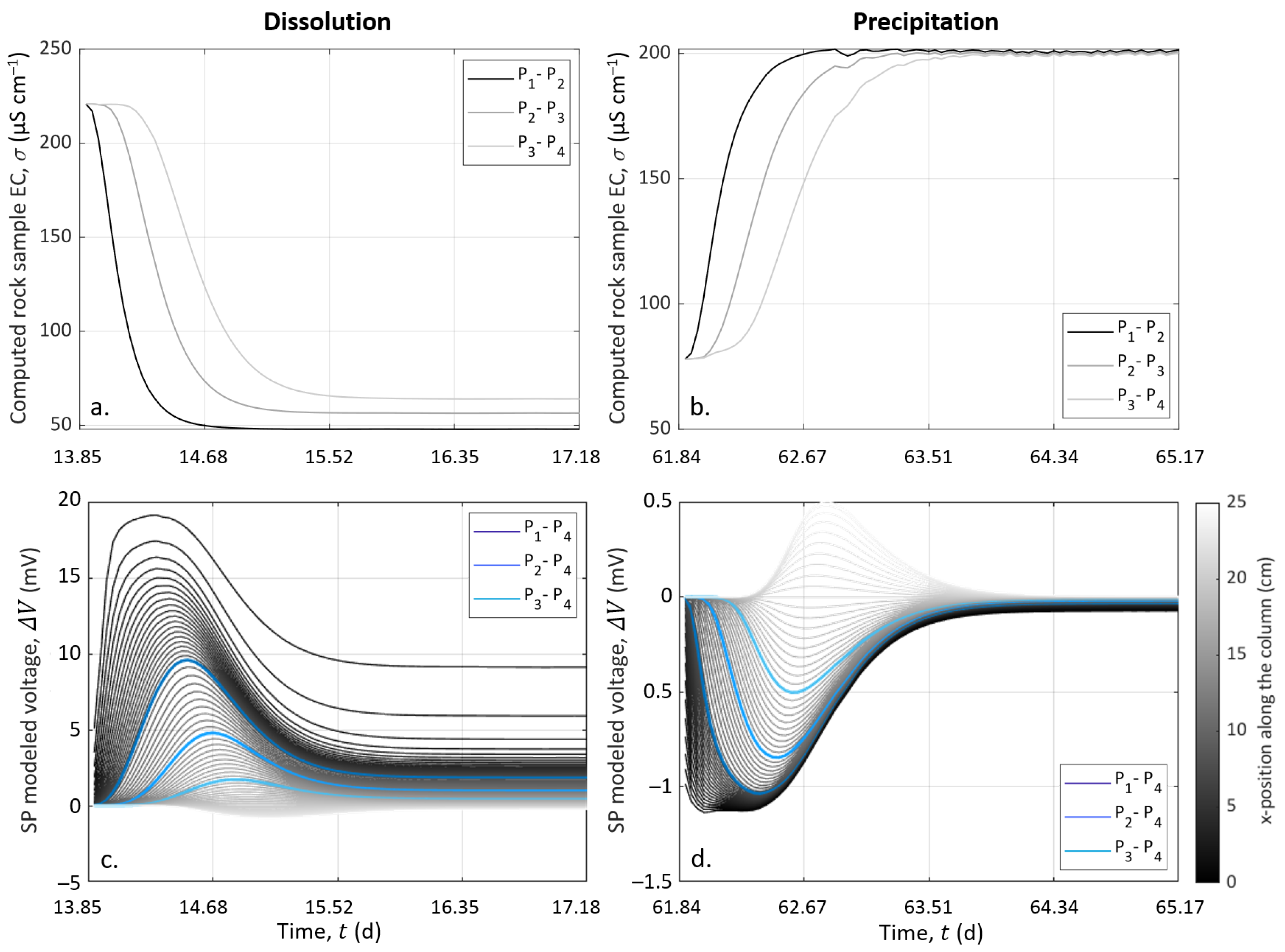
SP data and simulated electro-diffusive potential are presented in Figure 8. In Figure 8a,b, the data are plotted after removing the decrease, assuming that it is a linear function, and time zero corresponds to the start of the injection of S1 and S2 to dissolve and precipitate, respectively. The modeled electrical potential is presented in Figure 8c,d.
For both dissolution and precipitation, the modeled curves present variations that are fairly similar to the SP measurements, although not identical. Furthermore, we observed that the modeled peaks were two-times larger than the measurements in the case of dissolution. We think that the model is better adjusted in case of precipitation than in the case of dissolution because of CO degassing, which affected the system during dissolution. This degassing was not taken into account in the CrunchFlow simulation. Compared to the experimental data (see Figure 7a), this led to higher concentrations of hydrogen protons (H), while their mobility was much higher than for the other ions (see Table 2). This excess of mobile hydrogen protons exaggerated the electro-diffusive amplitude.
Our 1D approach contains some simplifications, which also explain the differences between the measured and the modeled curves. Indeed, electrical methods are integrative; thus, the model does not consider the column width, while it is worth 40% of the column length. Therefore, potential 3D effects around the fluid injection point were not considered. Furthermore, the porous medium was considered an effective medium, where the formation of a preferential path was neglected, while the sensitivity of the electrodes was not homogeneous over the entire volume of the column. Nevertheless, this workflow, without additional parameters for amplitude adjustment, provides results close to the range of experimental data and temporal variations. This workflow could be used for other purposes addressing multi-species reactive transport and mixing, e.g., [79].
4.5. Location of the Reactive Zone
CrunchFlow simulation, in addition to the ionic concentrations, resolves the time and spatial porosity evolution. Figure 9a shows the difference in porosity along the column at the end of each simulation. One can observe that the porosity changes were small, with a maximal increase of 0.1% for dissolution and a maximal decrease of −0.005% for precipitation. Besides, only a few centimeters at the column entrance were affected by these changes in porosity (gray rectangle in Figure 9a). We are rather confident in these results since the measured Ca concentrations were well reproduced by the simulations (Figure 6 and Figure 7) and the porosity changes were consistent with the low porosity evolution (see Section 4.2). Moreover, previous studies have shown that the injection of a strong acid, such as HCl, through a calcite column favors a face dissolution profile [70]. Thus, most dissolution and precipitation occurred in this portion of the column and did not reach the portion equipped with the measurement electrodes. Consequently, the transient variations of the SP signal come from the fact that all dissolution and precipitation occurred at the entrance of the column and did not induce a sufficient chemical imbalance. This localization of the dissolution and precipitation at the column inlet also explained the low reactive surface area used in the model to reproduce the outlet calcium concentration. This very low reactive surface area compared to the total fluid–rock interface (several orders of magnitude lower) indicates that only a very small part of the calcite reacted with the injected solution.
Using the computation of the pore water EC based on the ionic mobilities (Equation (11)), we were not limited to the measurement of the sample EC at the three locations along the column, but can compute the model on all x-locations along the column defined for the CrunchFlow simulation. In Figure 9b,c, the electro-diffusive potential distribution along the column is represented for successive time steps of the CrunchFlow simulation. For the latest timings, the shapes of the curves present variations similar to the trends observed for the porosity simulated with CrunchFlow (Figure 9a). These observations led to the same conclusions concerning the reactive zone limited to the column inlet.
Thus, this experimental device with multichannel monitoring allows the discretization of the electrical response related to the reactive transport processes and following in time and space the evolution of this reactive porous medium. Thanks to the interpretation brought by the workflow developed for this study, this SP monitoring can be quantitatively interpreted, and we can extrapolate the measurements over non-equipped portions of the sample. This theoretical contribution, validated by this experimentation, is of interest for many issues. Regarding calcite precipitation, it is important to follow its effects in civil engineering, for example in the face of cement carbonation or for soil consolidation, e.g., [80,81]. Concerning dissolution, it is a process monitored for the exploitation of reservoirs and the improvement of their properties, e.g., [82]. In the field of remediation, dissolution and precipitation are interesting to monitor because carbonate rocks can act as reactive barriers trapping contaminants, e.g., [83].
5. Conclusions
In this study, we developed the first geochemical–geophysical fully coupled multi-species numerical workflow to predict the SP electrochemical response to calcite dissolution or precipitation. This workflow consists of the computation of the electro-diffusive potential using spatial and temporal distributions of ionic concentrations obtained from reactive transport simulations. To assess the accuracy of this model, we compared these numerical results with SP monitoring of calcite dissolution or precipitation carried out for this study. The fairly good match between the numerical simulation and the experimental data showed the efficiency of the numerical workflow. Therefore, we believe that studies addressing multi-species reactive transport and mixing could use this workflow with SP monitoring to improve the in situ characterization of these processes.
The experiment was performed on a column packed with calcite grains and equipped to monitor three geo-electrical properties: pore water EC, sample EC, and SP voltage, together with chemical analysis on outlet pore water samples (alkalinity, pH, and major ion concentrations). All of these monitored properties show clear correlated variations, suggesting that chemical reactions with calcite grains occurred at the entrance of the column. This experimental evidence was confirmed by reactive transport simulation. Consequently, this experimental setup enables the joint use of multiple geo-electrical methods, which, once compared with chemical analyses, can be quantitatively interpreted. However, the chemical reactions with calcite grains occurred too close to the entrance to be fully monitored. Further study, with a revised experimental setup, would be needed. In addition, calcite dissolution induced by weak acid injection would be a scenario closer to field conditions and would lead to a more distributed dissolution profile along with the porous medium. This experimental protocol will be considered for future work.
This work clearly shows the interest in geo-electrical methods to non-intrusively monitor reactive transport processes. Thanks to our new fully coupled approach, this study allowed us to locate the reactive zone and better understand the impact of the reactivity on the porous medium petrophysical properties. Future works will improve this approach to provide a more quantitative tool for studying reactive transport in carbonate media.
Author Contributions
Conceptualization, F.R., D.J. and R.G.; methodology, F.R., D.J., L.L. and R.G.; software, F.R. and L.L.; validation, F.R.; formal analysis, F.R. and L.L.; investigation, F.R.; resources, D.J.; data curation, F.R.; writing—original draft preparation, F.R.; writing—review and editing, F.R., D.J., L.L. and R.G.; visualization, F.R.; supervision, D.J. and R.G.; project administration, D.J. and R.G. All authors have read and agreed to the published version of the manuscript.
Funding
This research was funded by the research project EC2CO (CNRS-INSU) StarTrek and the LabEx VOLTAIRE grant number ANR-10-LABX-100-01.
Institutional Review Board Statement
Not applicable.
Informed Consent Statement
Not applicable.
Data Availability Statement
The data used in this study are available in the zenodo repository (https://doi.org/10.5281/zenodo.4773686 accessed on 18 May 2022).
Acknowledgments
The authors also acknowledge Emmanuel Aubry for the technical support and the chemical composition analyses. The authors are also very thankful to Alexis Maineult for the donation of equipment for the continuous water conductivity measurement.
Conflicts of Interest
The authors declare no conflict of interest. The funders had no role in the design of the study; in the collection, analyses, or interpretation of the data; in the writing of the manuscript; nor in the decision to publish the results.
Sample Availability
Samples of the calcite compounds filling the column are available from the authors.
Notations
The following notations are used in this manuscript:
| Symbol | Definition (unit) |
| Alkalinity ( ) | |
| Electro-diffusive coupling coefficient () | |
| Mobility on ion ( ) | |
| C | Ionic concentration of the solution ( ) |
| Standard concentration ( ) | |
| Ionic concentration of ion ( ) | |
| Electrokinetic coupling coefficient ( ) | |
| Mean grain diameter () | |
| Diffusion coefficient of ion ( ) | |
| Time step for the calculation of the cumulative porosity () | |
| Electric voltage () | |
| E | Electric field ( ) |
| Water dynamic viscosity ( ) | |
| f | Frequency () |
| F | Formation factor (–) |
| Faraday constant ( ) | |
| Activity coefficient of the ion (–) | |
| Source current density ( ) | |
| Electrochemical coupling current density from ionic concentration gradients ( ) | |
| Electrokinetic coupling current density ( ) | |
| Total electric current density ( ) | |
| Boltzmann constant ( ) | |
| Acidity constant of bicarbonate ion (–) | |
| Acidity constant of carbonate ion (–) | |
| Hydration constant (–) | |
| Solubility product of calcite (–) | |
| Molar conductivity of ion ( ) | |
| m | Cementation exponent (–) |
| Cumulative mass of calcium (g) | |
| Angular frequency ( ) | |
| Saturation index (–) | |
| Empirical parameter for temperature compensation (–) | |
| Péclet number (–) | |
| One of the measurement electrodes | |
| Reference electrode | |
| Porosity (–) | |
| Final porosity (–) | |
| Initial porosity (–) | |
| Q | Flow rate ( ) |
| Volumetric excess charge ( ) | |
| Molar gas constant ( ) | |
| REV | Representative elementary volume |
| Calcite volumetric mass ( ) | |
| Sample EC ( ) | |
| Bulk conductivity ( ) | |
| Inlet pore water EC ( ) | |
| Outlet pore water EC ( ) | |
| Surface conductivity ( ) | |
| Pore water electrical conductivity ( ) | |
| t | Time () |
| T | Temperature () |
| Transference number (–) | |
| Temperature () | |
| U | Darcy velocity ( ) |
| v | Particle velocity ( ) |
| V | Electric potential () |
| Volume of the column () | |
| Ionic activity of the ion (–) | |
| Valence of the ion (–) |
Appendix A. Temperature Monitoring
To ensure steady conditions during the experiment, the setup was placed under air-conditioned conditions. However, to control the stability of the installation, we monitored the room temperature using a sensor from HOBO recording every . In addition, we manually recorded the inlet and outlet pore water temperatures measured by the conductivity meters. These data are presented in Figure A1.
Figure A1.
Temperature monitoring of the room (gray curve), the inlet pore water (black triangles), and the outlet pore water (blue triangle).
Figure A1.
Temperature monitoring of the room (gray curve), the inlet pore water (black triangles), and the outlet pore water (blue triangle).

We observed that the room temperature overall comprised a short range close to . However, there were plenty of high-frequency oscillations corresponding to the adjustment of the temperature with the air-conditioning system. There was also an event of a strong increase in the room temperature before Event 3, which was considered in the CrunchFlow simulation.
The pore water temperature at the inlet and outlet showed values in agreement with the room temperature. It can be noted that the temperature was slightly higher at the inlet than at the outlet, but this difference was within the range of the measurement uncertainties.
Appendix B. Electro-Diffusive Coupling Computation from Pore Water EC Computation
The electro-diffusive coupling was computed based on the interpolation of the sample EC measurements in Figure 8. However, the expression of the electro-diffusive coupling from Equation (25) can be developed using the relationship of the pore water EC with the ionic mobilities (Equation (11)), leading to
The results of the computation of the sample EC and this expression for the electro-diffusive coupling are presented in Figure A2. These results are in good agreement with the measured sample EC and SP voltage presented in Figure 5.
Using the definition of the pore water EC based on the ionic mobilities, we can compute the model on all x-locations along the column defined for the CrunchFlow simulation. This shows the continuous evolution in time and space of the modeled electro-diffusive potential.
References
- Goldscheider, N.; Meiman, J.; Pronk, M.; Smart, C. Tracer tests in karst hydrogeology and speleology. Int. J. Speleol. 2008, 37, 27–40. [Google Scholar] [CrossRef] [Green Version]
- Hubbard, S.S.; Linde, N. 2.15-Hydrogeophysics. In Treatise on Water Science; Wilderer, P., Ed.; Elsevier: Oxford, UK, 2011; pp. 401–434. [Google Scholar] [CrossRef]
- Revil, A.; Karaoulis, M.; Johnson, T.; Kemna, A. Some low-frequency electrical methods for subsurface characterization and monitoring in hydrogeology. Hydrogeol. J. 2012, 20, 617–658. [Google Scholar] [CrossRef]
- Binley, A.; Hubbard, A.S.; Huisman, J.A.; Revil, A.; Robinson, D.A.; Singha, K.; Slater, L.D. The emergence of hydrogeophysics for improved understanding of subsurface processes over multiple scales. Water Resour. Res. 2015, 51, 3837–3866. [Google Scholar] [CrossRef] [PubMed] [Green Version]
- Chen, Z.; Goldscheider, N.; Auler, A.S.; Bakalowicz, M. The World karst aquifer mapping project: Concept, mapping procedure and map of Europe. Hydrogeol. J. 2017, 25, 771–785. [Google Scholar] [CrossRef] [Green Version]
- Luquot, L.; Gouze, P. Experimental determination of porosity and permeability changes induced by injection of CO2 into carbonate rocks. Chem. Geol. 2009, 265, 148–159. [Google Scholar] [CrossRef]
- Cherubini, A.; Garcia, B.; Cerepi, A.; Revil, A. Influence of CO2 on the electrical conductivity and streaming potential of carbonate rocks. J. Geophys. Res. Solid Earth 2019, 124, 10056–10073. [Google Scholar] [CrossRef] [Green Version]
- Kačaroǧlu, F. Review of groundwater pollution and protection in karst areas. Water Air Soil Pollut. 1999, 113, 337–356. [Google Scholar] [CrossRef]
- Bakalowicz, M. Karst groundwater: A challenge for new resources. Hydrogeol. J. 2005, 13, 148–160. [Google Scholar] [CrossRef]
- Montanari, D.; Minissale, A.; Doveri, M.; Gola, G.; Trumpy, E.; Santilano, A.; Manzella, A. Geothermal resources within carbonate reservoirs in western Sicily (Italy): A review. Earth Sci. Rev. 2017, 169, 180–201. [Google Scholar] [CrossRef]
- Burchette, T.P. Carbonate rocks and petroleum reservoirs: A geological perspective from the industry. Geol. Soc. Lond. Spec. Publ. 2012, 370, 17–37. [Google Scholar] [CrossRef]
- Drew, D.; Lamoreaux, P.E.; Coxon, C.; Wess, J.W.; Slattery, L.D.; Bosch, A.P.; Hötzl, H. Karst Hydrogeology and Human Activities: Impacts, Consequences and Implications: IAH International Contributions to Hydrogeology 20, 5th ed.; Drew, D., Hötzl, H., Eds.; Routledge: London, UK, 2017. [Google Scholar] [CrossRef]
- Buckerfield, S.J.; Quilliam, R.S.; Bussiere, L.; Waldron, S.; Naylor, L.A.; Li, S.; Oliver, D.M. Chronic urban hotspots and agricultural drainage drive microbial pollution of karst water resources in rural developing regions. Sci. Total Environ. 2020, 744, 140898. [Google Scholar] [CrossRef] [PubMed]
- Jouniaux, L.; Maineult, A.; Naudet, V.; Pessel, M.; Sailhac, P. Review of self-potential methods in hydrogeophysics. Comptes Rendus Geosci. 2009, 341, 928–936. [Google Scholar] [CrossRef] [Green Version]
- Revil, A.; Jardani, A. The Self-Potential Method: Theory and Applications in Environmental Geosciences; Cambridge University Press: New York, NY, USA, 2013. [Google Scholar]
- Jougnot, D.; Roubinet, D.; Guarracino, L.; Maineult, A. Modeling streaming potential in porous and fractured media, description and benefits of the effective excess charge density approach. In Advances in Modeling and Interpretation in Near Surface Geophysics; Biswas, A., Sharma, S., Eds.; Springer Geophysics; Springer: Cham, Switzerland, 2020; Chapter 4; pp. 61–96. [Google Scholar] [CrossRef] [Green Version]
- Guichet, X.; Jouniaux, L.; Catel, N. Modification of streaming potential by precipitation of calcite in a sand-water system: Laboratory measurements in the pH range from 4 to 12. Geophys. J. Int. 2006, 166, 445–460. [Google Scholar] [CrossRef] [Green Version]
- Hidayat, M.; Sarmadivaleh, M.; Derksen, J.; Vega-Maza, D.; Iglauer, S.; Vinogradov, J. Zeta potential of CO2-rich aqueous solutions in contact with intact sandstone sample at temperatures of 23 °C and 40 °C and pressures up to 10.0 MPa. J. Colloid Interface Sci. 2022, 607, 1226–1238. [Google Scholar] [CrossRef] [PubMed]
- Revil, A. Ionic diffusivity, electrical conductivity, membrane and thermoelectric potentials in colloids and granular porous media: A unified model. J. Colloid Interface Sci. 1999, 212, 503–522. [Google Scholar] [CrossRef]
- Maineult, A.; Bernabé, Y.; Ackerer, P. Detection of advected concentration and pH fronts from self-potential measurements. J. Geophys. Res. 2005, 110, B11205. [Google Scholar] [CrossRef]
- Korom, S.F.; Seaman, J.C. When “conservative” anionic tracers aren’t. Groundwater 2012, 50, 820–824. [Google Scholar] [CrossRef]
- Graham, M.T.; MacAllister, D.J.; Vinogradov, J.; Jackson, M.D.; Butler, A.P. Self-potential as a predictor of seawater intrusion in coastal groundwater boreholes. Water Resour. Res. 2018, 54, 6055–6071. [Google Scholar] [CrossRef] [Green Version]
- MacAllister, D.J.; Jackson, M.D.; Butler, A.P.; Vinogradov, J. Remote detection of saline intrusion in a coastal aquifer using borehole measurements of self-potential. Water Resour. Res. 2018, 54, 1669–1687. [Google Scholar] [CrossRef] [Green Version]
- Gulamali, M.Y.; Leinov, E.; Jackson, M.D. Self-potential anomalies induced by water injection into hydrocarbon reservoirs. Geophysics 2011, 76, F283–F292. [Google Scholar] [CrossRef] [Green Version]
- Revil, A.; Leroy, P. Constitutive equations for ionic transport in porous shales. J. Geophys. Res. 2004, 109, B03208. [Google Scholar] [CrossRef]
- Linde, N.; Doetsch, J.; Jougnot, D.; Genoni, O.; Dürst, Y.; Minsley, B.J.; Vogt, T.; Pasquale, N.; Luster, J. Self-potential investigations of a gravel bar in a restored river corridor. Hydrol. Earth Syst. Sci. 2011, 15, 729–742. [Google Scholar] [CrossRef] [Green Version]
- Bautista-Anguiano, J.; Torres-Verdin, C. Estimation of in situ hydrocarbon saturation of porous rocks fromborehole measurements of spontaneous potential. Geophysics 2020, 85, D199–D217. [Google Scholar] [CrossRef]
- Revil, A.; Linde, N. Chemico-electromechanical coupling in microporous media. J. Colloid Interface Sci. 2006, 302, 682–694. [Google Scholar] [CrossRef]
- Revil, A.; Jougnot, D. Diffusion of ions in unsaturated porous materials. J. Colloid Interface Sci. 2008, 319, 226–235. [Google Scholar] [CrossRef]
- Plummer, L.N.; Busenberg, E. The solubilities of calcite, aragonite and vaterite in CO2-H2O solutions between 0 and 90 °C, and an evaluation of the aqueous model for the system CaCO3-CO2-H2O. Geochim. Cosmochim. Acta 1982, 46, 1011–1040. [Google Scholar] [CrossRef]
- Cohen, E.R.; Cvitaš, T.; Frey, J.G.; Holmström, B.; Kuchitsu, K.; Marquardt, R.; Mills, I.; Pavese, F.; Quack, M.; Stohner, J.; et al. Quantities, Units and Symbols in Physical Chemistry, 3rd ed.; Royal Society of Chemistry: Cambridge, UK, 2007. [Google Scholar]
- De Marsily, G. Quantitative Hydrogeology: Groundwater Hydrology for Engineers, 2nd ed.; Paris School of Mines: Fontainebleau, France, 1986; p. 440. [Google Scholar]
- Bear, J. Dynamics of Fluids in Porous Media; American Elsevier: New York, NY, USA, 1988. [Google Scholar]
- Vialle, S.; Contraires, S.; Zinzsner, B.; Clavaud, J.B.; Mahiouz, K.; Zuddas, P.; Zamora, M. Percolation of CO2-rich fluids in a limestone sample: Evolution of hydraulic, electrical, chemical, and structural properties. J. Geophys. Res. Solid Earth 2014, 119, 2828–2847. [Google Scholar] [CrossRef]
- Leger, M.; Roubinet, D.; Jamet, M.; Luquot, L. Impact of hydro-chemical conditions on structural and hydro-mechanical properties of chalk samples during dissolution experiments. Chem. Geol. 2022, 594, 120763. [Google Scholar] [CrossRef]
- McCleskey, R.B.; Nordstrom, D.K.; Ryan, J.N. Comparison of electrical conductivity calculation methods for natural waters. Limnol. Oceanogr. Methods 2012, 10, 952–967. [Google Scholar] [CrossRef]
- Atkins, P.; de Paula, J. Atkins’ Physical Chemistry; Oxford University Press: New York, NY, USA, 1994. [Google Scholar]
- Robinson, R.A.; Chia, C.L. The diffusion coefficient of calcium chloride in aqueous solution at 25. J. Am. Chem. Soc. 1952, 74, 2776–2777. [Google Scholar] [CrossRef]
- Gregory, T.M.; Chow, L.C.; Carey, C.M. A mathematical model for dental caries: A coupled dissolution-diffusion process. J. Res. Natl. Inst. Stand. Technol. 1991, 96, 593–604. [Google Scholar] [CrossRef] [PubMed]
- Parkhurst, D.L.; Appelo, C.A.J. Description of Input and Examples for PHREEQC Version 3: A Computer Program for Speciation, Batch-Reaction, One-Dimensional Transport, and Inverse Geochemical Calculations; Technical Report; US Geological Survey: Denver, CO, USA, 2013. [CrossRef] [Green Version]
- Hunter, R.J. Zeta Potential in Colloid Science: Principles and Applications; Academic Press London: London, UK, 1981; Volume 2, p. 391. [Google Scholar] [CrossRef]
- Chelidze, T.L.; Gueguen, Y. Electrical spectroscopy of porous rocks: A review-I. Theoretical models. Geophys. J. Int. 1999, 137, 1–15. [Google Scholar] [CrossRef]
- Leroy, P.; Revil, A. A triple layer model of the surface electrochemical properties of clay minerals. J. Colloid Interface Sci. 2004, 270, 371–380. [Google Scholar] [CrossRef] [PubMed]
- Bolève, A.; Crespy, A.; Revil, A.; Janod, F.; Mattiuzzo, J.L. Streaming potentials of granular media: Influence of the Dukhin and Reynolds numbers. J. Geophys. Res. 2007, 112, 204–217. [Google Scholar] [CrossRef] [Green Version]
- Soueid Ahmed, A.; Revil, A.; Abdulsamad, F.; Steck, B.; Vergniault, C.; Guihard, V. Induced polarization as a tool to non-intrusively characterize embankment hydraulic properties. Eng. Geol. 2020, 271, 105604. [Google Scholar] [CrossRef]
- Waxman, M.H.; Smits, L.J.M. Electrical conductivities in oil bearing shaly sands. Soc. Pet. Eng. J. 1968, 8, 107–122. [Google Scholar] [CrossRef]
- Weller, A.; Slater, L.; Nordsiek, S. On the relationship between induced polarization and surface conductivity: Implications for petrophysical interpretation of electrical measurements. Geophysics 2013, 78, D315–D325. [Google Scholar] [CrossRef]
- Revil, A.; Kessouri, P.; Torres-Verdin, C. Electrical conductivity, induced polarization, and permeability of the fontainebleau sandstone. Geophysics 2014, 79, D301–D318. [Google Scholar] [CrossRef] [Green Version]
- Rembert, F.; Jougnot, D.; Guarracino, L. A fractal model for the electrical conductivity of water-saturated porous media during mineral precipitation-dissolution processes. Adv. Water Resour. 2020, 145, 103742. [Google Scholar] [CrossRef]
- Archie, G.E. The electrical resistivity log as an aid in determining some reservoir characteristics. Trans. AIME 1942, 146, 54–62. [Google Scholar] [CrossRef]
- Pfannkuch, H.O. On the correlation of electrical conductivity properties of porous systems with viscous flow transport coefficients. Dev. Soil Sci. 1972, 2, 42–54. [Google Scholar] [CrossRef]
- Thanh, L.D.; Jougnot, D.; Phan, V.D.; Nguyen, V.N.A. A physically based model for the electrical conductivity of water-saturated porous media. Geophys. J. Int. 2019, 219, 866–876. [Google Scholar] [CrossRef]
- Berg, C.F.; Kennedy, W.D.; Herrick, D.C. Conductivity in partially saturated porous media described by porosity, electrolyte saturation and saturation-dependent tortuosity and constriction factor. Geophys. Prospect. 2022, 70, 400–420. [Google Scholar] [CrossRef]
- Sill, W.R. Self-potential modeling from primary flows. Geophysics 1983, 48, 76–86. [Google Scholar] [CrossRef]
- Jougnot, D.; Linde, N. Self-potentials in partially saturated media: The importance of explicit modeling of electrode effects. Vadose Zone J. 2013, 12, 1–21. [Google Scholar] [CrossRef] [Green Version]
- Kormiltsev, V.V.; Ratushnyak, A.N.; Shapiro, V.A. Three-dimensional modeling of electric and magnetic fields induced by the fluid flow movement in porous media. Phys. Earth Planet. Inter. 1998, 105, 109–118. [Google Scholar] [CrossRef]
- Jardani, A.; Revil, A.; Bolève, A.; Cespy, A.; Dupont, J.P.; Barrash, W.; Malama, B. Tomography of the Darcy velocity from self-potential measurements. Geophys. Res. Lett. 2007, 34, 403–408. [Google Scholar] [CrossRef] [Green Version]
- Cherubini, A.; Garcia, B.; Cerepi, A.; Revil, A. Streaming potential coupling coefficient and transport properties of unsaturated carbonate rocks. Vadose Zone J. 2018, 17, 180030. [Google Scholar] [CrossRef]
- Guarracino, L.; Jougnot, D. A physically based analytical model to describe effective excess charge for streaming potential generation in water saturated porous media. J. Geophys. Res. Solid Earth 2018, 123, 52–65. [Google Scholar] [CrossRef] [Green Version]
- Jougnot, D.; Mendieta, A.; Leroy, P.; Maineult, A. Exploring the effect of the pore size distribution on the streaming potential generation in saturated porous media, insight from pore network simulations. J. Geophys. Res. Solid Earth 2019, 124, 5315–5335. [Google Scholar] [CrossRef]
- Von Smoluchowski, M. Contribution à la théorie de l’endosmose électrique et de quelques phénomènes corrélatifs. Bull. Int. L’Académie Sci. Crac. 1903, 8, 182–200. [Google Scholar]
- Leinov, E.; Jackson, M.D. Experimental measurements of the SP response to concentration and temperature gradients in sandstones with application to subsurface geophysical monitoring. J. Geophys. Res. Solid Earth 2014, 119, 6855–6876. [Google Scholar] [CrossRef] [Green Version]
- MacAllister, D.J.; Graham, M.T.; Vinogradov, J.; Butler, A.P.; Jackson, M.D. Characterizing the self-potential response to concentration gradients in heterogeneous subsurface environments. J. Geophys. Res. Solid Earth 2019, 124, 7918–7933. [Google Scholar] [CrossRef] [Green Version]
- Henderson, P. The thermodynamics of liquid cells. Z. Für Phys. Chem. 1907, 59, 118–127. [Google Scholar] [CrossRef]
- Guggenheim, E.A. A study of cells with liquid–liquid junctions. J. Am. Chem. Soc. 1930, 52, 1315–1337. [Google Scholar] [CrossRef]
- Strathmann, H. Electrochemical and thermodynamic fundamentals. In Ion-Exchange Membrane Separation Processes; Elsevier: Amsterdam, The Netherlands, 2004; Volume 9, Chapter 2; pp. 23–88. [Google Scholar] [CrossRef]
- Daintith, J. (Ed.) A Dictionary of Chemistry, 6th ed.; Oxford University Press: Oxford, UK, 2008. [Google Scholar] [CrossRef]
- Steefel, C.I. CrunchFlow. Software for Modeling Multicomponent Reactive Flow and Transport. User’s Manual; Lawrence Berkeley National Laboratory: Berkeley, CA, USA, 2009.
- Molins, S.; Trebotich, D.; Yang, L.; Ajo-Franklin, J.B.; Ligocki, T.J.; Shen, C.; Steefel, C.I. Pore-scale controls on calcite dissolution rates from flow-through laboratory and numerical experiments. Environ. Sci. Technol. 2014, 48, 7453–7460. [Google Scholar] [CrossRef]
- Garcia-Rios, M.; Cama, J.; Luquot, L.; Soler, J.M. Interaction between CO2-rich sulfate solutions and carbonate reservoir rocks from atmospheric to supercritical CO2 conditions: Experiments and modeling. Chem. Geol. 2014, 383, 107–122. [Google Scholar] [CrossRef]
- Palandri, J.L.; Kharaka, Y.K. A Compilation of Rate Parameters of Water-Mineral Interaction Kinetics for Application to Geochemical Modeling; Technical Report; Geological Survey: Menlo Park, CA, USA, 2004.
- Schulze-Makuch, D. Longitudinal dispersivity data and implications for scaling behavior. Ground Water 2005, 43, 443–546. [Google Scholar] [CrossRef]
- Chakraborty, P.; Bhabani, S.D. Measurement and modeling of longitudinal dispersivity in undisturbed saturated soil: An experimental approach. Soil Sci. Soc. Am. J. 2018, 83, 1117–1123. [Google Scholar] [CrossRef]
- Petiau, G.; Dupis, A. Noise, temperature coefficient, and long time stability of electrodes for telluric observations. Geophys. Prospect. 1980, 28, 792–804. [Google Scholar] [CrossRef]
- Sorensen, J.A.; Glass, G.E. Ion and temperature dependence of electrical conductance for natural waters. Anal. Chem. 1987, 59, 1594–1597. [Google Scholar] [CrossRef]
- Hayashi, M. Temperature-electrical conductivity relation of water for environmental monitoring and geophysical data inversion. Environ. Monit. Assess. 2004, 96, 119–128. [Google Scholar] [CrossRef] [PubMed]
- Smart, C.C. Temperature compensation of electrical conductivity in glacial meltwaters. J. Glaciol. 1992, 38, 9–12. [Google Scholar] [CrossRef] [Green Version]
- Friedman, S.P. Soil properties influencing apparent electrical conductivity: A review. Comput. Electron. Agric. 2005, 46, 45–70. [Google Scholar] [CrossRef]
- Oliveira, T.D.S.; Blunt, M.J.; Bijeljic, B. Multispecies reactive transport in a microporous rock: Impact of flow heterogeneity and reversibility of reaction. Water Resour. Res. 2020, 56, e2020WR027317. [Google Scholar] [CrossRef]
- Gawel, K.; Wenner, S.; Edvardsen, L. Effect of carbonation on bulk resistivity of cement/carbon nanofiber composites. Constr. Build. Mater. 2021, 305, 124794. [Google Scholar] [CrossRef]
- Saneiyan, S.; Ntarlagiannis, D.; Ohan, J.; Lee, J.; Colwell, F.; Burns, S. Induced polarization as a monitoring tool for in-situ microbial induced carbonate precipitation (MICP) processes. Ecol. Eng. 2019, 127, 36–47. [Google Scholar] [CrossRef]
- Hong, D.; Cao, J.; Wu, T.; Dang, S.; Hu, W.; Yao, S. Authigenic clay minerals and calcite dissolution influence reservoir quality in tight sandstones: Insights from the central Junggar Basin, NW China. Energy Geosci. 2020, 1, 8–19. [Google Scholar] [CrossRef]
- Zhang, C.; Slater, L.; Redden, G.; Fujita, Y.; Johnson, T.; Fox, D. Spectral induced polarization signatures of hydroxide adsorption and mineral precipitation in porous media. Environ. Sci. Technol. 2012, 46, 4357–4364. [Google Scholar] [CrossRef]
Figure 1.
Numerical workflow that couples geochemical simulation (blue dashed framework) with geophysical monitoring (red dashed framework) for the computation of the electro-diffusive potential.
Figure 1.
Numerical workflow that couples geochemical simulation (blue dashed framework) with geophysical monitoring (red dashed framework) for the computation of the electro-diffusive potential.

Figure 2.
(a) Schematic drawing of the experimental setup. C and C are the current electrodes made of stainless steel, while P to P are the silver–silver chloride (Ag-AgCl) unpolarizable potential electrodes. (b) Picture of the setup during geo-electrical measurements. (c) Picture of the column, which is a Plexiglas cylinder filled with calcite grains. The tightening structure clamps the column and the current electrodes with four threaded rods between two rigid plates.

Figure 3.
Timeline of the experiment successive stages and events. Blue, pink, and green rectangles indicate the different stages: Stage I consists of the initialization to reach a stationary state close to equilibrium with calcite; Stage II corresponds to calcite dissolution with the constant injection of hydrochloric acid (solution S1); Stage III refers to calcite precipitation with the constant injection of a calcite over-saturated solution (S2). The four stars of the timeline are related to specific events. Event 0 refers to the turning on of the peristaltic pump. Event 1 refers to the connection between the inlet and outlet for recirculation of the solution in the sample. Event 2 refers to the disconnection between the inlet and outlet compartments and to the start of injecting solution S1. Event 3 refers to the start of injection of solution S2.

Figure 4.
Measurements were performed during the laboratory experiment. The dashed boxes are the delimitation of the zoomed-in views presented in Figure 5. (a) Sample EC. (b) Inlet and outlet pore water EC. The data gap of the outlet water EC curve comes from an acquisition interruption due to the conductivity meter flat battery. (c) SP curves were measured on three channels of acquisition, using electrode P as the reference. The white squares represent the interruption of SP acquisition to measure sample EC instead. (d–f) pH, calcium concentration , and alkalinity of the water sampled at the outlet of the column, respectively. (g) Saturation index for calcite computed from outlet pore water chemical analysis.
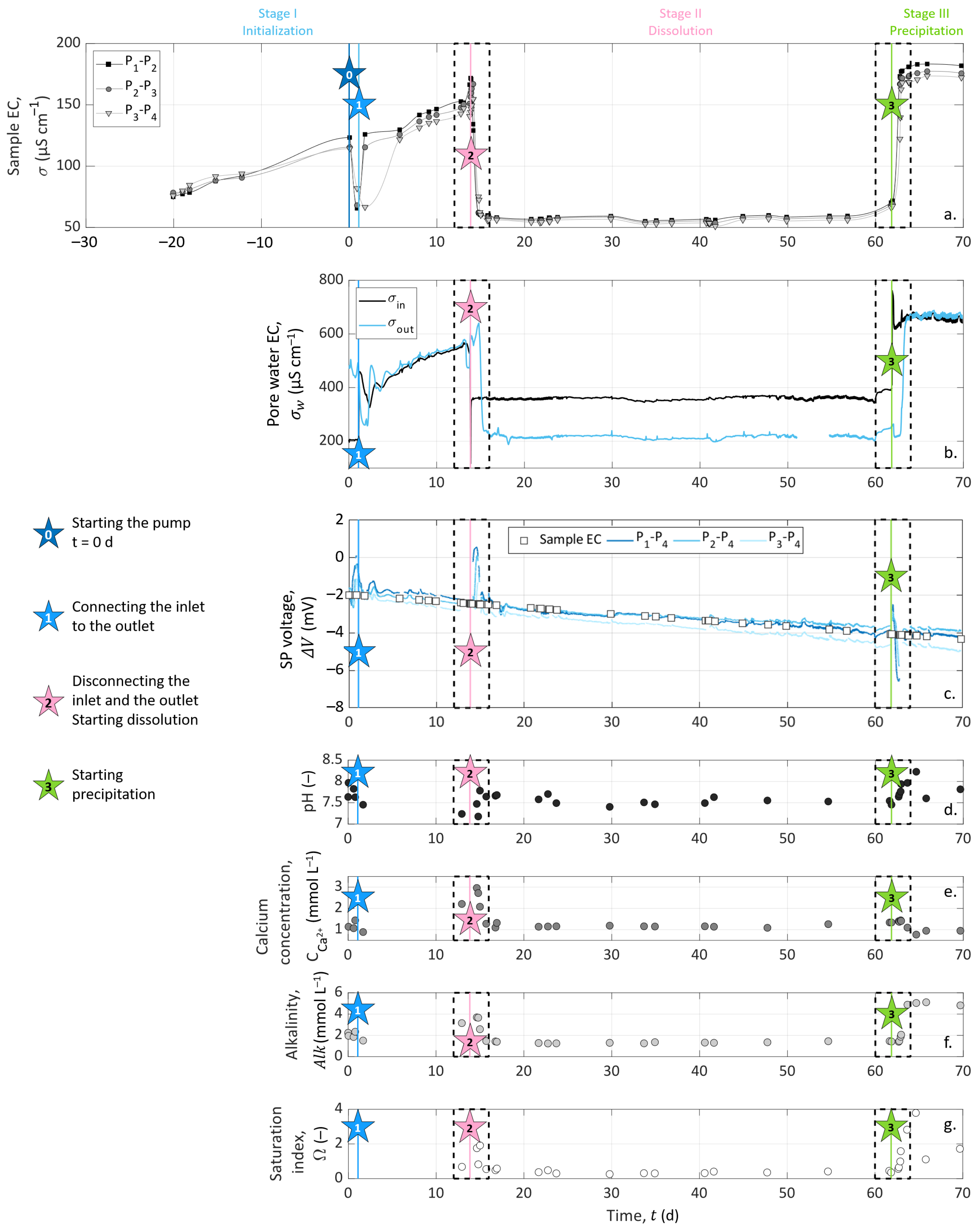
Figure 5.
Zoomed views of Figure 4 centered on Events 2 and 3. (a,b) Sample EC measured on three channels of acquisition corresponding to different dipoles of potential electrodes. (c,d) Inlet and outlet pore water EC. (e,f) SP curves measured on three channels of acquisition corresponding to different dipoles of potential electrodes, using electrode P as the reference. The white squares represent the interruption of SP acquisition to measure sample EC instead. (g,h) Calcium concentration, alkalinity, and pH variations.
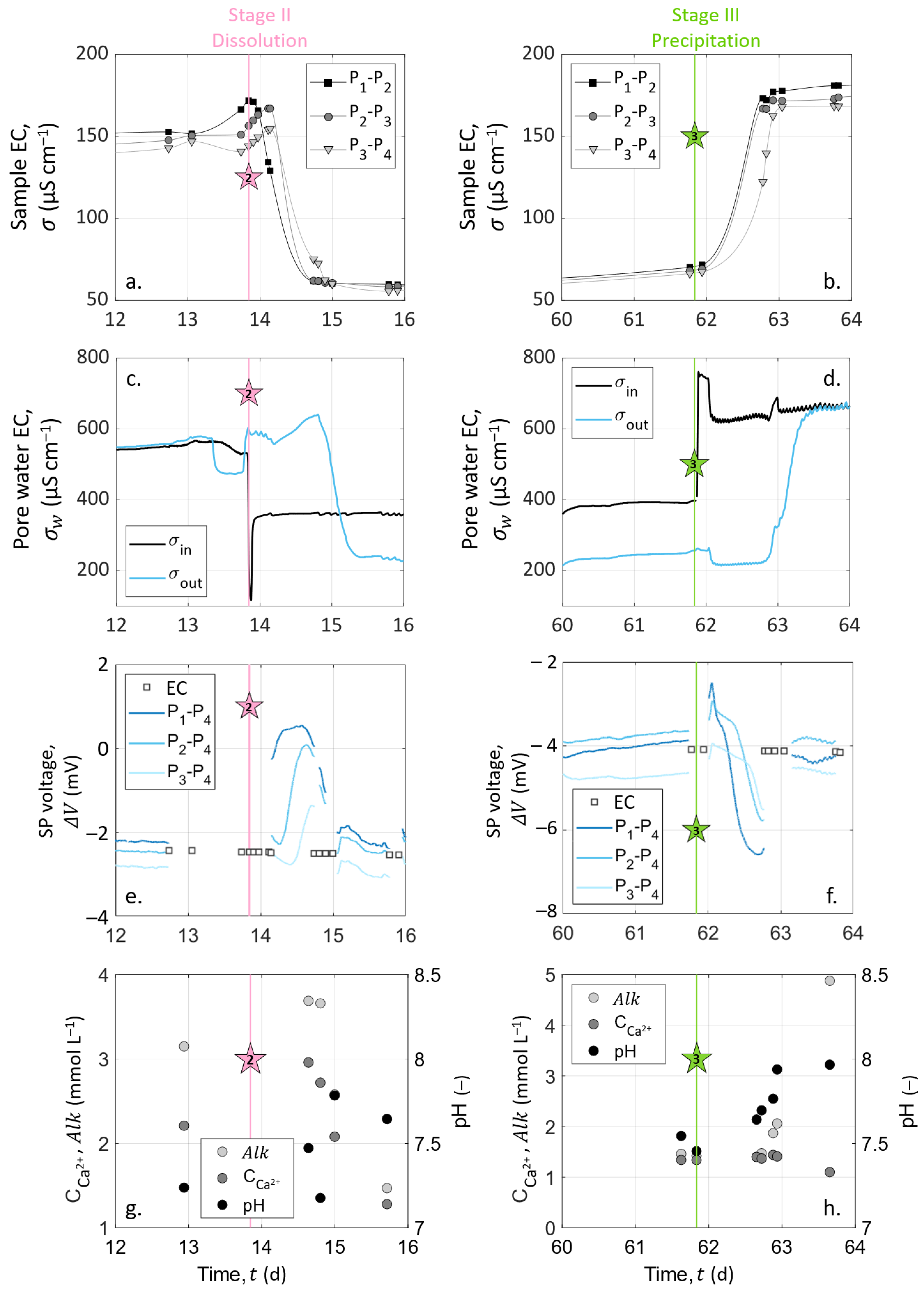
Figure 6.
Porosity and cumulative mass of dissolved calcium evolution during the experiment.

Figure 7.
Measured and modeled pH, calcium concentration, and bicarbonate concentration. The data points come from the chemical analyses conducted on the outlet pore water samples, and the curves are obtained from CrunchFlow simulations. (a,c,e) Comparison between the measured data and the corresponding simulations for dissolution. (b,d,f) Comparison between the measured data and the corresponding simulations for precipitation.

Figure 8.
(a,b) SP data were corrected from the linear decrease generated by the intrinsic potential drift of the reference electrode P. Time zero corresponds to the timing of Events 2 (injection of solution S1) and 3 (injection of solution S2), respectively. (c,d) Electro-diffusive voltage computed from the numerical workflow.
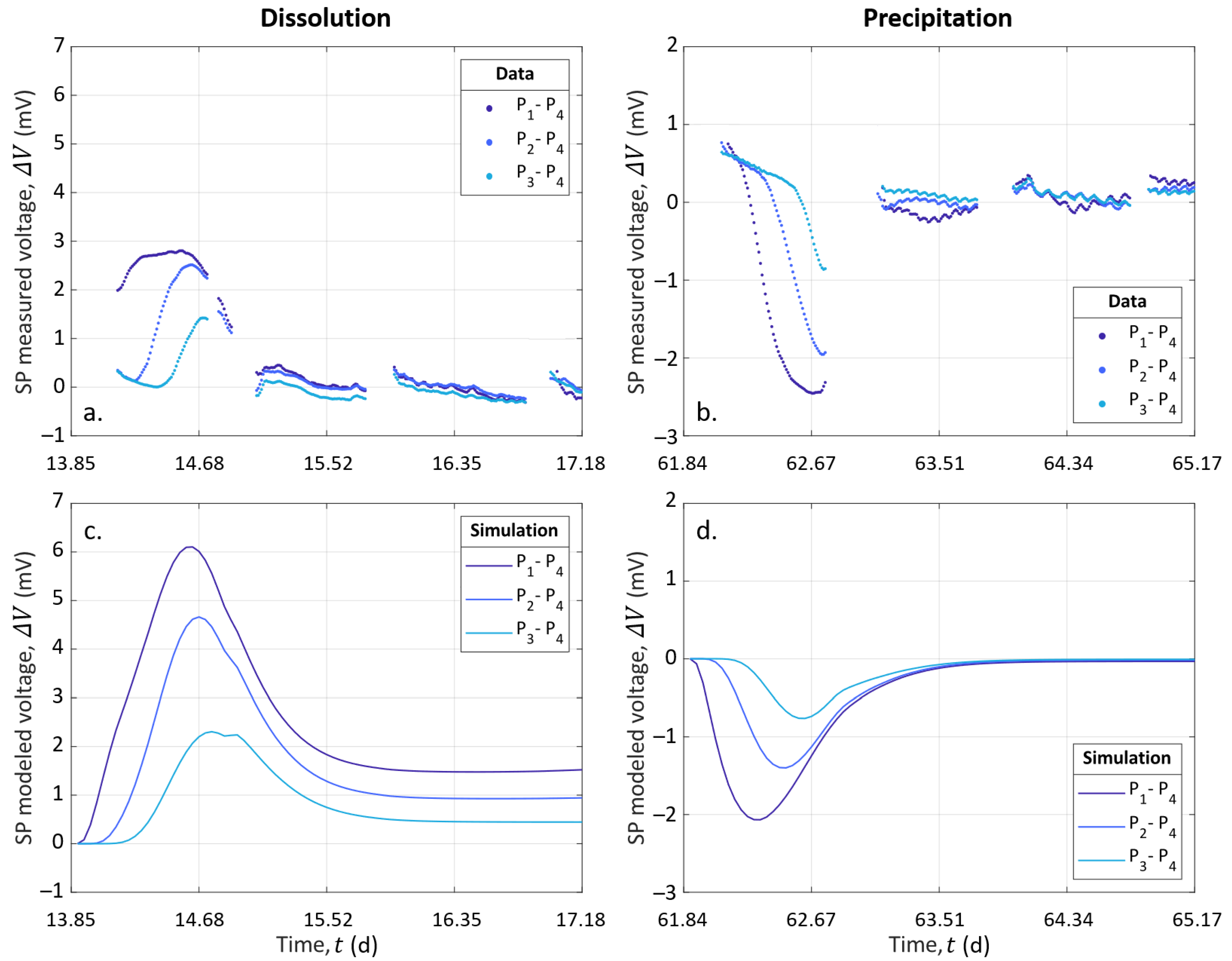
Figure 9.
Representations along the column. Locations of measurement electrodes P, P, P, and P are indicated on top of each graphic. (a) Porosity difference along the column for CrunchFlow simulations of calcite dissolution and precipitation. (b) The SP voltage is modeled at different time steps during calcite dissolution. (c) The SP voltage is modeled at different time steps during calcite precipitation.


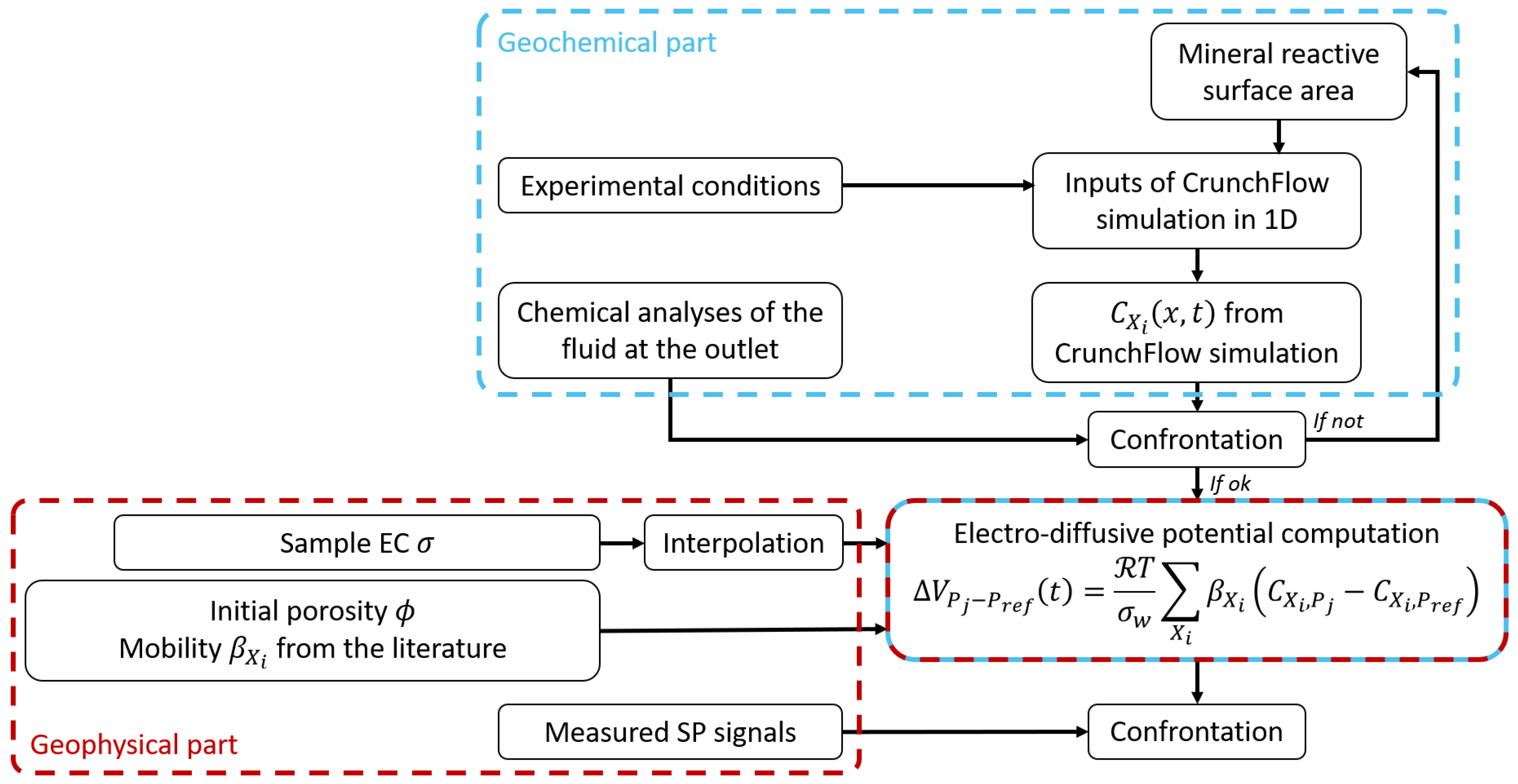
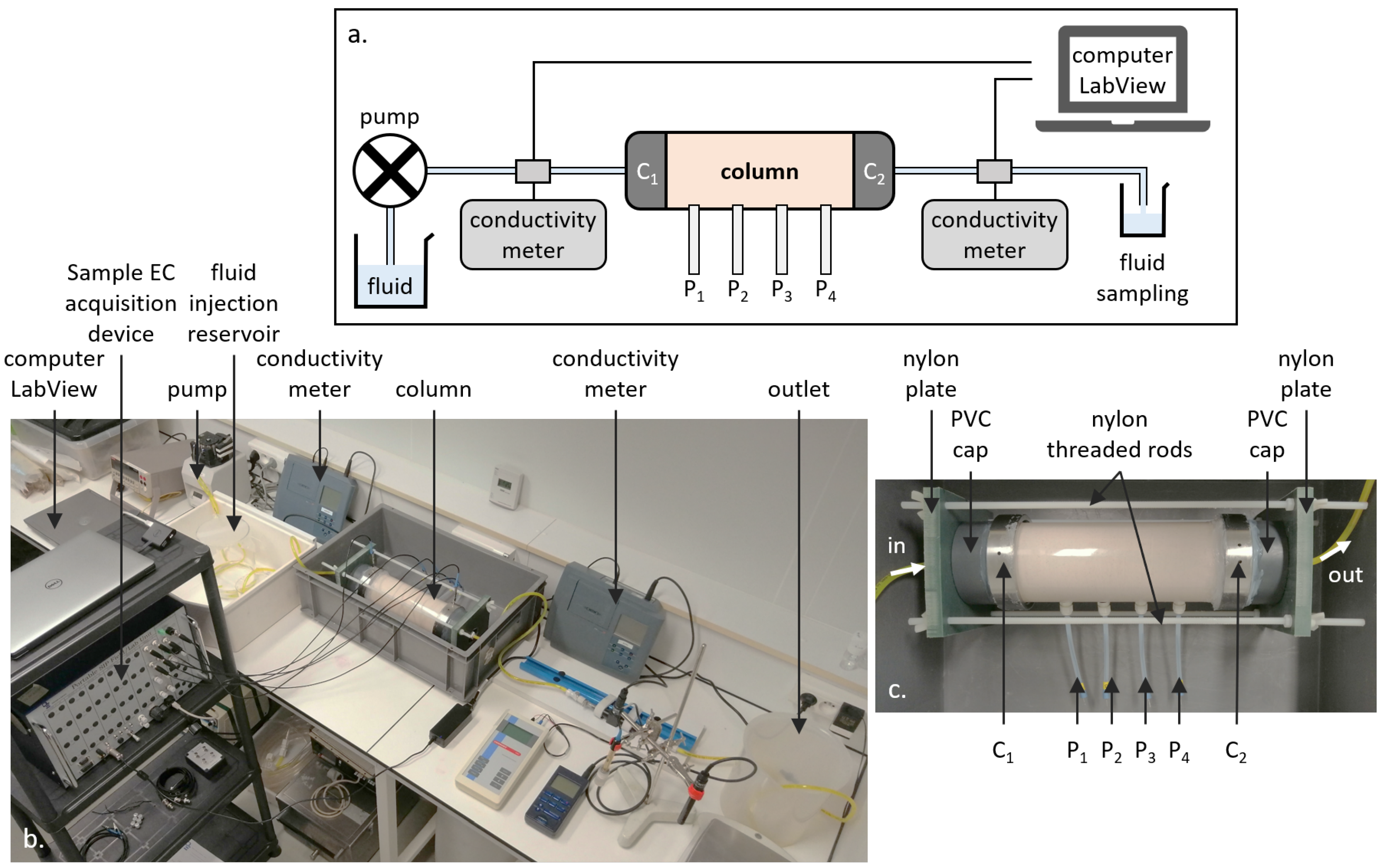
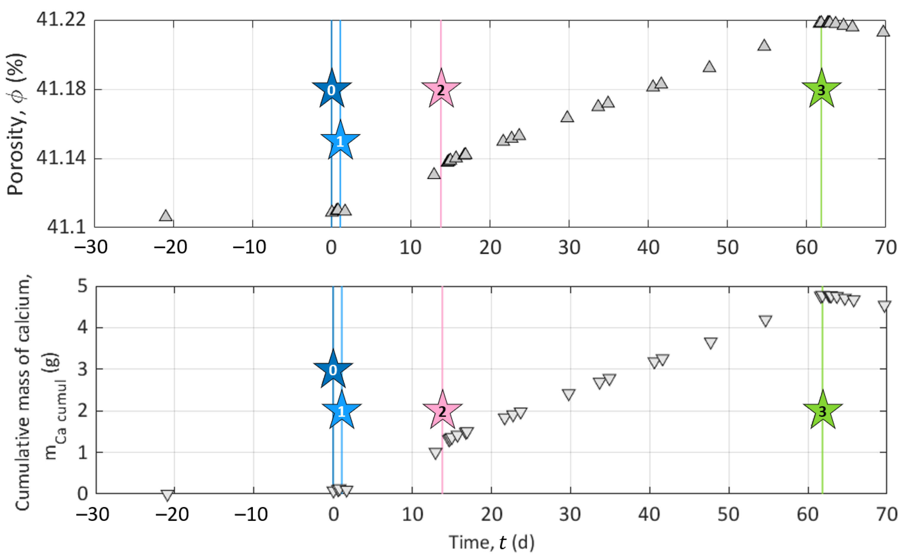
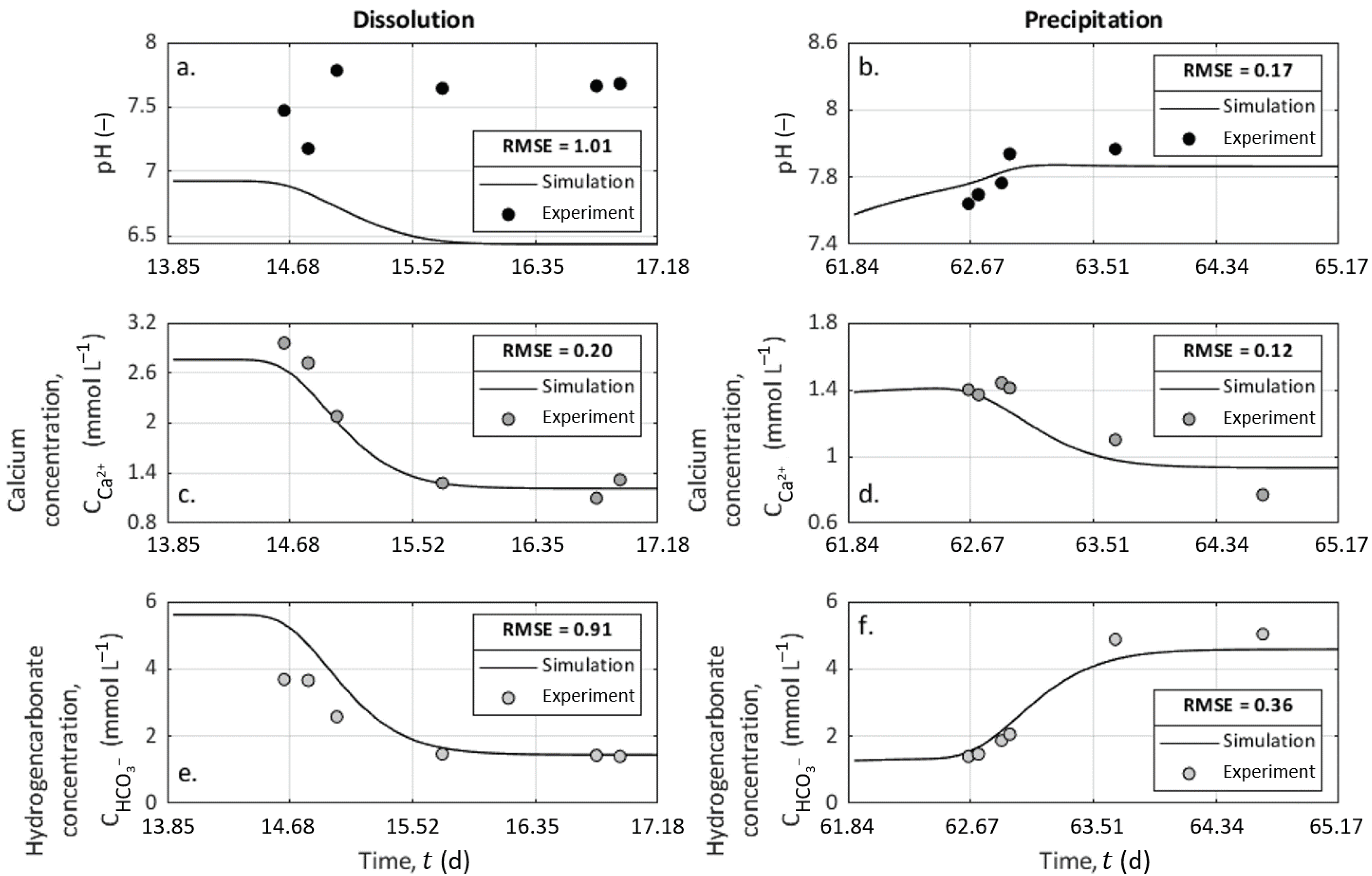
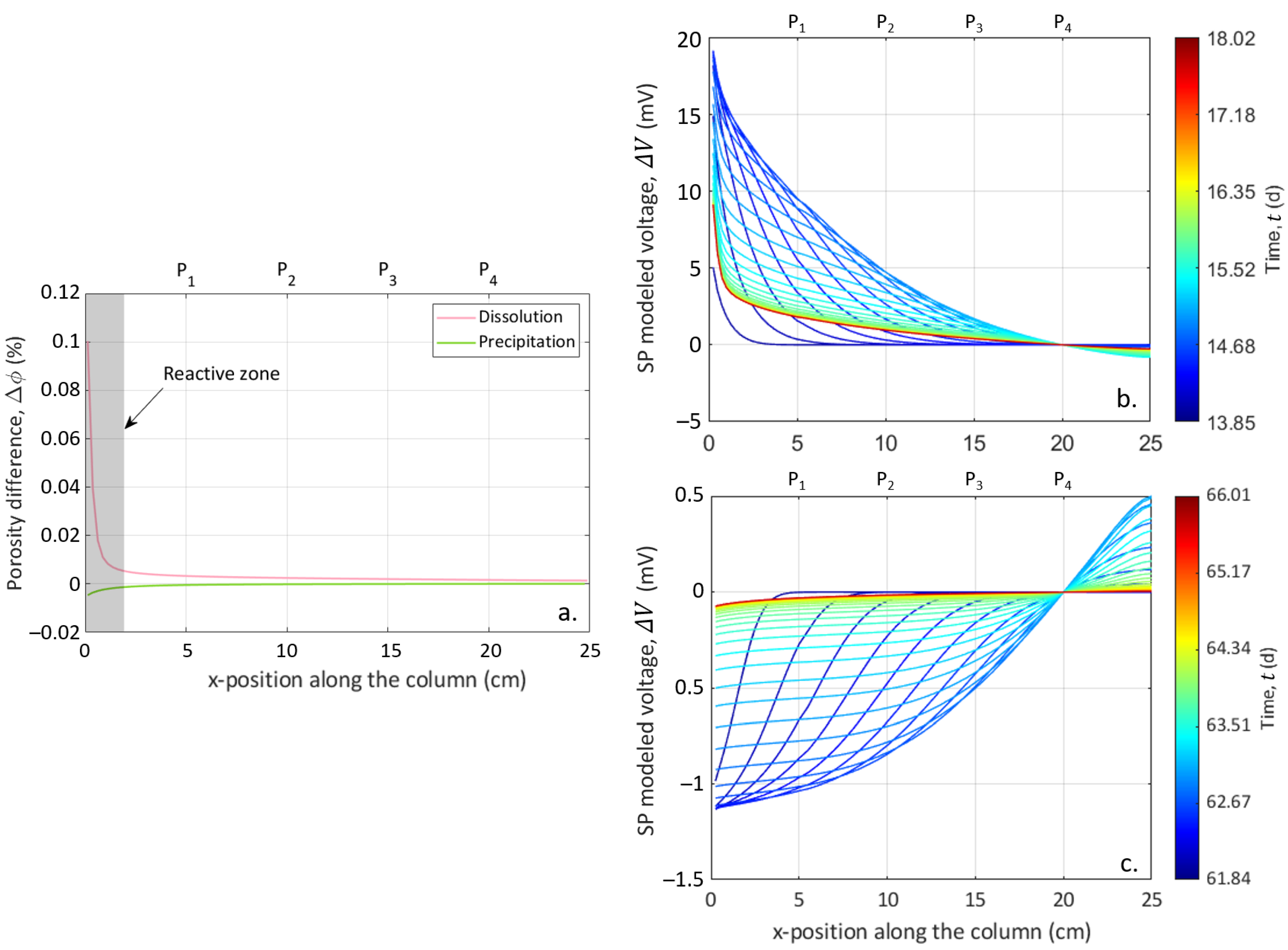
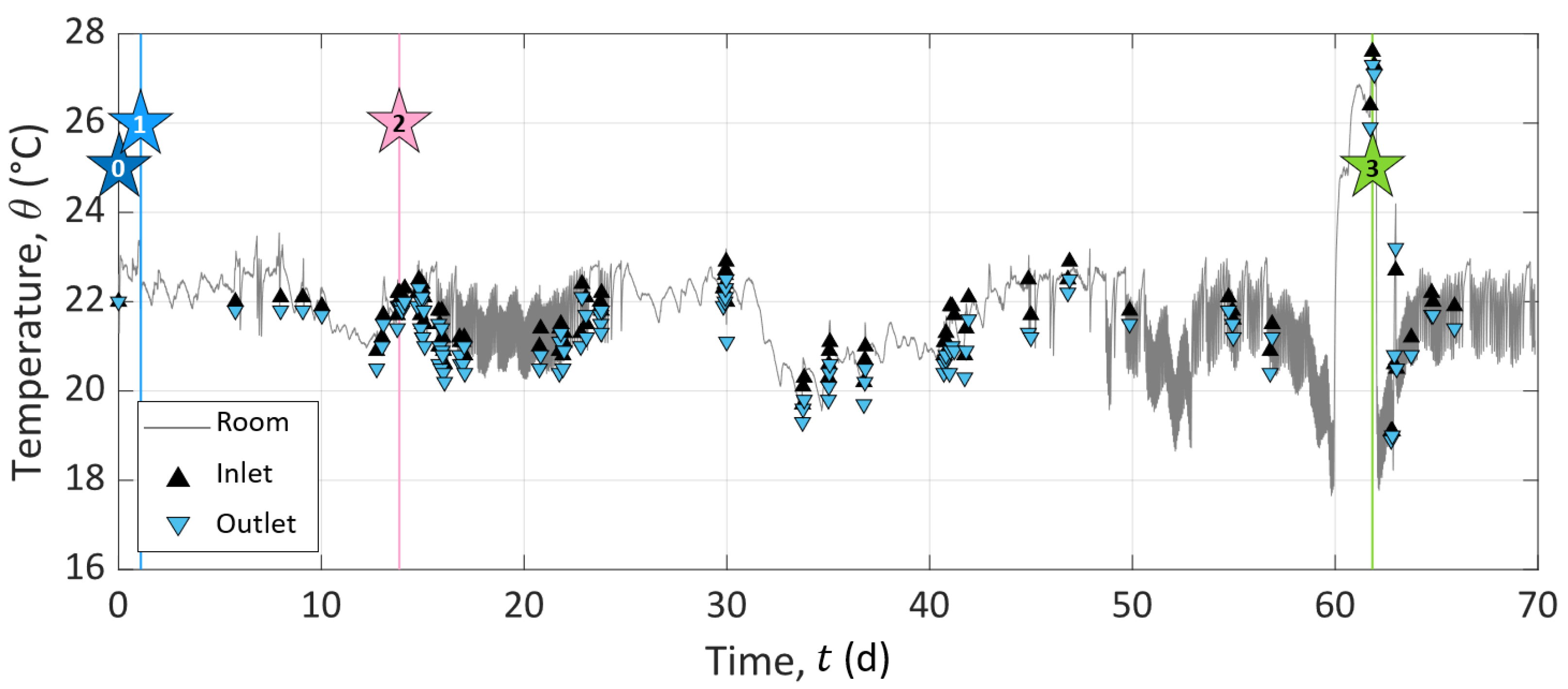
Table 1.
Equations for the carbonate system in equilibrium with calcite in aqueous media, e.g., [30].
Table 1.
Equations for the carbonate system in equilibrium with calcite in aqueous media, e.g., [30].
| Equations | Thermodynamic Constants (25 C) |
|---|---|
| CO + HO ↔ HCO | |
| HCO ↔ H + HCO | |
| HCO ↔ H + CO | |
| Ca + CO ↔ CaCO |
Table 2.
Values of molar conductivity and mobility of the ionic species considered in this study. These values are taken from the literature [38,39,40].
| Ionic Species | Molar Conductivity | Mobility |
|---|---|---|
| ( ) | ( ) | |
| Ca | 119.1 | 0.62 |
| H | 349.6 | 3.62 |
| Na | 50.0 | 0.52 |
| CaCl | 50.9 | 0.53 |
| CaHCO | 19.0 | 0.20 |
| CaOH | 39.1 | 0.41 |
| Cl | 76.2 | 0.79 |
| HCO | 44.3 | 0.46 |
| CO | 143.5 | 0.74 |
| NaCO | 22.0 | 0.23 |
| HO | 197.9 | 2.05 |
Table 3.
Input parameters used for the CrunchFlow simulations. Input pore water concentration values come from the outlet pore water chemical analyses, and inlet solution concentration values come from S1 and S2 compositions.
Table 3.
Input parameters used for the CrunchFlow simulations. Input pore water concentration values come from the outlet pore water chemical analyses, and inlet solution concentration values come from S1 and S2 compositions.
| Experiment | Dissolution | Precipitation |
|---|---|---|
| Rock composition | Calcite | |
| Reactive specific surface area (m/m) | 1.5 | |
| Temperature () | from experimental measurements | |
| Initial pore water properties | ||
| pH | 6.9 | 7.4 |
| ( ) | 2.9 | 1.4 |
| ( ) | 7.1 | 1.4 |
| ( ) | 2.0 | 1.0 |
| ( ) | 2.0 | 0.0 |
| Inlet solutions properties | ||
| pH | 3.0 | 8.5 |
| ( ) | 1.2 | |
| ( ) | 1.4 | 4.8 |
| ( ) | 1.0 | 2.4 |
| ( ) | 4.9 | |
| Flow and transport properties | ||
| Effective diffusion coefficient ( ) | 3.0 | |
| Dispersivity () | 0.9 | |
| Darcy velocity ( ) | 2.7 | |
Table 4.
Experimental conditions, chemical composition from high-performance liquid chromatography (HPLC) and inductively coupled plasma atomic emission spectroscopy (ICP-OES) analysis, experimental pH and alkalinity of the injected solutions (concentrations are given in ), and computed saturation index for calcite and activity coefficients. The bicarbonate concentration is assumed to present identical values with alkalinity measurements in the pH range. corresponds to the activity coefficient of all ions with a valence of 1 (e.g., and ), and corresponds to the activity coefficient of all ions with a valence of 2 (e.g., ).
| Experiment | Dissolution | Precipitation |
|---|---|---|
| Experimental conditions | ||
| Temperature () | 21.8 ± 1.14 | |
| Pressure () | 1 | |
| pCO () | 10 | |
| Sample | Crushed and sifted calcite with diameter | |
| ranging from 125 to 250 | ||
| Inlet solution | S1 | S2 |
| Diluted hydrochloric acid | Over-saturated brine | |
| Inlet solutions’ properties | ||
| pH | 3.0 | 8.5 |
| ( ) | 0 | 1.2 |
| ( ) | - | 4.8 |
| ( ) | 1.0 | 2.4 |
| ( ) | 0 | 4.9 |
| Saturation index and activity coefficients | ||
| 0 | 14 | |
| 0.96 | 0.90 | |
| - | 0.67 | |
Publisher’s Note: MDPI stays neutral with regard to jurisdictional claims in published maps and institutional affiliations. |
© 2022 by the authors. Licensee MDPI, Basel, Switzerland. This article is an open access article distributed under the terms and conditions of the Creative Commons Attribution (CC BY) license (https://creativecommons.org/licenses/by/4.0/).
Share and Cite
MDPI and ACS Style
Rembert, F.; Jougnot, D.; Luquot, L.; Guérin, R. Interpreting Self-Potential Signal during Reactive Transport: Application to Calcite Dissolution and Precipitation. Water 2022, 14, 1632. https://doi.org/10.3390/w14101632
AMA Style
Rembert F, Jougnot D, Luquot L, Guérin R. Interpreting Self-Potential Signal during Reactive Transport: Application to Calcite Dissolution and Precipitation. Water. 2022; 14(10):1632. https://doi.org/10.3390/w14101632
Chicago/Turabian StyleRembert, Flore, Damien Jougnot, Linda Luquot, and Roger Guérin. 2022. "Interpreting Self-Potential Signal during Reactive Transport: Application to Calcite Dissolution and Precipitation" Water 14, no. 10: 1632. https://doi.org/10.3390/w14101632
Note that from the first issue of 2016, this journal uses article numbers instead of page numbers. See further details here.