
Radiocarbon Dating of Marine Samples: Methodological Aspects, Applications and Case Studies


1
CEDAD (Centre for Applied Physics, Dating and Diagnostics), Department of Mathematics and Physics, “Ennio De Giorgi”, University of Salento, INFN-Lecce Section, 73100 Lecce, Italy
2
CEDAD (Centre for Applied Physics, Dating and Diagnostics), Department of Mathematics and Physics, “Ennio De Giorgi”, University of Salento, 73100 Lecce, Italy
*
Author to whom correspondence should be addressed.
Water 2021, 13(7), 986; https://doi.org/10.3390/w13070986
Submission received: 9 March 2021
/
Revised: 30 March 2021
/
Accepted: 1 April 2021
/
Published: 3 April 2021
(This article belongs to the Special Issue Implementation of Biodiversity and Ecosystem Services in Marine Ecosystem Management)
Abstract
:Radiocarbon dating by AMS (Accelerator Mass Spectrometry) is a well-established absolute dating technique widely used in different areas of research for the analysis of a wide range of organic materials. Precision levels of the order of 0.2–0.3% in the measured age are nowadays achieved while several international intercomparison exercises have shown the high degree of reproducibility of the results. This paper discusses the applications of 14C dating related to the analysis of samples up-taking carbon from marine carbon pools such as the sea and the oceans. For this kind of samples relevant methodological issues have to be properly addressed in order to correctly interpret 14C data and then obtain reliable chronological frameworks. These issues are mainly related to the so-called “marine reservoirs effects” which make radiocarbon ages obtained on marine organisms apparently older than coeval organisms fixing carbon directly from the atmosphere. We present the strategies used to correct for these effects also referring to the last internationally accepted and recently released calibration curve. Applications will be also reviewed discussing case studies such as the analysis of marine biogenic speleothems and for applications in sea level studies.
1. Introduction
Radiocarbon dating is a well-established and mature absolute dating method widely applied in different research fields spanning from Archaeological sciences, to Earth, Marine and Life sciences. In the last years important methodological advancements such as those related to refined data analysis and calibration procedures and, at the same time, the development of new dedicated, high precision and throughput, compact instruments significantly enhanced the impact of this method in different fields. Nowadays advanced statistical tools, mainly based on Bayesian approaches, are routinely used for the analysis of sets of radiocarbon data in different fields while precision levels of 0.2–0.3% are routinely achieved, corresponding to uncertainties of ±20/30 years on radiocarbon age determinations. In marine sciences radiocarbon dating is widely and routinely used in different areas such as the analysis of sedimentary records for climate or ecology studies, of corals and bio-constructions for the reconstruction of the calibration curve, of water for ocean circulation modelling, of marine samples (fossil fish and shells) for coastal geomorphology and sea-level variation studies. In this paper we will briefly review the basics of AMS (Accelerator Mass Spectrometry) radiocarbon dating in particular discussing the specific issues associated with the analysis of marine samples such as, mainly, the so-called marine-reservoir effect. Different case studies will be also presented in different application fields spanning from the study of the evolution of marine bioconstructions and sea-level rise studies using different types of sea-level indicators. Aim of the paper is then to give an overview of the specificities connected with the use of radiocarbon dating of marine samples, discussing the relevant advantages and drawbacks of the method in this field.
2. AMS Radiocarbon Dating
Radiocarbon (14C) is the radioactive isotope of carbon which exists in nature also in the two stable isotopic form of 12C and 13C. Radiocarbon is a cosmogenic nuclide produced in the upper terrestrial atmosphere trough the interaction of secondary neutrons, produced by cosmic rays, with the atmospheric nitrogen:
Through this nuclear reaction 2.02 atoms cm−2 s−1 of 14C atoms are continuously produced [1]. When produced 14C is oxidised by O2 and OH atmospheric molecules to 14CO2 entering, trough different mechanisms and following the same bio-chemical pathways as the “light” 12CO2 and 13CO2 molecules, the different terrestrial carbon pools. For terrestrial organisms 14CO2 is fixed from the atmosphere either directly through photosynthesis or indirectly through the food chain. Marine organisms fix (radio)carbon from the marine pool where it is dissolved from the atmosphere (Figure 1). In this way all the living organisms exhibit a 14C concentration in their tissues mirroring the concentration in the reservoir they are in equilibrium with (such as the atmosphere or the sea). When an organism dies the uptake of radiocarbon from the reservoir ceases and the 14C, β-decaying to14N:
is not compensated by the uptake from the environment. Its concentration starts to decrease by following the well-known radioactive exponential decay law. If we then express the 14C concentration in a sample, relative to the constant concentration of 12C, we can write the 14C/12C isotopic ratio in sample at the time t after the death as:
where indicates the isotopic ratio at the time of death and t1/2 is the radiocarbon half-life of 5700 ± 30 years [2].
By reversing this equation one can then calculate, assuming that the isotopic ratios and are known, the time elapsed since the death of the organisms [3]. The principle of the method is then simple though, as we will discuss in the following, the estimation and the measurement of these two quantities rises important issues.
2.1. Instrumental
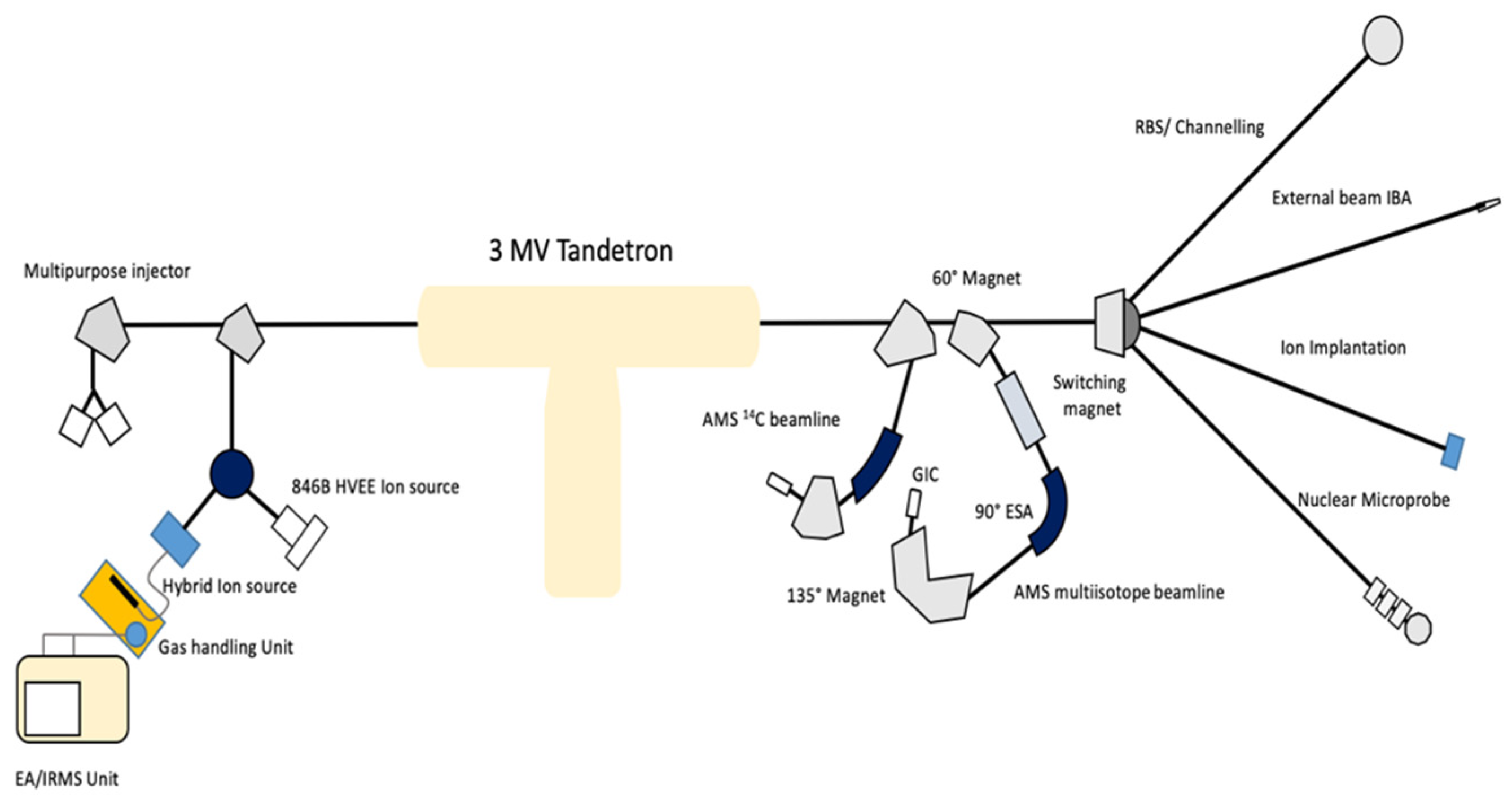
The term represents the ratio between the 14C and the 12C concentrations in the sample to be dated. The complexity of the experimental approaches needed to measure this term is related to the low natural abundance of 14C (in a modern sample the 14C/12C ratio is of the order of 10−12) which requires an extremely high sensitivity analytical technique. The technique which is today used for 14C detection is AMS (Accelerator Mass Spectrometry). The detailed description of this technique, introduced since 1977, is largely beyond the scope of this paper but we highlight here its main features [4,5,6]. An AMS spectrometer (Figure 2) can be described as formed by different functional units which are used to extract the carbon ions from a sample, to filter out unwanted elements and interfering particles, separates the different carbon isotopes, detect and count them [7].
This is typically achieved by using experimental approaches derived from nuclear spectroscopy techniques which are based on the use of electric and magnetic fields to analyse the ions depending on their electric charge and mass and high-resolution particle detectors. AMS is nowadays a mature technique allowing accurate and precise experimental determinations with uncertainty level of 0.2–0.3% on the 14C/12C ratio measurement (at least for samples younger than ~10,000) which corresponds to an absolute uncertainty on the measured age of ±25/30 years and sensitivity of the order of 10−15–10−16 [8]. In the last 10–15 years AMS instruments underwent important technological developments which resulted in the downscaling of the dimensions and complexity of the machines and new experimental approaches [9,10].
2.2. Sample Preparation
In the accelerator mass spectrometer negative carbon ions are extracted from the sample in an ion source. The typical ion sources used in AMS radiocarbon dating are sputtering source where a focused beam of heavy ions (typically Cesium at energies of few keV) is used to sputter away negative carbon ions from the surface of a cathode. It is then mandatory that the sample to be dated is chemically and physically processed in order to remove contaminations and convert it in a form suitable for the accelerator ion source, which is typically graphite or, less commonly, carbon dioxide. Chemically processing consists of different steps and procedures which strongly depends on the sample matrix [11]. Aim of these procedures is to select a suitable sub-fraction of the sample and remove any contaminants whose isotopic signature is different from the samples to be dated and can then alter the obtained ages. In marine sciences different matrixes are commonly submitted for 14C dating such as water, sea grass species, remains of marine animals but the most common ones are probably carbonates: coral skeletons, marine shells or marine concretions and bio-constructions. In this case the samples are typically hydrolyzed under vacuum to CO2 by using a strong acid (H3PO4 or HCl). The released CO2 is then cryogenically purified and either directly used for the AMS measurements in gas-accepting ion sources or catalytically reduced to graphite. In AMS sample processing it is of a paramount importance to keep under control any possible source of contamination associated with the chemical processing itself. This is typically ensured by processing, in parallel with the samples, standard reference materials with known ages and blank samples completely depleted in 14C. Nowadays the strict control of the employed procedures, the use of high purity chemicals and solvents result in blank levels of the order of 10−15 (as 14C/12C ratio) which allows to obtain reliable ages on samples as old as 45,000–48,000 years. Moreover, in sample preparation important improvements have been introduced in the last years which resulted in reduced processing times and new applications. This is for instance the case of the use of laser ablation for in situ sampling of carbonate records which allows rapid and spatially resolved 14C analyses [12].
3. Calibration of “Marine Ages”
Though simple in its basic principle the application of radiocarbon dating requires important aspects to be considered in order to obtain accurate and reliable age determinations. Indeed, one of the major issues is related to the variable 14C concentration in the Earth carbon pools over the millennia. As an important consequence, the term introduced in the radiocarbon decay law and indicating the 14C concentration in the considered reservoir at the time of death is not constant over the time. This is due to complex phenomena such as variations of the Earth magnetic field, of the solar activity and of the cosmic ray flux, to cite some of them. This means, in other words, that organisms which lived in different times up-took different levels of radiocarbon during their life. In order to obtain accurate age estimation, it is then fundamental to correct or “calibrate” for this effect. This can only be done by properly reconstructing the 14C concentration in the terrestrial atmosphere for the period of interest for 14C dating, essentially the last 50,000 years.
The curve representing the 14C concentration in the atmosphere is refereed as calibration curve and is obtained by measuring the 14C concentration in absolutely dated proxy records. Examples of these records are dendro-dated tree ring sequences, U/Th dated corals, laminated sedimentary sequences, speleothems. Figure 3 shows the 14C concentration reconstructed for the terrestrial atmosphere by the INTCAL20 working group [13].
In the figure the 14C concentration in the last 55,000 years shown in terms of Δ14C which represent the relative difference (in per mil and corrected for radiocarbon decay) between the 14C concentration in a given year and the reference value assumed in 1950 [15].
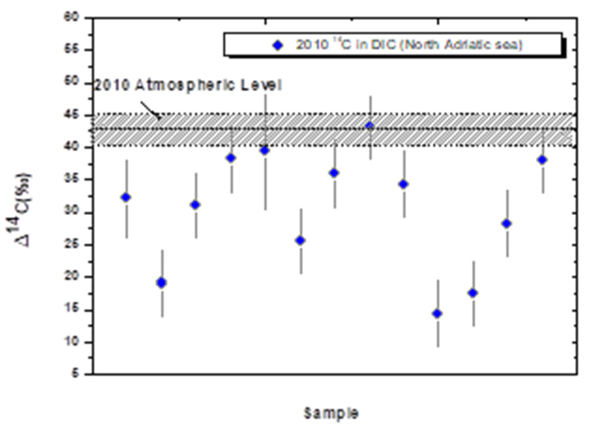
The calibration of radiocarbon ages obtained for sample fixing (radio)carbon from the sea and the ocean has to consider that surface-sea water is depleted in terms of 14C concentration when compared with the atmosphere. This can be seen in Figure 3 which shows that the 14C concentration in the marine pool is systematically lower than in the coeval atmosphere while high frequency fluctuations components are damped [14]. Figure 4 shows the comparison between the 14C concentration measured in the atmosphere [16] and in Dissolved Inorganic Carbon (DIC) extracted from shallow water sampled from the Northern Adriatic Sea in 2010 at depth ranging from 14 to 30 m [17]. It can be immediately seen that sea water is depleted in 14C concentration when compared with the atmosphere.
This Marine Reservoir Effect (MRE) has a profound impact on the dating of marine samples which show 14C ages apparently older than the real ones [18]. In order to correct for this effect, the depletion of the 14C concentration in sea-surface water is conventionally and quantitatively expressed by introducing the R (Marine Reservoir Age) term which can be defined as the difference between the 14C age obtained for a given marine sample Rmarine and the corresponding age of a coeval organism fixing carbon from the atmosphere (Rterrestrial):
It is worth noting that this difference essentially mirrors the difference between the 14C age in the atmospheric CO2 and the 14C age of the Dissolved Inorganic Carbon in the surface ocean water. Unfortunately, the R term is not constant across the globe and it is also function of time meaning that for the same location it can have different values at different times. In order consider, the local deviations of the R term from a global average a ΔR term is then introduced defined as:
where Rlocal and Raverage are the local and the global average marine reservoir effect. This term can be measured in different ways such as the dating of paired terrestrial and marine samples or the dating of marine samples of known age. The methodological approach used for the calibration of marine ages can be then very quickly summarized as follows. A “global” marine curve is constructed starting from the atmospheric one and by applying proper global cycle models [14]. The global marine curve internationally accepted is now called MARINE20 and it is derived from the INTCAL20 curve. They are both shown in Figure 3. This global curve is then “corrected” for local effects by applying the proper ΔR term for the particular location where a certain sample was living. This methodology allows the correction of radiocarbon marine ages though the most critical aspect is related to the knowledge of the proper ΔR term for the given location and the considered time. It is also important to underline that calibrated marine ages are typically affected by larger statistical errors than atmospheric ones due to the larger uncertainties associated with the marine curve and the error propagation on ΔR estimation. The accuracy of the obtained results largely depends on the proper estimation of the local reservoir effects. An example of the application of the described approach is shown in Figure 5. Let us assume that a marine shell was 14C dated to 1000 ± 35 BP and that the sample was taken from the Southern Adriatic Sea were a ΔR = −102 ± 30 has been measured and derived from the online 14CHRONO Marine reservoir database available at the address http://calib.org/marine/ accessed on 31 March 2021. The results of calibration are shown in Figure 5 as obtained by using the software OxCal Ver. 4.4 [19] and the MARINE20 database. The light red Gaussian curve indicates the probability distribution obtained for the sample (1000 ± 35 BP in our case). A distribution, corrected for the local deviation from the average, global curve is then obtained considering the selected ΔR value and, of course, its uncertainty. The offset dark red curve is then obtained. Its larger width (standard deviation) is the result of the combination of the uncertainty on the radiocarbon age determination and in the ΔR value.
This “corrected” value is then calibrated against the global marine curve (the blue curve in the Figure) to obtain the calibrated, calendar age with a probability distribution function shown in grey. The one (68.2% probability) and two (95.4%) standard deviation confidence intervals are then calculated as shown in the right end corner. The comparison (and the corresponding large difference) between the calibrated age of 532 ± 65 years before 1950AD and the uncalibrated one 1000 ± 35 clearly show the importance of applying the proper corrections when dealing with marine radiocarbon data.
4. Applications
AMS radiocarbon dating is a routine tool for the study of different aspects related to the “marine” environment where it is used for the assessment of an absolute timeframe in different areas spanning from marine biology and ecology to coastal geomorphology, climatic and ocean circulation studies and sedimentology to name few of them. We review here some of the studies performed in this field at CEDAD-University of Salento in the last twenty years of activity of the Centre.
4.1. Analysis of Marine Bio-Construction
In the marine environment, there are different examples of biogenic formations such as reef structures formed by the carbonate skeletal materials of different organisms [20,21,22,23,24]. These structures are typically suitable for 14C analysis considering that they form their skeletons by up-taking carbon from the surrounding sea where 14C is dissolved from the atmosphere. In the Mediterranean Sea the most diffused biogenic formation is the coralligenous, though a different type of biogenic formations was reported in 2003 in the “Lu Lampiune” submerged cave at Cape of Otranto, Mediterranean Sea.
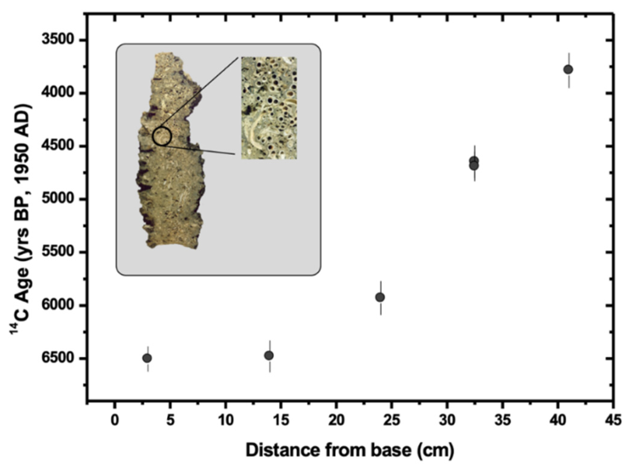
These biogenic formations, also refereed as pseudo-stalactites because of their shape, can be up to 2 m long, and show a core of Protula tubularia, calcareous tubes embedded and concealed in a fine brown-grey calcareous matrix of bacterial origin (Figure 6). These structures were deeply studied in the following years in order to identify their origin, describe their inner texture and propose a possible mechanism of formation. In these studies, the contribution of 14C dating was crucial because it allowed to define the timing of formation and evolution. Different radiocarbon dating campaigns were carried out by using as samples both the calcareous tubules and the microbial matrix. From the methodological point of view preliminary analyses of tubules produced by living organisms allowed to assess the possibility to use them as suitable samples for 14C dating. A 14C signal coherent with the expected level in the coeval sea was indeed obtained [25]. An example of the results obtained on samples extracted along the longitudinal axis of a sectioned stalactites is shown in Figure 6. It can be recognised that the age of the samples become younger as we move from the base to the tip of the stalactite along the longitudinal axis. The data show that the formation started ~6500 years ago when the cave was fully flooded and indirectly confirmed the fully submarine origin. The formation lasted ~three thousand years proceeding with a growth rate diminishing from the base to the top [26,27]. Similar results were obtained from different structures both by analysing the calcareous tube and by dating the matrix itself which revealed to be biogenic and resulted in a significant improvement in the understanding of the formation mechanism.
4.2. Sea Level Rise Studies
The study and the reconstruction of catastrophic coastal events such as storm waves or tsunamis [28] and sea-level variations, in particular during the Holocene, plays an important role in coastal geomorphology studies. This is in particular related to the general and growing concern about the impact of sea-level rise due to global warming on coastal communities, infrastructures and economical activities [29]. Indeed, sea-levels variations can be driven by both global and local phenomena. Global or eustatic phenomena are those related to variations of the global ocean mass or volume due to melting or accumulation of ice sheets at the North and South Poles. Local phenomena are related to glacio-hydro-isostatic and tectonic factors. The first ones are the results of the viscoelastic response of Earth due to the redistribution of ice and ocean weights while tectonic factors are associated with vertical movements such as uplift or subsidence due to tectonic forces [30]. Both local and global factors are in any case time-dependent and the accurate reconstruction of the complex patters of sea-level variations requires the use of suitable sea-level indicators whose age has to be constrained by proper absolute dating methods. Different sea-level indicators have been introduced and are routinely used which are divided in sedimentological, biological, erosional and archaeological categories each with its advantages, drawbacks and intrinsic accuracy [31]. Archaeological indicators include different kind of structures such as fish tanks, residential units, thermal baths, plumbing installations, quarries, beached wrecks just to name some of them [32]. Among the most commonly used biological indicators we mention vermetid reefs, cerastoderma glaucum, lithofaga which can be all dated by radiocarbon. Relevant results have been also obtained by using submerged speleothems, in particular sampled in cave environments. In this case radiocarbon dating is used to date different samples selected from different portion of the speleothems such as the last layer formed in aerial, continental conditions, the marine overgrowth encrusting the speleothem surface, or the so-called phreatic overgrowth formed in a brackish environment [33]. In sea-level rise studies the role of radiocarbon dating is, essentially, to give an absolute date to the different sea-level markers. Different aspects have to be properly addressed and deserve attention:
- The samples or sub-samples to be dated should be carefully identified and properly extracted from the matrix.
- Local marine reservoir correction factors should be used. This requires, when not available from literature data, its experimental estimation for instance through the measurement of paired terrestrial and marine samples from the same location or of marine samples with a known age.
- Possible local reservoir effects should be carefully evaluated, for instance those associated with 14C-depleted hard-water [34].
- Radiocarbon dates obtained on speleothems should be treated with caution and, when necessary, corrected for the possible contribution of 14C-depleted sources of carbon which can alter (making them older) 14C-ages. A detailed evaluation of the geological settings of the formation environment is mandatory as well as, when possible, paired U/Th analyses.
5. Conclusions
Accelerator Mass Spectrometry radiocarbon dating is a well-established absolute dating technique widely used in marine research. State-of-the art AMS spectrometers achieve routinely uncertainty levels of ±25/35 years, on sample younger than 10,000 years, and allow the analysis of organisms lived in the last 50,000 years. Nevertheless, specific issues have to be addressed when marine samples are submitted to 14C dating and mainly the need to use proper procedures in order to correct the obtained ages for the so-called marine reservoir age. We have described how this correction is carried out and the procedures which have to be used in order to obtain reliable and accurate marine ages. Though the extremely wide range of applications of 14C dating, we concentrated the present paper on the description of the analysis of marine bio-constructions and in the use of 14C in sea-level rise research.
Author Contributions
Conceptualization, writing, original draft preparation, writing—review and editing, G.Q.; resources and data curation, L.M.; methodology, M.D.; project administration and funding acquisition, L.C. All authors have read and agreed to the published version of the manuscript.
Funding
This research did not received external funding.
Institutional Review Board Statement
Not applicable.
Informed Consent Statement
Not applicable.
Data Availability Statement
No new data were created or analyzed in this study. Data sharing is not applicable to this article.
Conflicts of Interest
The authors declare no conflict of interest.
References
- Masarik, J.; Beer, J. Simulation of particle fluxes and cosmogenic nuclide production in the Earth’s atmosphere. J. Geophys. Res. Atmos. 1999, 104, 12099–12111. [Google Scholar] [CrossRef] [Green Version]
- Kutschera, W. The Half-Life of 14C—Why Is It So Long? Radiocarbon 2019, 61, 1135–1142. [Google Scholar] [CrossRef]
- Arnold, W.F.; Libby, W. Age determinations by radiocarbon content: Checks with samples of known age. Science 1949, 110, 678–680. [Google Scholar] [CrossRef] [PubMed]
- Bennett, C.L.; Beukens, R.P.; Clover, M.R.; Gove, H.E.; Liebert, R.B.; Litherland, A.E.; Purser, K.H.; Sondheim, W.E. Radiocarbon dating using electro-static accelerators. Science 1977, 198, 508–510. [Google Scholar] [CrossRef] [PubMed]
- Purser, K.H.; Liebert, R.B.; Litherland, A.E.; Benkens, R.P.; Gove, H.E.; Bennett, C.L.; Clover, M.R.; Sondheim, W.E. An attempt to detect stable N ions from a sputter ion source and some implications of the results for the design of tandems for ultra-sensitive carbon analysis. Rev. Phys. Appl. 1977, 12, 1487–1492. [Google Scholar] [CrossRef] [Green Version]
- Nelson, D.E.; Korteling, R.G.; Stott, W.R. Carbon-14: Direct detection at natural concentrations. Science 1977, 198, 507–508. [Google Scholar] [CrossRef] [PubMed]
- Calcagnile, L.; Quarta, G.; D’Elia, M. High resolution accelerator-based mass spectrometry: Precision, accuracy and background. Appl. Radiat. Isot. 2005, 62, 623–629. [Google Scholar] [CrossRef]
- Calcagnile, L.; Quarta, G.; D’Elia, M.; Gottdang, A.; Klein, M.; Mous, D.J.W. Radiocarbon precision tests at the Lecce AMS facility using a sequential injection system. Nucl. Instrum. Methods Phys. Res. Sect. B Beam Interact. Mater. At. 2004, 215, 561–564. [Google Scholar] [CrossRef]
- Synal, H.A.; Stocker, M.; Suter, M. MICADAS: A new compact radiocarbon AMS system. Nucl. Instrum. Methods Phys. Res. Sect. B Beam Interact. Mater. At. 2007, 259, 7–13. [Google Scholar] [CrossRef]
- Braione, E.; Maruccio, L.; Quarta, G.; D’Elia, M.; Calcagnile, L. A new system for the simultaneous measurement of δ13C and δ15N by IRMS and radiocarbon by AMS on gaseous samples: Design features and performances of the gas handling interface. Nucl. Instrum. Methods Phys. Res. Sect. B Beam Interact. Mater. At. 2015, 361, 387–391. [Google Scholar] [CrossRef]
- D’Elia, M.; Calcagnile, L.; Quarta, G.; Rizzo, A.; Sanapo, C.; Laudisa, M.; Toma, U.; Rizzo, A. Sample preparation and blank values at the AMS radiocarbon facility of the University of Lecce. Nucl. Instrum. Methods Phys. Res. Sect. B Beam Interact. Mater. At. 2004, 223–224, 278–283. [Google Scholar] [CrossRef]
- Welte, C.; Wacker, L.; Hattendorf, B.; Christl, M.; Koch, J.; Synal, H.; Günther, D. Novel Laser Ablation Sampling Device for the Rapid Radiocarbon Analysis of Carbonate Samples by Accelerator Mass Spectrometry. Radiocarbon 2016, 58, 419–435. [Google Scholar] [CrossRef]
- Reimer, P.; Austin, W.; Bard, E.; Bayliss, A.; Blackwell, P.; Bronk Ramsey, C.; Butzin, M.; Cheng, H.; Edwards, R.L.; Friedrich, M.; et al. The IntCal20 Northern Hemisphere Radiocarbon Age Calibration Curve (0–55 cal kBP). Radiocarbon 2020, 62, 725–757. [Google Scholar] [CrossRef]
- Heaton, T.; Köhler, P.; Butzin, M.; Bard, E.; Reimer, R.; Austin, W.; Skinner, L.; Ramsey, C.B.; Grootes, P.M.; Hughen, K.A.; et al. Marine20—The Marine Radiocarbon Age Calibration Curve (0–55,000 cal BP). Radiocarbon 2020, 62, 779–820. [Google Scholar] [CrossRef]
- Stuiver, M.; Polach, H.A. Discussion: Reporting of 14C data. Radiocarbon 1977, 19, 355–363. [Google Scholar] [CrossRef] [Green Version]
- Hammer, S.; Levin, I. Monthly mean atmospheric D14CO2 at Jungfraujoch and Schauinsland from 1986 to 2016. Tellus B 2017. [Google Scholar] [CrossRef]
- Macchia, M.; D’Elia, M.; Quarta, G.; Gaballo, V.; Braione, E.; Maruccio, L.; Calcagnile, L.; Ciceri, G.; Martinotti, V.; Wacker, L. Extraction of dissolved inorganic carbon (DIC) from seawater samples at CEDAD: Results of an intercomparison exercise on samples from Adriatic sea shallow water. Radiocarbon 2013, 55, 579–584. [Google Scholar] [CrossRef] [Green Version]
- Alves, E.Q.; Macario, K.; Ascough, P.; Bronk Ramsey, C. The worldwide marine radiocarbon reservoir effect: Definitions, mechanisms, and prospects. Rev. Geophys. 2018, 56, 278–305. [Google Scholar] [CrossRef]
- Bronk Ramsey, C. Development of the Radiocarbon Calibration Program. Radiocarbon 2001, 43, 355–363. [Google Scholar] [CrossRef] [Green Version]
- Ingrosso, G.; Abbiati, M.; Badalamenti, F.; Bavestrello, G.; Belmonte, G.; Cannas, R.; Benedetti-Cecchi, L.; Bertolino, M.; Bevilacqua, S.; Bianchi, C.N.; et al. Mediterranean Bioconstructions Along the Italian Coast. Adv. Mar. Biol. 2018, 79, 61–136. [Google Scholar] [PubMed]
- Guido, A.; Heindel, K.; Birgel, D.; Rosso, A.; Mastandrea, A.; Sanfilippo, R.; Russo, F.; Peckmann, J. Pendant bioconstructions cemented by microbial carbonate in submerged marine caves (Holocene, SE Sicily). Palaeogeogr. Palaeoclimatol. Palaeoecol. 2013, 388, 166–180. [Google Scholar] [CrossRef]
- Guido, A.; Gerovasileiou, V.; Russo, F.; Rosso, A.; Sanfilippo, R.; Voultsiadou, E.; Mastandrea, A. Composition and biostratinomy of sponge-rich biogenic crusts in submarine caves (Aegean Sea, Eastern Mediterranean). Palaeogeogr. Palaeoclimatol. Palaeoecol. 2019, 534, 109338. [Google Scholar] [CrossRef]
- Sanfilippo, R.; Rosso, A.; Guido, A.; Mastandrea, A.; Russo, F.; Riding, R.; Taddei Ruggiero, E. Metazoan/microbial biostalactites from modern submarine caves in the Mediterranean Sea. Mar. Ecol. 2015, 36, 1277–1293. [Google Scholar] [CrossRef]
- Rosso, A.; Sanfilippo, R.; Guido, A.; Gerovasileiou, V.; Taddei Ruggiero, E.; Belmonte, G. Coloniser of the dark: Biostalactite-associated metazoans from “lu Lampiùne” submarine cave (Apulia, Mediterranean Sea). Mar. Ecol. 2021, 42, e12634. [Google Scholar]
- D’Elia, M.; Quarta, G.; Calcagnile, L.; Belmonte, G. Study of the formation of biogenic speleothems found in submarine caves at the cape of Otranto, Italy, by 14C AMS. Nucl. Instrum. Methods Phys. Res. Sect. B Beam Interact. Mater. At. 2007, 259, 395–397. [Google Scholar] [CrossRef]
- Belmonte, G.; Ingrosso, G.; Poto, M.; Quarta, G.; D’Elia, M.; Onorato, R.; Calcagnile, L. Biogenic stalactites in submarine caves at the Cape of Otranto (SE Italy): Dating and hypothesis on their formation. Mar. Ecol. 2009, 30, 376–382. [Google Scholar] [CrossRef]
- Quarta, G.; D’Elia, M.; Calcagnile, L.; Belmonte, G.; Ingrosso, G. Reconstructing the formation mechanism of submarine biogenic stalactites: The contribution of AMS. Nucl. Instrum. Methods Phys. Res. Sect. B Beam Interact. Mater. At. 2010, 268, 1244–1247. [Google Scholar] [CrossRef]
- Pepe, F.; Corradino, M.; Parrino, N.; Besio, G.; Lo Presti, V.; Renda, P.; Calcagnile, L.; Quarta, G.; Sulli, A.; Antonioli, F. Boulder coastal deposits at Favignana Island rocky coast (Sicily, Italy): Litho-structural and hydrodynamic control. Geomorphology 2018, 303, 191–209. [Google Scholar] [CrossRef]
- Antonioli, F.; De Falco, G.; Lo Presti, V.; Moretti, L.; Scardino, G.; Anzidei, M.; Bonaldo, D.; Carniel, S.; Leoni, G.; Furlani, S.; et al. Relative Sea-Level Rise and Potential Submersion Risk for 2100 on 16 Coastal Plains of the Mediterranean Sea. Water 2020, 12, 2173. [Google Scholar] [CrossRef]
- Rovere, A.; Stocchi, P.; Vacchi, M. Eustatic and Relative Sea Level Changes. Curr. Clim. Chang. Rep. 2016, 2, 221–231. [Google Scholar] [CrossRef] [Green Version]
- Lambeck, K.; Antonioli, F.; Purcell, A.; Silenzi, S. Sea-level change along the Italian coast for the past 10,000 yr. Quat. Sci. Rev. 2004, 23, 1567–1598. [Google Scholar] [CrossRef]
- Auriemma, R.; Solinas, E. Archaeological remains as sea level change markers: A review. Quat. Int. 2009, 206, 134–146. [Google Scholar] [CrossRef]
- Antonioli, F.; Furlani, S.; Montagna, P.; Stocchi, P. The Use of Submerged Speleothems for Sea Level Studies in the Mediterranean Sea: A New Perspective Using Glacial Isostatic Adjustment (GIA). Geosciences 2021, 11, 77. [Google Scholar] [CrossRef]
- Quarta, G.; Fago, P.; Calcagnile, L.; Cipriano, G.; D’Elia, M.; Moretti, M.; Scardino, G.; Valenzano, E.; Mastronuzzi, G. 14C Age Offset in the Mar Piccolo Sea Basin in Taranto (Southern Italy) Estimated on Cerastoderma Glaucum (Poiret, 1789). Radiocarbon 2019, 61, 1387–1401. [Google Scholar] [CrossRef]
Figure 1.
Schematic representation of the mechanism underlying the uptake of carbon from marine organisms.
Figure 1.
Schematic representation of the mechanism underlying the uptake of carbon from marine organisms.
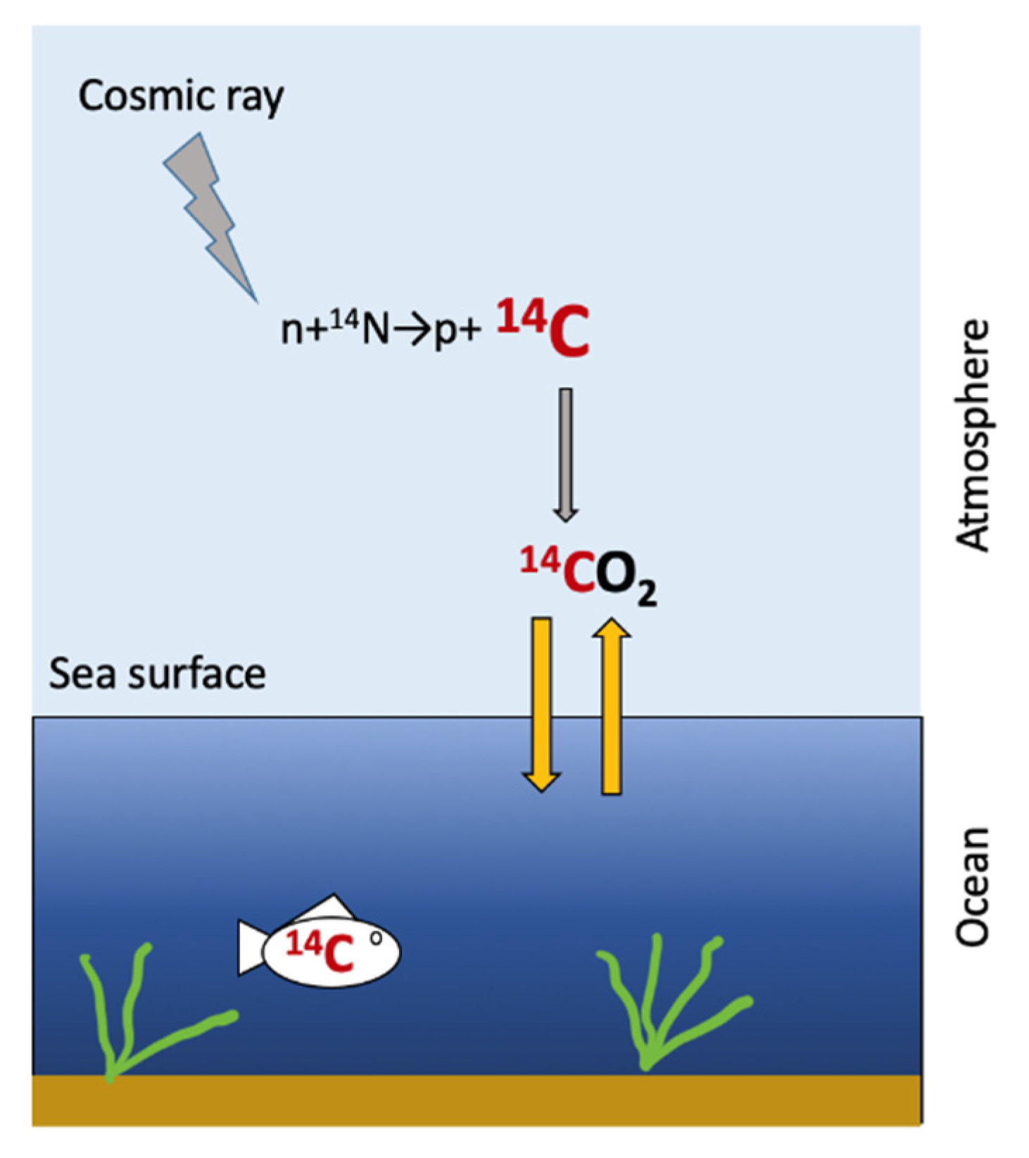
Figure 2.
Schematic of the accelerator-based facility at CEDAD-University of Salento. One of the six experimental beamlines is dedicated to 14C dating.
Figure 2.
Schematic of the accelerator-based facility at CEDAD-University of Salento. One of the six experimental beamlines is dedicated to 14C dating.

Figure 3.
14C concentration in the last 55,000 years in the terrestrial atmosphere (grey curve) and in the ocean (blue curve). The marine curve refers to the global average (see text for details). The curves are obtained by using the INTCAL20 [13] and MARINE20 [14] data records.
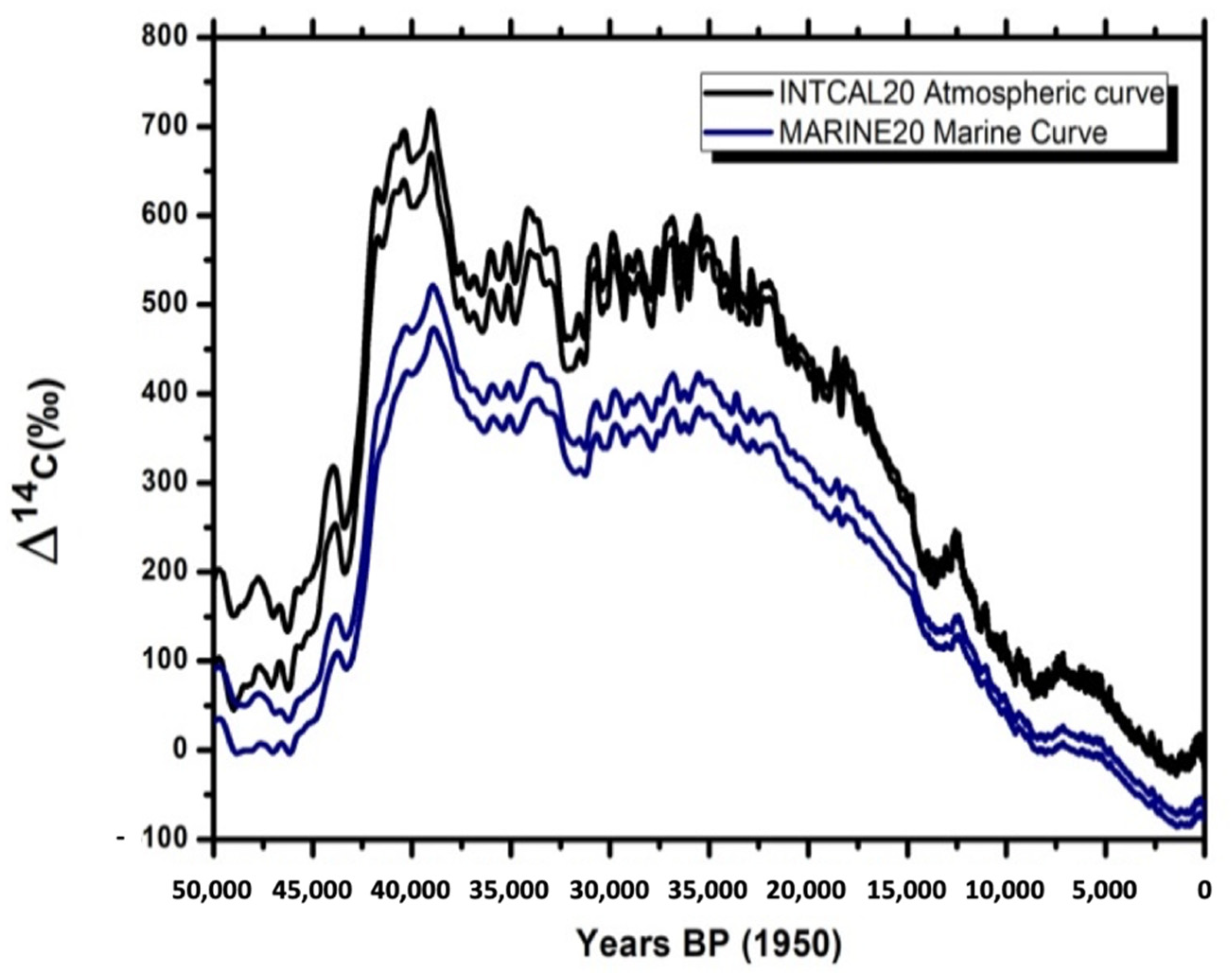
Figure 4.
Comparison between the 14C concentration measured in the 2010 atmosphere and in Dissolved Inorganic Carbon (DIC) extracted from sea water (North Adriatic Sea).
Figure 4.
Comparison between the 14C concentration measured in the 2010 atmosphere and in Dissolved Inorganic Carbon (DIC) extracted from sea water (North Adriatic Sea).

Figure 5.
Example of the calibration of a radiocarbon age for marine organisms having a conventional radiocarbon age of 1000 ± 35 years BP and hypothetically sampled in the Southern Adriatic Sea. The light red Gaussian curve indicates the probability distribution obtained for the sample (1000 ± 35 BP in our case). A distribution, corrected for the local deviation from the average, global curve is then obtained considering the selected ΔR value and, of course, its uncertainty. The offset dark red curve is then obtained.
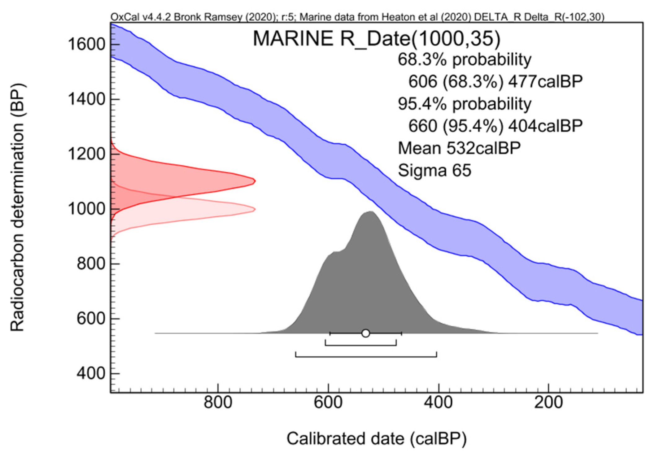
Figure 6.
One of the analysed bio-formations from “Lu Lampiune cave” with a closeup view of its inner texture. The graph shows the calibrated radiocarbon age for the sample taken along the longitudinal axis of the pseudo-stalactite as a function of the distance from the base.
Figure 6.
One of the analysed bio-formations from “Lu Lampiune cave” with a closeup view of its inner texture. The graph shows the calibrated radiocarbon age for the sample taken along the longitudinal axis of the pseudo-stalactite as a function of the distance from the base.
Publisher’s Note: MDPI stays neutral with regard to jurisdictional claims in published maps and institutional affiliations. |
© 2021 by the authors. Licensee MDPI, Basel, Switzerland. This article is an open access article distributed under the terms and conditions of the Creative Commons Attribution (CC BY) license (https://creativecommons.org/licenses/by/4.0/).
Share and Cite
MDPI and ACS Style
Quarta, G.; Maruccio, L.; D’Elia, M.; Calcagnile, L. Radiocarbon Dating of Marine Samples: Methodological Aspects, Applications and Case Studies. Water 2021, 13, 986. https://doi.org/10.3390/w13070986
AMA Style
Quarta G, Maruccio L, D’Elia M, Calcagnile L. Radiocarbon Dating of Marine Samples: Methodological Aspects, Applications and Case Studies. Water. 2021; 13(7):986. https://doi.org/10.3390/w13070986
Chicago/Turabian StyleQuarta, Gianluca, Lucio Maruccio, Marisa D’Elia, and Lucio Calcagnile. 2021. "Radiocarbon Dating of Marine Samples: Methodological Aspects, Applications and Case Studies" Water 13, no. 7: 986. https://doi.org/10.3390/w13070986
Note that from the first issue of 2016, this journal uses article numbers instead of page numbers. See further details here.