
A Review of Numerical Simulations of Secondary Flows in River Bends


1
Department of Civil Engineering, University of Ottawa, 161 Louis Pasteur, Ottawa, ON K1N 6N5, Canada
2
Department of Water Resources Engineering, Dalian University of Technology, Dalian 116024, China
*
Authors to whom correspondence should be addressed.
Water 2021, 13(7), 884; https://doi.org/10.3390/w13070884
Submission received: 21 February 2021
/
Revised: 15 March 2021
/
Accepted: 18 March 2021
/
Published: 24 March 2021
(This article belongs to the Special Issue Computational Fluid Mechanics and Hydraulics)
Abstract
:River bends are one of the common elements in most natural rivers, and secondary flow is one of the most important flow features in the bends. The secondary flow is perpendicular to the main flow and has a helical path moving towards the outer bank at the upper part of the river cross-section, and towards the inner bank at the lower part of the river cross-section. The secondary flow causes a redistribution in the main flow. Accordingly, this redistribution and sediment transport by the secondary flow may lead to the formation of a typical pattern of river bend profile. It is important to study and understand the flow pattern in order to predict the profile and the position of the bend in the river. However, there are a lack of comprehensive reviews on the advances in numerical modeling of bend secondary flow in the literature. Therefore, this study comprehensively reviews the fundamentals of secondary flow, the governing equations and boundary conditions for numerical simulations, and previous numerical studies on river bend flows. Most importantly, it reviews various numerical simulation strategies and performance of various turbulence models in simulating the flow in river bends and concludes that the main problem is finding the appropriate model for each case of turbulent flow. The present review summarizes the recent advances in numerical modeling of secondary flow and points out the key challenges, which can provide useful information for future studies.
1. Introduction
Rivers rarely run on straight paths, and most of them run on a curved route. The flow patterns on river bends are very complicated and have special characteristics. Basically, flow patterns in river bends are affected by certain factors such as the centrifugal force caused by the flow curvature and the vertically varying velocity, the cross-sectional stress, in addition to the pressure gradient in the radial direction due to the lateral slope of the water’s surface. All these factors create a flow called secondary flow (Ghobadian and Mohammadi, 2011) [1], which may significantly affect the primary flow motion and, in turn, affect pollutant dispersion and sediment transport. Therefore, it is important to predict and estimate the flow behavior of river bends for proper design of nearby hydraulic structures, environmental and ecological assessments, and sound planning of inhabitation projects.
Flow patterns and characteristics in river bends have been widely studied due to the major significance of this subject. The secondary flow, according to Rozovskii (1961) [2] and De Vriend (1979,1980) [3,4], is a helical path moving toward the outer bank at the upper part of the river and moving toward the inner bank at the lower part of the river. Thus, a slight deviation occurs on the shear force, which follows the same direction as the local flow near the bed. This deviation is from the direction of the mean flow (Engelund and Skovgaard, 1973) [5].
The flow in river bends can be studied using either physical or numerical methods. Several experimental and laboratory studies were performed to investigate the flow features in river bends (Blanckaert and Graf, 2001; Booij, 2003; Reinauer and Hager, 1997; Roca et al., 2007; Tominaga and Nagao, 2000) [6,7,8,9,10]. These studies aimed to collect data on flow variables in channel bends and analysis of the results. The parameters studied in the papers include the flow velocity components, the secondary flow cells including the outer bank cells, etc. These studies have provided the knowledge base for understanding bend flows. However, the requirements of cost and time for the physical tests motivated the researchers to discover more flexible and inexpensive tools to examine flow behavior, which is represented by the numerical models.
The accurate simulation of the flow in curved channels requires a 3D hydrodynamic model. The flow field in curved channels was simulated by several 3D models, which were developed by researchers such as De Vriend, 1980 [4]; Shimizu et al., 1990 [11]; Wang and Hu, 1990 [12]. In addition, two-dimensional (2D) models were applied by other researchers to simulate the flow in curved channels (Hsieh and Yang, 2003; Ikeda and Nishimura, 1986; Molls and Chaudhry, 1995) [13,14,15]. At straight channels, or when the effect of the curvature is small, the secondary flows are mainly produced by the non-homogeneity and anisotropy of turbulence (Wang and Cheng, 2006) [16], so there is no significant effect from the secondary flow in many practical cases.
According to Chang (1971) [17] and Fischer (1969) [18], the transverse mixing caused by the secondary flow in curved channels is much stronger than that in straight channels. Some researchers (Booij, 2003; Kang and Choi, 2006; Khosronejad et al., 2007) [7,19,20] indicated that there is a limited capability to predict the secondary flow by isotropic turbulence models such as the k-ɛ model. Thus, the study of flow around bends typically requires higher-order turbulence models such as Reynolds stress models (RSM) and large eddy simulation (LES) (Booij, 2003; Luo and Razinsky, 2009; van Balen et al., 2009) [7,21,22], especially when the bend of the channel is of a sharp type (Marriott, 1999; van Balen et al., 2009; Zeng et al., 2008) [22,23,24].
The distribution of helical flow strength and its changes along channels were first studied by Mosonyi and Gotz (1973) [25]. They showed that the strength changes of the secondary flow can well describe the flow itself. Additionally, the existence of the second cycle of the secondary flow near the internal bend, which happens only at the channel of (bed width/water depth) <10, was reported by them for the first time. The finite difference method was used by Leschziner and Rodi (1979) [26] to apply their three-dimensional numerical model to calculating flow in strongly curved open channels (180° bend with straight inlet and outlet reaches) with a rectangular cross-section. The standard k-ɛ model was employed in their study to produce the correct eddy–viscosity distribution in a wide range of flow situations. The transverse surface slope and velocity field in the curved channel were predicted and presented. The results obtained from the employed model were judged to be satisfactory for all major flow phenomena.
There is a lack of comprehensive reviews on the advances in numerical modeling of bend secondary flow in the literature. Therefore, this study aims to review some of the previous studies that used numerical models to simulate the secondary flow in river bends. The main motivation of this review is to assess these numerical models used in simulations and choose a suitable numerical model to simulate the behavior of the flow in the river bends from the researcher’s point of view. The main point of this review is to determine the choice of the model dimension (i.e., 2D or 3D), selection of a turbulent model (RANS, LES, etc.), and application in different channel geometries (single curved channel or meandering).
This paper is organized as follows: Section 2 deals with the secondary flow in river bends. Section 3 covers boundary conditions, and Section 4 reviews the numerical studies on river bends including different kinds of bends in different situations and some effects of secondary flows in these rivers. Section 5 is the discussion. Section 6 is the critical review and future research needs. Finally, the conclusions complete the study.
2. Secondary Flow in River Bends
2.1. Mechanism of Secondary Flow
Given the importance of secondary flow in river bends, and its significant effects on the main flow particularly, and on the bottom configuration of the river generally, it is important to study these effects in river bends and take them into consideration in the design of river engineering works. The secondary flow is a helical path moving towards the outer bank of the river in the upper part and towards the inner bank of the river in the lower part of the cross-section, as shown in Figure 1.
The main flow of the curved channel is affected by the redistribution of the velocity. The velocity increases near the outer bank of the channel and decreases near the inner bank of the channel (De Vriend, 1980) [4]. As the river enters the bend, the flow particles are affected by the acceleration due to centrifugal force. Accordingly, the flow particles tend to move towards the external wall of the river. Then, an increase in the water level occurs near the outside wall and decreases near the inside wall. Non-uniform pressure distribution is generated in the cross-section due to the slope of the free surface. This pressure increases near the external wall. Due to the difference between the small vertical accelerations and the high gravitational acceleration, there is a distribution of the hydrostatic pressure over the vertical. Subsequently, there is approximate equality in the pressure gradient in the radial direction over the vertical. Thus, the magnitude of the longitudinal velocities is equal at all points in the vertical direction and the centrifugal accelerations are completely counterbalanced by the centripetal acceleration. Due to the viscosity forces, there is a non-uniform distribution of the longitudinal velocity, which, in turn, causes a non-uniform distribution of the centrifugal acceleration. Accordingly, the velocity and the centrifugal acceleration increase near the flow surface and decrease near the bottom. The helical movement that is vertical to the main flow occurs because of the imbalance between the separate points in a vertical direction as shown in Figure 2. The movement of the helical path depends on the centrifugal acceleration, which means it is directed towards the outer bank at the upper part of the river as the centrifugal acceleration increases and towards the inner bank at the lower part of the river as the centrifugal acceleration decreases at this area. As the flow enters the bend, the free surface slope must be built up. Therefore, there is a negative pressure gradient near the internal wall and another positive pressure gradient close to the external wall (Jongbloed, 1996) [28].
At the exit of the bend, there is a positive pressure gradient near the interior wall and a negative one close to the exterior wall. The free surface slope decreases towards the bend exit until it may gradually become zero at the end of the bend.
2.2. Secondary Flow Cells
There are two regions that could be found in the bend of the curved channel: the center region cell and the outer bank cell. The center region cell is the classical helical or spiral motion of the secondary flow that moves toward the outer bank at the upper part of the river and moves toward the inner bank at the lower part of the river. The center region cell results from the interaction of the centrifugal force, the pressure gradient resulting from the inclined water level, and the roughness of the bed (Rozovskii, 1961) [2]. The outer bank cell is a counterrotating eddy at the outer bank of the channel (Bathurst et al., 1977) [29]. The outer bank cell is mainly caused by turbulence anisotropy and is a key feature of bend flow, and it has been found that the proximity of the water surface and the outer bank can affect its generation and characteristics (Blanckaert, 2009; Blanckaert, 2011) [30,31]. The outer bank cell is usually smaller and weaker than the center region cell. However, it should not be underestimated because it could be strongest in the sharp channel bends, and it has a stabilizing effect on the erosion of the outer bank and the mixing abilities in this region (Graf and Blanckaert, 2002) [32]. This is shown in Figure 3.
2.3. Velocity Redistribution
The flow distribution is nearly symmetric in straight channels, but the main velocity of the flow in channel bends is significantly affected by the secondary flow, and accordingly, a considerable redistribution occurs with respect to the main velocity. The flow particles that are close to the free surface are transported towards the outer bank of the river affected by the secondary flow. The core of the high-velocity region is near the inner bend at the bend entrance due to the potential vortex effect (Zeng et al., 2008) [24] and gradually shifts towards the outer bank due to secondary flow caused by the combined effects of pressure gradients and centrifugal forces. The velocity and momentum of these particles are larger compared to the ones in the outer bank. Thus, an increase occurs in the velocity of the outer bank region. The process is just the opposite near the bed of the river, where the flow particles with smaller velocity and momentum move towards the inner bank of the river, causing a low velocity at this area. The vertical convective transport of main flow momentum is significant at the area close to the sidewalls, while it is almost negligible near the central part of the river. The main reason for the velocity increase near the outer bank and reduction near the inner bank is vertical convection, while outward lateral interaction is due to radial convection (Jongbloed, 1996) [28]. The effect of secondary flow on the main flow is explained in Figure 4, where the streamlines represent the secondary flow and the isovels represent the main flow velocity.
Figure 4 presented above shows that the variance of velocities along the streamlines of the secondary flow near the bed of the river is not significant. The difference increases towards the inner bank, and then streamlines are almost vertical to the isovels near the surface of the river. There are some factors that affect the secondary flow, such as the distance between the isovels (the local main velocity gradient), the secondary flow strength, and the sine of the angle of intersection between the main flow isovels and the streamlines of the secondary flow. Note that the effect of the secondary flow in the wall district will be comparatively stronger in the upper part of the section where the velocity gradient is of the same order of magnitude throughout the vertical. As a result, the main velocity profile becomes flatter near the surface, which is confirmed by experimental research (Jongbloed, 1996) [28].
On the other hand, the longitudinal velocity component at the entry of a bend and in the early part of the internal wall area increases, accompanied by a steep fall of the free surface. In addition, extreme velocity is found at the free surface at this place in the cross-section (Booij and Tukker, 1996) [33]. It is noticed that the maximum velocity at the end of a 180° curved bend shifts outward—the outer part of the cross-section—due to the redistribution of the main velocity (De Vriend, 1980) [4], while the opposite situation is found at the outside wall area at the entry of a bend. Note that the longitudinal velocities decrease due to a positive pressure gradient.
2.4. Mathematical Description of the Main Flow and Secondary Circulation
The differential equations, which include the continuity equation and Reynolds-Averaged Navier–Stokes system, can be used to describe the three-dimensional incompressible fluid flow. For uniformity, these equations can be rewritten as below:
Conservation of mass:
The momentum equations:
where is the velocity vector; is the density; is the gravity acceleration; p is the pressure; T is the viscous stress tensor.
3. Boundary Conditions
The previous section introduced the mechanisms of secondary flow, the secondary flow cells, the velocity redistribution, and the governing equations. To simulate bend flows, certain boundary conditions should be applied, and the present section introduces the typical boundary condition setup.
There are four main kinds of boundaries for the numerical models that should be considered, namely: walls, free surface, inlet, and outlet.
3.1. Wall Boundaries
As the velocities at the wall are equal to zero and have large gradients in the vicinity, a very small grid distance should be used at this position. Thus, the high-Reynolds number model is no longer viable, and therefore, the first grid-point is defined at some distance from the wall (Jongbloed, 1996) [28]. Considering the effect of the viscous shear stresses or the turbulent shear stresses or both, it is recommended to separate the near-wall area into three regions (Booij, 1992) [34]: wall region, buffer layer region, and the turbulent boundary layer. At the wall region, the turbulent shear stresses can be abandoned (the so-called viscous sublayer). A buffer layer region comes next to the wall region where neither of the viscous shear stresses nor the turbulent shear stresses can be abandoned. The third region, the turbulent boundary layer, is distinguished where the viscous shear stresses can be abandoned. Accordingly, the boundary conditions and the first grid point should preferably be positioned in the last zones (Pezzinga, 1990) [35]. The boundary conditions for k (turbulent kinetic energy) and (turbulent energy dissipation rate) can be found using the following equations (Jongbloed, 1996) [27]:
where is shear velocity, is a model constant (0.09), and y is the distance to the wall.
Flow variation properties at the area close to the solid walls and bed are steep. To simulate the wall effect and estimate the turbulence parameters at this area, the wall function method is employed (Rodi, 1984) [36]. With the wall function, a fairly coarse grid is used in the area close to the wall. It is also considered to be an economical method of turbulent flow modeling (Jian and McCorquadale, 1998) [37]. Below are some of the turbulence equations for some models that use the wall function approach (Wilcox, 1998) [38]:
where = distance from the solid boundary to the center of the closest element; = turbulence kinetic energy at the closest cell to the wall; and = defined as follows:
where and = 11.53 (Melaaen, 1990) [39] and E is related to the roughness Reynold number as follows (Wu et al., 2000) [40]:
where equivalent roughness height of bed; B = additive constant = 5.2; = roughness function of the roughness Reynold number, which is calculated by (Cebeci and Bradshaw, 1977) [41]:
The equivalent roughness height quantified the influence of roughness elements.
3.2. Free Surface
For bend flow, the rigid-lid approximation is often adopted. The rigid-lid approximation is used when the Froude number is small, and a frictionless flat plane is assumed (Leschziner and Rodi, 1979) [26]. This approximation for this fictitious rigid lid does not neglect the changes in surface elevation but these changes are taken into account in an indirect manner. Accordingly, non-zero pressure gradients in the radial and vertical directions are expected at the boundary, which would result in some errors because the superelevated regions are implicitly considered hydrodynamically passive. However, experiments conducted by Mcguirk and Rodi (1977) [42] showed that the error associated with this approximation does not exceed approximately 10% of the total channel depth (Mcguirk and Rodi, 1977) [42]. Therefore, the following assumptions at the free surface can be formulated (Jongbloed, 1996) [28]:
- Vertical velocities are zero;
- The derivative in the vertical direction of the radial and longitudinal velocities are zero.
On the water surface, in absence of wind, the boundary conditions for the turbulence parameters are:
For the free surface, the turbulent kinetic energy and net fluxes of horizontal momentum are set as zero. The pressure normal to the surface is set to atmospheric, velocity is set to zero, and the dissipation rate is calculated from the relation given by (Rodi, 1993) [43]:
where h = local water depth.
3.3. Inlet
Determining the distributions of velocities and the parameters of the turbulence across the boundary of the inlet is likely not possible in practice. Therefore, most of these distributions are estimated based on physical reasoning. The experimental distribution of is rarely available and the -distribution can only be obtained indirectly from measurements of other turbulent quantities (Leschziner and Rodi, 1979) [26]. To smooth out the boundary conditions from the positions of interest, the boundaries must lie at a distance long enough for the flow if the errors caused by the assumptions for the boundary conditions cannot be neglected (Jongbloed, 1996) [28]. Below are some of the turbulence equations for some models that are used at the inlet:
where = inlet turbulent kinetic energy; = inlet turbulent kinetic dissipation rate; = average inlet velocity; = intensity of turbulence; and and = characteristic length of channel and length scale of the flow field, respectively.
3.4. Outlet
The discussion in the previous section can be used to determine the outlet boundary conditions. If the outlet boundary is far enough away, a zero gradient boundary condition may be employed for most variables.
4. Advantages and Disadvantages of Various Numerical Methods
Examples of the widely used turbulence modeling approaches include direct numerical simulation (DNS), Reynolds-averaged numerical simulation (RANS), RSM (Reynolds Stress Model), large eddy simulation (LES), and detached eddy simulation (DES). DNS is the most reliable approach, but its computational costs are super high and are, thus, not further discussed in this paper. The other turbulence modeling approaches are discussed in the present section.
4.1. RANS Modeling
For RANS models, the standard k−ε turbulence model (Versteeg and Malalasekera, 2007) [44] is considered to be relatively simpler. A very good performance can be achieved from the k-ε model in many cases as the model is well established. The model has also been extensively validated. However, it is considered more expensive than some other turbulence models, such as the mixing length model. The performance of the k-ε model may not be satisfactory in some cases, such as unconfined flows, flows with large extra strains, rotating flows, and flows driven by the anisotropy of normal Reynolds stresses.
The realizable k-ε model has been found to be more precise than some other models (e.g., the standard k-ε model) in predicting flows such as discrete flows and flows with complicated secondary flow features (Gildeh, 2013) [45].
The blending function drives the standard k−ω model in close wall regions and drives the k-ε family models in areas further from the surface. These differences make the SST model more accurate for a greater variety of flows than the standard k-ω model (Menter, 1994) [46].
4.2. RSM Modeling
RSM models may be considered as a subcategory of RANS models while they are computationally more expensive. According to Davidson (2011) [47], the advantages of RSMs could be summarized as follows: (1) the ability of RSM to respond effectively to any sudden change in the main strain; (2) modelling is not necessarily required for the production terms, which are used to explain many phenomena; and (3) the transport equations, which contain the main physical mechanisms that derive the evolution of turbulence such as production, redistribution, turbulent transport, viscous diffusion, and dissipation, are solved without assuming any behavior for Reynolds stresses. However, implementing the RSMs is considered to be a challenging task due to their complexity and CPU time consumption. Additionally, the numerical analyses of RSMs are very sensitive to influencing factors because of the small stabilizing of the second order derivatives of the momentum equations.
4.3. LES Modeling
Compared with the two-equation turbulence models (e.g., k-ε, k-ω), LES is typically more expensive in terms of computational costs. However, when comparing the computational cost with the accuracy of LES models, its efficiency, and other features with regard to computational time, can also be reasonable and worthy. This type of turbulence model can be more universally used since it overcomes the issues associated with using small eddies, such as tending to be more isotropic and less dependent on geometry. However, it is more computationally expensive since it needs finer grid densities for LES models than most RANS models. Although the large CPU costs for high-Re flows can be reduced by using a coarse near-wall mesh coupled with wall functions, the discretization schemes should be carefully designed to obtain more accurate results (Cable, 2009) [48].
4.4. DES Modeling
The DES model is a cross between the LES and RANS approaches. It is quite beneficial to combine the RANS modeling approach with the LES approach if the usage of LES models is computationally unaffordable. Typically, the DES method is much less expensive than the LES approach but more expensive than the RANS. In regions where large turbulence scales play a dominant role, the LES model based on the sub-grid model by the DES model is used. In areas where viscous impacts predominate, such as near-wall areas, the RANS model is used (Shur et al., 1999) [49].
5. Research on River Bends Flows and Key Findings
The previous sections have introduced the fundamentals of secondary flow, governing equations, and boundary conditions. Previous researchers have conducted numerical studies on river bend flows based on these fundamentals and configurations. This section reviews and discusses some of these studies and their key findings. The reviewed papers were mainly selected based on their research focuses, and they are classified into four categories: secondary flow in the curved channel; secondary flow and pollutant dispersion; secondary flow and sediment transport; and secondary flow in bend over topography.
5.1. Secondary Flow in a Curved Channel
In this section, some previous numerical research studies on secondary flow in channel bends were discussed, taking into account different bend geometries, and different models of turbulence. Then, each numerical model was examined and evaluated. Table 1 summarizes these numerical research studies and their key findings.
The standard k-ɛ model and the low-Reynolds number k-ω model were used by Khosronejad et al. (2007) [20] to simulate the flow in a channel bend. To validate the hydrodynamic model results, the experimental data of Ghanmi (1999) [57] were used. In this experiment, an S-shaped flume with two identical 90° reverse bends connected by a straight channel segment was used. The geometric parameters of the flume include the length of the straight channel segment (3.5 m), the rectangular channel cross-section (0.5 m wide and 0.4 m depth), and the inner radius of each channel bend ( = 1.25 m). The characteristics and flow conditions considered in the experiment were as follows: the channel boundary was made with aluminum covered with a sand layer with a median diameter, , of 2 mm, the discharge was 0.023 m3/s, the flow depth was h = 0.15 m, the mean inflow velocity was U = 0.3 m/s, and 2D velocities (longitudinal and transverse) were measured with a laser Doppler anemometer at 20 flume sections. The boundary conditions applied in this analysis included: inlet, outlet, free surface, and wall. At each section, three verticals were measured with five points for each vertical as shown in Figure 5. The results showed that the supreme velocity at the bend happens near the inner bank and moves toward the opposite bank as the outlet of the bend is approached. The streamwise velocity component differs from zero at or close to the bed to a maximum value when approaching the water surface. This situation is expected because it represents frictional effects. Based on the previous point, it can be intuitively concluded that the centrifugal force is greatest near the water surface and decreases with depth. The flow vectors near the bed are directed towards the inner bank and at the free surface towards the outer bank. The analysis showed that the mean absolute errors of the k-ω model (10.4%) are lower than the k-ɛ model (12.6%) in simulating the transverse velocities. Although the difference is relatively low, it could be concluded that the k-ω model is better than the k-ɛ model in simulating the transverse velocities which form the secondary flow phenomenon (Falcon 1984) [58].
The experiment of De Vriend (1979) [3] was used by Duan (2004) [50] to simulate the flow in a mildly curved channel. The channel comprised a 1.7-m-wide flume having a U-shaped ground plan, with vertical sidewalls and horizontal bottom. The radius of curvature of the flume axis in the bend was 4.25 m, and the length of both straight upstream and downstream was about 6.0 m. The ratio of radius of curvature to channel width was 3.5. The discharge at the inlet was 0.0671 m3/s, the averaged velocity was 0.202 m/s, and the averaged flow depth was 0.1953 m. The boundary condition of the upstream was the inflow unit discharge, and for the downstream was the measured flow depth. By including the dispersion terms, a depth-averaged 2D numerical model was used to simulate the flow in this curved flume, taking into account that various sets of longitudinal and secondary flow profiles for governing equations in Cartesian coordinates were used to derive the dispersion terms. The simulated velocity vector field using a 2D numerical model and surface elevation in shaded color are shown in Figure 6. As can be observed in this figure, the higher velocity is directed towards the inner bank of the bend, while the lower velocity is directed towards the outer bank of the bend. The main reason behind the increase in velocity at the inner bank is the transverse convection of momentum induced by the secondary flow. However, the effect of the secondary flow in the mild bend is very weak because the radius of channel curvature is much larger than the width of the channel. Furthermore, in the bend, the surface water level increases at the outer bank and decreases at the inner bank. The centrifugal force is the main reason behind the increased flow at the outer bank. Generally, there was an agreement between the simulated and measured surface elevations at the inner, outer bank, and the centerline (Duan, 2004) [50].
The experiment of Rozovskii (1961) [2] was used by Duan (2004) [50] to apply the depth-averaged 2D numerical model by including the dispersion terms 2D numerical model in a sharply curved open channel. It consisted of a 180° curved reach with a 6-m-long straight approach and a 3-m-long straight exit. The ratio of mean radius of curvature to width was 1.0. The width of the channel was 1.7 m. The cross-section of the channel was rectangular. Water depth at the downstream end was 0.053 m, and the discharge was 0.0123 m3/s. The surface elevation and velocity distribution are shown in Figure 7 below. There is an acceleration in the longitudinal flow close to the outer bank of the upstream part of the bend and a deceleration in the flow velocity near the outer bank. The surface elevation increased at the outer bank and decreased at the inner bank. There was good agreement between the simulated and measured results. The impact of secondary flow was observed on the depth-averaged flow distribution and water surface elevations, which became more visible with the increasing of the channel curvature. Due to the transverse bed slope in natural rivers, the velocity of secondary flow near the bed is higher. There is a significant role of the secondary flow in transporting bedload and suspended load in the transverse direction (Duan et al., 2001) [59]. Obviously, a 3D model is more accurate than that of a depth-averaged model. However, the depth-averaged two-dimensional model with the dispersion terms according to this study was capable of simulating the hydrodynamic flow in meandering channels. As the secondary flow could not be taken into account in the depth-averaged turbulence model, the Schmidt number that correlates mass dispersion with turbulent diffusion can be adjusted as a calibration parameter. Finally, the accuracy of the 2D approach is still limited according to the results, and more measurements for calibration and verification are needed to obtain more accurate results.
The channel of a 90° bend was used by Ghaneeizad et al. (2010) [51] to study the flow in a curved channel. The width of this channel was 0.4 m, the discharge was 13.55 lit/s, and the depth was 9 cm. The flow is subcritical, and the velocity on subcritical flows is at a high range. The boundary conditions were as follows: pressure-inlet, pressure-outlet, symmetry, and wall for the inlet, outlet, upper surface, and channel wall, respectively. Some turbulence models are used to simulate the flow in this channel including k-ω, k-ε (realizable), k-ɛ (RNG), and LES. Then, the simulated results are compared with the measured ones, and the ability of each model is examined with respect to flow analysis. Accordingly, the k-ε (RNG) model showed good performance in simulating the flow in the bend, and k- ω and k-ε (realizable) did not noticeably differ from the k-ε (RNG) model. However, LES has not shown its capability in simulating the flow in channel bends, especially after the curve (Ghaneeizad et al., 2010) [51].
The same channel of a 90° bend used by Ghaneeizad et al. (2010) [51] was also used by Gholami et al. (2014) [52] to study the flow patterns in a strongly curved open channel bend via the k-ɛ (RNG) model to predict the turbulence, and the volume of fluid (VOF) method to simulate the water’s free surface. The channel is shown in Figure 8 below. The inlet-water boundary was set as a velocity inlet. The free surface boundary was set as the pressure-inlet condition on which atmospheric pressure was assumed. The boundary at the downstream outlet was defined as a pressure-outlet condition, and wall functions were used to estimate the effect of walls. The water surface is uniform before and after the bend, while along the bend and because of the centrifugal force, a transversal slope occurs on the water’s surface. The higher velocity appeared near the inner bank along the bend while the lower velocity appeared near the outer bank. This pattern was reversed after the bend. The results of the comparison between the numerical model and the experimental data indicated that there is an acceptable level of agreement. Major secondary flows and minor ones (near the water surface and in the outer wall) with two opposite rotation directions are formed in the numerical model. The flow pattern is impacted by these two secondary flows, which stay after the bend of the channel for some distance. As the flow in the bend is affected by secondary flows, the velocity increases accordingly in the area close to the bed, more than that near the water surface. Additionally, the higher velocity depth gradations cause an increase in the shear stress.
The flume data by Siebert (1982) [60] were used by Stoesser et al. (2010) [53] to simulate the flow in meandering open channels by using steady Reynolds-Averaged Navier–Stokes equations (RANS) using an isotropic turbulence closure, and Large Eddy Simulation (LES). The Reynolds stress term was modeled by the standard k-ɛ turbulence model or by the standard k-ω turbulence model, respectively. The flume consisted of two successive 180° bends joined by a 0.5 m-long straight cross-over section. There was a 4 m-long straight inlet before the first bend and a 2 m-long outlet. The channel’s section was a rectangle of 0.25 m in width. For the boundary conditions, the mass-flux was kept constant to obtain a pressure gradient between the upstream and downstream sections of the domain. For the bed and side walls, a smooth boundary with the no-slip condition was used, and for the water’s surface, a fixed rigid lid with zero gradients for all variables was used. The results showed that the higher momentum moves from the inner bank of the channel at the entrance of the bend towards the outer bank near the bend exit. Both the LES and the RANS calculations agreed well with the measurements and there is no significant difference between them. The higher velocity appears near the inner bank of the channel at the beginning of the bend, and then it moves towards the outer bank due to the centripetal forces acting in the previous bend. The maximum velocity is predicted well by the LES under the free surface. Additionally, the moving of higher velocity towards the inner bank of the channel at the beginning of the bend is predicted well by both RANS simulations. However, the suppression of the maximum streamwise velocity below the water surface is absent. Both RANS simulation and the LES model agreed well with the experiment in predicting the primary cell and an outer bank secondary cell at the peak of the bend. However, the RANS code failed to predict the persistence of the outer bank cell until the exit of the bend. The results also showed a good agreement between RANS and LES in the comparison of the computed bed and side-wall shear stresses.
The same flume data by Siebert (1982) [60] were also used by Fraga et al. (2012) [54] to simulate the flow in open channel bends. Two types of models were used in this simulation to solve the unsteady Reynolds-Averaged Navier–Stokes equations (RANS). The first one was an isotropic turbulence closure (standard k-ε model), and the second one was a non-linear k-ε model which takes into account anisotropic effects. The boundary conditions were considered as: open boundaries, wall and free surface. The results were compared with the LES data from Stoesser et al. (2010) [53] who used the same flume to simulate the flow by using the steady Reynolds-Averaged Navier–Stokes equations (RANS) with an isotropic turbulence closure, and Large Eddy Simulation (LES). Both models were similar to the LES model, which showed the shift of high-energy momentum from the inner bank to the outer bank. The flow moved under the effect of centripetal forces towards the outer wall and momentum was concentrated there at the first bend. As the flow reaches the second bend, the higher momentum is still under the impact of centripetal forces and moving towards the inner bank, which represents the outer bank of the first bend. Then, along the second bend, the higher momentum moves towards the outer bank of the channel due to the centripetal forces. The streamwise velocity is affected by the secondary flow as well. The highest streamwise velocity is located at some depth under the free surface instead of on the surface itself. The higher primary velocity is located at some depth under the free surfaces of the outer bank because of the centripetal forces. All three models are in agreement regarding the typical features of meandering channels. Additionally, all three models showed that the counter-clockwise secondary cell was inherited from the first bend, while only the non-linear k-ε and LES models showed the counter-rotating secondary cell of the previous bend, which is coincident with the higher primary velocities. However, the non-linear k-ε model’s main secondary cell shape clearly differentiates it from the LES model.
The channel of Rozovskii (1961) [2] was used by Shaheed et al. (2018) [55] to simulate the flow in a closed curved channel. It consisted of a straight approach channel with a length of 6 m followed by a 180° bend with a mean radius of 0.8 m and an outlet section of 3 m. The channel cross-section was a 0.8 m-wide rectangle as shown in Figure 9 below.
Four boundary conditions were applied in this case that include: the inlet and the outlet of the channel, the walls (including side walls and bottom), and the surface of the channel (symmetry). The simulation was performed using the OpenFOAM model and pisoFoam solver, mostly used for incompressible and turbulent flows in closed channel cases (also referred to as the Rigid-lid Model, or RLM). Two turbulence models were used to perform the simulation of flow in closed river bends: the standard k–ε model and the realizable k–ε model. The distribution of the velocity is shown in the figure below. The velocity increases near the inner bank at the beginning of the bend, and then moves towards the outer bank at the end of the bend (Figure 10).
In order to examine the flow velocity, cross-sections were taken in the bend as shown in Figure 11. The comparison between the experimental data and the two models is shown in the figure, where: U is the depth-averaged velocity magnitude; and , , and are the longitudinal, vertical, and lateral velocity averaged over the depth, respectively. Note that the depth-averaged velocity is represented by the vertical axis and is non-dimensionalized by , which is the downstream mean velocity. The horizontal axis represents the radial distance , non-dimensionalized by the channel width, where B is the channel width and r and are the radius of curvature for the outer and inner banks, respectively. Both models performed well in the flow simulation of the bend. In addition, the comparison in the figure showed that the two models performed well compared to other numerical models that were used by other researchers. However, near the bend exit, there is a slight variation in the two models, particularly at the inner bank, due to the change from a curved to a straight channel, which makes the flow features in this region complex and not easy to capture, showing the weaknesses of the two models in this area (Shaheed et al., 2018) [55].
Different kinds of RANS turbulence models including standard k-ε, Re-Normalization Group (RNG) k-ε, realizable k-ε, k-ω, and shear stress transport (SST) k − ω were used by Yan et al. (2020) [56] to simulate the flow in a high-curvature 135° channel bend with an assessment of side slopes and its effects on the secondary flows. The channel was rectangular, and it included a straight inlet section of 12.19 m followed by a 135° bend and then a straight exit section of 2.44 m. The width was 1 m, and the height was 0.9 m with vertical acrylic walls. The performances of different turbulence models were compared against experimental measurements, and the best performing model was used to perform additional computations to assess the impact of different side slopes on the flow distribution. In addition to the velocity profiles, the models were also compared with more details in terms of the streamlines of secondary flow at the section 60° from the bend. Two circulation cells appeared in the observations—the main, bigger one that was rotating clockwise, and the smaller one that was rotating counterclockwise, which was also called the outer bank cell. The realizable k-ε model was found to be the best among the tested models, especially in capturing some small flow features, such as the outer bank cells.
There are other numerical simulation models in river bends that have been used in previous research studies. The effect of secondary flow on depth-averaged equations using a stress diffusion matrix was studied by Lien et al. (1999) [61]. They used a 180° bend with a rigid bed to examine the flow pattern using a two-dimensional numerical model. Accordingly, the effect of secondary flow on the maximum velocity path along the channel was indicated.
LES and RANS (k-ε model) were used by Booij (2003) [7] to simulate the flow pattern in a mild 180° bend with a rectangular section and rotating annular flumes. He concluded that the main characteristics of secondary flow and main flow could be produced by RANS computations. However, there were no satisfactory reproductions of the complicated secondary flow fields that could be given by RANS for the flow in rotating annular flumes and river bends. The secondary and main flow were reproduced well by LES for the mildly curved river. The turbulence was reproduced reasonably by LES and there was a low level of deviations in the computed secondary flow pattern of the rotating annular flume from the measured flow pattern. Additionally, the outer bank cell was reproduced well by the LES computations, unlike the RANS computations. LES computations had a small sensitivity towards the exact choice of modeling parameters.
Three types of turbulence models, including standard k-ε, k-ω and RSM, were used to model the flow pattern in a 180° bend by Safarzadeh Gandoshmin and Salehi Neishbouri (2005) [62]. They found that the flow pattern could be predicted reasonably by all three models within the direct channel. However, during the curve, the prediction of RSM was superior. In addition, the k-ω model could predict the rotation and the separation effect of flow more precisely than the standard k-ɛ model.
The currents and mass transport in curved channels were simulated via a 3D hydrodynamic model of free surface turbulent flows by Jian and McCorquadale (1998) [37]. They modified the standard k-ɛ model and applied it to two typical curved open channel flows: a 270° channel bend with a sloped outer bank and a meandering channel with mass transport. Then, they compared the model results with available data and obtained generally good agreement. According to their simulation, the secondary flows of the single bend were much stronger than that of the meanders. The reason might be related to the opposite spiral movement generated by the alternate bends of the meandering channels. Additionally, there could be a large lateral mass transport in the curved channel because of the secondary flows.
A 3D numerical model was applied by Lu et al. (2004) [63] to simulate the flow pattern in a channel with a 180° bend using the standard k-ɛ turbulence model. The results of the comparison between the numerical model and experimental data showed acceptable agreement. However, the model was not able to predict the minor secondary rotational cell in the outer wall.
A numerical simulation of turbulent free-surface flow was presented by Bodnar and Prihoda (2006) [64] using the k-ω turbulence model to analyze the non-linearity of the water surface slope at sharp river bends. The predictions of the model for the turbulent quantities and free-surface position were qualitatively correct.
The flow pattern in two types of bends, including a sharp one with a 180° bend and a mild one with a 270° bend, was simulated using a two-dimensional depth-averaged model by Zhou et al. (2009) [65]. The simulation was performed with and without the consideration of secondary flow. The results showed a better agreement in the first state of the effect of the secondary flow.
The Detached Eddy Simulation (DES) model was used by Constantinescu et al. (2010) [66] to simulate the flow in a strongly curved channel with a 193° bend. They concluded that the prediction of the secondary flow and velocity components distribution by the model was satisfactory.
A sharply curved open channel bend (width of channel =1.3 m, the radius of curvature =1.7 m) with a flat horizontal bed was used by Blanckaert in 2009 [29] to measure the secondary flow using an acoustic Doppler vertical profiler (ADVP). The main target of this study was to examine the impact of relative curvature (the ratio of the flow depth (H) to the radius of curvature (R)) on secondary flow. Blanckaert’s results indicated that there was a strong increase in the turbulent kinetic energy in the curve.
Van Balen et al. used the RANS and LES models in 2010 [67] to carry out numerical simulations of the sharp curve studied by Blanckaert in 2009 [30]. They found that the main secondary flow was underestimated by the RANS model, while the friction loss was overestimated by the same model. According to van Balen et al. (2009) [22], the outer bank cell was not shown by the RANS model, while it was shown by the LES model. As a result, they concluded that secondary flow in curved channels was the result of both centrifugal effects and turbulence anisotropy.
A rectangular channel with two linked curves (channel width = 0.25 m, the radius of curvature = 1.0 m) was used by Stoesser et al. (2010) [52] to compare LES and RANS models with experimental results. They concluded that the generation of an outer bank cell could be predicted by the RANS model, which contrasts with observations by van Balen et al. (2009; 2010) [22,66].
The flow in a 60° compound meandering channel with seminatural cross-sections was studied by Jing et al. (2009) [68] experimentally and numerically. The 3D numerical turbulence model that was applied to simulate the flow was the Reynolds stress model (RSM). The water depth impacts on wall shear stresses and secondary flow were studied as well. The calculations of velocity fields, wall shear stresses, and Reynolds stresses were performed for a range of input conditions. The comparison results between the measurements and simulated velocity fields and Reynolds shear stresses were in a reasonably good agreement. This indicated that the complex flow could be successfully predicted by RSM.
Additionally, the Reynolds stress model (RSM) was used by Jing et al. (2011) [69] to investigate the structure of turbulent flow in meandering compound open channels with trapezoidal cross-sections. The water depth impacts on secondary flows were studied as well. The results of the simulated and measured data showed that there was a considerable difference between the secondary flows of the overbank flow and that of inbank flow. Additionally, the simulation indicated that the magnitude and direction of the secondary flows were affected significantly by the water depth. The comparison results between the numerical simulation and the experimental data for the calculated velocity fields and Reynolds shear stresses were in good agreement, indicating the capability of this model on simulating the complex turbulent flow in meandering compound open channels.
5.2. Secondary Flow and Pollutant Dispersion
One of the effects of secondary flow in river bends is pollutant dispersion. As the inflow enters the curve of the river, there is a redistribution of flow momentum that occurs because of the secondary flow. As a result, there is considerable lateral mixing of pollutants. Thus, the pollutant spreading in curved rivers is much stronger than that in a straight river. Additionally, the distribution of contaminants discharged at the centerline of the river along the cross-section is nonsymmetric in curved rivers. According to Holley and Abraham (1973) [70], the pollutant dispersion at the inner bank is less than at the outer bank. Table 2 summarizes the relevant research used in this section and their key findings.
The experiments of Chang (1971) [17] were used by Duan (2004) [50] to apply the 2D numerical model and evaluate its ability to simulate mass transport in meandering channels. The flume consisted of a single meander of two 90° bends in alternating directions connected by short tangents. The flume width was 2.34 m, the ratio of actual length to the straight length was 1.17, while the sinuosity in the natural meandering channel is usually more than 1.5 (Leopold and Wolman, 1957) [72]. The cross-section was rectangular with nominally smooth bed and sidewalls. The convection and diffusion equation were solved to obtain the concentration of transported mass:
where C is the concentration, and = rates of mass deposition and entrainment, respectively; and = turbulent Schmidt number for mass diffusion, which represents the ratio of eddy viscosity to eddy diffusivity. In order to study the dispersion of a pollutant, a constant concentration of pollutant was introduced at the inner bank, the midpoint of an upstream cross-section, and the outer bank for three separate runs. The velocity vector field and the water surface elevation are shown in Figure 12 below for the dye injection at the midpoint of the channel. It can be observed that the higher velocity transfers from the left bank of the first bend towards the right bank of the second bend because of the secondary flow. At the inner bank, the simulated elevation of the water surface is much lower than that at the outer bank. The comparison between the simulated depth-averaged velocity and concentration distribution and the measured experimental results at the second bend is shown in Figure 13. It is clear that there is good agreement between the simulated and measured results. This can give the impression that this model is able to simulate the depth-averaged flow field in meandering channels. However, as the simulation of secondary flow by the depth-averaged model is limited, calibration was performed for the Schmidt number to achieve the results in the simulations (Duan, 2004) [50].
The flow and pollutant dispersion in meandering channels were calculated mathematically and numerically by Demuren and Rodi (1986) [71] taking into account the three-dimensionality of the flow and pollutant concentration fields. The new model was an extension of the Leschziner and Rodi (1979) [26] three-dimensional numerical model. The standard k-ɛ turbulence model was used to improve the numerical accuracy. Three different meander situations were used to apply the new model. The three cases include a wide, shallow channel (width-to-depth ratio B/h = 20) with a smooth bed, and two fairly narrow channels (B/h = 5) with one having a smooth bed and the other a rough bed. The boundary conditions of the model were used as solid walls (bed and banks) and the surface is treated as a “rigid lid”. There was a large secondary motion eddy that appeared in the wide-flume case. The results of the new model for longitudinal and secondary velocity field compared to the measurement were generally good. The pattern of the secondary flow in the smooth narrow flume was more complex with several developing and decaying eddies. The agreement was fairly good in the case of the smooth bed for the vertical profiles of longitudinal velocity, but it was not so good for the case of the rough bed. However, the prediction of the development of the depth-averaged longitudinal profile was fairly good for all cases. The prediction of secondary flow was realistic in all cases as well. Lastly, the bed shear stress, which is the main reason for bed erosion, appeared at the areas close to the depth-averaged velocity distribution. The rate of mixing in general as proceeding the downstream from one bend to another was reproduced well. Particularly, the model predicted the mixing well, which was much faster in the central discharge case than the inner or the outer bank discharge cases, and this could be due to the diffusivity that is generally larger in the center of the channel compared to near the banks. The agreement between the predicted and measured pollutant concentration was generally very good.
5.3. Secondary Flow and Sediment Transport
Another effect of secondary flow in river bends is sediment transport. Table 3 summarizes the research studied in this section and their key findings.
Khosronejad et al. (2007) [20] used the channels of Matsuura (2004) [73] to apply the standard k-ε model and the low-Reynolds number k-ω model in the simulations of two different river bends as follows:
The first channel of Matsuura (2004) [73] consisted of a rectangular open channel with a 90° bend. The length of the channel was 20 m, the bed slope was 0.001, the width was 46 cm, the depth was 25.4 cm, and the radius of the bend was 672 mm. The bend entrance velocity was 0.285 m/s, and the uniform flow depth was 10.2 cm. Matsuura’s channel is shown in Figure 14 below:
A significant helical flow was noticed in this area as well. This helical flow caused transverse sediment transport directed towards the inner bank of the bend. It is reported that the transverse sediment transport is the main cause of the degradation occurring near the outer banks and aggradation occurring near the inner banks of alluvial channel bends (Dietrich and Whiting 1989) [74]. The comparison between the simulated and measured bed topography showed that the low-Reynolds k-ω model fits the bed changes data better than the standard k-ɛ model. The mean error was also calculated. The results show that the mean absolute difference (M.A.D.) of the predicted from the observed bed levels was significant at 0.05 level of risk (α < 0.05) for the k-ω model (6.6 mm) and the k-ɛ model (8.2 mm). Additionally, the M.A.D. of the maximum observed scour depth of the k-ω and k-ɛ models was 11 and 13% and the standard deviations of absolute differences were 4.6 and 5.3 mm, respectively. Furthermore, standard deviations of absolute differences (S.D.A.D.) were 4.6 and 5.3 mm, and the coefficient of determination (r2) for k-ω model (0.87) was relatively higher than the k-ɛ model (0.84). All these statistical measurements give an indication that the low-Reynolds k-ω turbulence model is better than the standard k-ɛ model. Based on this, it could be concluded that the k-ω model can predict the bed-shear stress and friction factor better than the k-ɛ model. The bank erosion was not considered because the walls were rigid in both physical and numerical models.
The second channel of Matsuura (2004) [73] consisted of a rectangular open channel with a 135° bend. The inflow velocity was set at 0.283 m/s and the flow depth was 10.2 cm. The maximum scour depth observed (12.7 cm), which is higher than the 90° case, was noticed along the outer bank at the bend exit (Figure 15). The observations showed strong secondary flow and caused transverse sediment transport and aggradation toward the inner bank of the bend. The 135° bend case was modeled considering the two turbulence models (standard k-ɛ and the low-Reynolds number k-ω) and the results of the simulation runs were compared to the corresponding observed results.
Similar to the 90° case, statistical analyses were conducted for comparison purposes. The mean absolute difference (M.A.D.) was found to be significant at a 0.05 level of significance (α < 0.05) for the k-ω (11.2 mm) model and the k-ε model (13.3 mm). In addition, mean errors of the maximum scour depth for k-ω and k-ε models were 8.8 and 11%, respectively. The standard deviations of absolute differences (S.D.A.D.) and the coefficients of determination (r2) for k-ω and k-ɛ models were 7.4 and 8.7 mm, and 0.91 and 0.88, respectively. Based on the above, and compared with the results obtained from the 90° bend case, it could be concluded that the maximum depth of scour for the 135° bend was slightly underpredicted with both of the turbulence models, and the position of the maximum scour depth was not predicted as well as for the 90° bend.
The flow and sediment transport are simulated by Wu et al. (2000) [40] in open channels through the use of a 3D numerical model. The 3D model was based on the general-purpose FAST3D flow solver developed at the University of Karlsruhe. The full Reynolds-averaged Navier–Stokes equations with the k-ε turbulence model were solved to calculate the flow. In order to validate the 3D numerical model, it was applied in a 180° open channel bend that was studied experimentally by Odgaard and Bergs (1988) [75]. The channel was 80 m in length and 2.44 m in width and has a 180° bend with 20 m long straight sections before and after the bend. The cross-section of the channel was trapezoidal with vertical side walls. At the beginning of the experiment, the channel was filled with a 30 cm thick layer of sand with an initially flat surface. The median diameter of the sand was d50 = 0.3 mm and the geometric standard deviation was 1.45. The water depth, cross-stream bed profiles, and the streamwise development of the water depth were calculated and compared with the measurements obtained from the experiment. The results showed that there is good agreement between the compared values that can be observed with regard to the bed features. The calculated streamwise depth-averaged velocity was compared with measured velocities in the channel bend. The results showed good agreement with experimental data, taking into consideration the appearance of maximum velocities near the outer bank and the minimum velocities near the inner bank. This mainly could be a consequence of the water depth, which is larger near the outer bank than near the inner bank. The secondary flow motion was predicted well by the model. This could be seen by the appearance of positive angles near the surface that indicate motion to the outer bank and negative angles near the bottom motion toward the inner bank in the profiles of streamwise velocity vector. The model predicted the transverse bed slope and its downstream development well in general. There was good agreement between the measurements and the predictions regarding the bed form and the transverse slope.
Dietrich et al. (1989) [74] investigated boundary shear stress, sediment transport, and bed morphology in a segment of a river during high and low flow. The segment was a sand-bedded river meander. They mapped the velocity, boundary shear stress, water surface, bedload, bedform, and suspended load transport fields during the spring snowmelt season for 1976–1979. They found that secondary flow changed the distribution of bed shear stress, which, in turn, affected the sediment transport processes. For example, Dietrich et al. (1989) [74] noticed that there was an outward shifting zone of maximum boundary shear stress through the bend due to the secondary flow, and the zone of high bedload transport clearly followed this zone.
Jamieson et al. (2010) [76] investigated the spatial variability of three-dimensional Reynolds stresses in a developing channel bend. Experiments on the mean flow field and turbulence characteristics for flow in a mobile sand bed were conducted. In the experiments, the three components of instantaneous velocities at multiple cross-sections for different tests at different stages of clear water scour conditions were measured using Acoustic Doppler velocimeters. The experimental results showed that the secondary flow clearly altered the Reynolds stresses and, in turn, affects the sediment transport. For example, it was found that the near-bed maximum positive streamwise cross stream Reynolds stress coincides with the leading edge of the outer bank scour hole.
These studies demonstrated that the secondary flow could alter the boundary shear stresses and turbulence shear stresses, which, in turn, affects the sediment transport processes.
5.4. Secondary Flow in Bend over Topography
The research studied in this section focused on the secondary flow in bends over topography and they are summarized in Table 4.
The laboratory flume data of Blanckaert (2003) [78] were used by Zeng et al. (2008) [24] to study the flow in sharp open channel bends. The flume consisted of a 9-m-long straight inflow channel reach followed by a 193° bend with a constant centerline radius of curvature R = 1.7 m and a 5-m-long straight outflow reach. The flume was 22.7 m in length and 1.3 m in width with vertical lateral walls. The bed was covered with quasi-uniform sand having diameters in the range of 1.6–2.2 mm with an average of about d50 = 2 mm. Two types of experiments were carried out: the first one with a flat bed and the second one with a mobile bed. The simulation of these two types of flumes was performed via the finite-differences RANS code to predict flow, sediment transport, and bathymetry in open-channel geometries with loose beds. Two turbulence models were used to provide the eddy viscosity: the k-ω Shear Stress Transport (SST) model and the Spalart–Allmaras (SA) model in low-Reynolds number versions. The main characteristics of the complex 3D flow field over a fixed bathymetry were accurately simulated by the RANS model, such as the interaction between the deformation of the streamwise velocities profiles and the strength of the cross-stream circulation cells, the production of turbulent kinetic energy, and others. The errors for the transverse velocity profiles were larger compared to the streamwise profiles. The RANS model also captured the main features of the flow field and the mobile bed. However, the deviations between model predictions and measurements increased. Accordingly, it could be considered that the accuracy and predictive capacity of the model was satisfactory. The major differences between the simulation and the measurement happen in the area close to the outer bank of the flume. The outer bank cell of the circulation measured in the flat bed experiment could not be predicted by the model in the simulation. In addition, a significant difference between the simulation and the measurement is observed for the turbulent kinetic energy in the equilibrium experiment. The turbulence models required in the simulation of both processes according to Blanckaert and De Vriend (2004) [79] are the ones that resolve turbulence anisotropy and the kinetic energy transfer between mean flow and turbulence.
The laboratory flume data of Blanckaert (2010) [80] were used by van Balen et al. (2010) [77] to apply the LES model to the simulation of a curved open-channel flow over an erodible bed. The flume had a movable sand bed and vertical sidewalls. The movable bed exhibited both the small-scale dunes on the bed and the large-scale point bar-pool structure of the bed along the bend. In the numerical model, the inflow section and outflow section are shortened to a length of 3.8 m each to save computational costs (see Figure 16).
The boundary conditions are treated as follows: free surface as a horizontal, impermeable rigid lid, solid walls with the wall-function approach, and for the outflow boundary, a convective boundary condition is imposed. When the geometry of the channel changed from straight to curved, the flow pattern along the bend will vary according to the location. In such a case, the distribution of the streamwise velocities at the entry of the bend is skewed toward the inner bank due to the presence of the sudden favorable longitudinal pressure gradient. The simulations were run for three separate LES computations, including a different roughness height of the bottom as shown in Table 5 below. The results showed that there are small differences between the three simulations regarding the primary flow structure. In addition, the flow structure of the three cases is fully determined by the large-scale bed topography. The flow decelerates in the upstream part of the bend, while the main flow accelerates approximately halfway in the bend and the return flow (backflow) exists near the inner bank. The flow in the downstream part of the bend recovers from the strong curvature-induced effects and the recirculation zone in the upstream part of the bend. Accordingly, there is a good qualitative agreement between the LES model and the experimental findings. However, the impact of the complex bed topography and sharp channel bend made the flow pattern very complex. The existence of the small-scale dune forms could be explained by quantitative differences. LES could not directly account for these small-scale dune forms because of the coarse measurements of the bed topography. There could be a spatial lag in the streamwise development of the flow due to the existence of dunes on the bed. The differences were marginal between the LES model and the RANS model as carried out by Zeng et al. (2008) [24] for the bigger part of the flow. This may be due to the turbulence-related momentum transport that does not play a role in the complete pattern of the momentum transport, and this is because of the combination of strong curvature and the presence of complex topography. Additionally, in the curvature, the turbulence stresses tend to be strongly isotropic.
6. Discussion
Numerical models are considered one of the important tools for predicting flow in a curved channel, allowing for various environmental studies, such as sediment transport and pollutant dispersion.
Different kinds of models such as standard k-ε, k-ε (RNG), k-ω, k-ε (Realizable), non-linear k-ε, LES and others were used previously by researchers for simulating the flow in different kinds of curved channels in order to study the secondary flow and its effects on these channels. It is not easy to determine a model that is best for all types of curved channels because each model has to specifically be the best in some cases of the curved channel, while it could not be able to capture the flow features accurately in other cases. Additionally, the model could be able to capture some characteristics of curved channels accurately, while its performance could be less reasonable for other features such as secondary cells and outer cells. However, LES models have been generally reported to be more accurate than most of the other tested models.
In river bends, some variables should be taken into consideration such as the radius and skewness of curvature, the curve’s length, and the asymmetry of the channel cross-section. These variables might have a significant impact on the secondary flow, which, in turn, could affect the flow characteristics of one side, and other fluvial processes, of the river (mixing, transport of sediment, bank erosion, and meandering) as compared to the other side (Church et al., 2012) [81].
Uniform channel sections have been adopted in some studies to isolate the impact of the channel bend on the dynamics of the flow, therefore decreasing the number of problem dimensions (Booij, 2003; Blanckaert, 2009; van Balen et al., 2009; van Balen et al., 2010) [7,22,29,77]. These studies shed light specifically on the formation of a second counter-rotating secondary flow cell due to its significance in determining shear stress and the outside wall erosion on the curved channel.
The choice of turbulence model depends on the type of secondary circulation being sought by numerical simulations. Generally, two types of secondary flow circulation can be observed in curved channels (Nezu and Nakagawa, 1993) [82]. The first type occurs due to the generation of centrifugal forces and pressure gradients. Reproduction of this type of secondary circulation in the numerical models is usually more feasible using both RANS and LES methods. The second type of secondary circulation occurs at the outer bank of the curve. This type is usually weaker than the first one and circulates in the opposite direction (Almeida and Ota, 2020) [83]. This type is formed by the non-homogeneity and anisotropy of Reynolds stresses (Nezu and Nakagawa, 1993; Blanckaert and De Vriend, 2004) [79,82]. According to Demuren and Rodi (1984) [84] and van Balen et al. (2009) [22], this type is more difficult to reproduce correctly by isotropic turbulent models. Moreover, Booij and Tukker (1996) [34] mentioned that there is no justification to use equal eddy viscosities for the different momentum transport terms in a curved channel.
Another important concept to be considered is the interaction of mean flow and turbulent fluctuations and energy transfer. The turbulence-induced near-bank circulation cells are usually hard to be represented by the linear turbulence closure models, despite the certain anisotropy of the cross-stream turbulence that they may well produce. On the one hand, the kinetic energy could be transferred from mean flow to turbulence and the mean flow vorticity is dissipated by the turbulent stresses. On the other hand, there is a transfer of the kinetic energy from turbulence to the mean flow as the experimental results indicated. However, comparing with the total production of turbulent kinetic energy, the amount of resituated kinetic energy is considered small. This could be mainly attributed to the boundary friction, which plays an important role in the outer bank cell dynamics. Therefore, in order to reproduce the outer bank cell accurately, turbulence closures that contain the ability to transfer kinetic energy between the turbulence and the average flow in either direction are required (Blanckaert and De Vriend, 2004) [79]. For example, some dynamic LES models can reproduce this two-way transfer. Indeed, LES models aim at capturing the scales that are large and contain energy in turbulent flow and modeling the interaction between the small and large scales. Most commonly used models assume that the essential function of the unresolved scales is to remove energy from the large scales. Then, the energy is dissipated through the action of viscous forces. While the energy on average is transmitted from large scales to the small ones, the inverse transfer is also recognized from small to large scales which could be quite important, and the employed LES model should be able to represent this property in order to accurately simulate near-bank circulation cells (Iliescu and Fischer, 2004) [85].
7. Future Research Needs
Although studying the secondary flow mechanisms in river bends and their relationship with other river processes has developed significantly, there are still some matters in this area that should be focused on and understood. Some aspects of secondary flow and the interrelation of flow characteristics and other fluvial processes of the river are discussed below:
The relation between the secondary current and turbulence is one of the important aspects that should be better understood, especially how they actually depend on each other. Despite the significant advances in studying flows in meandering channels, demonstrated by recent publications, knowledge on the effects of mean flow three-dimensionality and secondary currents on turbulence in more complex flows is less complete. There are different facets of turbulence that should be further studied, and they can be studied by using several conceptual frameworks, such as the Reynolds-averaging framework, the coherent structures concept, and the eddy cascade concept.
The influence of secondary flows on hydraulic resistance is another important matter that should be taken into consideration. Generally, the transverse distributions of mean velocities are modified by the secondary flows. The fluid shear stresses, and bed shear stress are modified as well. The bulk friction factor increases according to these modifications as often assumed, compared to the same situation when the secondary flows are absent. Sometimes, the bulk friction factor is not affected by secondary currents, while the boundary shear stress and near-bank velocities change significantly (Kean et al., 2009) [86].
As it is known from previous studies, channel deformation, bank stability, and sediment transport are affected significantly by secondary flows, and the mechanisms and regular patterns require further investigation. In addition, suspended sediments are involved as a key factor of secondary current generation (Vanoni, 1946) [87]. The sediment transport affected by secondary flows in river bends and the bend curvature has important impacts on the sediment dynamics. The hydrodynamic features of rivers including secondary currents are highly influenced by river bends, and accordingly, cause a higher erosion power and enhanced sediment transport rates leading to increased channel migration rates (Church et al., 2012) [81].
Vertical, transverse, and longitudinal mixing are also highly affected by secondary flows (Rutherford, 1994) [88], and the effects should be investigated further. The mixing rate may be enhanced by secondary flows or dampened in all directions or selectively according to the specific flow configuration. For the case of curved channels, the longitudinal dispersion increases in the bend, which, in turn, reflects an increase in the turbulence intensity. On the other hand, the dispersion decreases in the curvature by enhancing transverse mixing. Accordingly, there is a highly efficient longitudinal dispersion at the beginning of the bend, and then it reduces greatly after the bend apex (Boxall et al., 2003; Marion and Zaramella, 2006; Rowinski. et al., 2008) [89,90,91].
Some other matters should be considered and focused on in future research studies with respect to flow in river bends. For example, the flow characteristics at more positions should be studied in order to closely examine the redistribution of the main flow and the evolution of the secondary flow. The velocity at the bottom and near the side walls should be studied carefully due to its significant impact on sediment transport. In numerical models, boundary conditions, roughness, and turbulence should receive more attention in river bends in order to gain more accurate results.
The outer bank cell plays an important role in the erosion of the outer bank and the mixing abilities in this region and needs to be well predicted. Thus, it is important to develop new techniques or models to better predict the outer bank cell.
Although many numerical models have been used to study the flow in river bends, the complexity of flow structure in this area, in addition to difficulty in prediction and understanding, indicate the need for further studies of numerical modeling, especially those that can accurately simulate the main secondary cell and the outer bank cell. A wider variety of numerical models such as LES, Detached Eddy Simulation (DES), Delayed Detached Eddy Simulation (DDES), and anisotropic RANS models is needed to be further assessed in simulations of the flow in river bends.
8. Concluding Remarks
Flow in river bends is obviously three-dimensional in nature, and different turbulence models have been used in the literature to simulate the flow at these areas. This study provides a comprehensive review on secondary flows in river bends, which is useful for a better understanding of the flow features in nature. The following conclusions can be drawn from the outputs of the simulations.
Theoretically, the results provided by a 3D model are more likely to outperform a depth-averaged (2D) model. However, 2D models might be more preferable due to their computational cost-effectiveness. A reasonable approximation was obtained from 2D models used in the study of mildly and sharply curved bends. In order to obtain more accurate results, a large number of measurements should be made available for calibration and verification.
The velocity distribution is significantly affected by the radius of the curvature. Higher velocity at the strongly curved bends occurs near the inner bank at the beginning of the bend, then it moves gradually towards the outer bank. The maximum velocity of the secondary velocities occurs below the free surface. The secondary velocities decrease as the radius of curvature increases. In addition, the higher velocity is displaced from the entrance towards the central part of the bend. The longitudinal velocities in strongly curved bends give a rough approximation of reality; moving the higher velocity from the inner bank of the bend towards the outer bank is predicted well. However, in reality, this occurs over a shorter distance. The longitudinal velocities in smoothly curved bends were predicted well in the central region and near the outer bank.
In the strongly curved bend, turbulence plays a significant role in the flow. The boundary conditions also play an important role in the distributions of the velocity in the cross-section. Choosing the correct and appropriate boundary conditions may lead to a more accurate simulation and better results.
Based on all studies reviewed in this paper, it can be seen that most of the RANS models and LES models performed well in simulating the main secondary cell in bends with some differences between them in accuracy. The differences could be attributed to some factors such as the geometry of the channel, curvature, roughness, etc., on the one hand, and the factors that were studied in the curved channel by these models such as type of the secondary cells, sediment transport, pollutant dispersion, etc., on the other hand. However, LES and related models could be recommended to use in order to better capture secondary flow structure, particularly the outer bank cell.
Author Contributions
Conceptualization, R.S. and A.M.; methodology, R.S.; formal analysis, R.S.; investigation, R.S.; writing—original draft preparation, R.S.; writing—review and editing, A.M., X.Y.; supervision, A.M. All authors have read and agreed to the published version of the manuscript.
Funding
The authors received no specific funding for this work.
Institutional Review Board Statement
Not applicable.
Informed Consent Statement
Not applicable.
Data Availability Statement
Not applicable.
Conflicts of Interest
The authors declare that they have no conflict of interest.
Compliance with Ethics Requirements
The manuscript includes no issues related to ethical compliance.
References
- Ghobadian, R.; Mohammadi, K. Simulation of subcritical flow pattern in 180° uniform and convergent open-channel bends using SSIIM 3-D model. Water Sci. Eng. 2011, 4, 270–283. [Google Scholar] [CrossRef]
- Rozovskii, I. Flow of Water in Bends of Open Channels; Academy of Sciences of the Ukrainian SSR, Israel Program for Scientific Translations: Jerusalem, Israel, 1961. [Google Scholar]
- De Vriend, H. Flow Measurements in a Curved Rectangular Channel; Delft University of Technology: Delft, The Netherlands, 1979. [Google Scholar]
- De Vriend, H. Velocity redistribution in curved rectangular channels. J. Fluid Mech. 1980, 107, 423–439. [Google Scholar] [CrossRef]
- Engelund, F.; Skovgaard, O. On the origin of meandering and braiding in alluvial streams. J. Fluid Mech. 1973, 57, 289–302. [Google Scholar] [CrossRef]
- Blanckaert, K.; Graf, W.H. Mean flow and turbulence in open-channel bend. J. Hydraul. Eng. 2001, 127, 835–847. [Google Scholar] [CrossRef]
- Booij, R. Measurements and large eddy simulations of the flows in some curved flumes. J. Turbul. 2003, 4, 1–17. [Google Scholar] [CrossRef]
- Reinauer, R.; Hager, W.H. Supercritical bend flow. J. Hydraul. Eng. 1997, 123, 208–218. [Google Scholar] [CrossRef]
- Roca, M.; Martin Vide, J.P.; Blanckaert, K. Reduction of bend scour by an outer bank footing: Footing design and bed topography. J. Hydraul. Eng. 2007, 133, 139–147. [Google Scholar] [CrossRef]
- Tominaga, A.; Nagao, M. Secondary Flow Structure in Bends of Narrow Open Channels with Various Cross Sections. In Proceedings of the 4th International Conference on Hydroscience and Engineering, Seoul, Korea, 26–29 September 2000. [Google Scholar]
- Shimizu, Y.; Yamaguchi, H.; Itakura, T. Three-dimensional computation of flow and bed deformation. J. Hydraul. Eng. 1990, 116, 1090–1108. [Google Scholar] [CrossRef]
- Wang, S.S.; Hu, K. Improved methodology for formulating finite element hydrodynamic models. Finite Elem. Fluids 1990, 8, 457–478. [Google Scholar]
- Hsieh, T.Y.; Yang, J.C. Investigation on the suitability of two-dimensional depth-averaged models for bend-flow simulation. J. Hydraul. Eng. 2003, 129, 597–612. [Google Scholar] [CrossRef]
- Ikeda, S.; Nishimura, T. Flow and bed profile in meandering sand-silt rivers. J. Hydraul. Eng. 1986, 112, 562–579. [Google Scholar] [CrossRef]
- Molls, T.; Chaudhry, M.H. Depth-averaged open-channel flow model. J. Hydraul. Eng. 1995, 121, 453–465. [Google Scholar] [CrossRef]
- Wang, Z.Q.; Cheng, N.S. Time-mean structure of secondary flows in open channel with longitudinal bedforms. Adv. Water Resour. 2006, 29, 1634–1649. [Google Scholar] [CrossRef]
- Chang, Y.C. Lateral Mixing in Meandering Channels; University of Iowa: Iowa City, IA, USA, 1971. [Google Scholar]
- Fischer, H.B. The effects of bends on dispersion in streams. Water Resour. Res. 1969, 5, 496–506. [Google Scholar] [CrossRef]
- Kang, H.; Choi, S. Reynolds stress modelling of rectangular open-channel flow. Int. J. Num. Meth. Fluids 2006, 51, 1319–1334. [Google Scholar] [CrossRef]
- Khosronejad, A.; Rennie, C.D.; Neyshabouri, S.A.A.S.; Townsend, R.D. 3D numerical modeling of flow and sediment transport in laboratory channel bends. J. Hydraul. Eng. 2007, 133, 1123–1134. [Google Scholar] [CrossRef]
- Luo, J.; Razinsky, E.H. Analysis of turbulent flow in 180 deg turning ducts with and without guide vanes. J. Turbomach. 2009, 131, 021011. [Google Scholar] [CrossRef]
- van Balen, W.; Uijttewaal, W.S.J.; Blanckaert, K. Large eddy simulation of a mildly curved open-channel flow. J. Fluid Mech. 2009, 630, 413–442. [Google Scholar] [CrossRef] [Green Version]
- Marriott, M.J. The Effect of Overbank Flow on the Conveyance of the Inbank Zone in Meandering Compound Channels. In Proceedings of the 28th IAHR Congress, Graz, Austria, 22–27 August 1999. [Google Scholar]
- Zeng, J.; Constantinescu, G.; Blanckaert, K.; Weber, L. Flow and bathymetry in sharp open-channel bends: Experiments and predictions. Water Res. 2008, 44, W09401. [Google Scholar] [CrossRef]
- Mosonyi, E.; Gotz, W. Secondary Currents in Subsequent Model Bends. In Proceedings of the International Association for Hydraulic Research International Symposium on River Mechanics, Bangkok, Thailand, 9–12 January 1973; pp. 191–201. [Google Scholar]
- Leschziner, M.A.; Rodi, W. Calculation of strongly curved open channel flow. J. Hydraul. Div. 1979, 105, 1297–1314. [Google Scholar] [CrossRef]
- Jansen, P.P. Principles of River Engineering; VSSD: Delft, The Netherlands, 1994. [Google Scholar]
- Jongbloed, J. Three-Dimensional Modelling of Secondary Flow in River Bends; Delft University of Technology: Delft, The Netherlands, 1996. [Google Scholar]
- Bathurst, J.; Thorne, C.; Hey, R.D. Direct measurements of secondary currents in river bends. Nature 1977, 269, 504–506. [Google Scholar] [CrossRef]
- Blanckaert, K. Saturation of curvature-induced secondary flow, energy losses, and turbulence in sharp open-channel bends: Laboratory experiments, analysis, and modeling. J. Geophys. Res. Earth Surf. 2009, 114. [Google Scholar] [CrossRef] [Green Version]
- Blanckaert, K. Hydrodynamic processes in sharp meander bends and their morphological implications. J. Geophys. Res. Earth Surf. 2011, 116. [Google Scholar] [CrossRef] [Green Version]
- Graf, W.H.; Blanckaert, K. Flow Around Bends in Rivers. In Proceedings of the 2th International Conference, New Trends in Water and Environmental Engineering for Safety and Life: Eco-Compatible Solutions for Aquatic Environments, Capri, Italy, 24–28 June 2002. [Google Scholar]
- Booij, R.; Tukker, J. 3-Dimensional Laser-Doppler Measurements in a Curved Flume. In Developments in Laser Techniques and Applications to Fluid Mechanics; Adrian, R.J., Durão, D.F.G., Durst, F., Heitor, M.V., Maeda, M., Whitelaw, J.H., Eds.; Springer: Berlin/Heidelberg, Germany, 1996. [Google Scholar]
- Booij, R. Turbulentie in de Waterloopkunde: Handleiding; Department of Hydraulic Engineering: Delft, The Netherlands, 1992. [Google Scholar]
- Pezzinga, G. Applicazione del Modello K-e non Lineare Alio Studio di Circolazioni Secondarie. Atti del XXII Convegno di Idraulica e Costruzioni Idrauliche, Cosenza 1990, 2, 125–139. Available online: http://www.dica.unict.it/users/gpezzing/english.htm (accessed on 20 January 2021).
- Rodi, W. Turbulence Models and Their Application in Hydraulics a State of Art Review, 2nd ed.; International Association for Hydraulic Research: Delft, The Netherlands, 1984. [Google Scholar]
- Jian, Y.; McCorquadale, J.A. Simulation of curved open channel flows by 3D hydrodynamic model. J. Hydraul. Eng. 1998, 124, 687–698. [Google Scholar]
- Wilcox, D.C. Turbulence Modeling for CFD, 2nd ed.; DCW Industries: La Canada, CA, USA, 1998. [Google Scholar]
- Melaaen, M.C. Analysis of Curvilinear Non-Orthogonal Coordinate for Numerical Calculation of Fluid Flow in Complex Geometries; The Norwegian Institute of Technology: Trondheim, Norway, 1990. [Google Scholar]
- Cebeci, T.; Bradshaw, P. Momentum Transfer in Boundary Layer; Hemisphere: Washington, DC, USA, 1977. [Google Scholar]
- Mcguirk, J.J.; Rodi, W. The Calculation of Three-Dimensional Turbulent Free Jets; Springer: Berlin/Heidelberg, Germany, 1977. [Google Scholar]
- Rodi, W. Turbulence Models and their Applications in Hydraulics; IAHR MonographL; CRC Press; Taylor & Francis Group: Abingdon, UK, 1993. [Google Scholar]
- Versteeg, H.K.; Malalasekera, W. An Introduction to Computational Fluid Dynamics; Pearson Education Limited: London, UK, 2007. [Google Scholar]
- Gildeh, H.K. Numerical Modeling of Thermal/Saline Discharges in Coastal Waters; University of Ottawa: Ottawa, ON, Canada, 2013. [Google Scholar]
- Menter, F.R. Two-equation eddy-viscosity turbulence models for engineering applications. AIAA J. 1994, 32, 8. [Google Scholar] [CrossRef] [Green Version]
- Davidson, L. An Introduction to Turbulence Models; Chalmers University of Technology: Göteborg, Sweden, 2011. [Google Scholar]
- Cable, M. An Evaluation of Turbulence Models for the Numerical Study of Forced and Natural Convective Flow in Atria; Queen’s University: Kingston, ON, Canada, 2009. [Google Scholar]
- Shur, M.; Strelets, P.R.; Spalart, M.; Travin, A. Detached-eddy simulation of an airfoil at high angle of attack. Engineering Turbulence Modelling and Experiments 4. In Proceedings of the 4th International Symposium on Engineering Turbulence Modelling and Measurements, Ajaccio, Corsica, France, 24–26 May 1999; pp. 669–678. [Google Scholar]
- Duan, J.G. Simulation of Flow and Mass Dispersion in Meandering Channels. J. Hydraul. Eng. 2004, 130, 964–976. [Google Scholar] [CrossRef]
- Ghaneeizad, S.M.; Jovein, E.B.; Abrishami, J. An Investigation of Turbulence Models in Flow Treatment Simulation in Strongly Curved Bends. In Proceedings of the 9th International Conference on Hydroinformatics HIC, Tianjin, China, 7–11 September 2010. [Google Scholar]
- Gholami, A.; Akhtari, A.A.; Minatour, Y.; Hossein, B.; Javadi, A.A. Experimental and Numerical Study on Velocity Fields and Water Surface Profile in a Strongly- Curved 90° Open Channel Bend. Eng. Appl. of Comput. Fluid Mech. 2014, 8, 447–461. [Google Scholar] [CrossRef] [Green Version]
- Stoesser, T.; Ruether, N.; Olsen, N.R.B. Calculation of primary and secondary flow and boundary shear stresses in a meandering channel. Adv. Water Resour. 2010, 33, 158–170. [Google Scholar] [CrossRef]
- Fraga, B.; Cea, L.; Peña, E. Comparison between standard and non-linear k-ε turbulence models for three-dimensional simulation of turbulent flow in a meandering open channel. In Proceedings of the River Flow 2012—Proceedings of the International Conference on Fluvial Hydraulics, San Jos, Costa Rica, 5–7 September 2012; pp. 1161–1168. [Google Scholar]
- Shaheed, R.; Mohammadian, A.; Gildeh, H.K. A comparison of standard k–ε and realizable k–ε turbulence models in curved and confluent channels. Environ. Fluid Mech. 2018, 19, 543–568. [Google Scholar] [CrossRef]
- Yan, X.; Rennie, C.D.; Mohammadian, A. A three-dimensional numerical study of flow characteristics in strongly curved channel bends with different side slopes. Environ. Fluid Mech. 2020, 20, 1491–1510. [Google Scholar] [CrossRef]
- Ghanmi, A. Modeling of flows between two consecutive reverse curves. J. Hydraul. Res. 1999, 37, 121–135. [Google Scholar] [CrossRef]
- Falcon, M. Secondary flow in curved open channels. Ann. Rev. Fluid Mech. 1984, 16, 179–193. [Google Scholar] [CrossRef]
- Duan, G.; Wang, S.S.Y.; Jia, Y. The applications of the enhanced CCHE2D model to study the alluvial channel migration processes. J. Hydraul. Res. 2001, 39, 469–480. [Google Scholar] [CrossRef]
- Siebert, W. Stroemungscharakteristiken in Einen Kanal Mit 180-Kruemmungen, Mitteilungen 168; Theodor-Rehbock Flusslaboratorium: Karlsruhe, Germany, 1982. [Google Scholar]
- Lien, H.C.; Hsieh, T.Y.; Yang, J.C.; Yeh, K.C. Bend-flow simulation using 2D depth-averaged model. J. Hydraul. Eng. 1999, 125, 1097–1108. [Google Scholar] [CrossRef] [Green Version]
- Safarzadeh Gandoshmin, A.; Salehi Neishbouri, A. Numerical Simulation of Flow Structure in Lateral Intake on 180-Degree Bend; Tarbiat Modarres University: Tehran, Iran, 2005. [Google Scholar]
- Lu, W.; Zhang, W.; Cui, C.; Leung, A. A numerical analysis of free-surface flow in curved open channel with velocity-pressure-free-surface correction. Comput. Mech. 2004, 33, 215–224. [Google Scholar] [CrossRef]
- Bodnar, T.; Prihoda, J. Numerical simulation of turbulent free-surface flow in curved channel. Flow Turbul. Combust 2006, 76, 429–442. [Google Scholar] [CrossRef]
- Zhou, G.; Wang, H.; Shao, X.; Jia, D. 2-D numerical simulation of flow in a curved open channel. Adv. Water Resour. Hydraul. Eng. 2009, 871–876. [Google Scholar]
- Constantinescu, G.; Koken, M.; Zeng, J. Simulation of flow in an open channel bend of strong curvature using Detached Eddy Simulation. River Flow 2010, 2010, 1527–1534. [Google Scholar]
- van Balen, W.; Blanckaert, K.; Uijttewaal, W.S.J. Analysis of the role of turbulence in curved open-channel flow at different water depths by means of experiments, LES and RANS. J. Turbul. 2010, 11, 1–34. [Google Scholar] [CrossRef]
- Jing, H.; Guo, Y.; Li, C.; Zhang, J. Three-dimensional numerical simulation of compound meandering open channel flow by the Reynolds stress model. Int. J. Numer. Meth. Fluids 2009, 59, 927–943. [Google Scholar] [CrossRef]
- Jing, H.; Li, C.; Guo, Y.; Xu, W. Numerical simulation of turbulent flows in trapezoidal meandering compound open channels. Int. J. Numer. Meth. Fluids 2011, 65, 1071–1083. [Google Scholar] [CrossRef]
- Holley, E.R.; Abraham, G. Field tests of transverse mixing in rivers. J. Hydraul. Div. Am. Soc. Civ. Eng. 1973, 99, 2313–2331. [Google Scholar]
- Leopold, L.B.; Wolman, M.G. River Channel Patterns: Braided, Meandering and Straight; Geological Survey Professional Paper 282-B; U.S. Geologic S.; U.S. Government Printing Office: Washington, DC, USA, 1957; pp. 37–86.
- Demuren, A.O.; Rodi, W. Calculation of flow and pollutant dispersion in meandering channels. J. Fluid Mech. 1986, 172, 63–92. [Google Scholar] [CrossRef]
- Matsuura, T. Stream-Bank Protection in Narrow Channel Bends Using ‘Barbs’—A Laboratory Study; University of Ottawa: Ottawa, ON, Canada, 2004. [Google Scholar]
- Dietrich, W.E.; Whiting, P.J. Boundary Shear Stress and Sediment Transport in River Meanders of Sand and Gravel; River Meandering, Water Resources Monograph Series; Ikeda, S., Parker, G., Eds.; American Geophysical Union (AGU): Washington, DC, USA, 1989; Volume 12, pp. 1–50. [Google Scholar]
- Wu, W.; Rodi, W.; Wenka, T. 3D numerical modeling of flow and sediment transport in open channels. J. Hydraul. Eng. ASCE 2000, 126, 4–15. [Google Scholar] [CrossRef]
- Odgaard, A.J.; Bergs, M.A. Flow processes in a curved alluvial channel. Water Resour. Res. 1988, 24, 45–56. [Google Scholar] [CrossRef]
- Jamieson, E.C.; Post, G.; Rennie, C.D. Spatial variability of three-dimensional Reynolds stresses in a developing channel bend. Earth Surf. Process. Landforms 2010, 35, 1029–1043. [Google Scholar] [CrossRef]
- van Balen, W.; Uijttewaal, W.S.J.; Blanckaert, K. Large-Eddy Simulation of a Curved Open-Channel Flow over Topography. Phys. Fluids 2010, 22, 075108. [Google Scholar] [CrossRef] [Green Version]
- Blanckaert, K. Flow and Turbulence in Sharp Open-Channel Bends. [Nr 2545, Ecole Polytechnique Fe’de´rale Lausanne, Switzerland.]. Ph.D. Thesis, Ecole Polytechnique Federale Lausanne, Lausanne, Switzerland, 2003. Available online: https://core.ac.uk/download/pdf/147899832.pdf (accessed on 20 January 2021).
- Blanckaert, K.; De Vriend, H.J. Secondary flow in sharp open-channel bends. J. Fluid Mech. 2004, 498, 353–380. [Google Scholar] [CrossRef] [Green Version]
- Blanckaert, K. Topographic steering, flow circulation, velocity redistribution and bed topography in sharp meander bends. Water Resour. Res. 2010, 46. [Google Scholar] [CrossRef]
- Church, M.; Biron, P.M.; Roy, A.G. Gravel Bed Rivers: Processes, Tools, Environments; John Wiley & Sons, Ltd.: Hoboken, NJ, USA, 2012. [Google Scholar]
- Nezu, I.; Nakagawa, H. Turbulence in Open-Channel Flows; CRC Press; Taylor & Francis Group: Abingdon, UK, 1993. [Google Scholar]
- De Almeida, J.R.M.; Ota, J.J. Comparative study between turbulence models in curved channels. Braz. J. Water Resour. 2020, 25, 21. [Google Scholar] [CrossRef]
- Demuren, A.; Rodi, W. Calculation of turbulence-driven secondary motion in non-circular ducts. J. Fluid Mech. 1984, 140, 189–222. [Google Scholar] [CrossRef]
- Iliescu, T.; Fischer, P. Backscatter in the rational LES model. Comput. Fluids 2004, 33, 783–790. [Google Scholar] [CrossRef]
- Kean, J.W.; Kuhnle, R.A.; Smith, J.D.; Alonso, C.V.; Langendoen, E.J. Test of a method to calculate nearbank velocity and boundary shear stress. J. Hydraul. Eng. 2009, 135, 591–601. [Google Scholar] [CrossRef]
- Vanoni, V.A. Transportation of suspended sediment by water. Trans. Am. Soc. Civ. Eng. 1946, 111, 67–133. [Google Scholar] [CrossRef]
- Rutherford, J.C. River Mixing; John Wiley & Sons: Hoboken, NJ, USA; Chichester, UK, 1994. [Google Scholar]
- Boxall, J.B.; Guymer, I.; Marion, A. Transverse mixing in sinuous natural open channel flows. J. Hydraul. Res. 2003, 41, 153–165. [Google Scholar] [CrossRef]
- Marion, A.; Zaramella, M. Effects of velocity gradients and secondary flow on the dispersion of solutes in curved channels. J. Environ. Eng. 2006, 132, 1295–1302. [Google Scholar]
- Rowinski, P.; Guymer, I.; Kwiatkowski, K. Response to the slug injection of a tracer—Large scale experiment in a natural river. Hydrol. Sci. J. 2008, 53, 1300–1309. [Google Scholar] [CrossRef] [Green Version]
Figure 1.
The mechanism of secondary flow (Jansen, 1994) [27].
Figure 1.
The mechanism of secondary flow (Jansen, 1994) [27].
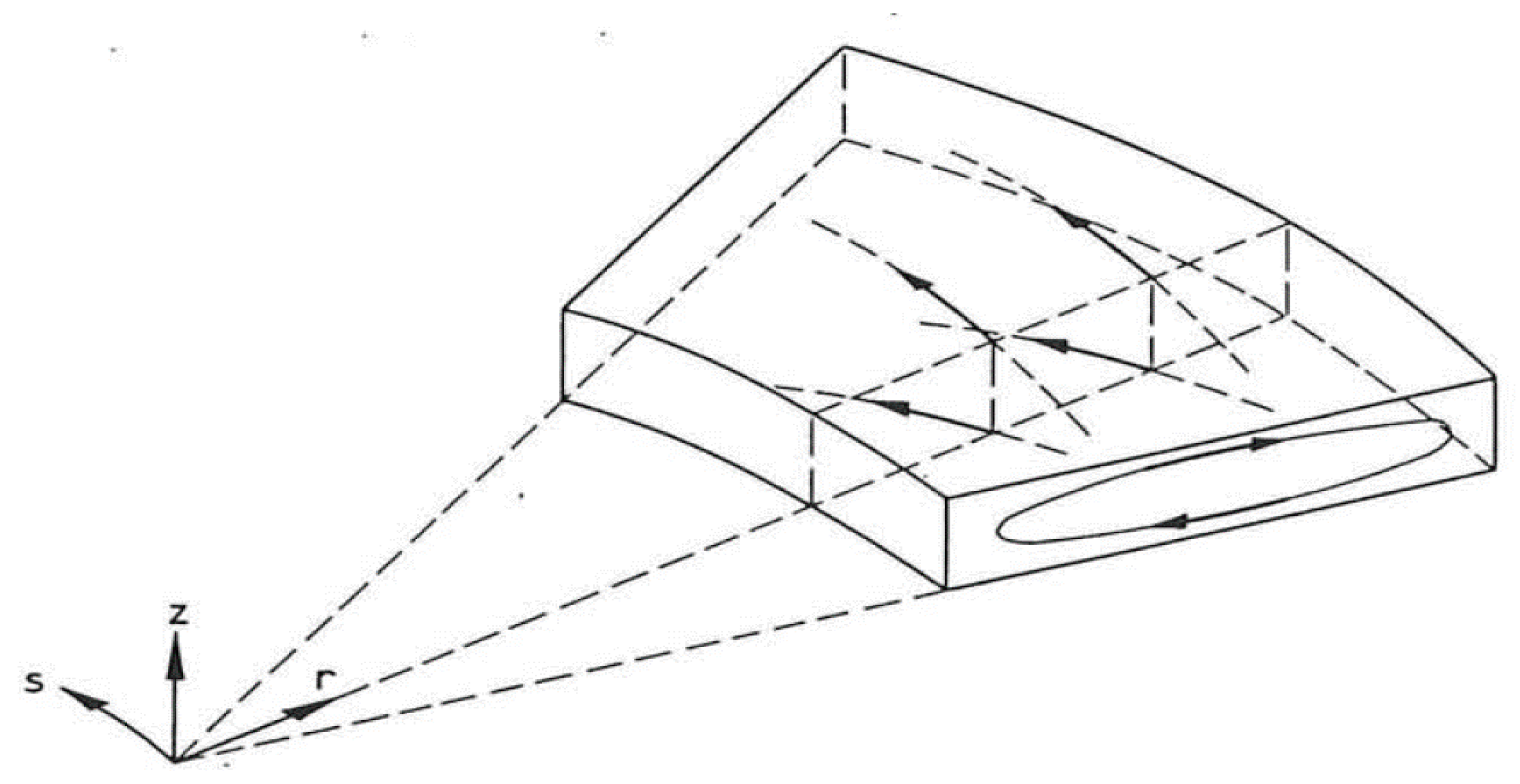
Figure 2.
Centripetal and centrifugal acceleration (Jongbloed, 1996) [28].
Figure 2.
Centripetal and centrifugal acceleration (Jongbloed, 1996) [28].

Figure 3.
Secondary flow cells (based on Blanckaert (2011) [31].
Figure 3.
Secondary flow cells (based on Blanckaert (2011) [31].
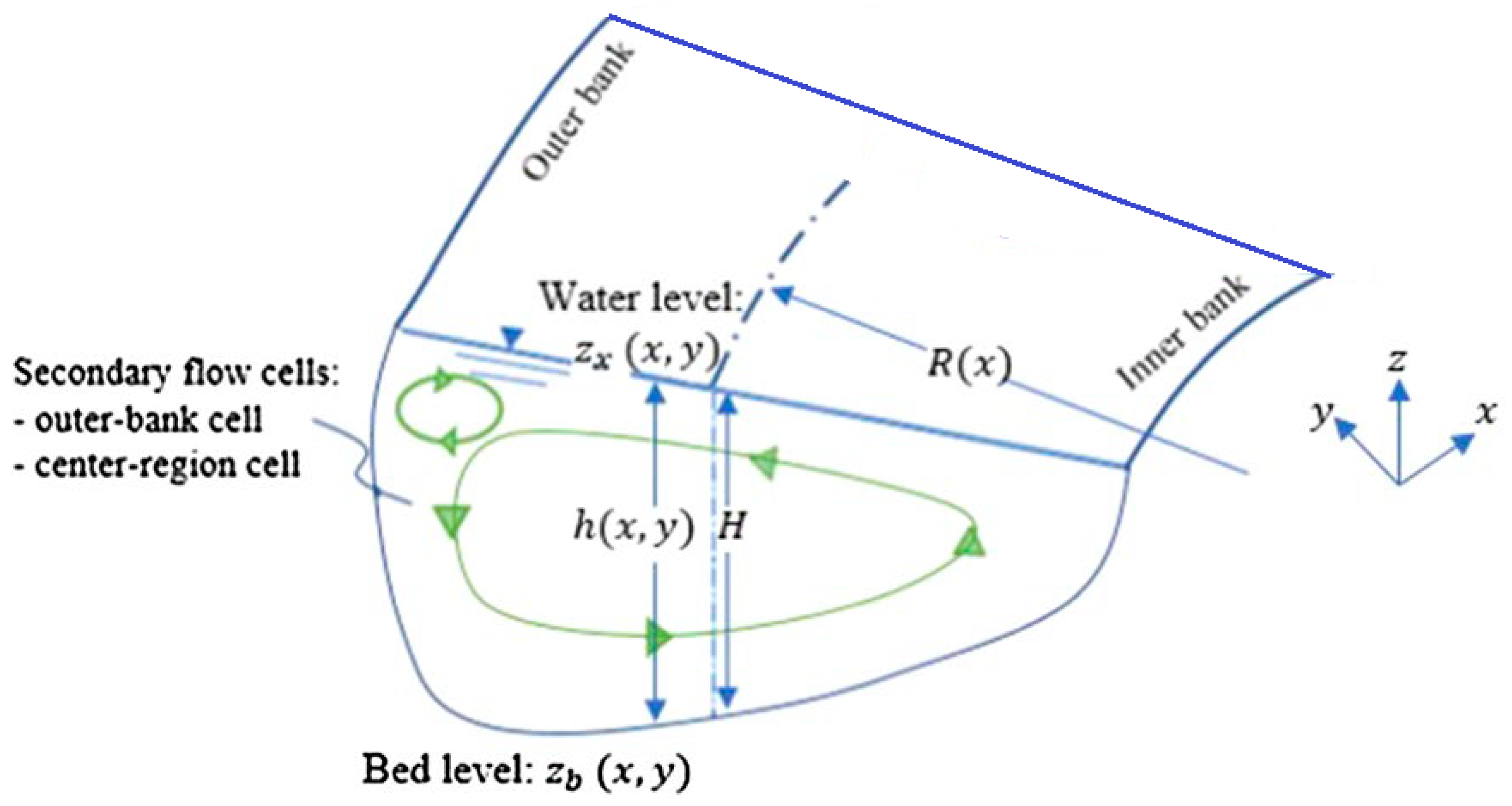
Figure 4.
Main-flow isovels ( ![Water 13 00884 i001]() ) and secondary-flow streamlines (
) and secondary-flow streamlines ( ![Water 13 00884 i002]() ) in the inner wall region of a shallow channel (d/B = 0.1) (De Vriend, 1980) [4].
) in the inner wall region of a shallow channel (d/B = 0.1) (De Vriend, 1980) [4].
 ) and secondary-flow streamlines (
  ) in the inner wall region of a shallow channel (d/B = 0.1) (De Vriend, 1980) [4].
Figure 4.
Main-flow isovels ( ![Water 13 00884 i001]() ) and secondary-flow streamlines (
) and secondary-flow streamlines ( ![Water 13 00884 i002]() ) in the inner wall region of a shallow channel (d/B = 0.1) (De Vriend, 1980) [4].
) in the inner wall region of a shallow channel (d/B = 0.1) (De Vriend, 1980) [4].
) and secondary-flow streamlines ( ) in the inner wall region of a shallow channel (d/B = 0.1) (De Vriend, 1980) [4].
Figure 5.
S-shaped channel used in Ghanmi’s (1999) [57] study from top view and characteristics of sections, which are used to compare calculated and measured data (Reproduced from Khosronejad et al. (2007) [20] with permission from ASCE).
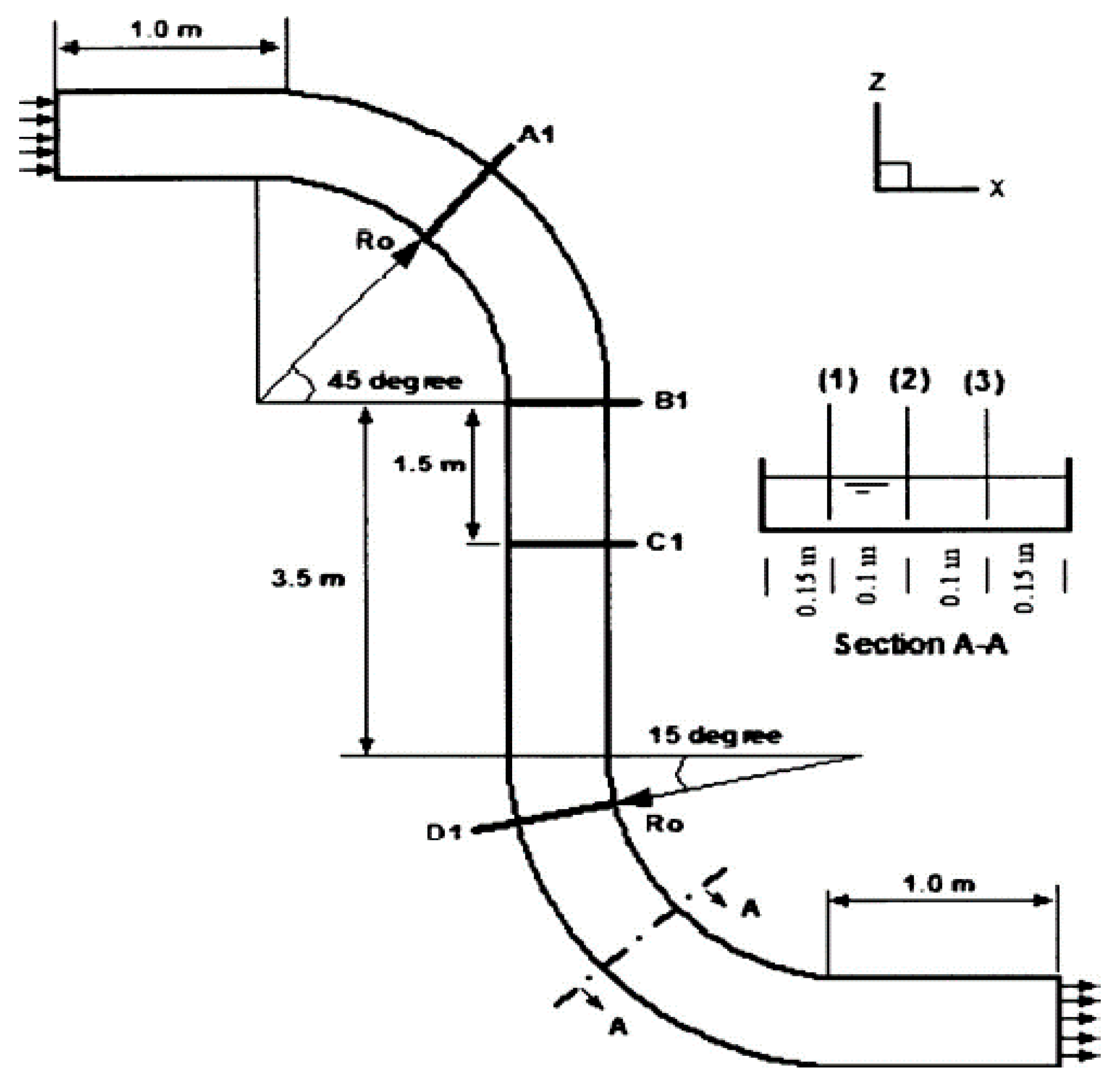
Figure 6.
Surface elevation and velocity vector field (Reproduced from Duan (2004) [50] with permission from ASCE).
Figure 6.
Surface elevation and velocity vector field (Reproduced from Duan (2004) [50] with permission from ASCE).
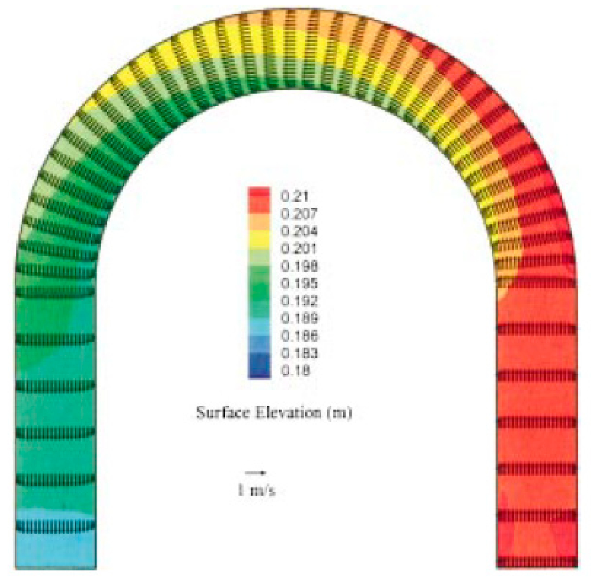
Figure 7.
Surface elevation and velocity distribution (Reproduced from Duan (2004) [50] with permission from ASCE).
Figure 7.
Surface elevation and velocity distribution (Reproduced from Duan (2004) [50] with permission from ASCE).

Figure 8.
Characteristics of geometrical setup (Gholami et al., 2014) [52].
Figure 8.
Characteristics of geometrical setup (Gholami et al., 2014) [52].

Figure 9.
Model setup for the closed curved channel (Shaheed et al., 2018) [55].
Figure 9.
Model setup for the closed curved channel (Shaheed et al., 2018) [55].
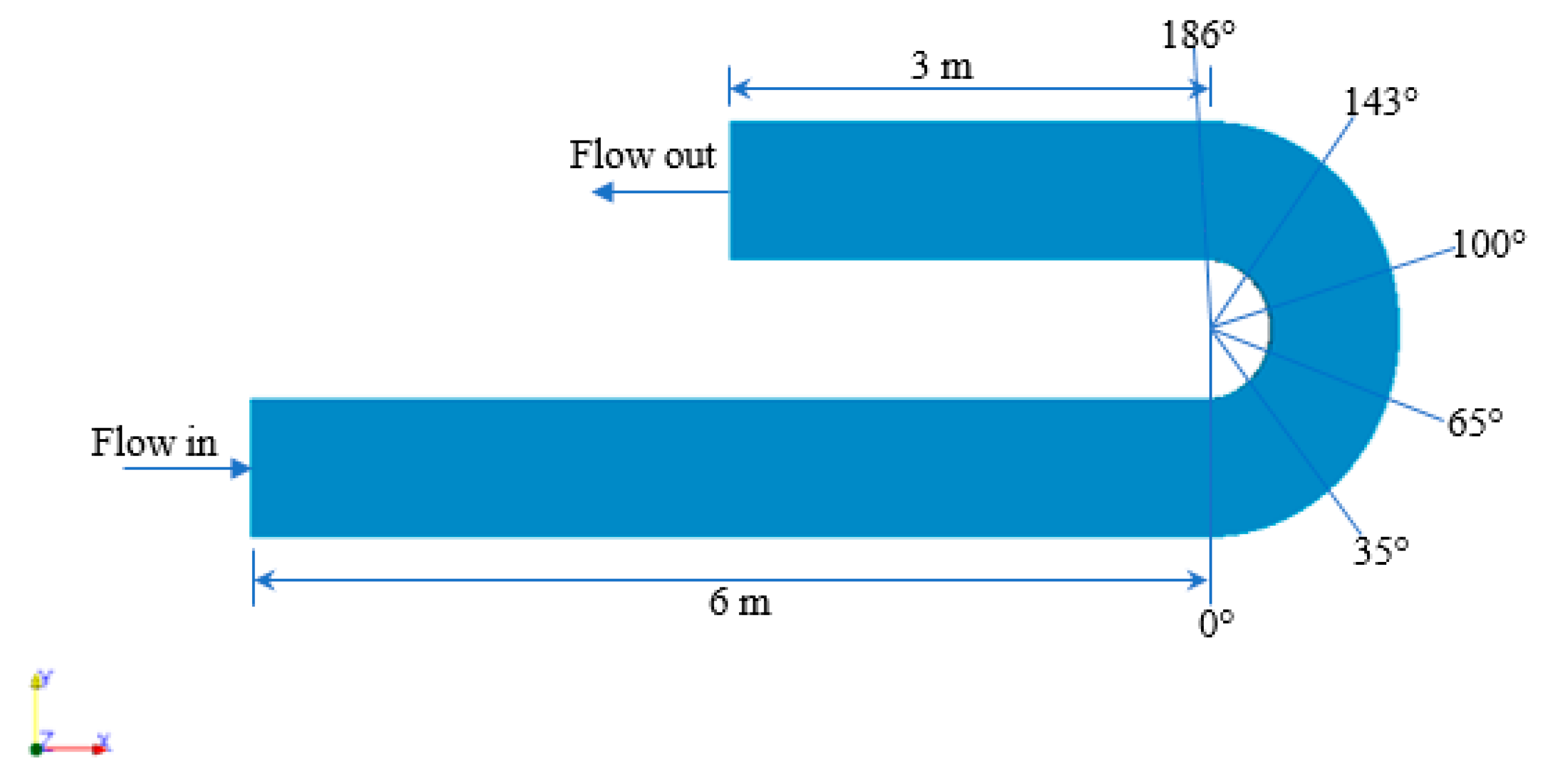
Figure 10.
Velocity distribution for closed curved channel (Shaheed et al., 2018) [55].
Figure 10.
Velocity distribution for closed curved channel (Shaheed et al., 2018) [55].
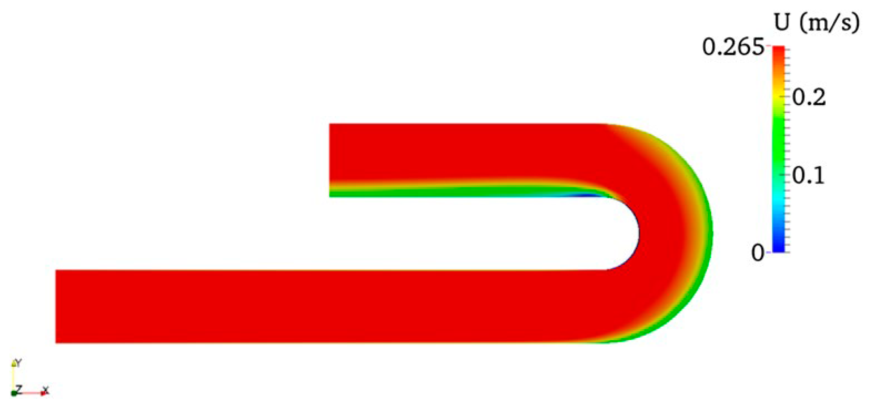
Figure 11.
A comparison of resultant velocities across dimensionless channel width for the Rozovskii channel [2]. (a) at θ = 0°; (b) at θ = 35°; (c) at θ = 65°; (d) at θ = 100°; (e) at θ = 143°; and (f) at θ = 186° (Shaheed et al., 2018) [55].
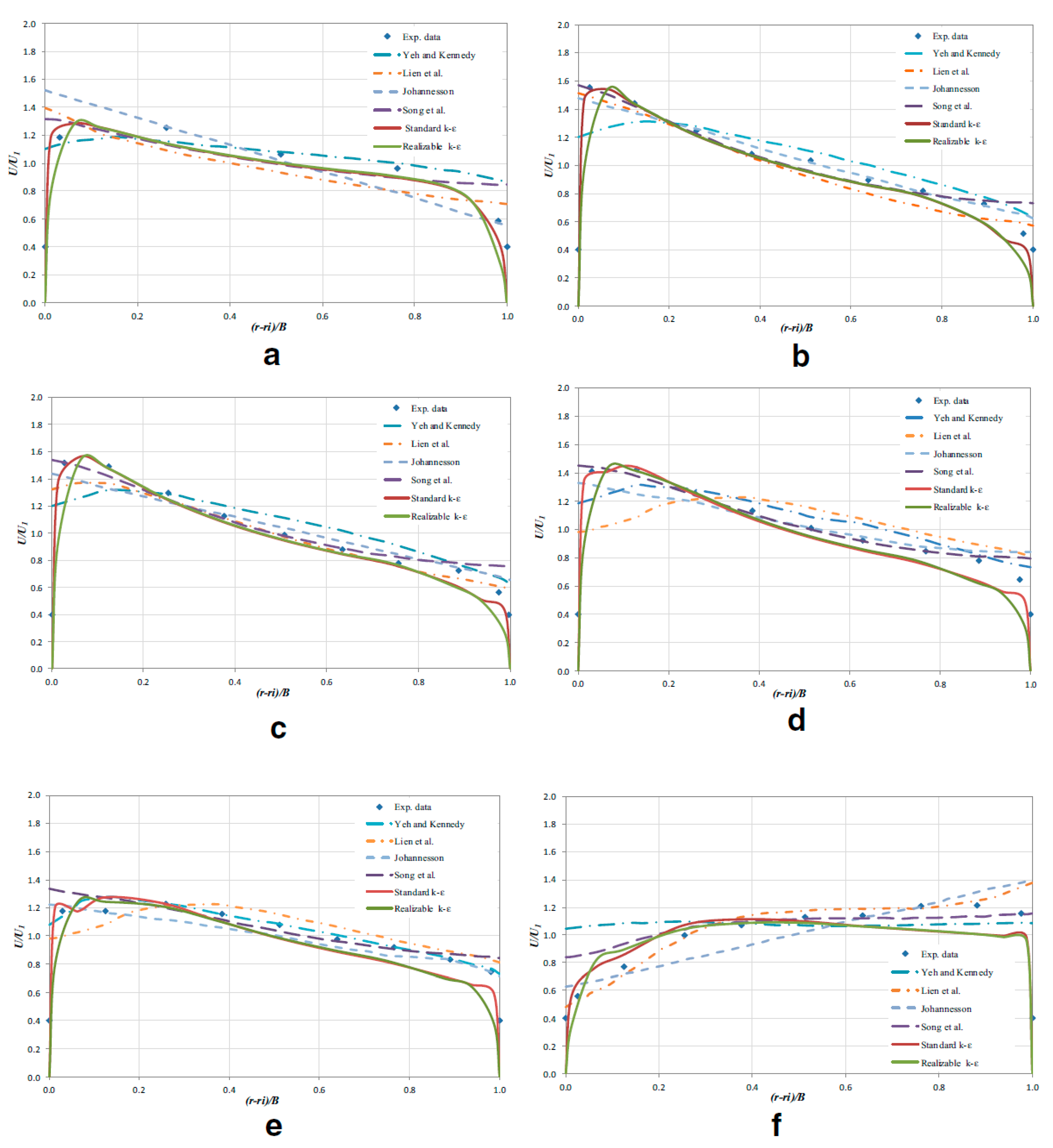
Figure 12.
Flow and concentration field (Reproduced from Duan (2004) [50] with permission from ASCE).
Figure 12.
Flow and concentration field (Reproduced from Duan (2004) [50] with permission from ASCE).

Figure 13.
Comparison of simulated and measured depth-averaged velocity and concentration field (Reproduced from Duan (2004) [50] with permission from ASCE).
Figure 13.
Comparison of simulated and measured depth-averaged velocity and concentration field (Reproduced from Duan (2004) [50] with permission from ASCE).

Figure 14.
Geometric parameters and characteristics of 90° bend channel used in Matsuura 2004 [73] study (Reproduced from Khosronejad et al. (2007) [20] with permission from ASCE).
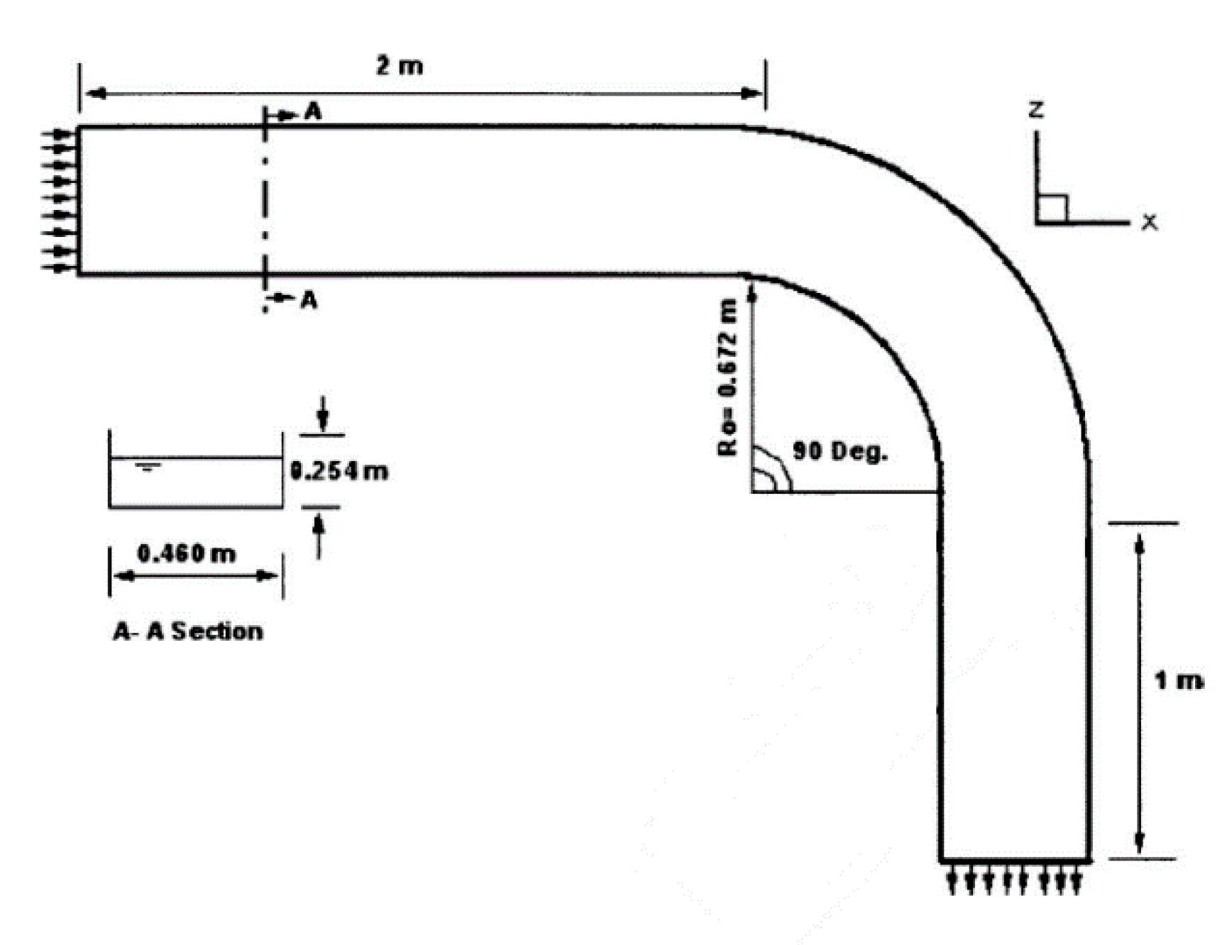
Figure 15.
Geometric parameters and characteristics of 135° bend channel used in Matsuura 2004 [72] study (Reproduced from Khosronejad et al. (2007) [20] with permission from ASCE).
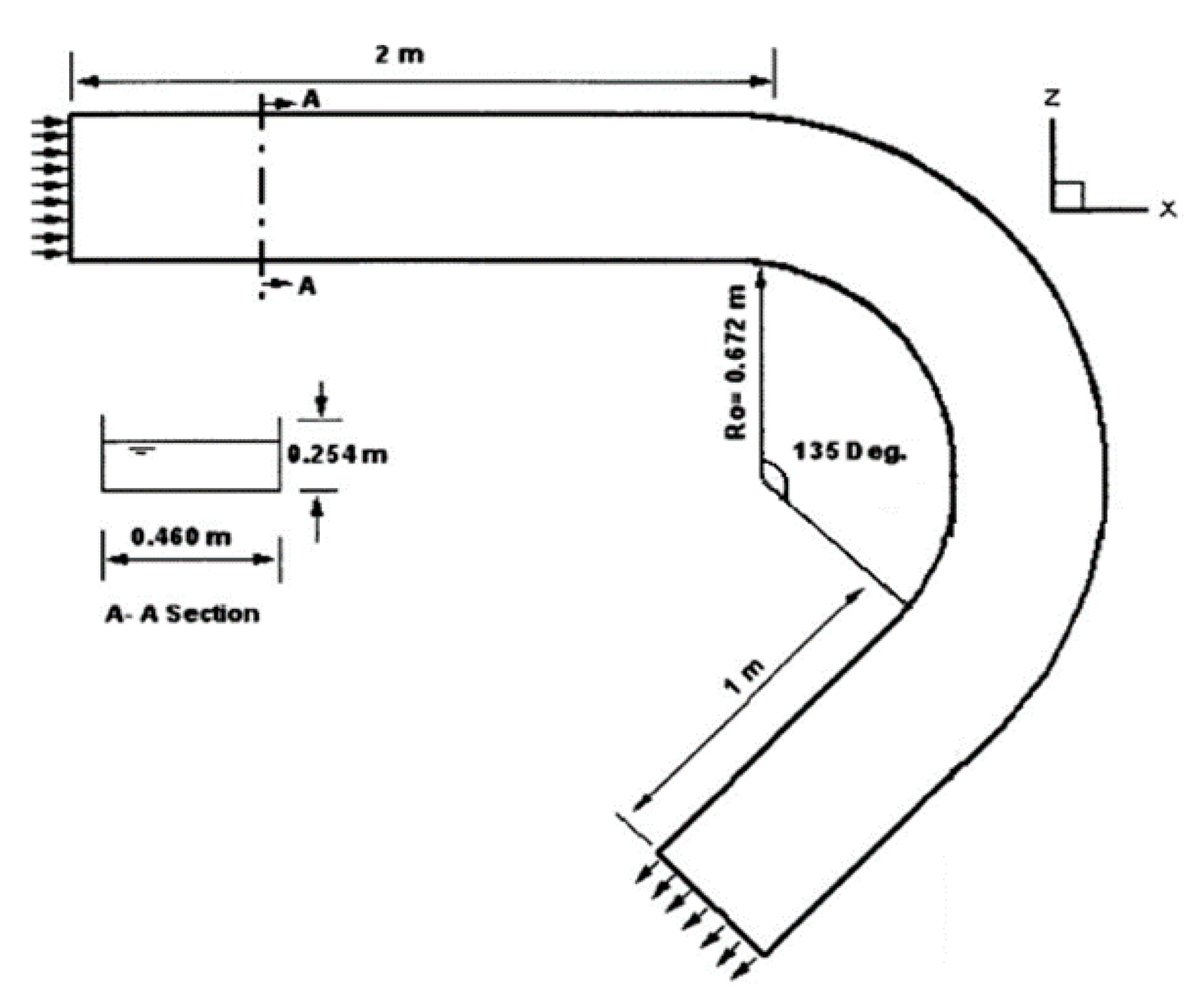
Figure 16.
Bottom topography of the laboratory flume. The arrow denotes the flow direction (Reproduced from van Balen et al. (2010) [77] with the permission of AIP Publishing).
Figure 16.
Bottom topography of the laboratory flume. The arrow denotes the flow direction (Reproduced from van Balen et al. (2010) [77] with the permission of AIP Publishing).


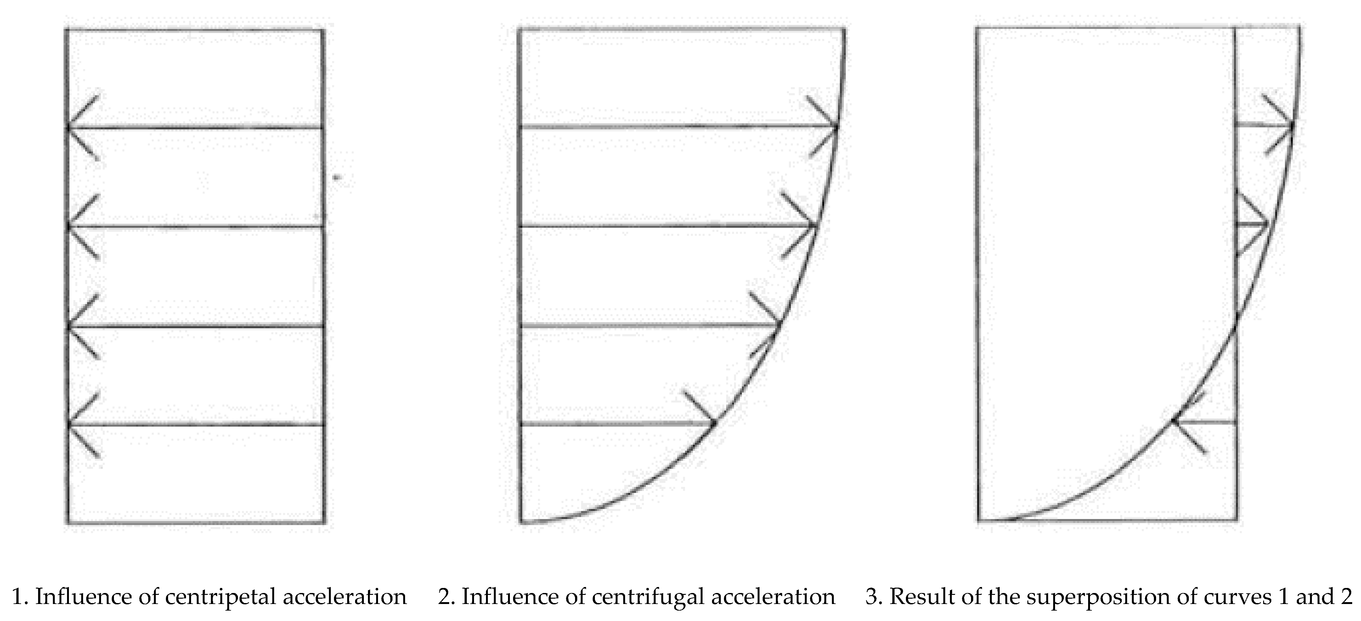
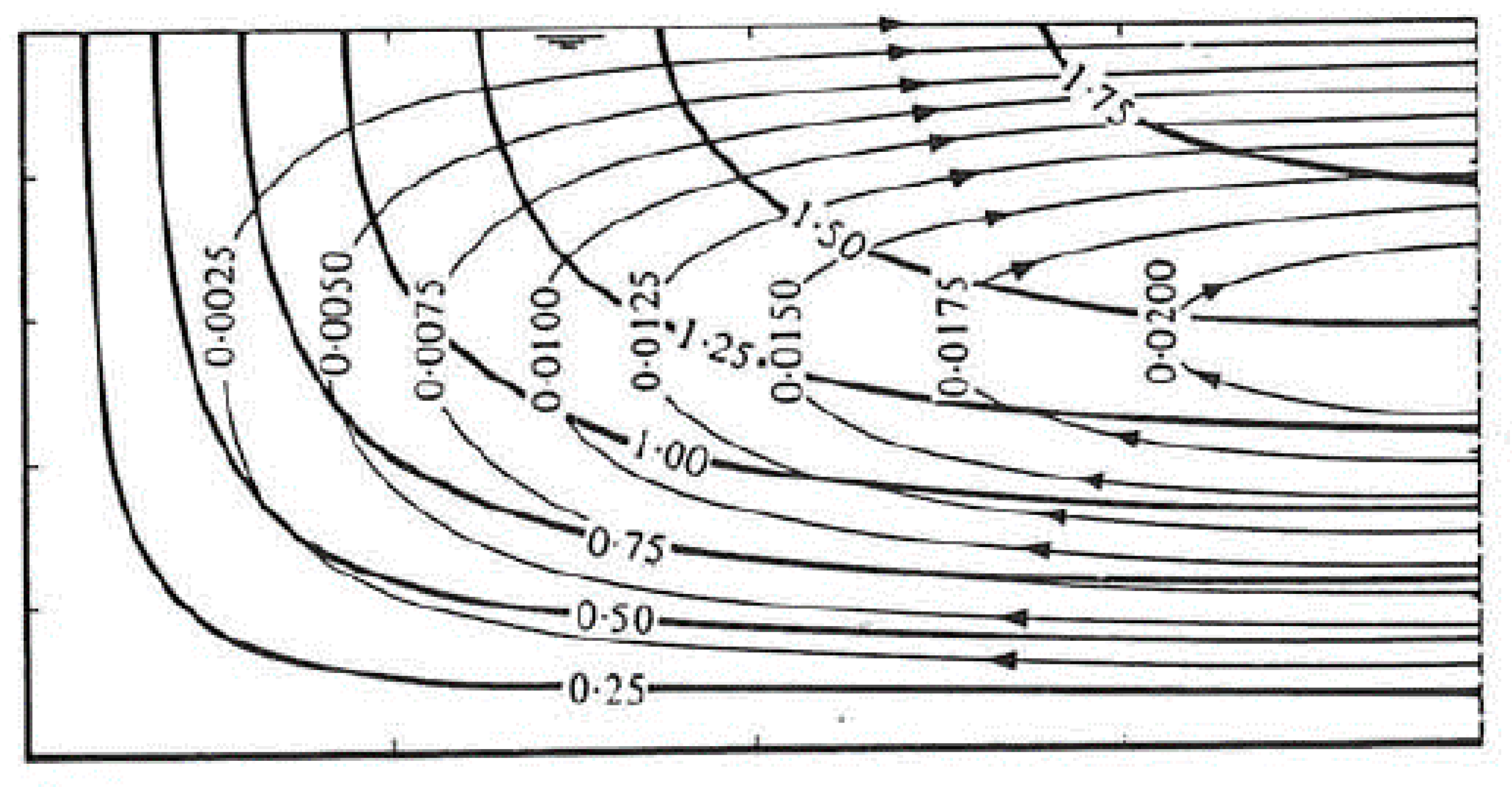
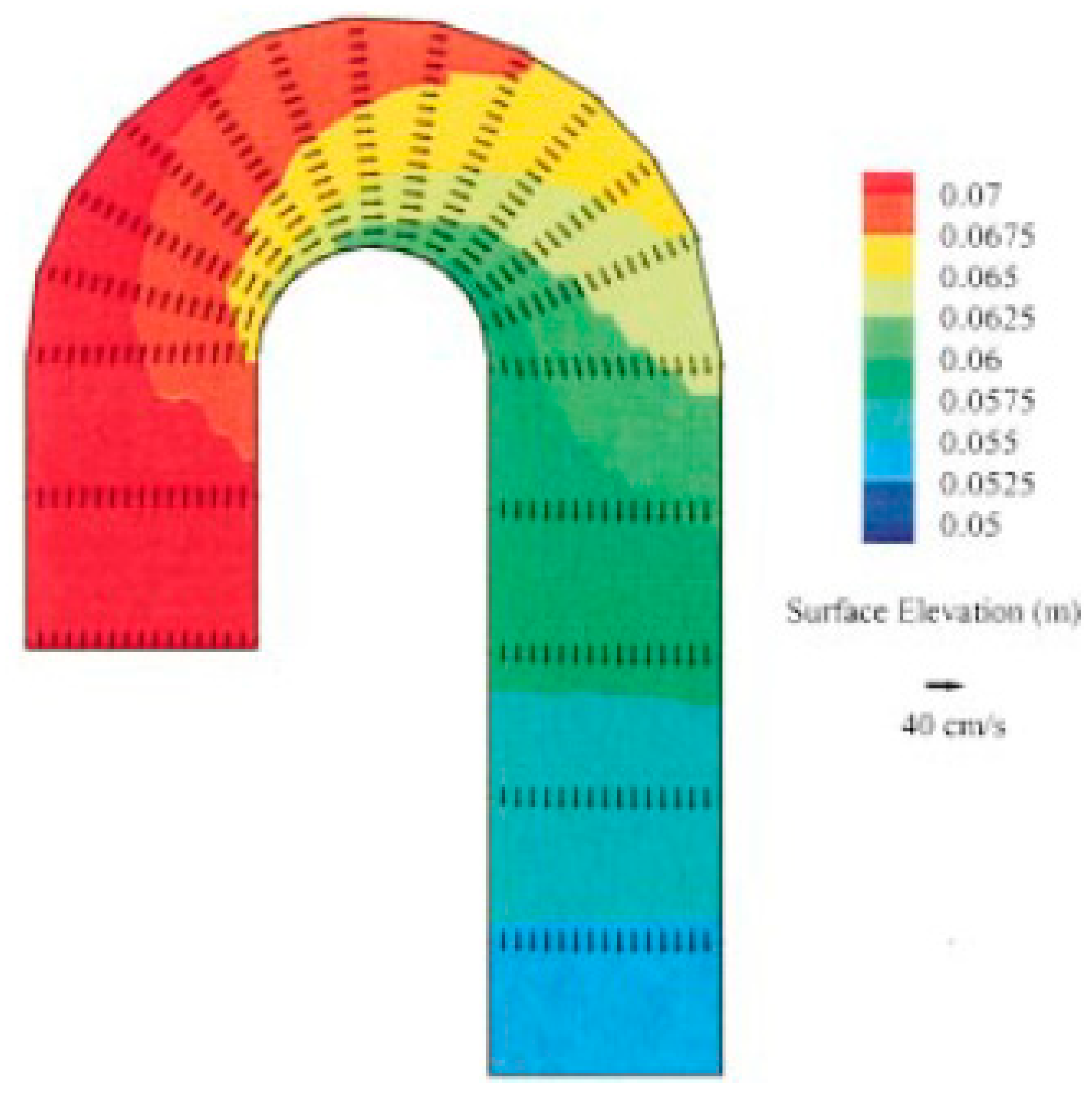
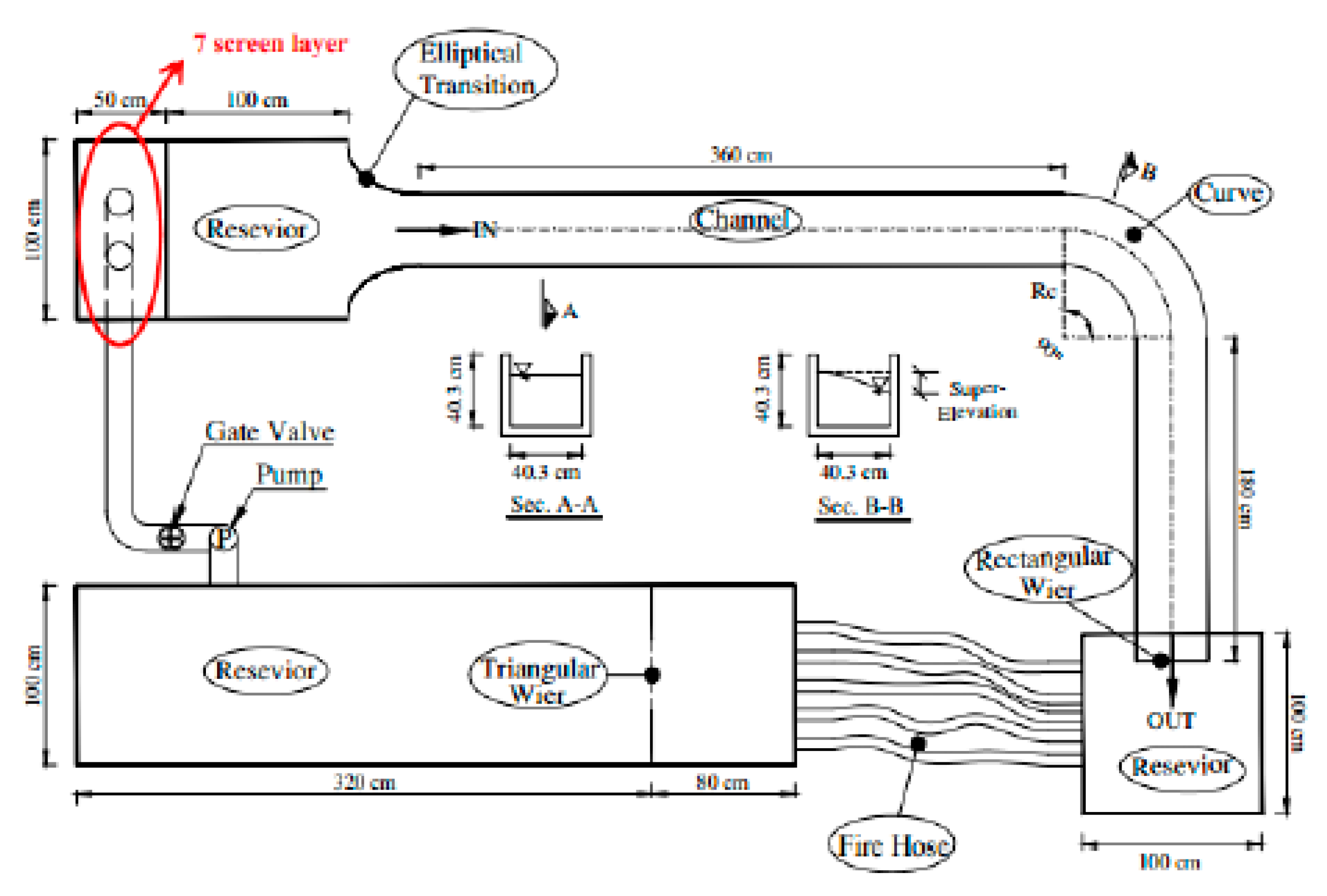
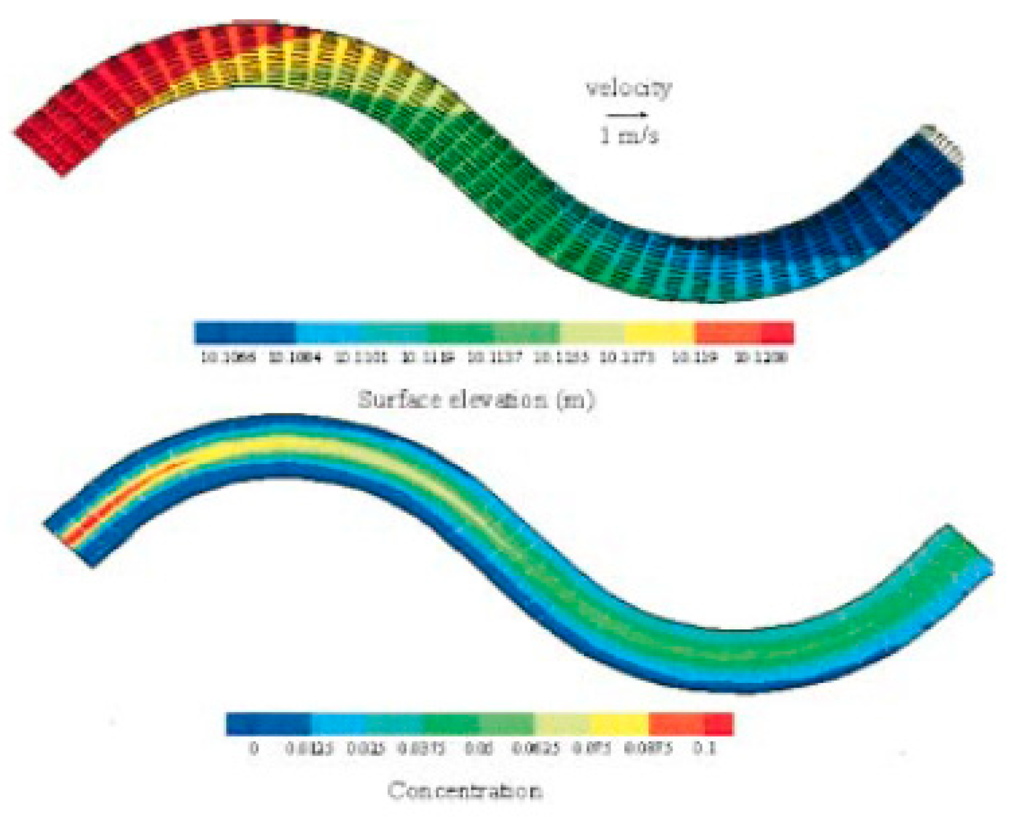
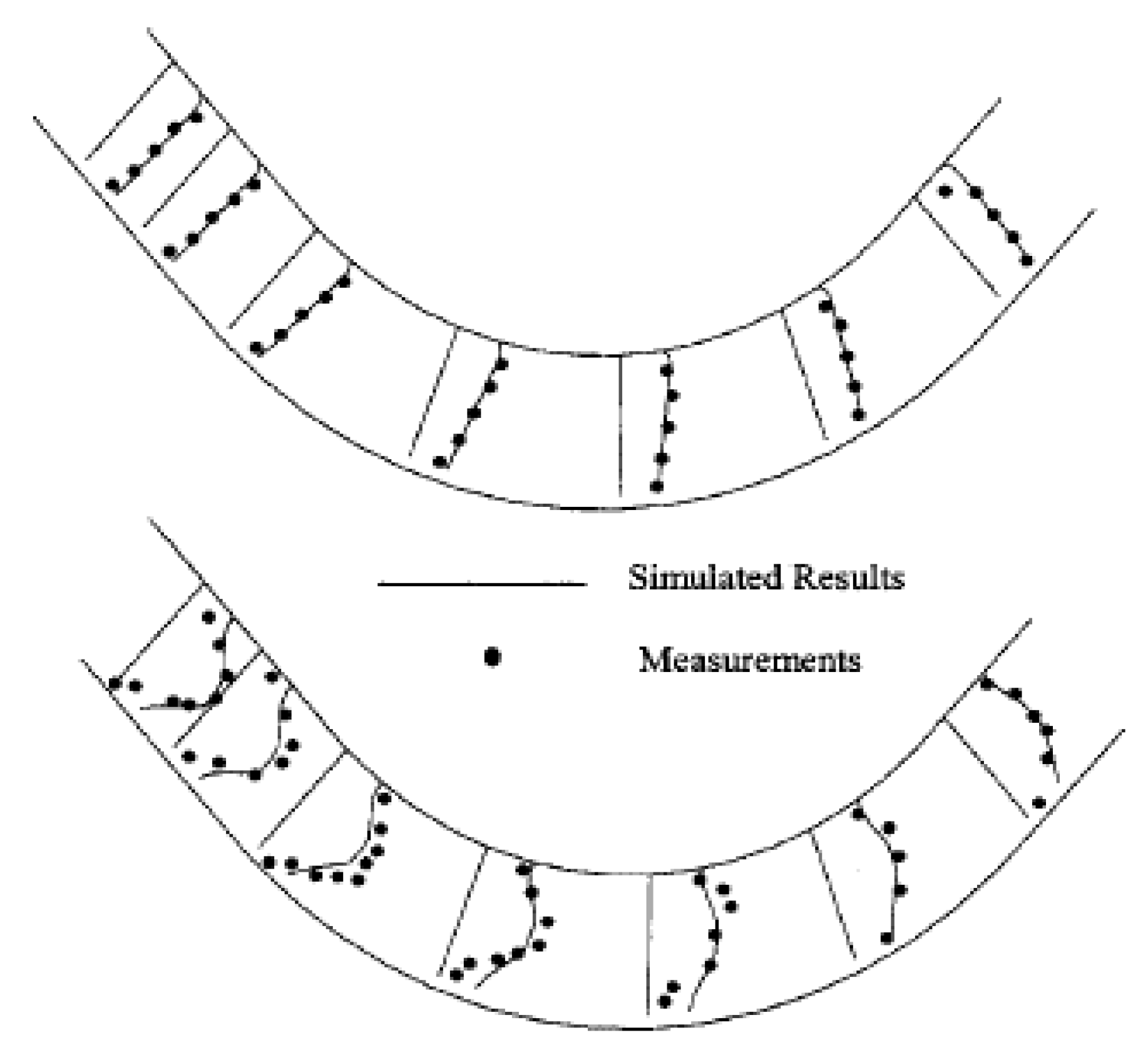
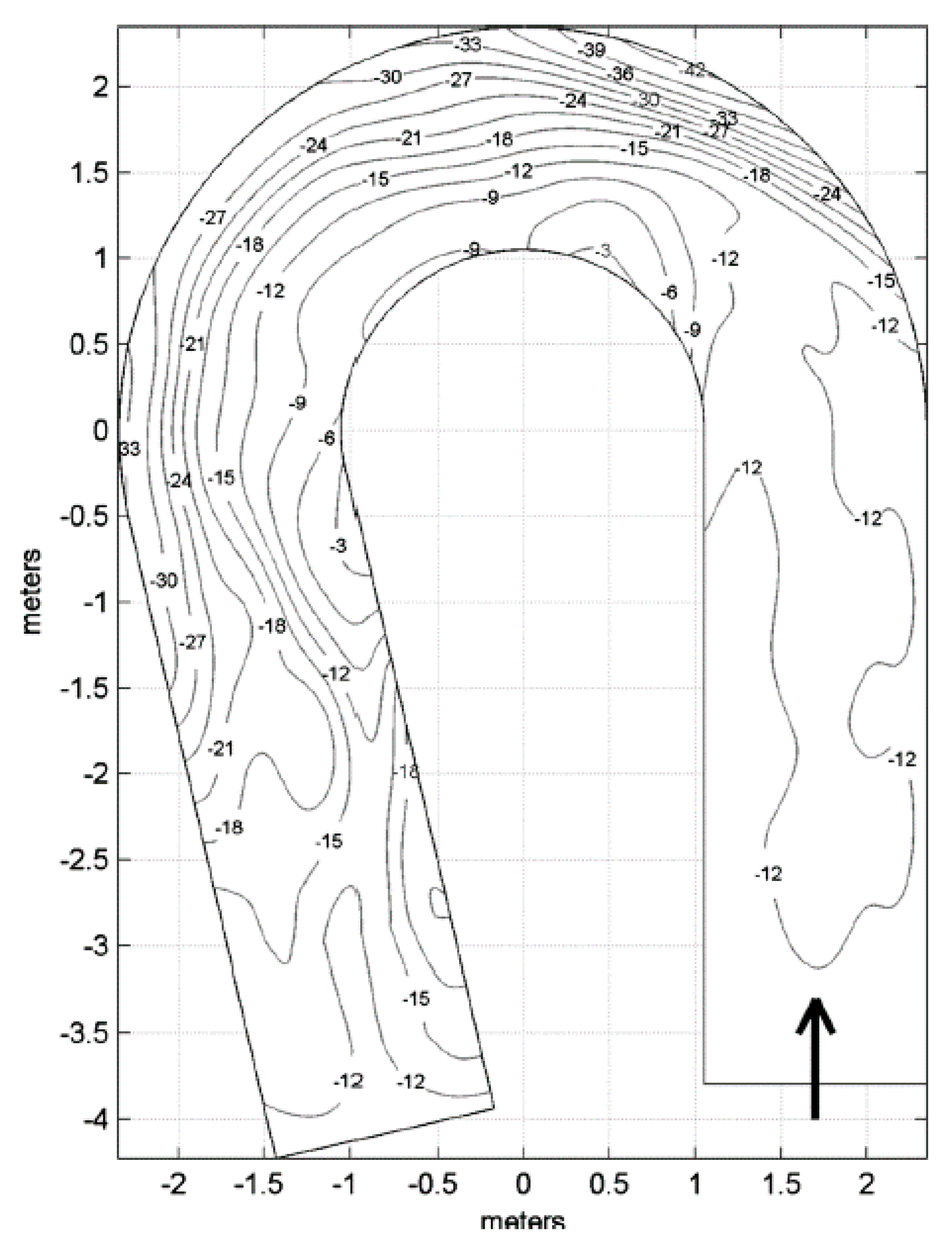
Table 1.
Summary of selected studies about secondary flow in curved channels used in Section 5.1.
Table 1.
Summary of selected studies about secondary flow in curved channels used in Section 5.1.
| Shape of Channel | Numerical Model | Key Findings | Reference |
|---|---|---|---|
| S-shape with two identical 90° reverse bends | Standard k-ε low-Reynolds number k-ω | k-ω model is better than the k-ɛ model in simulating the transverse velocities, which form the secondary flow phenomenon. | (Khosronejad et al., 2007) [20] |
| U-shaped mildly curved channel having a U-shape | Depth-averaged 2D numerical model | Generally, there was an agreement between the simulated and measured surface elevations at the inner, outer bank, and centerline. | (Duan, 2004) [50] |
| U-shaped sharply curved channel in 180° bend | Depth-averaged 2D numerical model | There is good agreement between the simulated and measured results. | (Duan, 2004) [50] |
| A channel in 90° bend | low-Reynolds number k-ω, k-ε (realizable), k-ε (RNG) and LES models | The performance of k-ε (RNG), k-ω and k-ε (realizable) models was good in simulating the flow in the bend, while the LES model has not shown its capability in simulating the flow in channel bends, especially after the curve. | (Ghaneeizad et al., 2010) [51] |
| A channel in 90° bend | k-ε (RNG) | The results of the comparison between the numerical model and the experimental data indicated that there is an acceptable level of agreement. | (Gholami et al., 2014) [52] |
| The flume of two successive 180° bends | RANS including (standard k-ε, standard k-ω), LES | Both RANS simulation and LES model performed well in predicting the primary and an outer bank secondary cell at the peak of the bend. | (Stoesser et al., 2010) [53] |
| The flume of two successive 180° bends | Standard k-ε model, and the non-linear k-ε model | The two models showed the counter-clockwise secondary cell inherited from the first bend, while only the non-linear k-ε model showed the counter-rotating secondary cell of the previous bend, which is coincident with the higher primary velocities. | (Fraga et al., 2012) [54] |
| U-shaped sharply curved channel in 180° bend | Standard k–ε model and the realizable k–ε model | The standard k–ε model performed better than the realizable k-ε model. | (Shaheed et al., 2018) [55] |
| A channel in 135° bend with side slopes | Standard k-ε, (RNG) k-ε, realizable k-ε, k-ω, and (SST) k-ω) | The realizable k-ε model was the best in capturing the outer bank cells among the tested models. | (Yan et al., 2020) [56] |
| A mild 180° bend with a rectangular section and rotating annular flumes | LES and RANS (k-ɛ model) | The outer bank cell was reproduced well by the LES computations, unlike the RANS computations. | (Booij, 2003) [7] |
Table 2.
Summary of studies about pollutant dispersion in curved channels used in Section 5.2.
Table 2.
Summary of studies about pollutant dispersion in curved channels used in Section 5.2.
| Shape of Channel | Numerical Model | Key Findings | Reference |
|---|---|---|---|
| The flume consists of a single meander of two 90° bends in alternating directions | Depth-averaged 2D numerical model | There is an agreement between the simulated and measured results. | (Duan, 2004) [50] |
| Three different meander situations were used including wide, shallow channels with a smooth bed, and two narrow channels with one having a smooth and the other a rough bed. | Standard k-ɛ turbulence model | The agreement was fairly good in the case of the smooth bed for the vertical profiles of longitudinal velocity, but it was not so good for the case of the rough bed. | (Demuren and Rodi, 1986) [71] |
Table 3.
Summary of studies about sediment transport in curved channels used in Section 5.3.
Table 3.
Summary of studies about sediment transport in curved channels used in Section 5.3.
| Shape of Channel | Numerical Model | Key Findings | Reference |
|---|---|---|---|
| A channel in 90° bend | Standard k-ε model and the low-Reynolds number k-ω model | The low-Reynolds k-ω turbulence model is better than the standard k-ε model | (Khosronejad et al., 2007) [20] |
| A channel in 135° bend | Standard k-ε model and the low-Reynolds number k-ω model | The low-Reynolds k-ω turbulence model is better than the standard k-ε model | (Khosronejad et al., 2007) [20] |
| A channel in 180° bend | k-ε turbulence model | There is good agreement between the measurements and the predicted results | (Wu et al., 2000) [40] |
Table 4.
Summary of studies about bend over topography used in Section 5.4.
Table 4.
Summary of studies about bend over topography used in Section 5.4.
| Shape of Channel | Numerical Model | Key Findings | Reference |
|---|---|---|---|
| A channel in 193° bend | The k-ω Shear Stress Transport (SST) model, or the Spalart–Allmaras (SA) model in low-Reynolds number versions | It could be considered that the accuracy and predictive capacity of the model is satisfactory. | (Zeng et al., 2008) [24] |
| A channel in 193° bend | LES model | There is a good qualitative agreement between the LES model and the experimental findings | (van Balen et al., 2010) [77] |
Table 5.
Hydraulic parameters of the three simulation runs. Q is the discharge, Vav the bulk velocity, H the mean water depth, B the width of the channel, Ks the roughness height of the bed, and Re the Reynolds number based on the bulk velocity and the mean water depth (van Balen et al., 2010) [77].
| Run | Q (l/s) | Vav (m/s) | H (m) | B (m) | Ks (m) | Re |
|---|---|---|---|---|---|---|
| A | 89 | 0.49 | 0.141 | 1.3 | 0.037 | 68,000 |
| B | 89 | 0.49 | 0.141 | 1.3 | 0.006–0.037 | 68,000 |
| C | 89 | 0.49 | 0.141 | 1.3 | 0.006 | 68,000 |
Publisher’s Note: MDPI stays neutral with regard to jurisdictional claims in published maps and institutional affiliations. |
© 2021 by the authors. Licensee MDPI, Basel, Switzerland. This article is an open access article distributed under the terms and conditions of the Creative Commons Attribution (CC BY) license (http://creativecommons.org/licenses/by/4.0/).
Share and Cite
MDPI and ACS Style
Shaheed, R.; Mohammadian, A.; Yan, X. A Review of Numerical Simulations of Secondary Flows in River Bends. Water 2021, 13, 884. https://doi.org/10.3390/w13070884
AMA Style
Shaheed R, Mohammadian A, Yan X. A Review of Numerical Simulations of Secondary Flows in River Bends. Water. 2021; 13(7):884. https://doi.org/10.3390/w13070884
Chicago/Turabian StyleShaheed, Rawaa, Abdolmajid Mohammadian, and Xiaohui Yan. 2021. "A Review of Numerical Simulations of Secondary Flows in River Bends" Water 13, no. 7: 884. https://doi.org/10.3390/w13070884
Note that from the first issue of 2016, this journal uses article numbers instead of page numbers. See further details here.