
Modelling the Impacts of Climate Change on Shallow Groundwater Conditions in Hungary

1
Department of Engineering Geology and Geotechnics, Budapest University of Technology and Economics, Műegyetem rkp. 1, 1111 Budapest, Hungary
2
Jakab és Társai Kft., 32 Jászóvár utca, 2100 Gödöllő, Hungary
*
Author to whom correspondence should be addressed.
Water 2021, 13(5), 668; https://doi.org/10.3390/w13050668
Submission received: 15 December 2020
/
Revised: 25 January 2021
/
Accepted: 5 February 2021
/
Published: 1 March 2021
(This article belongs to the Special Issue Climate Change Impacts on Water Resources)
Abstract
:The purpose of the present study was to develop a methodology for the evaluation of direct climate impacts on shallow groundwater resources and its country-scale application in Hungary. A modular methodology was applied. It comprised the definition of climate zones and recharge zones, recharge calculation by hydrological models, and the numerical modelling of the groundwater table. Projections of regional climate models for three different time intervals were applied for the simulation of predictive scenarios. The investigated regional climate model projections predict rising annual average temperature and generally dropping annual rainfall rates throughout the following decades. Based on predictive modelling, recharge rates and groundwater levels are expected to drop in elevated geographic areas such as the Alpokalja, the Eastern parts of the Transdanubian Mountains, the Mecsek, and Northern Mountain Ranges. Less significant groundwater level drops are predicted in foothill areas, and across the Western part of the Tiszántúl, the Duna-Tisza Interfluve, and the Szigetköz areas. Slightly increasing recharge and groundwater levels are predicted in the Transdanubian Hills and the Western part of the Transdanubian Mountains. Simulation results represent groundwater conditions at the country scale. However, the applied methodology is suitable for simulating climate change impacts at various scales.
1. Introduction
Groundwater is the world’s largest distributed store of fresh water, and as such, it plays a central part in sustaining ecosystems and human population. Groundwater comprises almost one-third of the Planet’s freshwater reserves, and 96% of liquid-phase freshwater [1].
The climate projections of the Intergovernmental Panel on Climate Change (IPCC) indicate a significant temperature rise and alterations in the amount and frequency of precipitation throughout the rest of the 21st century [2,3,4]. Changing climate variables influence the hydrological cycle through impacting on [5]:
- Surface runoff;
- Evapotranspiration;
- Groundwater recharge;
- Soil water content;
- Surface water levels and quality;
- Groundwater levels and quality;
- Snow and ice cover.
Precipitation has a direct impact on groundwater recharge and an indirect impact on human groundwater withdrawals. Recharge is very sensitive to precipitation, and small changes in rainfall can result in more significant changes as far as recharge is concerned [6]. Higher temperature increases evapotranspiration rates, which may in turn decrease recharge rates [7]. Air temperature may significantly modify the hydrologic cycle in areas dominated by snow fall and melting [8,9,10,11,12].
There is solid scientific evidence that the global average temperature of the Earth’s surface has increased by about 0.8 °C since 1900. This also included the warming of the ocean, the decline of Arctic sea ice, a rise in sea level, and several other climate effects. Significant warming took place during the past decades. Scientific investigations proved that the global warming is mainly caused by anthropogenic greenhouse gas emissions [4]. Continued greenhouse gas emissions are predicted to cause further increases in global average surface temperature and significant impact on the regional climate.
2. Goals
The present paper discusses the methodology utilized for the simulation of groundwater table from measured climate data series and regional climate model outputs. The developed methodology was applied to calculate the water table at the country scale under various climate conditions. The entire geographic area of Hungary was applied as a test site in order to demonstrate the application of the developed methodology. The aim of water table modelling was to evaluate climate change impacts on shallow groundwater conditions. The methodology presented in this study is applicable at various scales and climate scenarios, and can be applied for the investigation of climate impacts on shallow groundwater resources.
3. Test Site
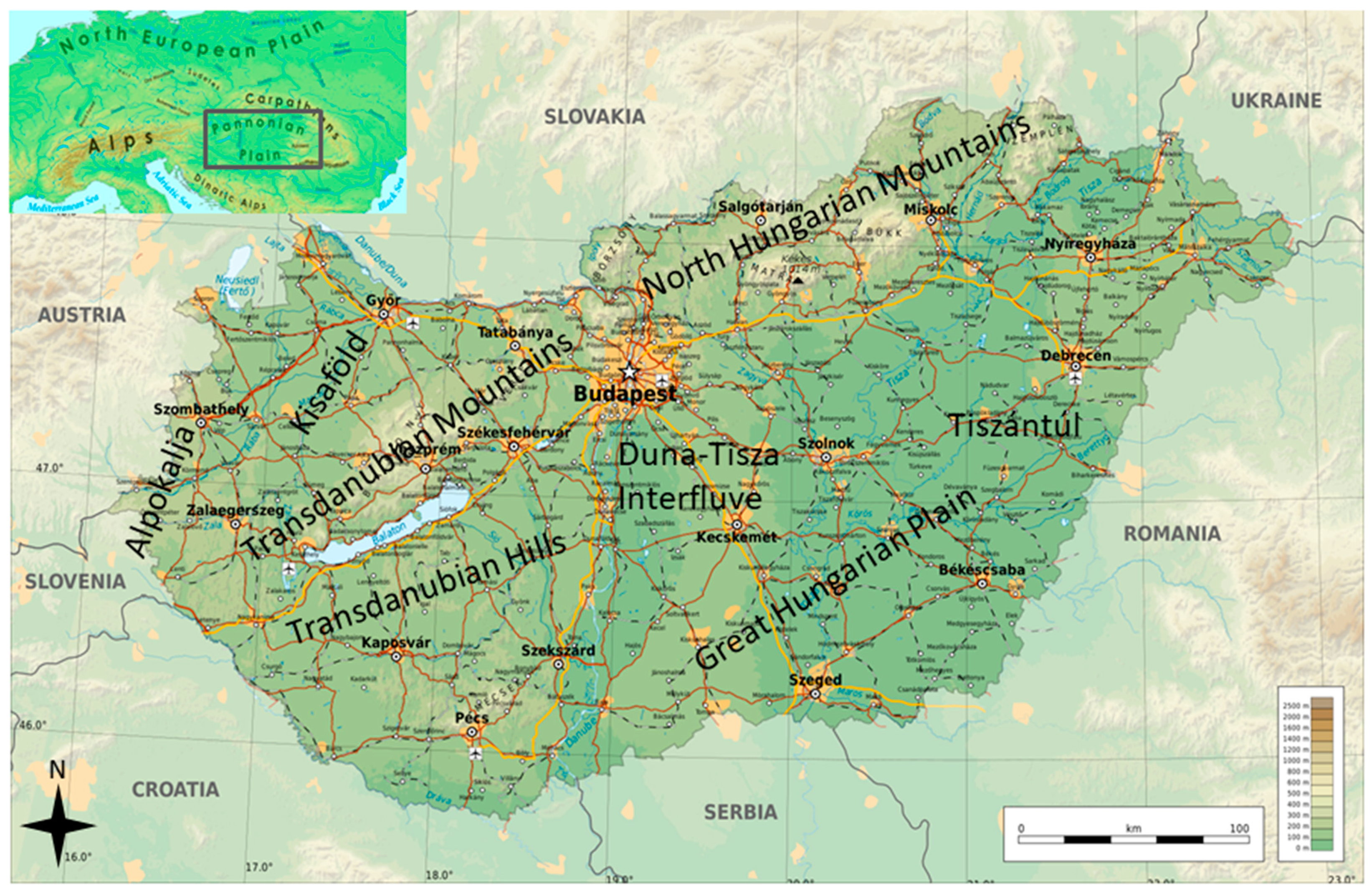
Hungary is a country located in Central Europe with a land area of 93,030 km2. It measures about 250 km in the north–south and 524 km in the east–west direction. It shares borders with Austria to the west, Serbia, Croatia and Slovenia to the south and southwest, Romania to the southeast, Ukraine to the northeast, and Slovakia to the north. The Transdanubian region lies in the western part of the country. The Great Hungarian Plain contains the basin of the Tisza River and its tributaries. It occupies more than half of the country’s territory. Hungarian mountain ranges include the Alpokalja, Transdanubian Mountains, Mecsek and North Hungarian Mountains. Alpokalja is located along the Austrian border. The Transdanubian Mountains stretch from the western ending of Lake Balaton to the Danube river. The North Hungarian Mountains extend along the Slovakian border. The main geographic regions of Hungary are located in Figure 1.
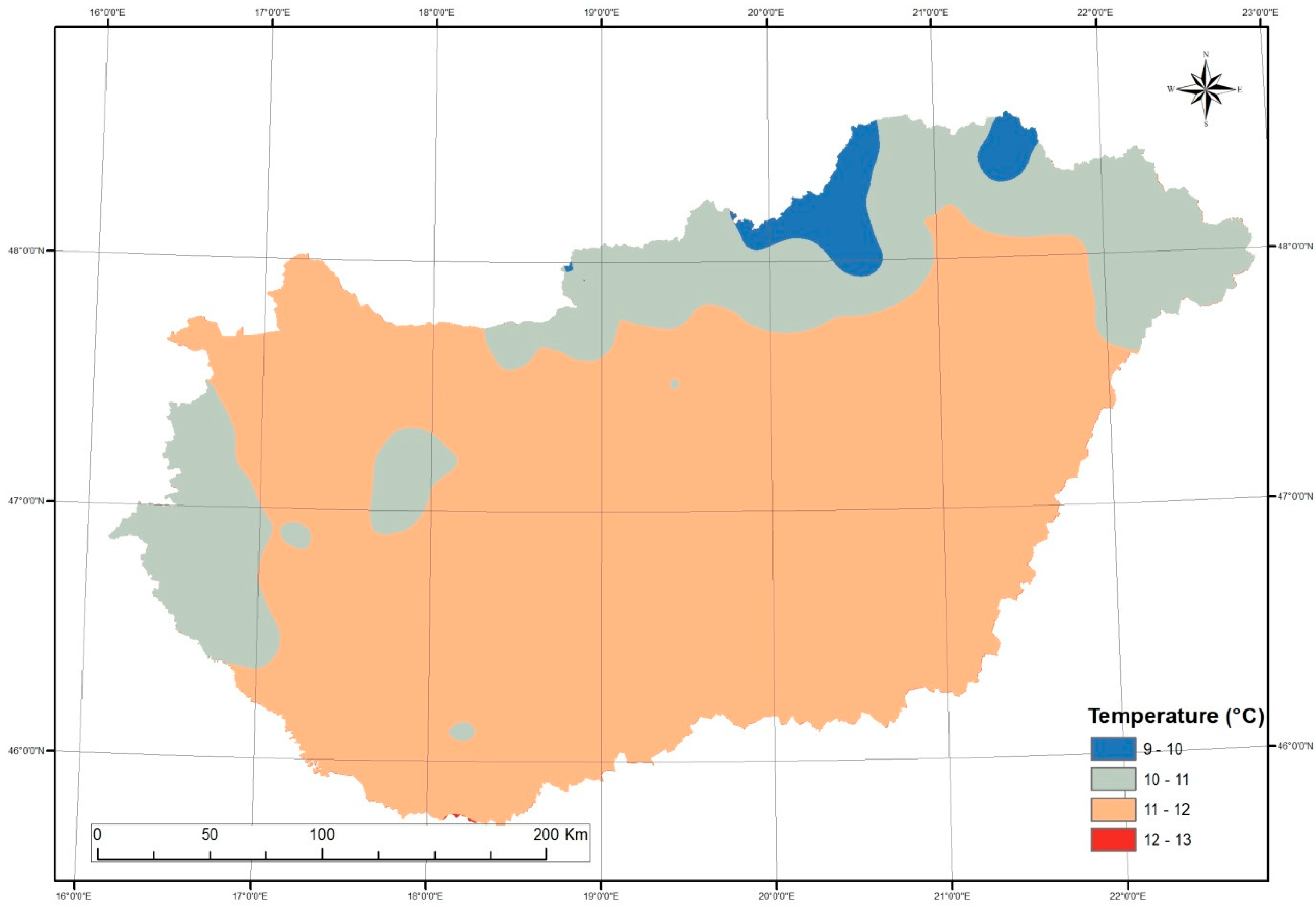
Hungary has a continental climate, with hot summer seasons. The winters are cold and snowy. The average value of annual temperature is 9.7 °C. The extreme values of temperature range between −29 and 42 °C. The average temperature in the summer is 27–35 °C and in the winter it is 0 to −15 °C. The average value of annual rainfall is approximately 600 mm. The annual temperature distribution of Hungary averaged between 1961 and 1990 is indicated in Figure 2.
In central Europe, both the maximum and minimum temperatures warmed over the 20th century. The most significant rise was manifested at minimum temperature. There was more significant summer warming in the first half of the century than in the second half [13].
The analysis of climate data indicates that heat waves became more frequent, longer, and more intense in every season in the entire Carpathian Region. Cold waves show the opposite trend: they are less frequent, shorter, and less intense. The Mediterrania and the Carpathian Region were especially exposed to increasing frequency, duration, and severity of droughts throughout the past decades and particularly after 1990 [14].
The distribution of annual rainfall of Hungary averaged between 1961 and 1990 is indicated in Figure 3. According to observed data, there was a significant decrease in the amount of annual precipitation during the 20th century. The most significant drop in precipitation occurred during the spring seasons, when precipitation dropped by 25% since the beginning of the 20th century. The summer precipitation remained stagnant during the past 100 years. The autumn and winter precipitations showed a decrease by approximately 12–14%. In parallel with decreasing trends, the precipitation events show a more intensive pattern, which is likely to increase run-off rates and the risk of floods. Furthermore, it decreases recharge rates and groundwater resources.
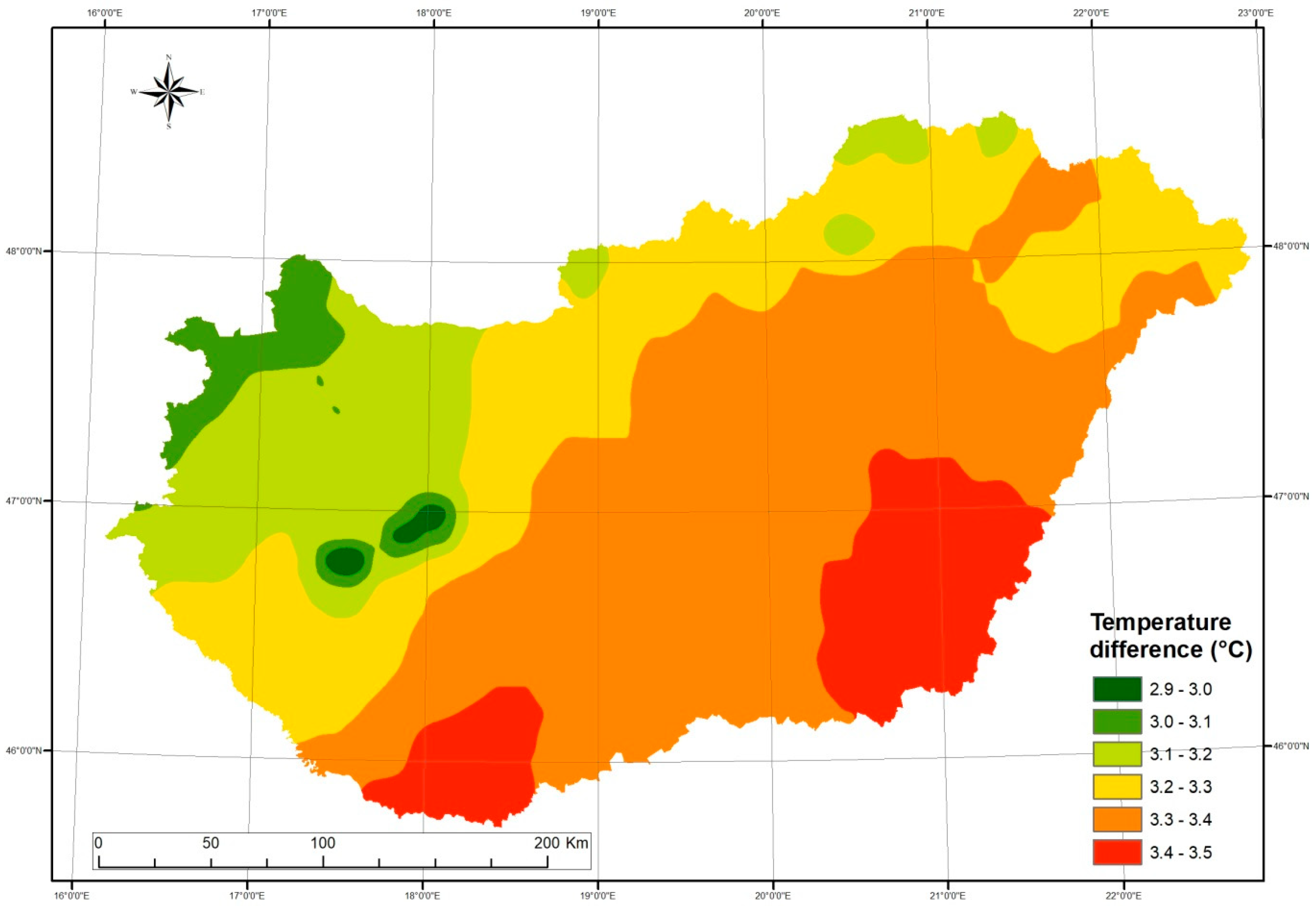
The results of the ALADIN and RegCM regional climate modelling studies [15] indicate that annual average temperature in Hungary is expected to rise by 3–5 °C by the end of the century. Highest warming rates are expected in the summer season. The warming will be more intense in Eastern Hungary than in the western part of the country. The predicted annual temperature change between the reference 1961–1990 and 2071–2100 periods is indicated in Figure 4.
The above climate projections indicate the decrease of annual rainfall amount until the end of the century. At the same time, the temporal distribution of rainfall is predicted to become more balanced with the wettest summer season, which become dryer, while fall seasons become wetter during the following decades. The predicted annual rainfall change between the reference periods of 1961–1990 and 2071–2100 is indicated in Figure 5.
4. Materials and Methods
4.1. Applied Methodology
We developed a modular approach to the quantitative investigation of the influence of climate conditions on the groundwater table:
- Climate zones were determined based on measured and simulated climate variables.
- Recharge zones were delineated based on slope, landuse, and surface geology.
- Recharge was calculated for recharge zones making use of 1D analytical hydrological models.
- Groundwater table distribution was simulated by using numerical groundwater models.
The advantage of the applied methodology lies in the fact that:
- It is quantitative and physics-based;
- Each step of the workflow is replicable and provides coherent results for various climate conditions;
- Modular workflow offers flexibility: input data and resolution. Furthermore, calculation tools can be replaced or changed at various levels.
The main source of climate data applied in our study was the CARPATCLIM database [16] and outputs from the ALADIN regional climate models were exploited [15]. Climate zonation was undertaken through the application of the Thorntwaite method [17]. Recharge zones (HRU’s–Hydrologic Response Units) were defined based on slope, landuse, and surface geology. Recharge calculation was undertaken making use of the HELP hydrological model [18,19]. The water table was determined under various climate conditions through the application of the MODFLOW numerical groundwater modelling code. Groundwater conditions were determined for several time periods representing various climate conditions including:
- 1961–1965;
- 2005–2009;
- 1961–1990;
- 2021–2050;
- 2071–2100.
While the simulation of past conditions was undertaken based on measured climate parameters, prediction of future groundwater conditions was undertaken making use of the ALADIN climate model outputs produced by the Hungarian Meteorological Service [15]. A more detailed explanation of the applied methodology is provided in [20].
Any inaccuracies and uncertainties included in climate model outputs are inherited by the groundwater models and thus reflected in model uncertainty.
Within this study it was assumed that the averaged groundwater conditions of 1961–1965 represent the natural state of the shallow groundwater system, without any significant influence from mining or water extraction operations. This assumption was based on the fact that major mine dewatering operations were accelerated after this period. This time period served as a reference condition, for which model parameters were calibrated against observed groundwater levels. Each predictive simulation was undertaken making use of the initial calibrated parameter set.
4.2. Climate Data
Throughout this study, the CARPATCLIM [21] database was applied as a source of main input parameters. CARPATCLIM is a homogenized raster dataset interpolated from climate observations within the Pannonian Basin [16]. The dataset was derived from weather observations at 258 climate stations and 727 precipitation stations. In Hungary 37 climatological and 176 precipitation stations were applied [14]. The CARPATCLIM project area included 9 countries (Croatia, Austria, Ukraine, Romania, Serbia, the Czech Republic, Slovakia, Poland, and Hungary).
The database includes 0.1° (about 10 km × 10 km) resolution homogenized and gridded datasets of daily meteorological variables and climate indicators measured between 1961 and 2010. The data grid was obtained through the multiple analysis of series for homogenization software (MASH version 3.03; [22]) and the meteorological interpolation based on surface homogenized databases (MISH, version 1.03; [23]). Meteorological data (daily temperature and precipitation, global radiation, data for evapotranspiration input, average wind speed, and relative humidity) of the CARPATCLIM project, averaged for each recharge polygon, were used as input parameters in hydrological models (HELPs) for recharge calculation [24,25].
Outputs of the ALADIN regional climate model were used as boundary conditions for predictive simulations. The ALADIN climate model was developed by an international consortium led by Meteo-France. The basic model concept is described in [25,26,27,28,29]. ALADIN is widely used by Central and Eastern European meteorological services, as it is computationally efficient. Originally, it was designed for weather forecasts as a downscaling tool of the ARPEGE global model.
ALADIN is a spectral model with grid-based physical parametrisation computation. Technical details of the ALADIN model are described in [30]; regionalmodelprojections are available at [31]. Model simulations were undertaken with the ALADIN-CLIMATE model version for the Carpathian basin with a 10 km discretization. The model used the Special Report on Emissions Scenarios, SRES [32] A1B emission scenario. The SRES emission scenario A1B corresponds to the RCP6.0 scenario [33].
4.3. Climate Classification
Zonation of interpolated climate data was necessary, as one-dimensional modelling tools were applied to calculate soil water balance necessary for the assessment of groundwater conditions. Climate zones separate geographic areas with different climate characteristics. These zones were analysed separately in the course of hydrological modelling.
Out of the internationally accepted biophysical climate classification methods, the Köppen [34], the Holdridge [35] and the Thornthwaite [17] methods were applied in Hungary. The comparative analysis of these methods were made by [36] and indicated that these methods were consistent. The Thornthwaite’s method was qualified to be appropriate for the mezo-scale characterization of the climatic diversity of Hungary [37]. The methodology described in [38] was applied for the calculation of Thorntwaite climate zonation.
Climate zones were determined for various time periods using average monthly values of climate parameters. The calculation was undertaken on time-averaged parameter grids on cell-by-cell basis. The resulting Thorntwaite grids were converted to polygons for further data processing and visualisation. Thorntwaite zones were applied for the delineation of recharge zones together with geology, landuse, and slope conditions. Recharge values were calculated for each time period by applying the averaged climate parameters of the corresponding recharge zone. The climate zonation for the 1961–1990 investigation period based on CARPATCLIM data is indicated in Figure 6.
4.4. Recharge Zones
Recharge zones used in this study are hydrogeological units, in which recharge conditions are assumed to show an insignificant variability. Recharge zones are also called hydrological response units according to the SWAT modelling methodology [38].
Recharge zones were delineated as a superposition of four data layers including climate zones, surface geology, landuse, and slope conditions. The surface geological map constructed by [39] was applied in the first data layer. Geological formations were reclassified into six lithological categories such as fractured, dolomite, limestone, fine porous, coarse porous, and surface waters. Landuse polygons were derived from the CORINE land cover map [40]. The large number of original landuse categories was regrouped into six main classes such as urban areas, arable land, pastures, permanent crops, forests, and water bodies. Slope categories were determined based on the 50-m resolution digital elevation model of Hungary. Two slope categories were applied such as flat areas (0–5%) and slopes (>5%). The resulting map of recharge zones is indicated in Figure 7.
4.5. Hydrological Modelling
The potential effects of climate change on groundwater conditions were represented via water budget calculations for each recharge unit (HRU). The HELP model [18] was applied to calculate daily water balances. The applicability of this model for regional scale assessments is well known from the literature [19] and the methodology has been applied successfully in Hungary. The simulated percolation rates (recharge values) were imported into the numerical groundwater flow model aimed at simulating the groundwater table.
The HELP (Hydrologic Evaluation of Landfill Performance) numerical model was developed by the United States Environmental Protection Agency. Originally, the model serves as an assessment tool for landfill design. The model is based on a water-balance approach and calculates evapotranspiration and drainage through layers of soil and artificial barriers. The model is often used for simulating the effects of various climate scenarios. The weather generator of the HELP model needs several meteorological variables, such as daily and monthly average mean temperature, daily and monthly accumulated total precipitation, monthly average horizontal wind speed, daily global radiation, and monthly relative humidity.
The daily weather data were extracted from the CARPATCLIM dataset and from ALADIN model outputs for the Thorntwaite climate polygons, and daily spatial averages were calculated for each climate polygon. Automated scripts were developed for the purpose of data extractions, calculations, and file conversion operations.
Besides meteorological input, the HELP code requires the definition of soil profiles for the calculation of one-dimensional transient water balance. Soil profiles were defined by analysing grain size distributions of soil samples collected systematically as part of the national soil mapping campaign, and organized in a soil logging database. A characteristic soil profile was assigned to each lithological category. Based on grain size distribution data, soil layers were classified according to the United States Department of Agriculture (USDA) soil classification triangle. Default hydraulic parameters defined in HELP were assigned to each soil category. As the uppermost three metres of observed soil profiles show negligible vertical variability, and the average depth of groundwater is within this range, homogeneous soil profiles were applied. The applicability of homogeneous profiles was verified and confirmed through extensive sensitivity analysis. The applied porosity values ranged between 0.3 and 0.46, saturated hydraulic conductivities ranged between 0.05 and 5 m/day, field capacity ranged between 0.05 and 0.25, and wilting point ranged between 0.03 and 0.12.
Simulated percolation rates (recharge) were verified against literature annual values and were also compared with monitoring well hydrographs of selected test sites. Default soil parameters stored in the HELP database were applied and fine-tuned through calibration against observed water level hydrographs, where it was necessary.
The effects of landcover and slope were simulated using a range of runoff curve numbers. The runoff curve number (also called a curve number or simply CN) is a lumped empirical parameter that is applied in hydrology for calculating direct runoff or infiltration from rainfall excess. Applied curve numbers were adjusted in order to obtain realistic recharge rates for each type profile. CN has a range from 30 to 100, where lower numbers indicate permeable soils and low runoff potential and large numbers indicate high runoff potential. The lower the curve number, the more permeable the soil is. Adjusted curve numbers ranged between 91 and 94.
Recharge rates were simulated using the finalised soil profiles for each recharge zone applying spatially averaged climate parameters for the corresponding climate zones. Thorntwaite climate zonation for each simulation was applied from the relevant time period.
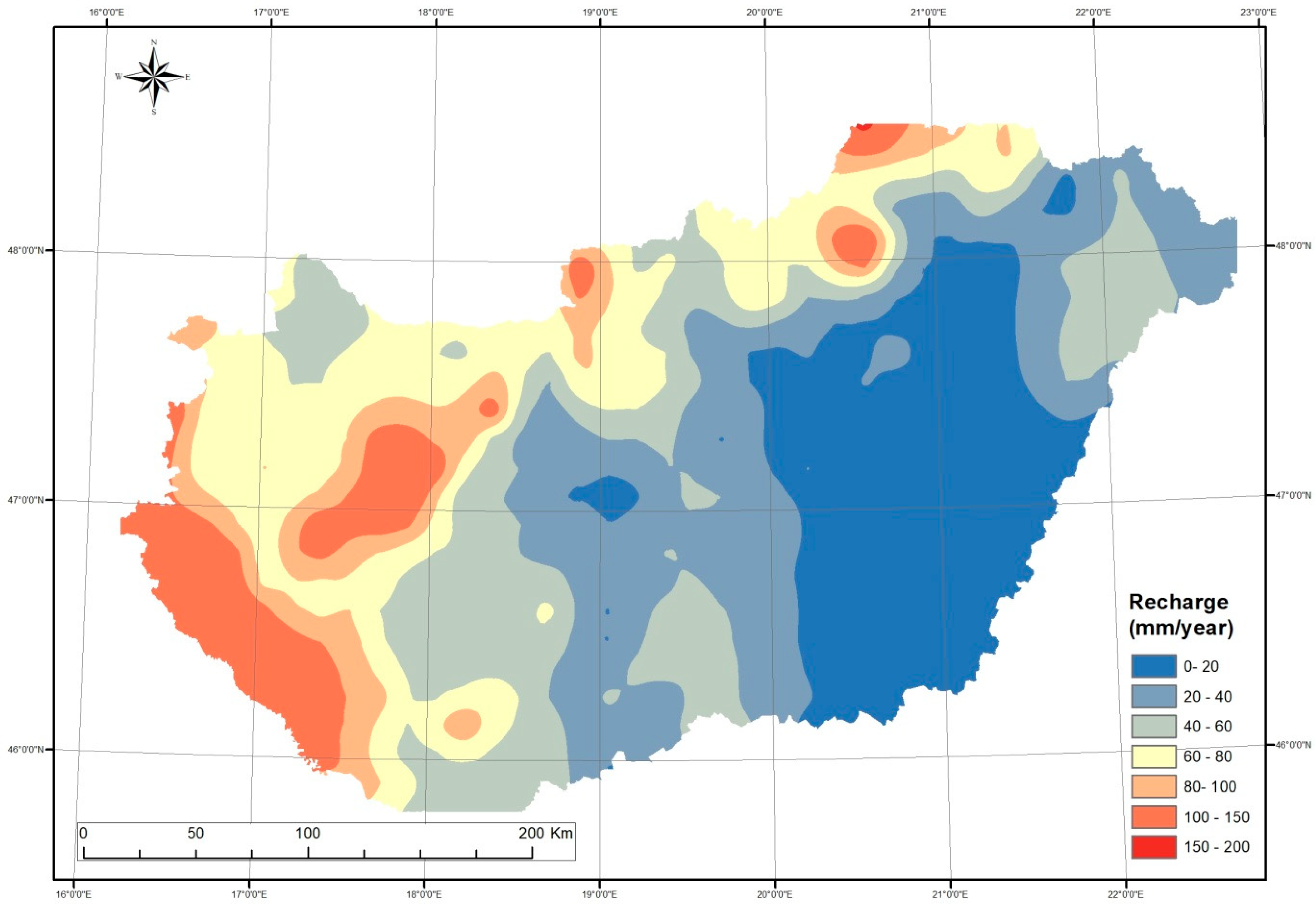
The distribution of averaged recharge for the 1961–1965 reference period is indicated in Figure 8.
Differences in recharge between the simulated time periods are indicated in Figure 9 and Figure 10. Simulation results indicate that recharge decreased by up to 50 mm/year between the early 1960s and the late 2000s in mountainous areas such as the Alpokalja area and the Northern Mountain Range. Slightly increasing recharge (by up to 20 mm/year) was simulated throughout the Great Hungarian Plain, the Mecsek Mountains and in the eastern part of the country.
Recharge calculations undertaken on ALADIN model results indicate decreasing recharge rates throughout the 21st century by up to 50 mm/y in the mountainous areas such as the Northern and Transdanubian Mountain Ranges and the Mecsek Mountains. These models do not predict recharge deficiency in the Alpokalja area, however slightly increasing recharge is predicted in parts of the Great Hungarian Plain and the Transdanubian Hills.
4.6. Groundwater Modelling
The goal of groundwater modelling was to simulate the water table distribution within the study area under various climate conditions. A two-dimensional steady state model was built for this purpose that was calibrated for transmissivity.
Modelling was performed with the USGS three-dimensional finite-difference ground-water model MODFLOW (MODFLOW-NWT). Calibration was performed with the model-independent parameter estimation code PEST and Beopest (version 17.05). Visual MODFLOW Flex was used as the graphical user interface during most of the modelling except for some of the calibration tasks.
For simplicity, in mountainous areas of open karst terrain, where shallow aquifers are absent, karst water table was simulated, and was considered to be hydraulically connected to adjacent shallow groundwater bodies. Model extent included the political borders of the country. The model domain was horizontally discretized into a rectangular grid with uniform cell sizes of 1000 m × 1000 m. Only one model layer was used extending from 0 m a.s.l. to the land surface elevation. Recharge as calculated and estimated according to the description presented earlier in this paper was selected as a boundary condition for the model at the upper boundary. Major rivers of Hungary and lakes with a surface area larger than 10 ha were selected as constant head internal boundary conditions for the model (Figure 11). Stream and lake stages were selected as the topographic elevation resulting in a slight overestimation of the water table elevation especially in the lowlands. This, however, does not have any negative impacts on our results as we were estimating changes instead of true heads and water table elevations.
Model calibration was performed using historical average water levels in 641 wells and 152 springs between 1961 and 1965. Wells and springs were selected to provide a relatively uniform coverage of the model area (Figure 11).
Water abstractions were not included in the model simulations. Simulated water table conditions are thus hypothetical distributions with the purpose of demonstrating the direct impacts of climate conditions rather than predicting actual future groundwater conditions.
As stated earlier, baseline conditions (natural-state) for the model were the average groundwater levels for the period of 1961–1965 as it can be reasonably assumed that compared with later periods, the shallow groundwater was not yet significantly affected by high industrial, agricultural, and residential water abstractions. This was confirmed by historical monitoring data series. Calibrated transmissivities obtained as a result of these assumptions were directly used for the simulation of the predictive scenarios.
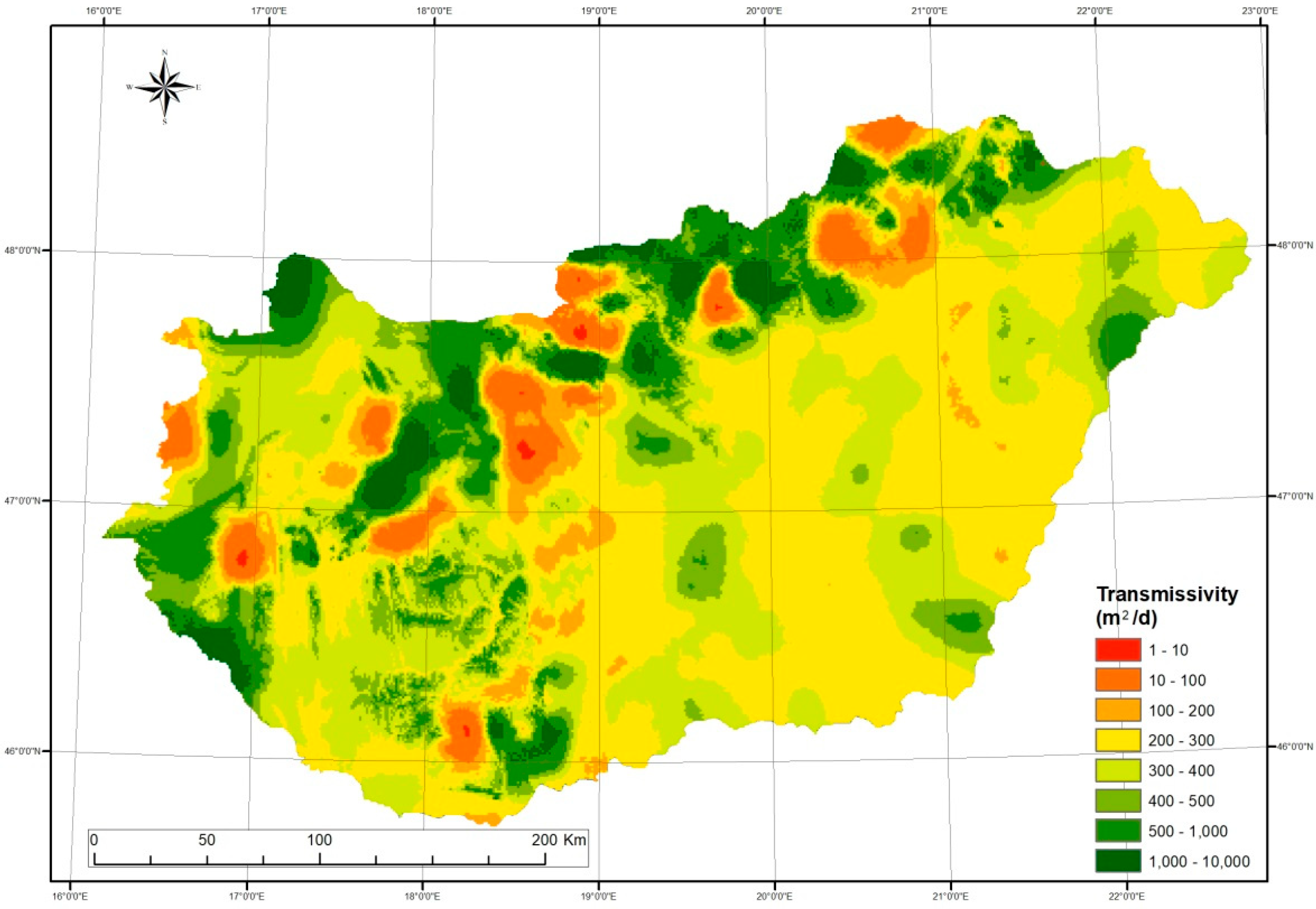
Due to the more-or-less arbitrarily chosen vertical model dimensions, calibrated hydraulic transmissivities do not have a direct physical meaning in terms of shallow aquifer properties, however, they provide information on the coupled impact of aquifer conductivity and aquifer thicknesses. The calibrated distribution of hydraulic transmissivity is shown in Figure 12. The calibrated transmissivities were qualitatively compared to known transmissivities at those locations where the model thickness approaches the true aquifer thickness the most, and found that the calibrated values at these locations are realistic.
Calibration Methodology
Model calibration was performed by means of manual and automated calibration using PEST. PEST [41] is a nonlinear parameter estimation code. Parameter optimisation is achieved using the Gauss–Marquardt–Levenberg method to drive the differences between model predictions and corresponding field data to a minimum in a weighted least squares sense. The implementation of this search algorithm in PEST is particularly robust; hence PEST can be used to estimate parameters for both simple and complex models including large numerical spatial models with distributed parameters.
The calibration process was restricted to the adjustment of hydraulic transmissivity until an acceptable match between calculated and measured water levels was obtained. Model calibration was undertaken with the assumption that field measured time-averaged water levels represent steady state (equilibrium) conditions of the groundwater system.
As a result of PEST calibration using pilot points, the resulting calibrated transmissivity field is spatially distributed. A number of 592 pilot points distributed over a regular mesh were used during the calibration process. Preferred homogeneity followed by preferred value Tikhonov regularization were used during the two-step calibration process. The total number of PEST calibration iterations resulting in the lowest measurement objective function was much larger (>25 iterations) than the number of iterations (7) after which the resulting transmissivity distribution was considered acceptable. After seven iterations the measurement objective function was lowered to an acceptable value (93248). The resulting mean value of non-zero weighted residuals was equal to −1.37.
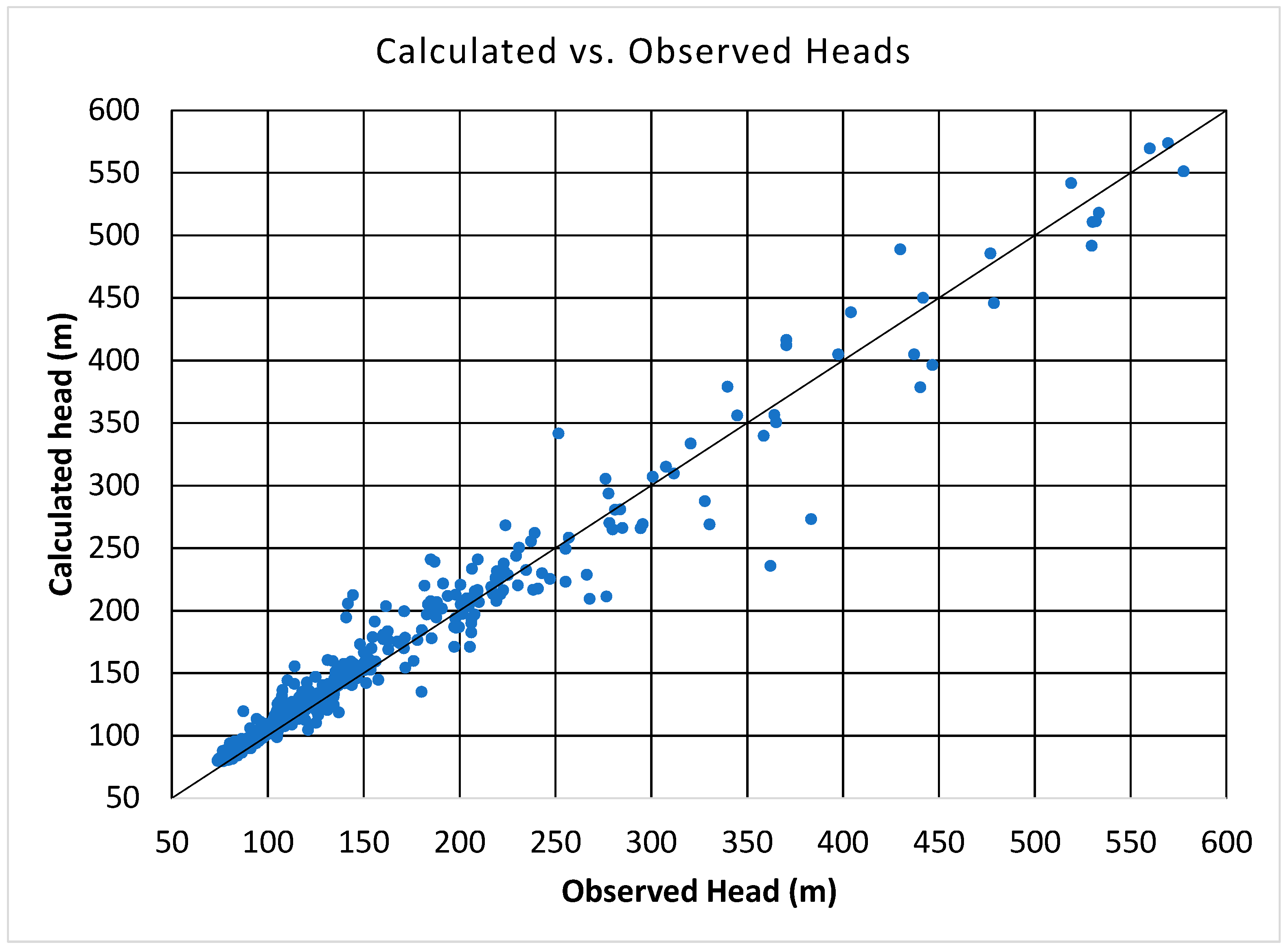
A slightly better fit (Figure 13) was achieved for the observation group consisting of springs than for the well observation group. While most upgradient dots in the calibration plot indicate locations with higher land surface elevation, wells are mainly located in the plain areas at lower elevations. This group can be identified as the dense cluster of points in the calibration plot within the downgradient section of Figure 13. The overall calibration seems satisfactory with an average discrepancy of slightly higher calculated heads than observed that was expected based on the selection of the boundary conditions. Calibrated water levels for 1961–1965 are presented in Figure 14.
5. Results
As stated above, shallow groundwater levels were first simulated for the period 1961–1965 that also served as the calibration period. Calculated (CARPATCLIM) climate parameters were used for the recharge estimates having been provided as input data for the simulation. Hydraulic properties (transmissivity) as calibrated during this simulation were used for the subsequent 1961–1990, 2021–2050, and 2071–2100 periods, and for which simulated (ALADIN) climate parameters were used as recharge estimates.
Simulated water table distribution for the 1961–1965 baseline period (Figure 15) and corresponding unsaturated zone thickness (depth to groundwater) presented in Figure 16 indicate that water table depth is generally very close to the ground surface in the lowlands such as the Alföld and Kisalföld areas and exceed depths of 100 m under mountain areas; although these values often correspond to karstwater bodies rather than shallow groundwater table, which might be perched above deep groundwater levels.
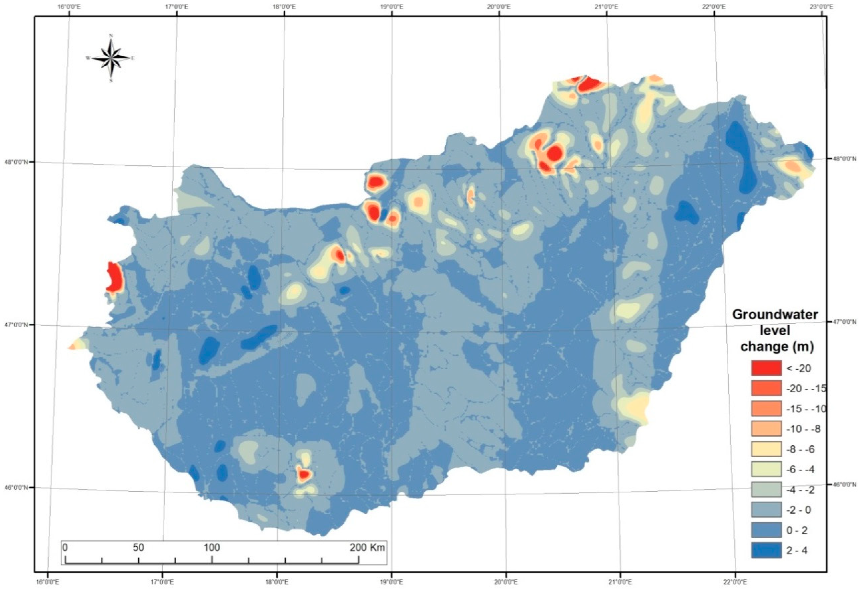
With the purpose of demonstrating the direct impacts of climate change on shallow groundwater resources, water table difference maps were constructed. The first of the three study periods (1961–1990) was considered as the reference period and the water table change calculated between this reference period and the 2021–2050 average water levels is presented on Figure 17.
This indicates significant water level drops (up to about -6 m with even higher drops at some places. The latter may also be attributed to less confidence in the simulated water levels at higher altitudes) under highland areas such as the Alpokalja, Eastern part of Transdanubian Mountains, Northern Mountain Ranges, and the Mecsek. A less significant decrease of groundwater levels was simulated along the southern reaches of the Tisza River (<−1 m) and the eastern parts of the Great Hungarian Plain (<−2 m). Most parts of the Transdanubian, the Kisalföld, the western parts of the Transdanubian Mountains, and the Duna-Tisza interfluve is characterized by increasing water levels, which exceed even 2 m at some locations.
The water table difference map (Figure 18) between the reference period (1961–1990) and the 2071–2100 averages indicates that the expected water level drops become slightly more significant at the same locations. Furthermore, the areas characterized by lowering water table elevations increase in size including some areas previously not being negatively affected such as the Duna-Tisza interfluve. The areas that previously were characterized as increasing water level zones become smaller in size and the expected water level increase was less significant.
6. Discussion
Several studies have been published about groundwater and climate change predicting changes in the water balance. Each of these studies apply climate data for their predictions, although different approaches were used for deriving climate data series [42]. Loaiciga et al. [43] used global averages. Allen et al. [44], Brouyere et al. [45], Vaccoro [46] applied regional projections for assessing climate change impacts. Scibek et al. [47] Jyrkama and Sykes [48], Serrat-Capdevila et al. [49], Toews and Allen [50] applied downscaled climate data in their investigations. Van Roosmalen et al. [51,52], Rosenberg at al. [53], York et al. [54] applied regional climate model projections in their studies.
The majority of early modelling studies employed stochastically generated daily weather series, and applied climate change shifts for predictive modelling. Many studies applied a range of global circulation models (GCMs) or used an averaged projection calculated from various GCMs. There are only a few studies that investigated the application of different downscaling methods.
Vaccoro [46] applied two different climate scenarios to investigate recharge sensitivity under various land use scenarios. This author also investigated the changes in recharge in response to the climate variability based on historical data. Rosenberg et al. [53] applied a Hydrologic Unit Model, imposed three GCMs and simulated the changes in water yields and groundwater recharge. Loaiciga et al. [43] used historical climate data from periods of draught, average and high precipitation. These authors scaled the historical time series to create climate change scenarios. This paper also evaluated the sensitivity of water resources at the aquifer scale through the combination of groundwater pumping scenarios with climate change scenarios. York et al. [54] utilized a coupled model of land and atmosphere and investigated climate change impacts on a watershed in Kansas, USA. Yu et al. [55] developed a novel methodology for interactive coupling of hydrologic models with climate models. Allen et al. [44] used shifted climate data using a stochastic weather generator. The differences were calculated based on three different GCMs and represented extreme climate conditions. This method was exploited in British Columbia, Canada. Brouyere et al. [45] extracted monthly precipitation and temperature from three GCMs in the Geer basin, Belgium. These authors calculated three future model scenarios by combining daily data with monthly change rates. These climate time series were used as inputs for an integrated model. Scibek et al. [47] used the estimates of aquifer recharge and runoff for the calculation of river discharges at the basin-scale. Jyrkama & Sykes [48] constructed various climate scenarios based on historical reference to model climate change impacts in southern Ontario, Canada. These authors calculated groundwater recharge using a distributive model. Serrat-Capdivela et al. [49] used downscaled results derived from an ensemble of GCMs and different IPCC scenarios. These authors determined spatially distributed recharge estimates from climate models. They applied a transient 3D integrated model to evaluate the hydrological conditions in the transboundary San Pedro Basin (US/Mexico). Van Roosmalen [51] used outputs from a regional climate model for two thirty-year periods and ran distributed hydrological model to simulate groundwater conditions in Denmark. Mileham et al. [56,57] harnessed a soil–water balance model to calculate water budget for several scenarios in Uganda. Rivald et al. [58] applied Regional Climate Model results as input for a catchment hydrological model (CATHY) for a catchment in Nova Scotia, Canada. Toews & Allen [50] investigated the sensitivity of recharge to climate projections of three different GCMs. These authors employed groundwater flow models for the simulation of groundwater levels in the Oliver Region in British Columbia. Tietjen et al. [59] exploited a model to investigate the dynamics of soil water under various climate conditions. Kidmose et al. [60] undertook a regional and local scale modelling study in Denmark while using the MIKE SHE integrated model environment. They applied extreme value analysis and used the ensemble approach. Raposo et al. [61] used the SWAT model to assess climate impact in Galicia-Costa, Spain. These authors utilized climate projections of various GCMs and evaluated two regional climate model scenarios. The study concluded that climate change has a significant influence on the temporal variability of recharge. Mollema & Antonelli [62] studied the seasonal variation of recharge to coastal aquifers. Potential evapotranspiration was estimated with the Thornthwaite method. The SEAWAT model was applied for simulating the influence of recharge on the size of freshwater lenses. Kumar [63] described a methodology for climate impact assessment including the downscaling of GCMs, the use of weather generators, simulation of recharge using rainfall-runoff models and calculation of groundwater conditions using MODFLOW.
Several additional studies have been published using approaches similar to those described above. Although the investigation techniques are improving, significant uncertainties are involved in climate predictions used as input parameters in climate impact assessment studies.
The simulation results achieved in this study were compared with climate impact studies undertaken in neighbouring countries. In a comprehensive study [64] the availability of water resources were analysed in 20 test areas across South East Europe (SEE region). Average climate conditions between 2021–2050 and 2071–2100 were analysed, based on regional climate model projections. Sensitivity of the different types of water resources to climate change was characterised based on the reactions of the hydrological system to changes of relevant meteorological parameters. Regional differences in the changes of water resources (recharge) were concluded to reflect the changes in precipitation and showed a clear geographical pattern. Most sites showed decreasing recharge and diminishing water resources. The test areas in the north and west showed significantly lower changes than those in the south and south-east of the SEE region. Decreases in recharge in the north and west are less than 10% until 2050 and do not exceed 20% until the end of the century. In the south and south-east of the SEE region the decrease is general and amounts to 10–40% in the first half of the century and 20–60% in the second half.
7. Conclusions
The present paper summarises a methodology developed for the calculation of groundwater table distributions from climate parameters. The goal of water table modelling was to develop a methodology that can be applied for the calculation of the water table under different climate conditions. This was done in order to facilitate climate impact assessment and the evaluation of climate sensitivity of groundwater aquifers.
We developed a modular approach to the quantitative investigation of the influence of climate conditions on groundwater table distribution:
- Climate zones were determined based on measured and simulated climate variables;
- Recharge zones were delineated based on slope, landuse and surface geology;
- Recharge was calculated for recharge zones making use of 1D analytical hydrological models;
- Groundwater table distribution was simulated using numerical groundwater models.
The interpolated daily climate datasets of the CARPATCLIM European database and the results of the ALADIN regional climate model were applied as input parameters in our modelling study. Climate zones were delineated quantitatively using the Thorntwaite methodology. Recharge zones (HRU’s) were delineated based on surface geology, landuse, and slope maps. We applied the HELP hydrological model for the calculation of recharge. The water table was calculated numerically using the MODFLOW numerical groundwater modelling code. The applied methodology provided a quantitative link between climate conditions and shallow groundwater conditions, in addition, it was successfully used for water table modelling.
The results of recharge calculation indicate that recharge decreased by up to 50 mm/year throughout the second half of the 20th century in mountainous areas such as the Alpokalja area, the Eastern section of the Transdanubian Mountains, and the Northern Mountain Ranges. Decreasing recharge rates of similar degree are predicted until 2100 in these areas and to a lower degree (up to 20 mm/y) in the Duna-Tisza Interfluve and Mecsek Mountain area (Figure 1 and Figure 10). Slightly increasing recharge rates (up to 20 mm/y) are predicted in the western part of the Transdanubian Mountains, and the Transdanubian Hills. Increasing recharge is a consequence of increasing annual rainfall in these areas, and also of the changing temporal pattern of rainfall.
Model predictions indicate decreasing water levels in highland areas such as the Alpokalja, Eastern Transdanubian Mountains, Mecsek, and Northern Mountain Ranges areas. The simulated water table drop can exceed 10 metres in certain locations, but it is generally less than 1 metre. Calculations based on climate model projections also indicate moderate water level drops in the Western part of the Tiszántúl area and the Duna-Tisza Interfluve, and the Szigetköz areas, which are generally less than 1 metre. Slightly rising groundwater levels (generally less than 3 metres) are predicted in the Transdanubian Hills, the western parts of the Transdanubian Mountains, and the Szamos Valley areas.
Climate change is predicted to have long-term influence on shallow groundwater resources. In large areas of the country, it is predicted to cause a moderate water table decline. This might impact surface waters, irrigation channels, and groundwater dependent ecosystems such as wetlands and riparian vegetation. Groundwater depletion also affects shallow groundwater uses such as dug wells. Groundwater level drops affect soil moisture conditions and can have adverse effects on natural vegetation and plant production. Furthermore, the significant decrease of annual rainfall over the eastern part of the country (up to 100 mm/y) is believed to cause additional indirect effects such as increased irrigational groundwater demand. This might cause additional pressure on groundwater resources and draws the attention to careful water resource management. In the western part of Transdanubia the projected increase of annual rainfall might facilitate a more effective use of groundwater resources.
Predictive simulations were based on climate simulations following the SRES A1B CO2 emission scenario. Future emission rates different from those assumed by the A1B scenario might entail different recharge rates and groundwater conditions in the future. The presented outputs were determined at the regional scale, and thus cannot be used for local-scale investigations. The presented methodology can be applied for modelling climate impacts at various scales for the assessment of climate vulnerability of groundwater resources.
Author Contributions
A.K. developed the methodology, performed analysis and modelling and prepared article. A.J. performed modelling and contributed to the article. All authors have read and agreed to the published version of the manuscript.
Funding
The research reported in this paper has been supported by the National Research Development and Innovation Office of Hungary (Grant No. TKP2020 BME-IKA-VIZ).
Institutional Review Board Statement
Not applicable.
Informed Consent Statement
Not applicable.
Data Availability Statement
Not applicable.
Conflicts of Interest
The authors declare no conflict of interest.
Disclaimer
Model results reflect the inaccuracies and uncertainties of the input databases. The methodology presented in this study makes the recalculation of model outputs possible making use of updated or completed datasets. The presented simulation results are representative at the country scale, and thus cannot be used for local-scale investigations. In order to increase the accuracy of the results, the resolution of the input datasets and applied models need to be increased.
References
- UNESCO. Groundwater Resources Assessment under the Pressures of Humanity and Climate Change (GRAPHIC): A Framework Document; GRAPHIC Series Number 2; United Nations Educational, Scientific, and Cultural Organization (UNESCO): Paris, France, 2008; p. 31. [Google Scholar]
- Hengeveld, H.G. Projections for Canada’s Climate Future. A Discussion of Recent Simulations with CGCM. Atmospheric and Climate Science Directorate, Science Assessment and Integration Branch; Meteorological Service Canada: Downsview, ON, Canada, 2000; 32p. [Google Scholar]
- Mearns, L.O.; Hulme, M.; Carter, T.R.; Leemans, R.; Lal, M.; Whetton, P. Climate scenario development. In Climate Change 2007: The Physical Science Basis. Contribution of Working Group I to the Fourth Assessment Report of the Intergovernmental Panel on Climate Change; Solomon, S., Qin, D., Manning, M., Chen, Z., Marquis, M., Averyt, K.B., Tignor, M., Miller, H.L., Eds.; Cambridge University Press: Cambridge, UK; New York, NY, USA, 2007; pp. 739–768. [Google Scholar]
- Le Treut, H.; Somerville, R.; Cubasch, U.; Ding, Y.; Mauritzen, C.; Mokssit, A.; Peterson, T.; Prather, M. Historical Overview of Climate Change. In Climate Change 2007: The Physical Science Basis. Contribution of Working Group I to the Fourth Assessment Report of the Intergovernmental Panel on Climate Change; Solomon, S.D.Q., Manning, M., Chen, Z., Marquis, M., Averyt, K.B., Tignor, M., Miller, H.L., Eds.; Cambridge University Press: Cambridge, UK; New York, NY, USA, 2007. [Google Scholar]
- Van Dijck, S.J.E.; Laouina, A.; Carvalho, A.V.; Loos, S.; Schipper, A.M.; Van der Kwast, H.; Nafaa, R.; Antari, M.; Rocha, A.; Borrego, C.; et al. Desertification in northern Morocco due to effects of climate change on groundwater recharge. In Desertification in the Mediterranean Region: A Security Issue; Kepner, W.G., Rubio, J.L., Mouat, D.A., Pedrazzini, F., Eds.; Springer: Dordrecht, The Netherlands, 2006; pp. 549–577. [Google Scholar]
- Woldeamlak, S.T.; Batelaan, O.; De Smedt, F. Effects of climate change on the groundwater system in the Grote-Nete catchment, Belgium. Hydrogeol. J. 2007, 15, 891–901. [Google Scholar] [CrossRef]
- Chiew, F.H.S.; McMahon, T.A. Modelling the impacts of climate change on Australian streamflow. Hydrol. Process. 2002, 16, 1235–1245. [Google Scholar] [CrossRef]
- Cayan, D.R.; Kammerdiener, S.A.; Dettinger, M.D.; Caprio, J.M.; Peterson, D.H. Changes in the onset of spring in the western United States. Bull. Am. Meteorol. Soc. 2001, 82, 399–415. [Google Scholar] [CrossRef] [Green Version]
- Stewart, I.T.; Cayan, D.R.; Dettinger, M.D. Changes in snowmelt runoff timing in western North America under a ‘business as usual’ climate change scenario. Clim. Change 2004, 62, 217–232. [Google Scholar] [CrossRef]
- Mote, P.W.; Hamlet, A.F.; Clark, M.P.; Lettenmaier, D.P. Declining mountain snowpack in western North America. Am. Meteorol. Soc. 2005, 86, 39–49. [Google Scholar] [CrossRef]
- Tague, C.; Grant, G.; Farrell, M.; Choate, J.; Jefferson, A. Deep groundwater mediates streamflow response to climate warming in the Oregon Cascades. Clim. Change 2008, 86, 189–210. [Google Scholar] [CrossRef]
- Barnett, T.P.; Pierce, D.W.; Hidalgo, H.G.; Bonfils, C.; Santer, B.D.; Das, T.; Bala, G.; Wood, A.W.; Nozawa, T.; Mirin, A.A.; et al. Human-induced changes in the hydrology of western United States. Science 2008, 319, 1080–1083. [Google Scholar] [CrossRef] [Green Version]
- Moberg, A.; Jones, P.D. Trends in indices for extremes in daily temperature and precipitation in central and western Europe, 1901–1999. Int. J. Climatol. 2005, 25, 1149–1171. [Google Scholar] [CrossRef]
- Spinoni, J.; Lakatos, M.; Szentimrey, T.; Bihari, Z.; Szalai, S.; Vogt, J.; Antofie, T. Heat and cold waves trends in the Carpathian Region from 1961 to 2010. Int. J. Climatol. 2015, 35, 4197–4209. [Google Scholar] [CrossRef] [Green Version]
- Illy, T.; Sábitz, J.; Szabó, P.; Szépszó, G.; Zsebeházi, G. A Klímamodellekből Levezethető Indikátorok Alkalmazási Lehetőségei; Országos Meteorológiai Szolgálat: Budapest, Hungary, 2015; 104p. [Google Scholar]
- Szentimrey, T.; Bihari, Z.T.; Lakatos, M.; Kovács, T.; Németh, Á.; Szalai, S.; Hiebl, J.; Auer, I.; Milkovid, J.; Zahradníček, P.; et al. Final Version of Gridded Datasets of All Harmonized and Spatially Interpolated Meteorological Parameters, per Country. Contract Number: OJEU 2010/S 110-166082. 2012. Available online: http://www.CARPATCLIM-eu.org/pages/deliverables.
- Thornthwaite, C.W. An approach toward a rational classification of climate. Geogr. Rev. 1948, XXXVIII, 55–93. [Google Scholar] [CrossRef]
- Schroeder, P.R.; Aziz, N.M.; Zappi, P.A. The Hydrologic Evaluation of Landfill Performance (HELP) Model: User’s Guide Version 3, EPA/600/R-94/168a; U.S Environmental Protection Agency Office of Research and Development: Washington, DC, USA, 1994.
- Gogolev, M.I. Assessing groundwater recharge with two unsaturated zone modeling technologies. Environ. Geol. 2002, 42, 248–258. [Google Scholar] [CrossRef]
- Kovács, A.; Marton, A.; Tóth, G.; Szőcs, T. A sekély felszín alatti vizek klímaérzékenységének országos léptékű vizsgálata. Hidrológiai Közlöny 2016, 9, 21–32. [Google Scholar]
- Lakatos, M.; Szentimrey, T.; Bihari, Z.; Szalai, S. Creation of a homogenized cli-mate database for the Carpathian region by applying the MASH procedure and the preliminary analysis of the data. Időjárás 2013, 117, 143–158. [Google Scholar]
- Szentimrey, T. Development of MASH homogenization procedure for daily data. In Proceedings of the Fifth Seminar for Homogenization and Quality Control in Climatological Databases, Budapest, Hungary, 29 May–2 June 2006; WCDMP-No. 71, WMO/TD-NO. 1493. pp. 123–130. [Google Scholar]
- Szentimrey, T.; Bihari, Z. Mathematical background of the spatial interpolation methods and the software MISH (Meteorological Interpolation based on Surface Homogenized Data Basis). In Proceedings of the Conference on Spatial Interpolation in Climatology and Meteorology; Szalai, Z.S., Bihari, T., Szentimrey, M., Lakatos, M., Eds.; COST Office: Luxemburg, 2007; pp. 17–28. ISBN 92-898-0033-X. [Google Scholar]
- Szalai, S.; Auer, I.; Hiebl, J.; Milkovich, J.; Radim, T.; Stepanek, P.; Zahradnicek, P.; Bihari, Z.; Lakatos, M.; Szentimrey, T.; et al. Climate of the Greater Carpathian Region; Final Technical Report; Carpatclim Consortium. 2013. Available online: www.carpatclim-eu.org.
- European Commission. Joint Research Centre, Carpatclim Database of the Carpathian Region; European Commission: Brussels, Belgium, 2013; Available online: http://www.carpatclim-eu.org.
- Hewitt, C.D.; Griggs, D.J. Ensembles based predictions of climate changes and their impacts. Eos Trans. AGU 2004, 85, 566. [Google Scholar] [CrossRef]
- Horányi, A.; Kertész, S.; Kullmann, L.; Radnóti, G. The ARPEGE/ALADIN mesoscale numerical modeling system and its application at the Hungarian Meteorological Service. Időjárás 2006, 110, 203–227. [Google Scholar]
- Bubnová, R.; Hello, G.; Bénard, P.; Geleyn, J.-F. Integration of the fully elastic equations cast in the hydrostatic pressure terrain-following coordinate in the framework of ARPEGE/Aladin NWP system. Mon. Weather Rev. 1995, 123, 515–535. [Google Scholar] [CrossRef] [Green Version]
- Météo-France Centre National de Recherches Météorologiques. ARPÉGE-Climate Version 5.1 Algorithmic Documentation; Météo-France: Paris, France, 2008. [Google Scholar]
- Farda, A.; Déqué, M.; Somot, S.; Horányi, A.; Spiridonov, V.; Tóth, H. Model ALADIN as regional climate model for central and eastern Europe. Studia Geophys. Geod. 2010, 54, 313–332. [Google Scholar] [CrossRef]
- National Adaptation Geo-information System of Hungary (NAGis). 2015. Available online: https://nater.mbfsz.gov.hu.
- Nakicenovic, N.; Swart, R. Special Report on Emissions Scenarios. A Special Report of Working Group III of the Intergovernmental Panel on Climate Change; Cambridge University Press: Cambridge, UK; New York, NY, USA, 2000. [Google Scholar]
- van Vuuren, D.P.; Carter, T.R. Climate and socio-economic scenarios for climate change research and assessment: Reconciling the new with the old. Climatic Change 2014, 122, 415–429. [Google Scholar] [CrossRef] [Green Version]
- Köppen, W. Das geographische System der Klimata. In Handbuch der Klimatologie; Köppen, W., Geiger, R., Eds.; Gebrüder Borntraeger: Berlin, Germany, 1936; 44p. [Google Scholar]
- Holdridge, L.R. Determination of world plant formations from simple climatic data. Science 1947, 105, 367–368. [Google Scholar] [CrossRef]
- Szelepcsényi, Z.; Breuer, H.; Ács, F.; Kozma, I. Biofizikai klímaklasszifikációk. 2. rész: Magyarországi alkalmazások. Légkör 2009, 54, 18–24. [Google Scholar]
- Ács, F.; Breuer, H. Biofizikai Éghajlat-Osztályozási Módszerek; ELTE University: Budapest, Hungary, 2012; 244p. [Google Scholar]
- Neitsch, S.L.; Arnold, J.G.; Kiniry, J.R.; Srinivasan, R.; Williams, J.R. Soil & Water Assessment Tool; Grassland, Soil & Water Research Laboratory: Temple, TX, USA, 2002.
- Gyalog, L.; Síkhegyi, F. (Eds.) Geological Map of Hungary, 1:100,000; Geological and Geophysical Institute of Hungary: Budapest, Hungary, 2005. [Google Scholar]
- European Environment Agency. Corine Land Cover Raster Data. 2006. Available online: http://www.eea.europa.eu/data-and-maps/data/corine-land-cover-2006-raster.
- John Doherty, PEST Model-Independent Parameter Estimation. In User Manual, 5th ed.; Watermark Numerical Computing: Brisbane, Australia, 2004.
- Green, T.R.; Taniguchi, M.; Kooi, H.; Gurdak, J.J.; Allen, D.M.; Hiscock, K.M.; Treidel, H.; Aureli, A. Beneath the surface of global change: Impacts of climate change on groundwater. J. Hydrol. 2011, 405, 532–560. [Google Scholar] [CrossRef] [Green Version]
- Loaiciga, H.A.; Maidment, D.R.; Valdes, J.B. Climate-change impacts in a regional karst aquifer, Texas, USA. J. Hydrol. 2000, 227, 173–194. [Google Scholar] [CrossRef]
- Allen, D.M.; Mackie, D.C.; Wei, M. Groundwater and climate change: A sensitivity analysis for the grand forks aquifer, southern British Columbia, Canada. Hydrogeol. J. 2004, 12, 270–290. [Google Scholar] [CrossRef]
- Brouyere, S.; Carabin, G.; Dassargues, A. Climate change impacts on groundwater resources: Modelled deficits in a chalky aquifer, Geer Basin, Belgium. Hydrogeol. J. 2004, 12, 123–134. [Google Scholar] [CrossRef] [Green Version]
- Vaccaro, J.J. Sensitivity of groundwater recharge estimates to climate variability and change, Columbia Plateau, Washington. J. Geophys. Res. 1992, 97, 2821–2833. [Google Scholar] [CrossRef]
- Scibek, J.; Allen, D.M.; Cannon, A.J.; Whitfield, P.H. Groundwater–surface water interaction under scenarios of climate change using a high-resolution transient groundwater model. J. Hydrol. 2007, 333, 165–181. [Google Scholar] [CrossRef]
- Jyrkama, M.I.; Sykes, J.F. The impact of climate change on spatially varying groundwater recharge in the grand river watershed (Ontario). J. Hydrol. 2007, 338, 237–250. [Google Scholar] [CrossRef]
- Serrat-Capdevila, A.; Valdes, J.B.; Perez, J.G.; Baird, K.; Mata, L.J.; MaddockIii, T. Modeling climate change impacts—And uncertainty—On the hydrology of a riparian system: The San Pedro Basin (Arizona/Sonora). J. Hydrol. 2007, 347, 48–66. [Google Scholar] [CrossRef]
- Toews, M.W.; Allen, D.M. Evaluating different GCMs for predicting spatial recharge in an irrigated arid region. J. Hydrol. 2009, 374, 265–281. [Google Scholar] [CrossRef]
- van Roosmalen, L.; Christensen, B.S.B.; Sonnenborg, T.O. Regional differences in climate change impacts on groundwater and stream discharge in Denmark. Vadose Zone J. 2007, 6, 554–571. [Google Scholar] [CrossRef]
- van Roosmalen, L.; Sonnenborg, T.O.; Jensen, K.H. Impact of climate and land use change on the hydrology of a large-scale agricultural catchment. Water Resour. Res. 2009, 45, W00A15. [Google Scholar] [CrossRef] [Green Version]
- Rosenberg, N.J.; Epstein, D.J.; Wang, D.; Vail, L.; Srinivasan, R.; Arnold, J.G. Possible impacts of global warming on the hydrology of the Ogallala Aquifer region. Clim. Change 1999, 42, 677–692. [Google Scholar] [CrossRef]
- York, J.P.; Person, M.; Gutowski, W.J.; Winter, T.C. Putting aquifers intoatmospheric simulation models: An example from the Mill Creek Watershed, northeastern Kansas. Adv. Water Resour. 2002, 25, 221–238. [Google Scholar] [CrossRef] [Green Version]
- Yu, Z.; Pollard, D.; Cheng, L. On continental-scale hydrologic simulations with a coupled hydrologic model. J. Hydrol. 2006, 331, 110–124. [Google Scholar] [CrossRef]
- Mileham, L.; Taylor, R.; Thompson, J.; Todd, M.; Tindimugaya, C. Impact ofrainfall distribution on the parameterisation of a soil-moisture balance model of groundwater recharge in equatorial Africa. J. Hydrol. 2008, 359, 46–58. [Google Scholar] [CrossRef]
- Mileham, L.; Taylor, R.G.; Todd, M.; Tindimugaya, C.; Thompson, J. The impact of climate change on groundwater recharge and runoff in a humid, equatorial catchment: Sensitivity of projections to rainfall intensity. Hydrol. Sci. J. 2009, 54, 727–738. [Google Scholar] [CrossRef] [Green Version]
- Rivard, C.; Paniconi, C.; Gauthier, M.J.; François, G.; Sulis, M.; Camporese, M.; Larocque, M.; Chaumont, D. A modeling study of climate change impacts on recharge and surface–groundwater interactions for the Thomas brook catchment (Annapolis Valley, Nova Scotia). In Proceedings of the GeoEdmonton, Canadian Geotechnical Society—International Association of Hydrogeologists—Canadian National Chapter Joint Annual Conference, Edmonton, AB, Canada, 21–24 September 2008. [Google Scholar]
- Tietjen, B.; Zehe, E.; Jeltsch, F. Simulating plant water availability in dry lands under climate change: A generic model of two soil layers. Water Resour. Res. 2009, 45, W01418. [Google Scholar] [CrossRef]
- Kidmose, J.; Refsgaard, J.C.; Troldborg, L.; Seaby, L.P.; Escriv, M.M. Climate change impact on groundwater levels: Ensemble modelling of extreme values. Hydrol. Earth Syst. Sci. 2013, 17, 1619–1634. [Google Scholar] [CrossRef] [Green Version]
- Raposo, J.R.; Dafonte, J.; Molinero, J. Assessing the impact of future climate change on groundwater recharge in Galicia-Costa, Spain. Hydrogeol. J. 2013, 21, 459–479. [Google Scholar] [CrossRef]
- Mollema, P.N.; Antonellini, M. Seasonal variation in natural recharge of coastal aquifers. Hydrogeol. J. 2013, 21, 787–797. [Google Scholar] [CrossRef]
- Kumar, C.P. AssessIng the impact of clImate change on groundwater resources. IWRA (India) J. 2016, 5, 3–11. [Google Scholar]
- Simonffy, Z. CC-WaterS—Climate Change and Impacts on Water Supply. WP4: Availability of Water Resources. Final Report. 2012. Available online: http://www.southeast-europe.net/en/achievements/outputs_library/?id=65.
Figure 1.
Main geographic regions of Hungary.

Figure 2.
Distribution of thirty-year average temperature for the period of 1961–1990 based on the CARPATCLIM database.
Figure 2.
Distribution of thirty-year average temperature for the period of 1961–1990 based on the CARPATCLIM database.

Figure 3.
Distribution of thirty-year average precipitation for the period of 1961–1990 based on the CARPATCLIM database.
Figure 3.
Distribution of thirty-year average precipitation for the period of 1961–1990 based on the CARPATCLIM database.
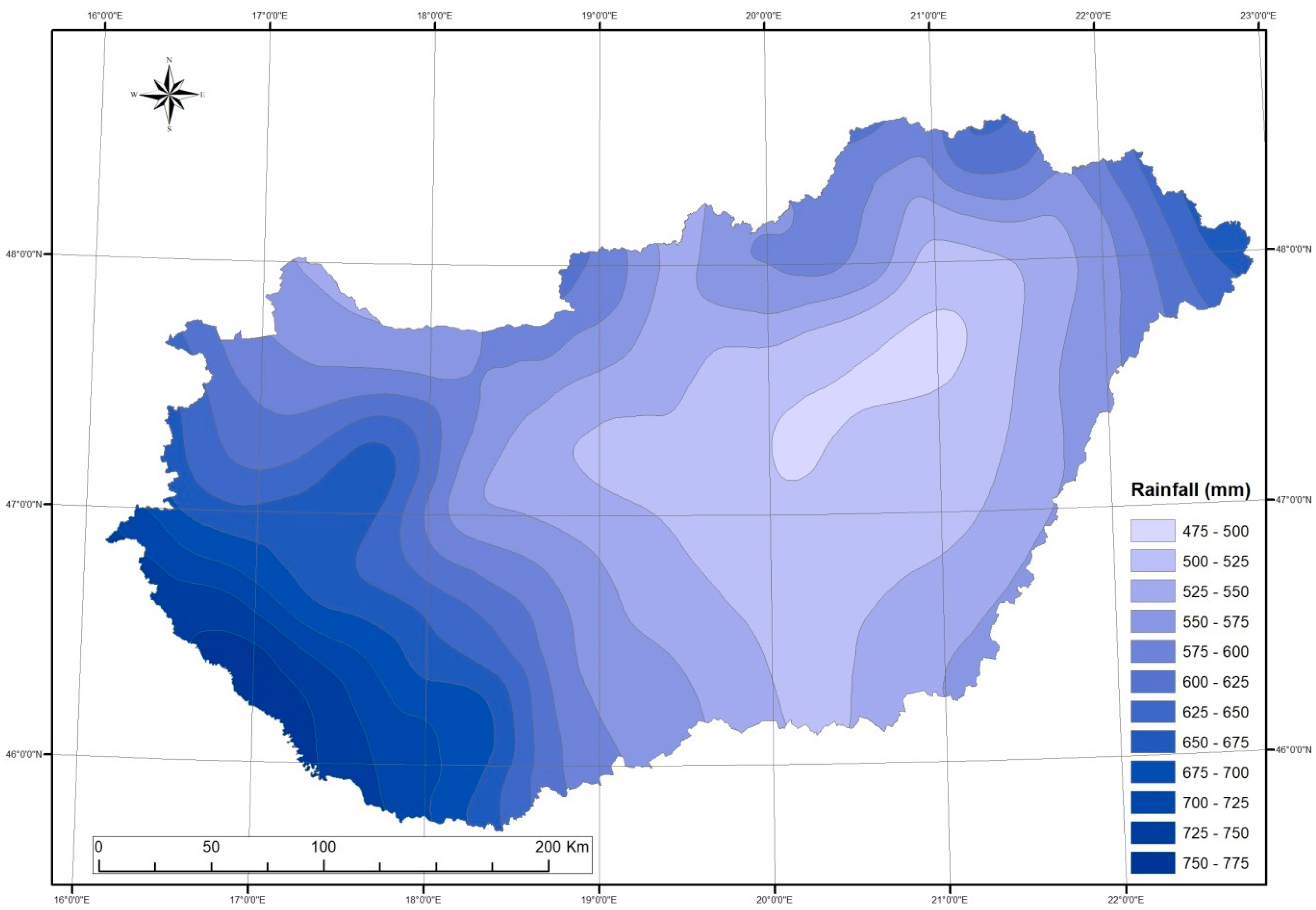
Figure 4.
Annual average temperature difference between the 1961–1990 and 2071–2100 periods based on ALADIN simulation results [15].
Figure 4.
Annual average temperature difference between the 1961–1990 and 2071–2100 periods based on ALADIN simulation results [15].

Figure 5.
Annual rainfall difference between the 1961–1990 and 2071–2100 periods based on ALADIN simulation results [15].
Figure 5.
Annual rainfall difference between the 1961–1990 and 2071–2100 periods based on ALADIN simulation results [15].
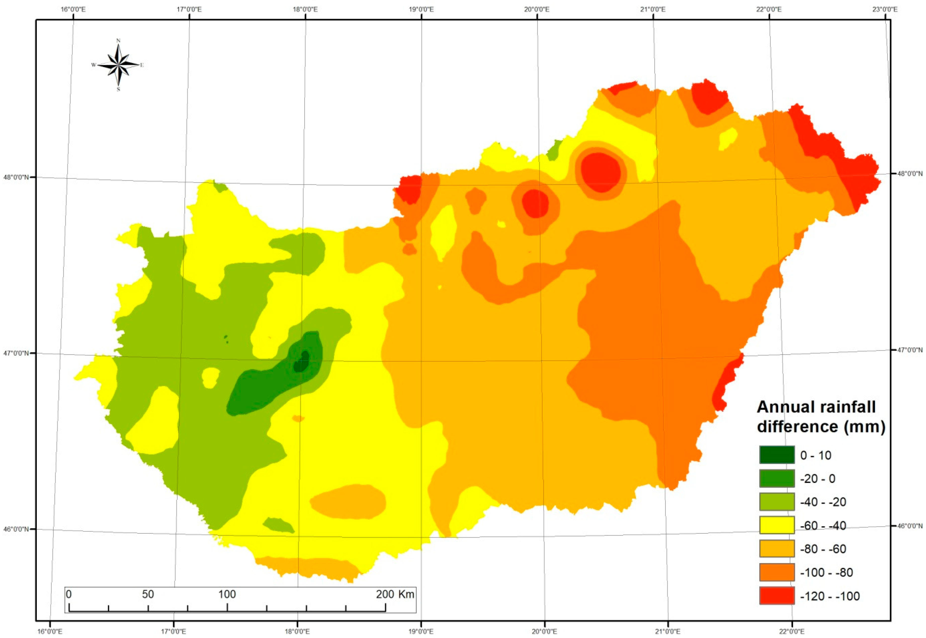
Figure 6.
Climate classification based on the Thorntwaite method for the period of 1961–1990 based on CARPATCLIM data. Numbers indicate climate zones.
Figure 6.
Climate classification based on the Thorntwaite method for the period of 1961–1990 based on CARPATCLIM data. Numbers indicate climate zones.
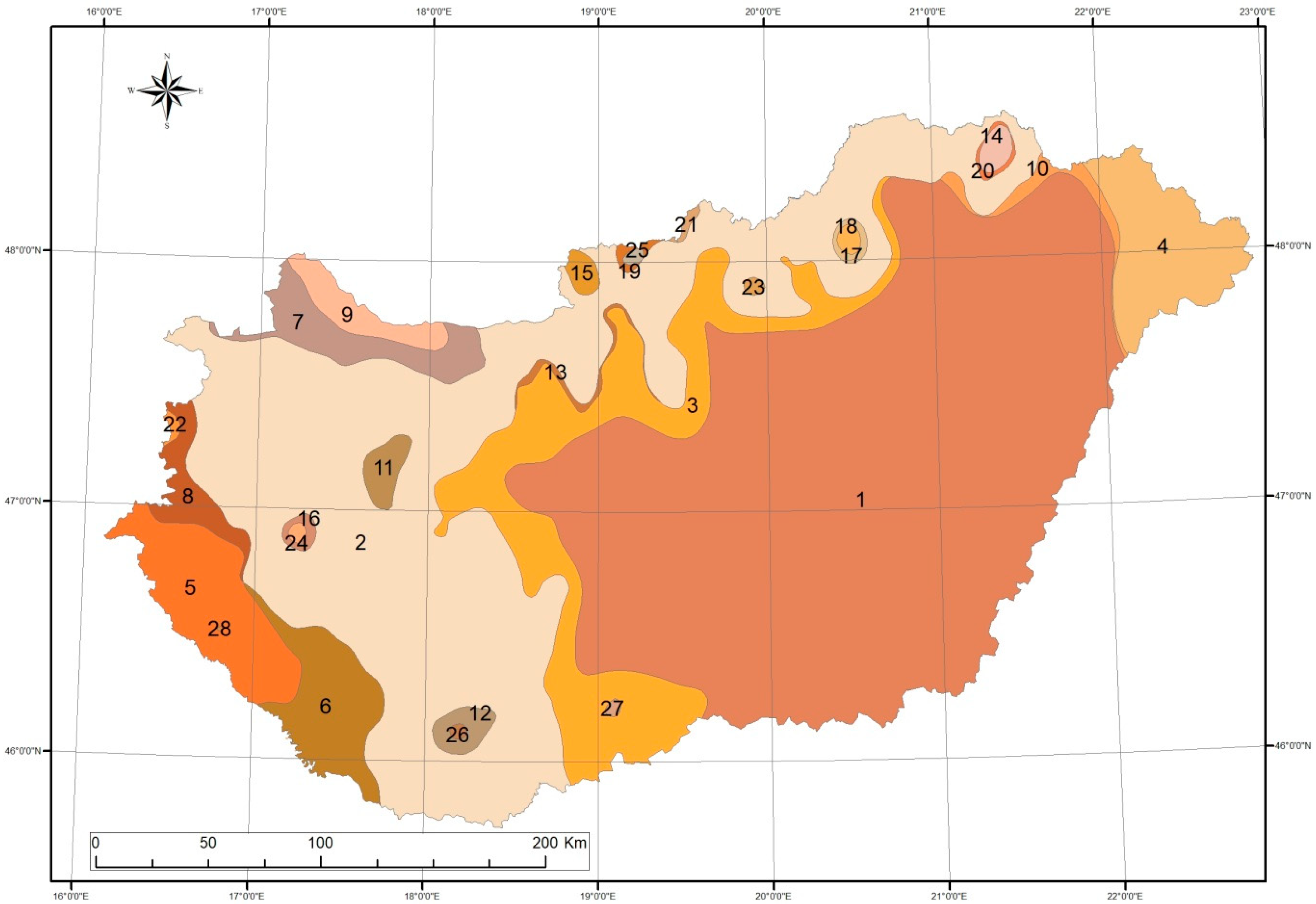
Figure 7.
Applied recharge zones delineated as a superposition of four data layers including climate zones, surface geology, landuse, and slope conditions. Different shades indicate different recharge characteristics.
Figure 7.
Applied recharge zones delineated as a superposition of four data layers including climate zones, surface geology, landuse, and slope conditions. Different shades indicate different recharge characteristics.
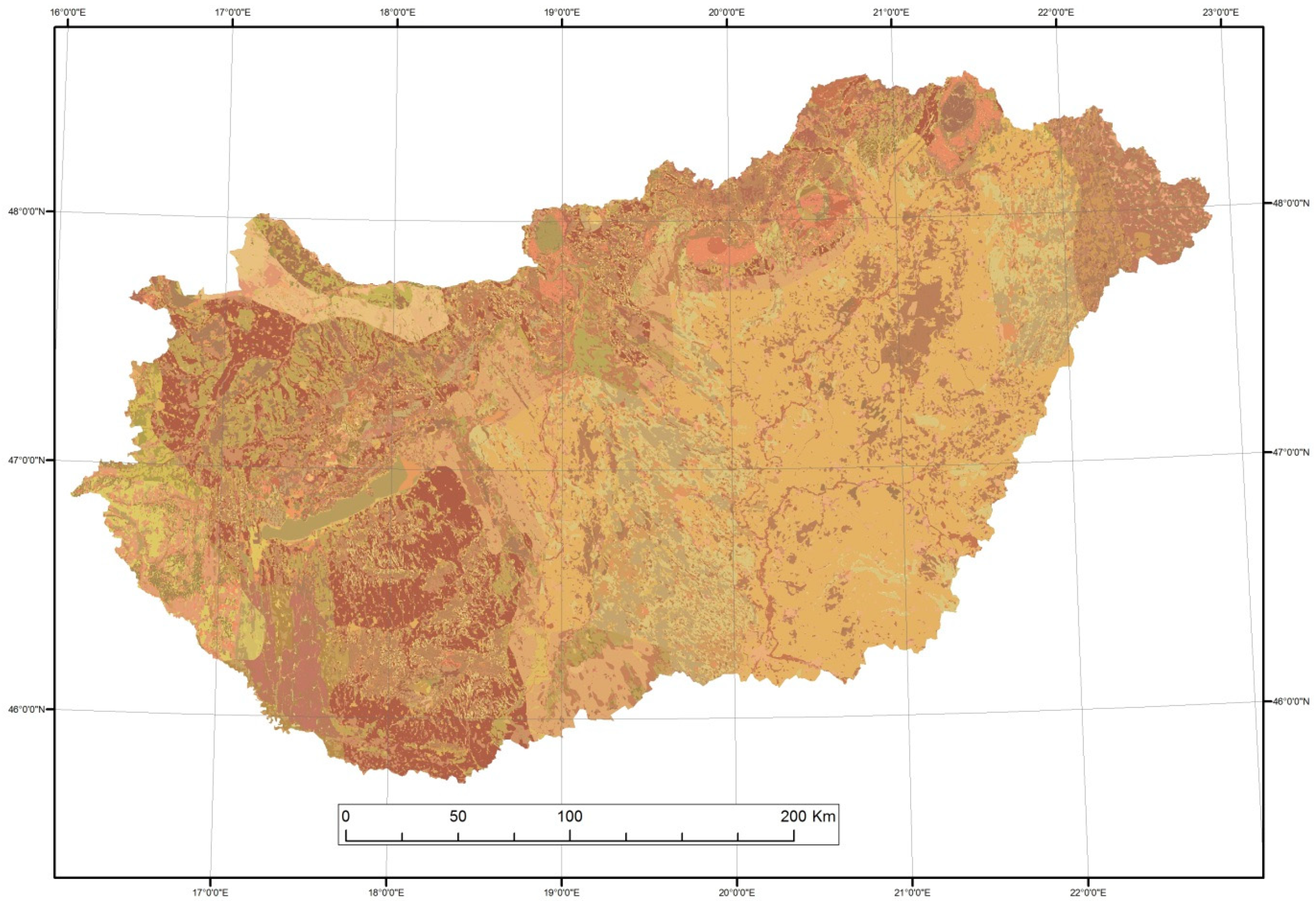
Figure 8.
Distribution of simulated recharge averaged between 1961 and 1965, based on CARPATCLIM dataset.
Figure 8.
Distribution of simulated recharge averaged between 1961 and 1965, based on CARPATCLIM dataset.

Figure 9.
Simulated difference in groundwater recharge between 2005–2009 and 1961–1965 averages based on CARPATCLIM data.
Figure 9.
Simulated difference in groundwater recharge between 2005–2009 and 1961–1965 averages based on CARPATCLIM data.
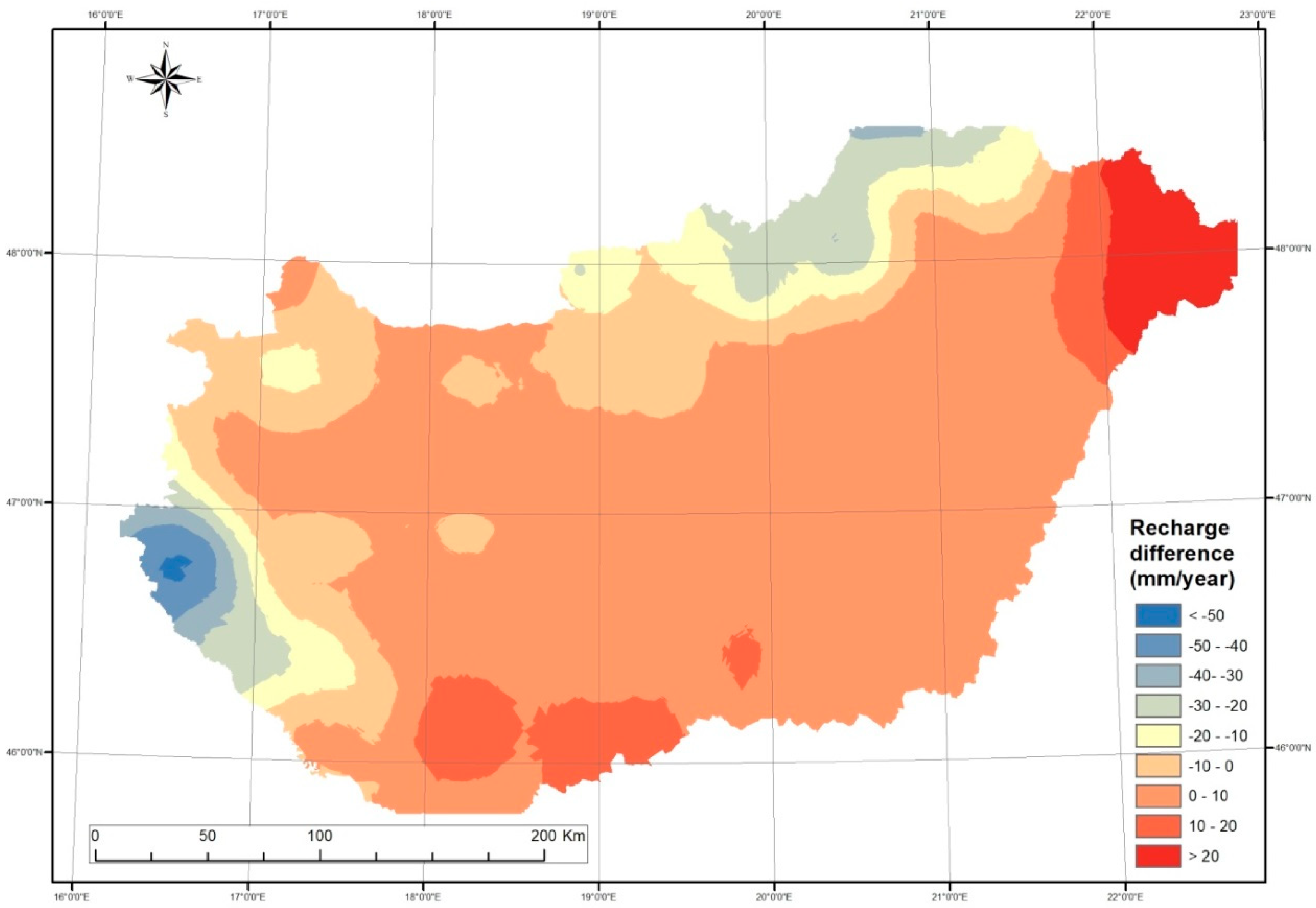
Figure 10.
Simulated difference in groundwater recharge between 2071–2100 and 1961–1990 averages based on ALADIN model results.
Figure 10.
Simulated difference in groundwater recharge between 2071–2100 and 1961–1990 averages based on ALADIN model results.
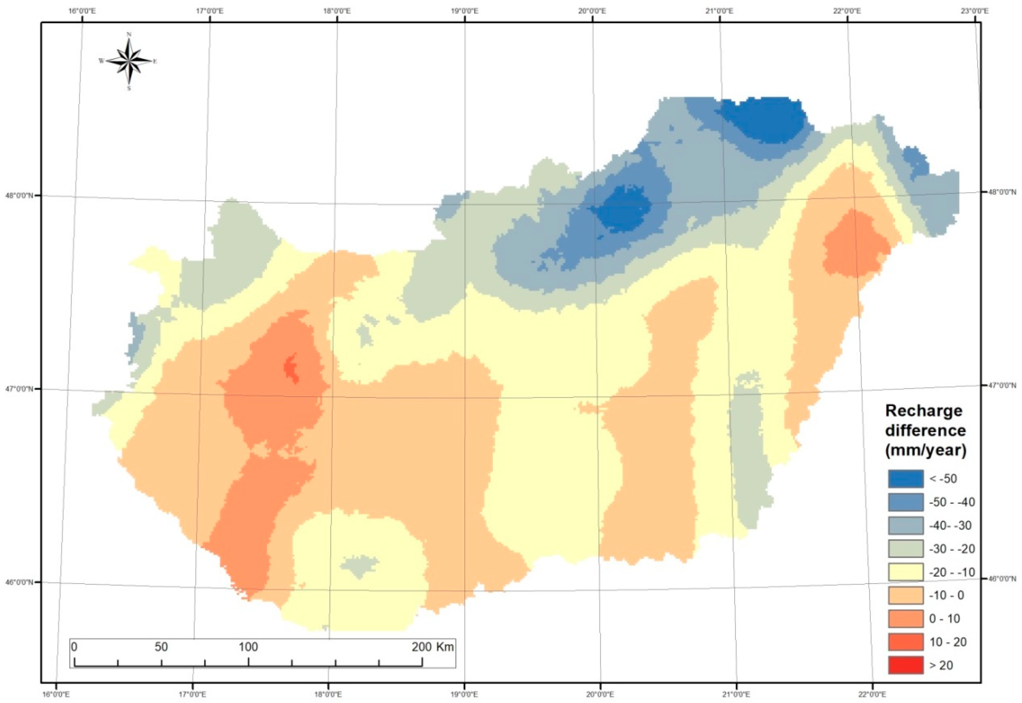
Figure 11.
Applied boundary conditions and calibration data points. Blue lines indicate rivers, green dots indicate monitoring bores and red dots indicate springs.
Figure 11.
Applied boundary conditions and calibration data points. Blue lines indicate rivers, green dots indicate monitoring bores and red dots indicate springs.
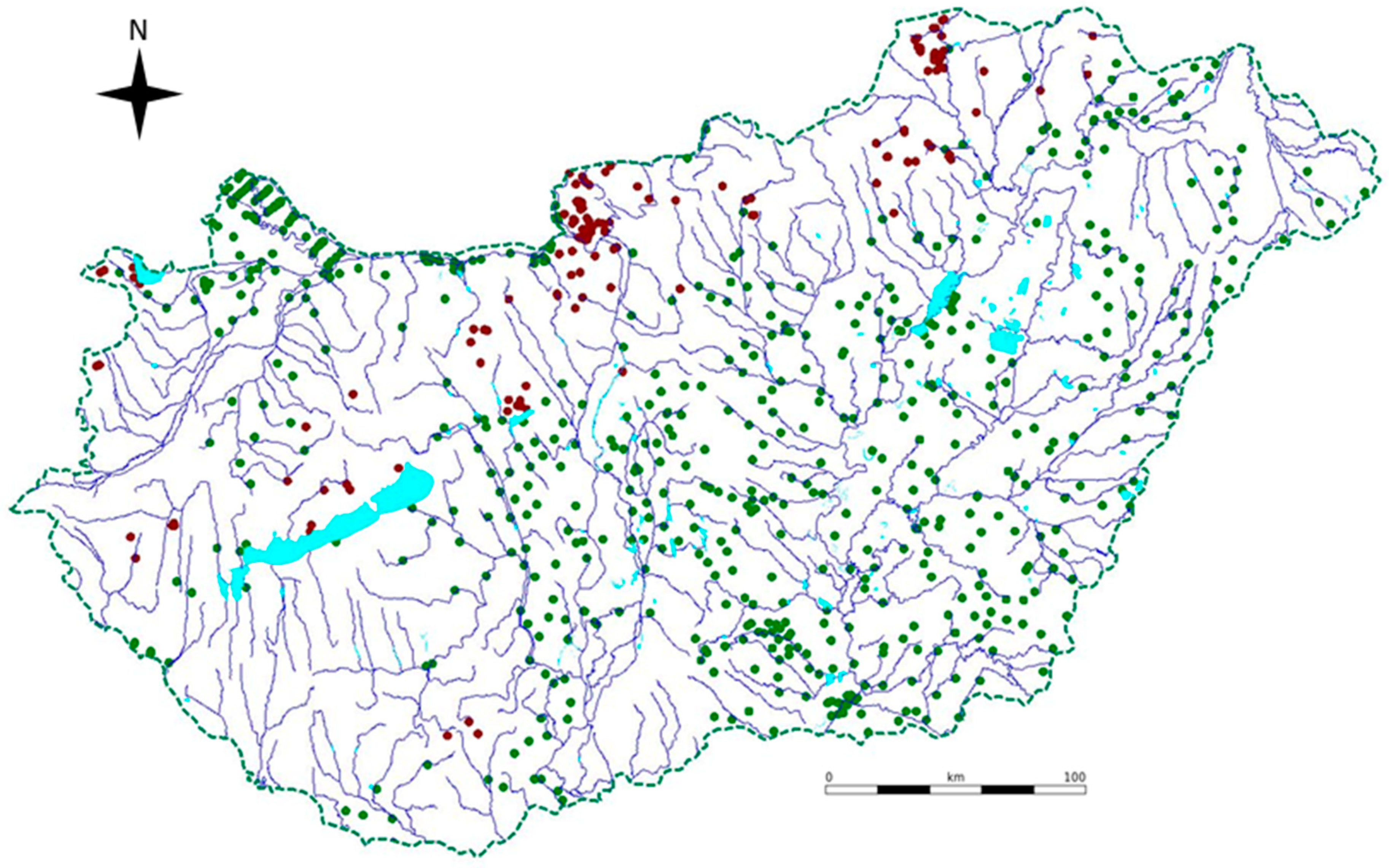
Figure 12.
Calibrated transmissivity distribution.

Figure 13.
Scatter plot of simulated vs. observed groundwater levels of the natural-state model.

Figure 14.
Simulated groundwater table: 1961–1965 average conditions. Green patches indicate unconfined karst areas.
Figure 14.
Simulated groundwater table: 1961–1965 average conditions. Green patches indicate unconfined karst areas.
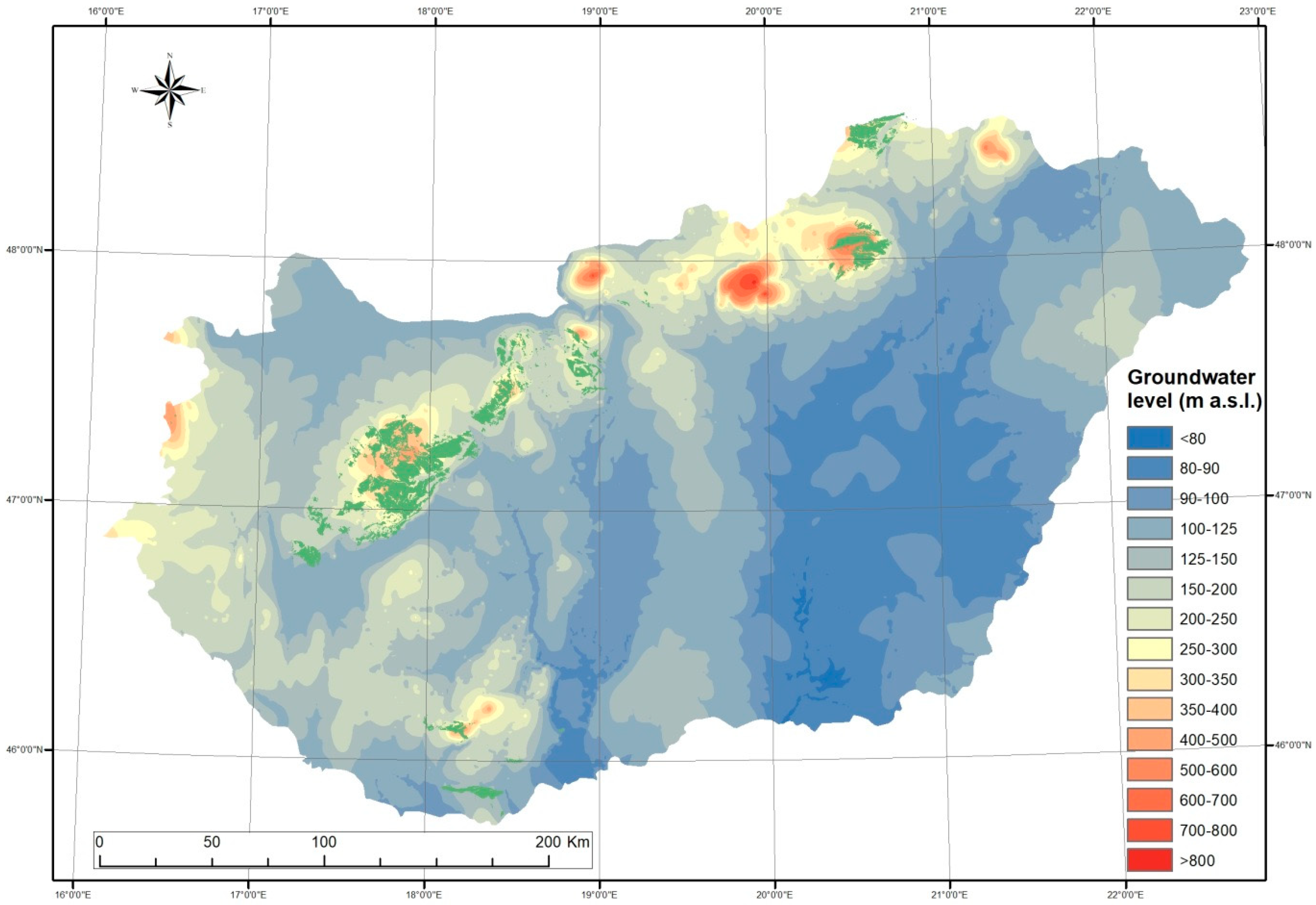
Figure 15.
Simulated groundwater table: 1961–1965 average conditions.
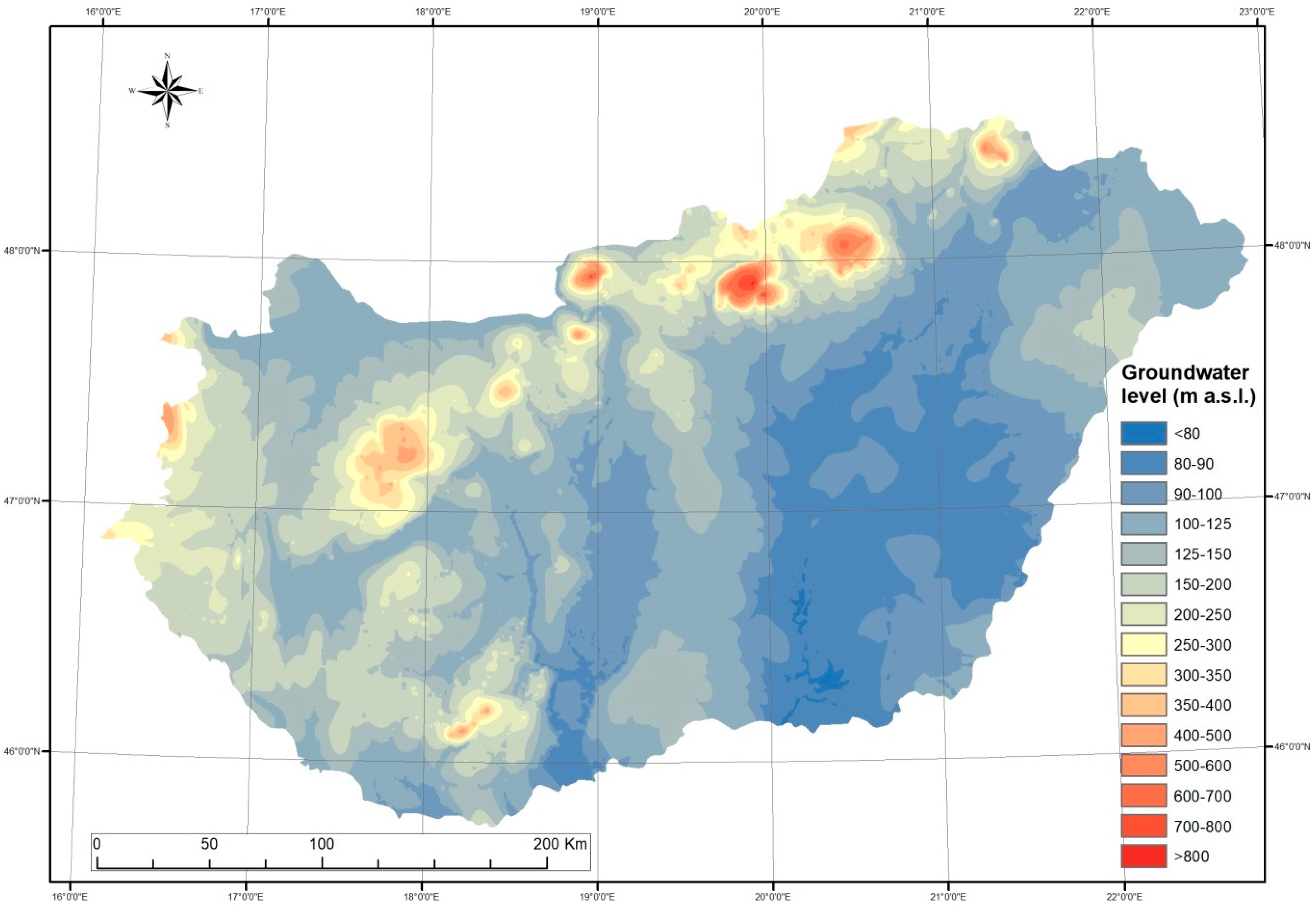
Figure 16.
Simulated unsaturated zone thickness map: 1961–1965 average conditions.
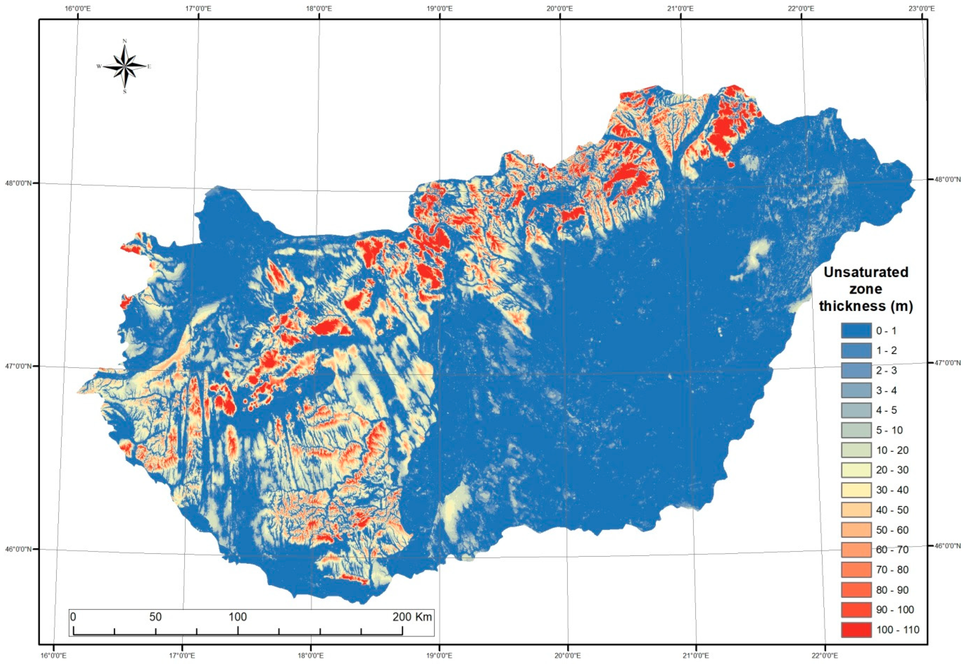
Figure 17.
Simulated difference in groundwater table between 2021–2050 and 1961–1990 averages based on ALADIN model results.
Figure 17.
Simulated difference in groundwater table between 2021–2050 and 1961–1990 averages based on ALADIN model results.
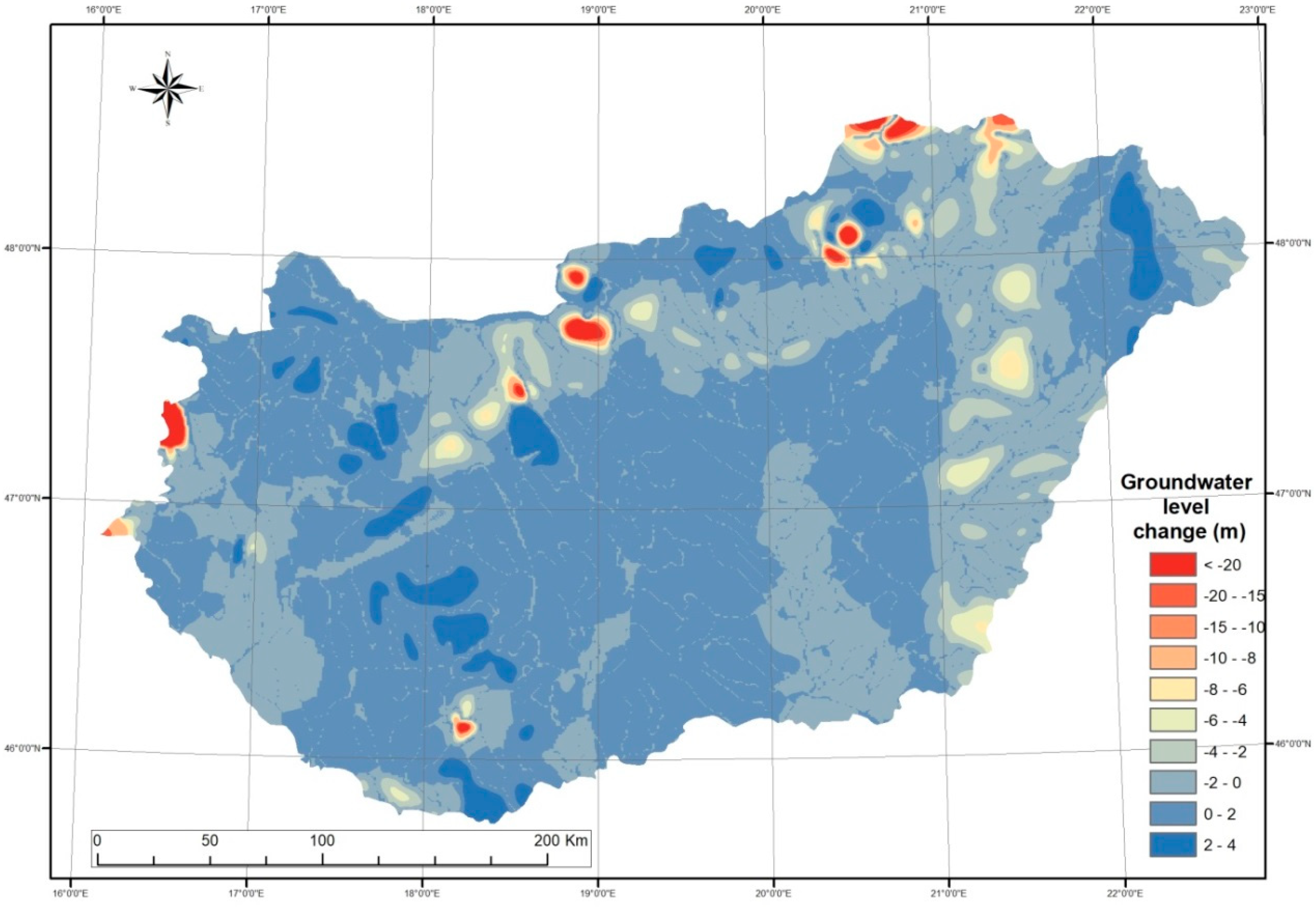
Figure 18.
Simulated difference in groundwater table between 2071–2100 and 1961–1990 averages based on ALADIN model results.
Figure 18.
Simulated difference in groundwater table between 2071–2100 and 1961–1990 averages based on ALADIN model results.

Publisher’s Note: MDPI stays neutral with regard to jurisdictional claims in published maps and institutional affiliations. |
© 2021 by the authors. Licensee MDPI, Basel, Switzerland. This article is an open access article distributed under the terms and conditions of the Creative Commons Attribution (CC BY) license (http://creativecommons.org/licenses/by/4.0/).
Share and Cite
MDPI and ACS Style
Kovács, A.; Jakab, A. Modelling the Impacts of Climate Change on Shallow Groundwater Conditions in Hungary. Water 2021, 13, 668. https://doi.org/10.3390/w13050668
AMA Style
Kovács A, Jakab A. Modelling the Impacts of Climate Change on Shallow Groundwater Conditions in Hungary. Water. 2021; 13(5):668. https://doi.org/10.3390/w13050668
Chicago/Turabian StyleKovács, Attila, and András Jakab. 2021. "Modelling the Impacts of Climate Change on Shallow Groundwater Conditions in Hungary" Water 13, no. 5: 668. https://doi.org/10.3390/w13050668
Note that from the first issue of 2016, this journal uses article numbers instead of page numbers. See further details here.