
Analysis of Unsteady Friction Models Used in Engineering Software for Water Hammer Analysis: Implementation Case in WANDA


1
Department of Environmental Engineering and Water Technology, IHE Delft Institute for Water Education, Westvest 7, 2611 AX Delft, The Netherlands
2
Department of Hydraulics for Infrastructure and Industry, Deltares, Boussinesqweg 1, 2629 HV Delft, The Netherlands
*
Authors to whom correspondence should be addressed.
Water 2021, 13(4), 495; https://doi.org/10.3390/w13040495
Submission received: 13 January 2021
/
Revised: 2 February 2021
/
Accepted: 9 February 2021
/
Published: 14 February 2021
(This article belongs to the Section Hydraulics and Hydrodynamics)
Abstract
:Transient events are frequent in water distribution systems. However, until now, most of the applications based on transient analyses are merely theoretical. Additionally, their implementation to real engineering problems is limited due to several physical phenomena accompanying transient waves, which are not accounted for in the classic approach, such as unsteady friction. This study investigates different unsteady friction models’ performance in terms of accuracy, efficiency, and reliability to determine the most-suited engineering practice. As a result of this comparison, Vítkovský’s unsteady friction model was found to be the best fit and was then implemented in WANDA commercial software. The implementation was verified with experimental data based on a reservoir–pipe–valve system. The model proved excellent performance; however, it was noticed that it fell short in simulating plastic pipes, where viscoelastic effects dominate. The upgraded software was then tested on different hydraulic networks with varying pipe materials and configurations. The model provided significant improvement to water hammer simulations with respect to wave shape, damping, and timing.
1. Introduction
Transient events are common in water distribution networks, usually leading to negative consequences such as water hammers [1]. Accordingly, problems such as pipe bursts and leakage frequently occur in water distribution networks [2,3]. In water distribution systems, the source of transient events may be related to valve maneuvers, pump trips, load acceptance, or rejection of turbines [4]. Therefore, researchers, water utilities, and engineers are interested in understanding the nature, generation, and propagation of water hammer waves [5,6,7].
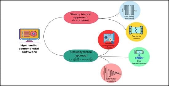
Several commercial software tools are available for the simulation of hydraulic transients and the design of hydraulic systems [8]. It was noticed that there are currently 21 available water hammer commercial software, as illustrated in Table 1. The majority of software (13 out of 21) use the methods of characteristics (MoC) to solve the hydraulic equation. Moreover, 18 out of the 21 software depends on steady/quasisteady friction models while computing water hammer equations. Out of the 21 software, three were only able to perform water hammer calculations based on the unsteady friction model. The Bentley Hammer, Hytran and TSNet Python package software used the Vítkovský friction model to analyze unsteady friction [8,9,10]. In contrast, WANDA, which is a software developed by Deltares Consultancy in the Netherlands, still uses quasisteady friction for hydraulic transient simulations and hydraulic system designs.
As mentioned in Table 1, currently available hydraulic commercial software can execute basic transient simulations. However, commercial software usually use a (quasi)steady friction assumption that notably affects the simulations’ quality [11]. Unsteady friction is among other dynamic phenomena that significantly affect transient behavior [12]. In contrast with steady friction, unsteady friction is dominant in the transient event’s later history [13]. Even though unsteady friction has remarkable effects on the hydraulic transients, it is rarely introduced in commercial hydraulic software. Hence, current commercial software cannot be adequately used for applications requiring a long and accurate estimation of the pressure waves, e.g., leakage detection.
Recently, many researchers have been encouraged to focus their research on the unsteadiness of friction in water hammers [13,14,15]. The underestimation of the dissipation, dispersion, and alteration of water hammer pressure waves in 1D models has been linked to unsteady friction [16]. Different experiments illustrated the importance of unsteady friction over steady friction, especially in fast transients [17,18]. Different approaches have been adopted to incorporate unsteady friction in transient flow simulation [19]. These methods can be classified into four categories [19]: (i) instantaneous mean flow velocity; (ii) instantaneous mean flow velocity and local acceleration; (iii) instantaneous mean flow velocity, local acceleration, and convective acceleration; and (iv) instantaneous mean flow velocity and past velocity changes weights.
Shamloo et al. [20] compared the numerical studies and experimental results done by Bergant and Simpson [21]. The models used were Brunone, Zielke, Vardy and Brown, and Trikha. They concluded that the results obtained from Brunone’s model seem to be overestimated for laminar flow than the other unsteady models. The models of Zielke, Vardy and Brown, and Trikha have similar results, where the maximum heads and wave shape are accurately predicted. Another comparison was performed by Jensen et al. [22], who compared different models (steady, quasisteady, Brunone, Vardy and Brown, Zielke) with experimental data performed by Soares et al. [23]. This study showed that Brunone’s model provided better results over steady and quasisteady friction models. In contrast, convolution-based models (Zielke and Vardy and Brown) provided the most accurate results. The results illustrated that there is no need to enhance the model from steady friction to quasisteady friction as the improvement of accuracy is almost negligible, and the focus for improvement falls into the unsteady friction approach.
This study aims to fill the gap between academia and the hydraulic software industry in terms of implementing the most-suited unsteady friction model for engineering practice in hydraulic commercial software. Different unsteady friction models were compared, and the most suitable model was chosen to be implemented in WANDA based on well-developed criteria. The upgraded WANDA software with the unsteady friction model was tested on different hydraulic networks to illustrate the newly acquired attributes. Moreover, the recently implemented WANDA software was compared to other commercial software, including the Bentley Hammer and TSNet Python package, which also assumes unsteady friction computation. The main outcome of this study is to provide commercial software with more accurate transient solvers by means of adding unsteady friction, providing a framework to carry out analysis such as inverse transient analysis, which aims to solve standard engineering problems such as leakage detection.
2. Methodology
2.1. Implementation of the Hydraulic Solver
The method of characteristics was used to solve the water hammer hyperbolic differential equation due to its computational efficiency, accuracy, and ease of programming [4]. The classic water hammer model has been implemented in Python based on the MoC, solving Equations (1)–(3),
where (R) is the convenient coefficient, (Q) is the flow, (g) is acceleration due to gravity, (t) is time, (a) is the wave celerity, (D) is the diameter, and (A) is the Area. The friction (f) is the summation of the quasisteady friction (fq) and unsteady friction (fu)
In this section, several friction models were implemented using the equations illustrated in Table 2. The implemented models were quasisteady friction and unsteady friction models. Generally, steady friction assumes that the friction factor f is constant along with the simulation. However, the quasisteady friction assumption assumes that the Reynolds number is calculated and updated at each new computation as shown in Equation (5).
Four different categories of unsteady friction models were implemented, including (i) instantaneous mean flow velocity; (ii) instantaneous mean flow velocity and local acceleration; (iii) instantaneous mean flow velocity, local acceleration, and convective acceleration; (iv) and instantaneous mean flow velocity and past velocity changes weights.
Hino is the most common instantaneous mean flow velocity unsteady friction model. The model is only function of instantaneous mean flow velocity. This model was implemented using Equation (6). The unsteady friction term was added to the quasisteady friction forming the overall friction at each new computation. Daily’s model was implemented using Equation (7). To compute Daily’s model, prior knowledge of the steady friction component is needed. Furthermore, the finite difference was used to calculate the local acceleration (). Brunone’s model is dependent on instantaneous acceleration, instantaneous convective acceleration and a damping coefficient as illustrated in Equation (8). Vítkovský’s model is similar to Brunone’s model. However, it has an additional sign term, which provides the right sign for the convection term for all potential flows, acceleration, or deceleration phases, as illustrated in Equation (9). Explicit first-order finite differences were used to calculate local acceleration () and convective acceleration (). Instantaneous mean flow velocity and past velocity changes weights unsteady friction models are usually solved using convolution equations as illustrated in Equation (10). The convolution was solved with a regular rectangular grid with first-order finite-difference approximation. In this paper, the Vardy and Brown weighting function was used as demonstrated by Equation (11). In terms of model analysis, it is expected that Hino’s model would require the least computational requirements due to the simpler modeling assumptions (instantaneous mean flow velocity); however, accuracy is expected to be lower. On the other hand, Vardy and Brown would provide the highest accuracy but the highest computational efforts due to more complex assumptions, involving convolution of past velocity changes. For Brunone, and Vítkovský, the models are expected to have moderate computational requirements as they are dependent on instantaneous mean flow velocity, local and convective accelerations.”
2.2. Validation with Experimental Data
The implemented water hammer models were validated by means of experimental data, which were collected as part of the water hammer test series in the copper straight pipe facility, assembled at the Laboratory of Hydraulics and Environment of Instituto Superior Técnico (LHE/IST) and presented in Ferràs et al. [19]. The pipe rig consisted of a reservoir–pipe–valve system, and pressure histories were recorded at different pipe sections. The system comprises a 15.49 m long pipe, inner diameter D = 0.020 m, pipe wall thickness e = 0.0010 m, and a Young modulus of elasticity of E = 105 GPa. High-quality pressure transducers (WIKA S-10) were used for the pressure data acquisition at a frequency of 600 Hz.
Regarding the experiment conditions, the flow used was Qin = 4.2 L/min, with a wave celerity (c) of 1239 m/s, while the effective valve closure time (tv) was 0.003 s. The initial head at the reservoir (Hres) was 54.2 m.
2.3. Comparison of Friction Models
The following criteria were followed to assess the unsteady friction models in the Python environment that can fit in commercial software:
- i.
- User input requirements
- ii.
- Stability of the model
- iii.
- Computational efficiency
- iv.
- Model accuracy
2.3.1. Input Requirements and Stability
Each model’s input requirements were analyzed to ensure that users do not need to have prior information to use any of the friction models. Hence, models that are dependent on user’s inputs were not favored to be implemented in commercial software, while robust models that do not require user’s inputs were favored.
The stability was checked qualitatively over short and long simulation periods to ensure that the models were running as expected without numerical instabilities.
2.3.2. Computational Efficiency
Execution time is a matter of interest for any software developer. To analyze such an aspect efficiently, the trends concerning a particular factor are the matter of interest rather than absolute values. Hence, the growth of execution time relative to the input is the concern.
Big O notation is one of the most common notations related to task size and the computational resources requirements. The Big O notation represents the trend of execution time in order (O) of a function (g(n)).
The computational efforts analysis was performed using a set of input time simulation period arrays for different friction model simulations. The execution time was tracked for each simulation period. The retrieved simulation period and execution time data were fitted, and the dominant term was determined for each friction model using Equation (12).
2.3.3. Accuracy Comparison
The accuracy comparison was performed by comparing the simulated friction models’ peaks and comparing it with the real measurement data. This means of comparison has been commonly applied in literature for comparing the accuracy of the friction models [21,22,30]. The summation of square error (SSE) demonstrated in Equation (13) has also been used to assist the error calculation.
where Hm is the measured head, and Hsim is the simulated head.
2.3.4. Weighted Average Comparison
To assess the final chosen model, a weighted average matrix was used to compare between the models based on different criteria. A score out of 10 was given to each criterion. However, each criterion was given a different weight. For example, user input requirements and stability were given a weight of 1 each as most of the models were stable and did not need an input. However, accuracy and time computation were given a weight of 3 due to their significant importance.
2.4. Application
The most-suited unsteady friction was incorporated in WANDA’s environment. The unsteady friction was calculated and added to the quasisteady friction component at each computation time step, as illustrated in Equation (3).
The WANDA software with the implemented new model was verified using the same experimental data stated in Section 2.1. Additionally, WANDA was compared with the most-suited unsteady friction in the Python model. Hence, a comparison of WANDA’s and the developed Python’s code would be enough for the verification.
A simple synthetic network was constructed to easily compare the effects of transient event simulation at the valve using unsteady friction with the previously installed quasisteady friction model. The network is composed of an elevated tank, 5 pipes, 2 nodes, a butterfly valve, and the final reservoir. The network is illustrated in Figure 1. Specifications of the network can be found in Table 3.
At the same experiment, the effects of different pipe materials on the transient event simulated at the valve were studied. The pipes had different Young modulus values, as illustrated in Table 4.
In these experiments, the valve closure was adjusted to be totally closed within 1 s, starting from 5.29 to 6.29.
2.5. Comparison of WANDA with Available Commercial Software
Upon checking the scientific literature, it was found that there are currently three commercial software capable of doing the hydraulic simulation using an unsteady friction model. The three software are the Bentley Hammer (Bentley Systems, Exton, PA, USA), Hytran (University of Auckland, Auckland, New Zealand) and TSNet (University of Texas at Austin, Austin, TX, USA) package. All software are using Vítkovský’s friction. Hence, comparing the upgraded WANDA with those software would give precious insights into its current capabilities and performance.
3. Results and Discussion
3.1. Comparison of Friction Models
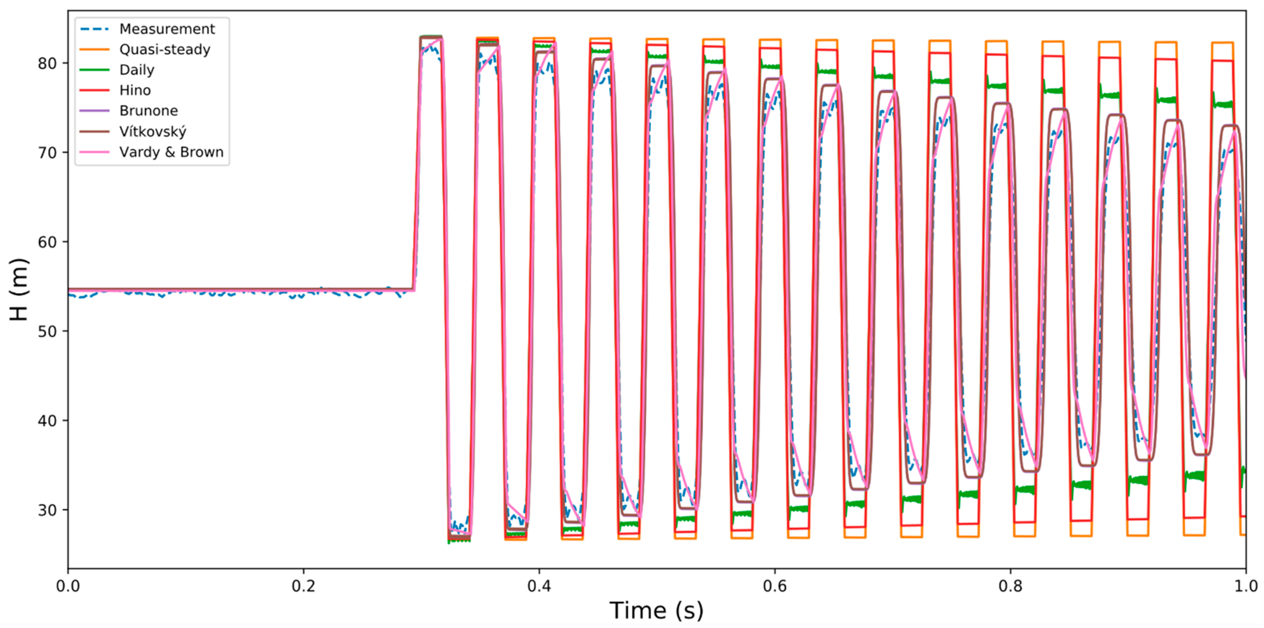
The quasisteady friction simulation was conducted and compared to the experimental results obtained. The obtained simulation of the head is shown in Figure 3. As illustrated in Figure 3, the quasisteady friction gives a reasonable estimation of the first peak; however, it overestimates the later oscillation peaks compared to the real experiment, where significant damping occurs due to the unsteady friction among other dynamic phenomena. The underestimated damping was also observed in the experimental results of Shamloo et al. [20], Twyman [31], and Cao et al. [11], which indicates the steady and quasisteady friction’s inability to model frequency-dependent attenuation [17].
As illustrated by Figure 3, a slight improvement can be noticed by Hino’s model simulation over the steady and quasisteady friction simulations. Hino’s model’s later oscillations are less overestimated than the prementioned models, and the wave attenuation is slightly better than the quasisteady model. However, the overall quality of the model is still weak, especially for measuring the later oscillations. These observations have been mentioned before by several studies as well [30]. Regarding Daily’s model, it was noticed that the damping in this model was higher than the previous models; this is mainly attributed to the local acceleration component, which makes the simulation more accurate. As demonstrated in Figure 3, Brunone’s model and Vítkovský’s model show a significant improvement over the previous unsteady friction models and illustrate that the unsteady friction dominates over the steady friction [17]. Vítkovský’s model provides slightly more accurate results than Brunone’s as it has the sign correction term [32]. Brunone and Vítkovský’s friction models have been implemented by different authors who reported similar results of high accuracy than the previously implemented friction models [22,23,33]. Vardy and Brown’s model provided the best damping and wave attenuation results compared to the previously mentioned models [22]. This is attributed to the high accuracy of the convolutional-based unsteady friction models.
3.1.1. Input Requirements and Stability
All models can work independently, except Daily’s model, which might need an adjustment of a factor by the user depending on the case. Hence, this model showed an unstable behavior in its peaks, which is clearly demonstrated by spike noises that develop on time. Different experiments were conducted, leading to different constants [25,34,35]. Hence, this friction model might not be suitable for the direct use of all hydraulic setups.
3.1.2. Computational Efforts Requirements
A time complexity analysis was performed according to the methodology illustrated in Section 2.2, and the following results were obtained, as shown in Table 6. Firstly, the main water hammer algorithm was found to have a linear order. This means that if any of the unsteady friction models have a higher order, it will increase the main algorithm complexity order. All of the models were tested, and the Big O complexity was analyzed and found to have a linear order, except Vardy and Brown, which has a polynomial order. This illustrates that the main algorithm used for different unsteady friction models would have linear algorithms as well as the complexity would not increase, except for the algorithm used by Vardy and Brown, which will have a higher order (polynomial). The R2 was more than 0.99 for all friction models, emphasizing that the friction models’ orders and the algorithms were predicted correctly.
Upon searching the literature, Big O complexity was not studied before in the context of unsteady friction. Hence, it was essential to know more about their computational effort needs. It was found out that most of the friction models illustrated a linear order except Vardy and Brown, which is logical because their algorithm depends on calculating the quasisteady friction and adding to it the unsteady part. Additionally, there are no nested loops while calculating the unsteady friction part. On the other hand, Vardy and Brown illustrated a polynomial order mainly due to the nested loop behavior in this friction model. Therefore, the overall complexity of the transient analysis algorithm using Vardy and Brown comes mostly from the unsteady friction model, which increases it to polynomial order. Moreover, Vardy and Brown model is based on a convolution, which requires discharge and pressure data since the beginning of the transient event. Hence, the computation becomes too heavy after a few seconds.
3.1.3. Accuracy Comparison
As shown in Figure 2, friction’s effect is minor at the first pressure peak. The deviation between fiction models can be noticed starting from the third peak. This agrees with previous research that confirms that the Vardy and Brown unsteady friction model is the most accurate compared to the other implemented friction models. Jensen et al. [22] showed that the Vardy and Brown friction model provided more accurate results than quasisteady and steady friction. In general, the convolutional-based models provide better estimation in terms of accuracy compared to other categories of unsteady friction models [20,21,27].
3.1.4. Weighted Average Comparison
A weighted average comparison was performed for all friction models based on the analysis of each criterion shown in Section 2.2. Vítkovský’s model was found to be the most suitable model implemented in WANDA based on the weighted average comparison, as illustrated in Table 7. This is mainly due to its moderate computational needed efforts and its relatively high accuracy. Additionally, the model does not require user input and is stable with no numerical instabilities. These results also agree with Bentley Hammer software’s findings and the recent software package developed by Texas University (TSNet) [9,10].
3.2. Unsteady Friction in WANDA
Figure 4 illustrates WANDA’s verification, which was conducted by comparing Python developed code and the experimental data retrieved from the hydraulic experiment performed. Overall, it can be noted that both WANDA and the developed Python code provide very good estimations of the results.
The effects of pipe materials on the transient event at the valve are illustrated in Figure 5. It can be seen that the pipe materials significantly influence the transient event. It is observed that the behavior of pipes in Figure 5a,b,d for copper, steel, and cast iron materials are relatively close as the Young modulus of each pipe material is in the same range, which influences the wave celerity and the amplitudes of the water hammer events. Interestingly, the water hammer event in Figure 5 for PVC shows a different trend as it has a lower wave celerity, leading to lower wave frequency and damping. The simulation for the PVC is not realistic as the viscoelastic effects are the major damping forces especially in the later history oscillations. Figure 5f shows a different behavior as it is composed of a mixture of gray cast iron and reinforced concrete pipes.
Hence, the influence of Young modulus can be summarized as the higher the Young modulus, the higher the wave celerity, and the stronger the damping rate due to unsteady friction dissipation [4]. The pipe roughness also impacts damping; however, this impact is mainly on the simulation’s steady friction component [4].
3.3. Comparison of Commercial Software
The quasisteady friction model is the most commonly used friction method used in commercial hydraulic software. There are few software that have an unsteady friction solver such as Bentley Hammer and TSNet. Therefore, following the methodology illustrated in Section 2.4 and using the benchmark network in Figure 2, WANDA, Bentley Hammer, and the TSNet Python package were compared based on the quasisteady and Vítkovský friction models.
3.3.1. Quasisteady Friction Comparison
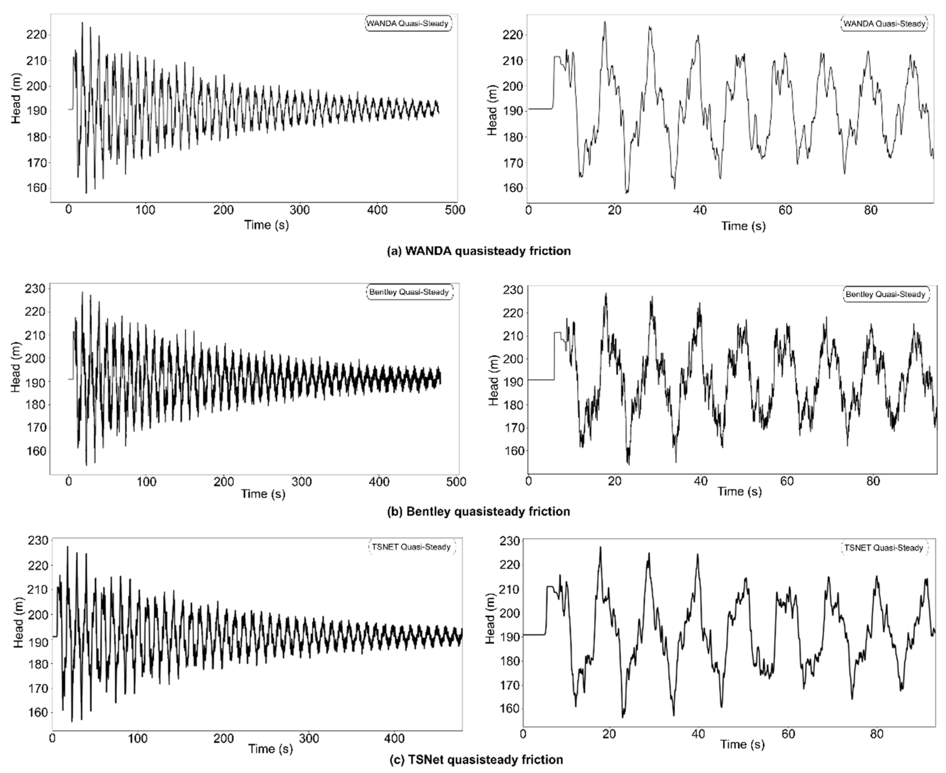
The quasisteady model simulations illustrated in Figure 6 revealed the different software attributes using the benchmark network in Figure 2. First of all, the wave shape and attenuation are similar for WANDA and Bentley Hammer. However, the wave shape of TSNet had the same waveshape until the fifth peak, and then the wave shape attributes started to be significantly different. Regarding the first peak amplitude, it was noticed that WANDA, TSNet, and Bentley had almost the same amplitude of 214.1, 215.8, and 217.5 m. During the whole simulation period, it was noticed that the overall damping of WANDA was slightly higher than TSNet; however, Bentley Hammer showed the least damping performance. Finally, it can be easily deduced from Figure 6 that WANDA provided the smoothest curves followed by TSNet then Hammer.
The difference in damping and wave shape was a matter of interest. The difference might be attributed to the hydraulics algorithm used for each software. WANDA and Bentley Hammer had a similar wave shape; hence, the hydraulic algorithms are relatively similar. Besides that, the wave speed adjustment scheme was different in TSNet from Hammer and WANDA. Therefore, it is essential to ensure the adapted wave celerity during the comparison. Regarding the discretization, it is also different in TSNet and the other software.
3.3.2. Vítkovský Friction Comparison
Vítkovský’s friction model is the only currently implemented friction model in commercial software. This is because it can be simply computed without intensive computational efforts, and it provides moderately high accuracy. Therefore, it was a matter of interest to compare the unsteady friction model in WANDA and the unsteady friction model in the competitive commercial software such as Bentley Hammer and TSNet using the same benchmark network demonstrated in Figure 2.
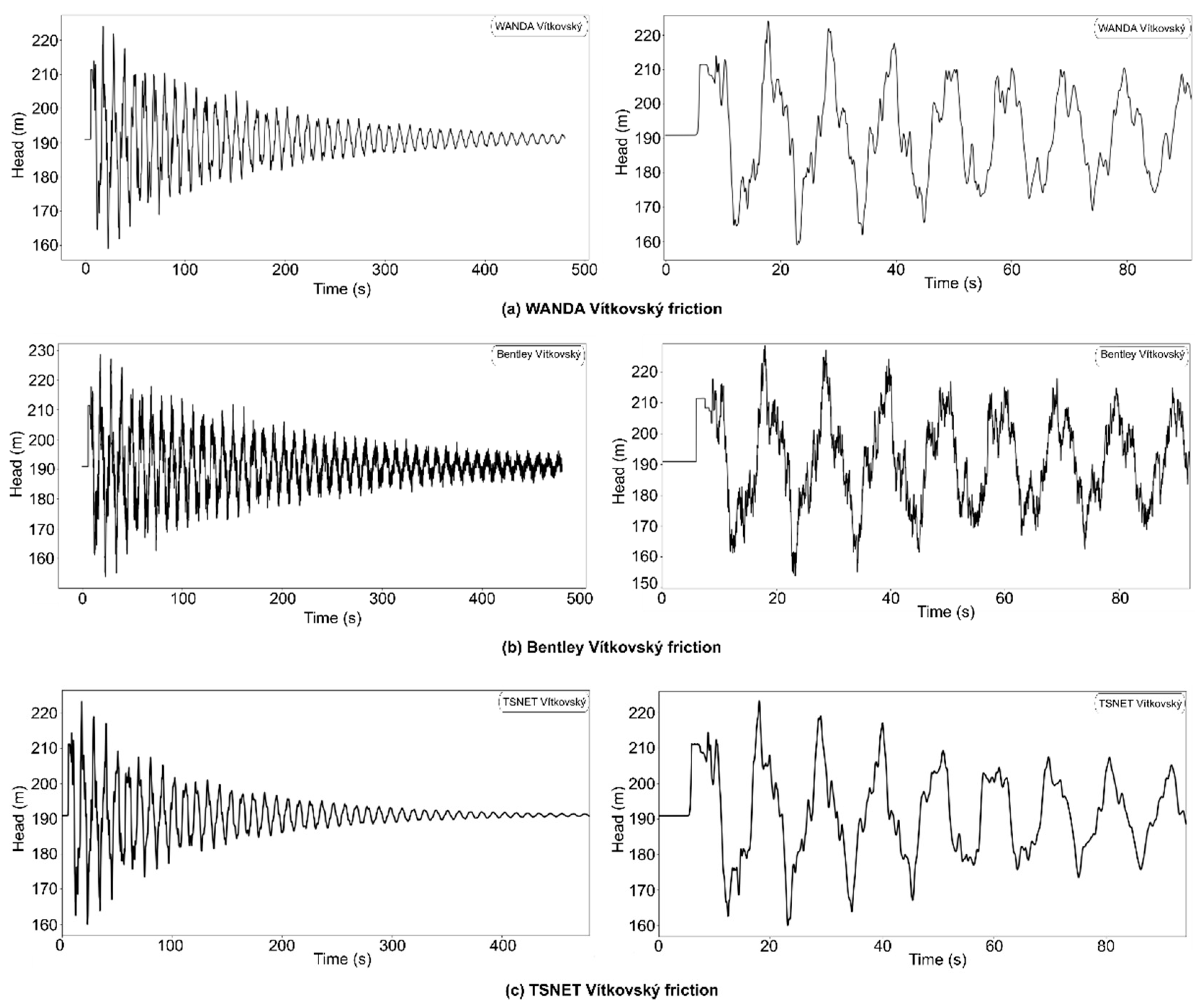
Figure 7 illustrates the different responses of the compared software. Similar to the quasisteady friction simulation, WANDA and Bentley’s wave shape and attenuation were similar while TSNet wave shape differs significantly after the fifth peak. The TSNet Vítkovský model provided the strongest damping followed by WANDA then Hammer. Regarding the simulation smoothness, WANDA and TSNet showed a similar smooth behavior followed by Hammer, which was the least smooth one.
4. Conclusions and Future Perspectives
The conventional (quasi) steady friction assumption used in standard engineering practice for water hammer analyses limits transient simulations as wave damping becomes quickly underestimated due to the effect of unsteady friction. The computation of unsteady friction in commercial software is therefore mandatory for the accurate simulation of hydraulic transients, especially for those engineering applications requiring more in-depth insight into the pressure history (e.g., pipe flaw detection). Different unsteady friction models have been studied and compared based on developed criteria that focus on required user inputs, stability, accuracy, and computational efforts. The most-suited unsteady friction model that fits the engineering practices in the tested commercial software (i.e., WANDA) was Vítkovský’s model. The model has been implemented in WANDA and verified with other commercial software and experimental data. The model has also been tested on different hydraulic urban networks, with varying materials of pipe. It was found that incorporating the unsteady friction improves the description of the wave damping compared to the conventionally used quasisteady friction model.
Hydraulic transient software such as WANDA are becoming usual tools for water distribution analyses; however, their performance requires further improvement. For instance, implementation of the pipe-wall rheological behavior in WANDA for pipe networks simulation is crucial, since PVC and HDPE pipes are introduced more often to water distribution networks. The WANDA upgraded version presented should be tested for a set of engineering applications, e.g., leakage detection by means of inverse transient analysis.
Author Contributions
Conceptualization, D.F.; Data curation, O.M.A. and S.v.d.Z.; Formal analysis, O.M.A.; Funding acquisition, M.K.; Investigation, O.M.A.; Methodology, D.F.; Project administration, D.F. and M.K.; Resources, D.F.; Software, O.M.A. and S.v.d.Z.; Supervision, D.F. and M.K.; Validation, O.M.A.; Visualization, D.F.; Writing—Original draft, O.M.A.; Writing—Review & Editing, D.F. and M.K. All authors have read and agreed to the published version of the manuscript.
Funding
The APC of this paper was funded by IHE Delft Institute for Water Education.
Institutional Review Board Statement
Not applicable.
Informed Consent Statement
Not applicable.
Data Availability Statement
The data presented in this study are available within the article. If extended data are required, additional data are available on request from the corresponding author.
Acknowledgments
The authors would like to express their gratitude to Silvia Meniconi from the University of Perugia for constructive comments and feedback. O.M. Abdeldayem thanks the Erasmus+ International Master of Science in Environmental Technology and Engineering (IMETE) for supporting the M.Sc program at UCT Prague (Czech Republic), IHE Delft (Netherlands), and Ghent University (Belgium). O.M.A. pays his sincerest thanks to Mostafa Saleh from IHE Delft of Water Education for the support and advice during the programming phase.
Conflicts of Interest
There are no conflict to declare.
References
- Bettaieb, N.; Taieb, E.H. Assessment of Failure Modes Caused by Water Hammer and Investigation of Convenient Control Measures. J. Pipeline Syst. Eng. Pract. 2020, 11, 04020006. [Google Scholar] [CrossRef]
- Kanakoudis, V.K. A troubleshooting manual for handling operational problems in water pipe networks. J. Water Supply Res. Technol. AQUA 2004, 53, 109–124. [Google Scholar] [CrossRef]
- Meniconi, S.; Cifrodelli, M.; Capponi, C.; Duan, H.F.; Brunone, B. Transient Response Analysis of Branched Pipe Systems toward a Reliable Skeletonization. J. Water Resour. Plan. Manag. 2021, 147, 04020109. [Google Scholar] [CrossRef]
- Chaudhry, M.H. Applied Hydraulic Transients; Springer: London, UK, 2013. [Google Scholar] [CrossRef]
- Huang, Y.; Zheng, F.; Duan, H.F.; Zhang, Q. Multi-Objective Optimal Design of Water Distribution Networks Accounting for Transient Impacts. Water Resour. Manag. 2020, 34, 1517–1534. [Google Scholar] [CrossRef]
- Kerger, F.; Erpicum, S.; Dewals, B.J.; Archambeau, P.; Pirotton, M. 1D unified mathematical model for environmental flow applied to steady aerated mixed flows. Adv. Eng. Softw. 2011, 42, 660–670. [Google Scholar] [CrossRef] [Green Version]
- Ying, K.; Chu, J.; Qu, J.; Luo, Y. A model and topological analysis procedures for a pipeline network of variable connectivity. Adv. Eng. Softw. 2012, 48, 40–51. [Google Scholar] [CrossRef]
- Quildoran, J.T. Water hammer analysis using an implicit finite-difference method. Ingeniare Rev. Chil. Ing. 2018, 26, 307–318. [Google Scholar]
- Selecting the Transient Friction Method. (Bentley Hammer). Available online: https://docs.bentley.com/LiveContent/web/Bentley%20WaterGEMS%20SS6-v1/en/GUID-ED359106-8917-491F-A42C-38CB1AD0C117.html (accessed on 11 February 2021).
- Xing, L.; Sela, L. An overview of the transient simulation in water distribution networks (TSNet). In Proceedings of the World Environmental and Water Resources Congress 2020: Hydraulics, Waterways, and Water Distribution Systems Analysis, Henderson, NV, USA, 17–21 May 2020; pp. 282–289. [Google Scholar]
- Cao, H.; Nistor, I.; Mohareb, M. Effect of boundary on water hammer wave attenuation and shape. J. Hydraul. Eng. 2020, 146, 04020001. [Google Scholar] [CrossRef]
- Ferràs, D.; Manso, P.A.; Schleiss, A.J.; Covas, D.I. One-dimensional fluid–structure interaction models in pressurized fluid-filled pipes: A review. Appl. Sci. 2018, 8, 1844. [Google Scholar] [CrossRef] [Green Version]
- Mandair, S.; Magnan, R.; Morissette, J.F.; Karney, B. Energy-Based Evaluation of 1D Unsteady Friction Models for Classic Laminar Water Hammer with Comparison to CFD. J. Hydraul. Eng. 2020, 146, 04019072. [Google Scholar] [CrossRef]
- Duan, H.F.; Meniconi, S.; Lee, P.J.; Brunone, B.; Ghidaoui, M.S. Local and integral energy-based evaluation for the unsteady friction relevance in transient pipe flows. J. Hydraul. Eng. 2017, 143, 04017015. [Google Scholar] [CrossRef] [Green Version]
- Martins, N.M.C.; Brunone, B.; Meniconi, S.; Ramos, H.M.; Covas, D.I.C. CFD and 1D approaches for the unsteady friction analysis of low Reynolds number turbulent flows. J. Hydraul. Eng. 2017, 143, 04017050. [Google Scholar] [CrossRef]
- Covas, D.; Stoianov, I.; Ramos, H.; Graham, N.; Maksimović, Č.; Butler, D. Water hammer in pressurized polyethylene pipes: Conceptual model and experimental analysis. Urban Water J. 2004, 1, 177–197. [Google Scholar] [CrossRef]
- Bergant, A.; Tijsseling, A.S.; Vítkovský, J.P.; Covas, D.I.; Simpson, A.R.; Lambert, M.F. Parameters affecting water-hammer wave attenuation, shape and timing—Part 1: Mathematical tools. J. Hydraul. Res. 2008, 46, 373–381. [Google Scholar] [CrossRef] [Green Version]
- Ferràs, D.; Manso, P.A.; Schleiss, A.J.; Covas, D.I. Fluid-structure interaction in straight pipelines: Friction coupling mechanisms. Comput. Struct. 2016, 175, 74–90. [Google Scholar] [CrossRef]
- Ferràs, D.; Manso, P.A.; Covas, D.I.C.; Schleiss, A.J. Fluid–structure interaction in pipe coils during hydraulic transients. J. Hydraul. Res. 2017, 55, 491–505. [Google Scholar] [CrossRef]
- Shamloo, H.; Norooz, R.; Mousavifard, M. A review of one-dimensional unsteady friction models for transient pipe flow. Cumhur. Üniv. Fen-Edeb. Fak. Fen Bilim. Derg. 2015, 36, 2278–2288. [Google Scholar]
- Bergant, A.; Ross Simpson, A.; Vìtkovsky, J. Developments in unsteady pipe flow friction modelling. J. Hydraul. Res. 2001, 39, 249–257. [Google Scholar] [CrossRef] [Green Version]
- Jensen, R.; Kær Larsen, J.; Lindgren Lassen, K.; Mandø, M.; Andreasen, A. Implementation and validation of a free open source 1d water hammer code. Fluids 2018, 3, 64. [Google Scholar] [CrossRef] [Green Version]
- Soares, A.K.; Martins, N.; Covas, D.I. Investigation of transient vaporous cavitation: Experimental and numerical analyses. Procedia Eng. 2015, 119, 235–242. [Google Scholar] [CrossRef] [Green Version]
- Hino, M.; Sawamoto, M.; Takasu, S. Study on the transition to turbulence and frictional coefficient in an oscillatory pipe flow. Trans. JSCE 1977, 9, 282–284. [Google Scholar]
- Daily, J.W.; Hankey, W.L., Jr.; Olive, R.W.; Jordaan, J.M., Jr. Resistance Coefficients for Accelerated and Decelerated Flows through Smooth Tubes and Orifices; No. 55-SA-78; Massachusetts Institute of Technology: Cambridge, MA, USA, 1956. [Google Scholar]
- Brunone, B.; Golia, U.M.; Greco, M. Some remarks on the momentum equation for fast transients. In Proceedings of the International Meeting on Hydraulic Transients with Column Separation, Valencia, Spain, 4–6 September 1991; pp. 201–209. [Google Scholar]
- Vítkovský, J.P.; Lambert, M.F.; Simpson, A.R.; Bergant, A. Advances in unsteady friction modelling in transient pipe flow. In Proceedings of the 8th International Conference on Pressure Surges 2000, The Hague, The Netherlands, 12–14 April 2000; pp. 471–482. [Google Scholar]
- Vardy, A.E.; Brown, J.M.B. Transient turbulent friction in smooth pipe flows. J. Sound Vib. 2003, 259, 1011–1036. [Google Scholar] [CrossRef]
- Vardy, A.E.; Brown, J.M.B. Transient turbulent friction in fully rough pipe flows. J. Sound Vib. 2004, 270, 233–257. [Google Scholar] [CrossRef]
- Bergant, A.; Simpson, A.R.; Scotland, M. Estimating unsteady friction in transient cavitating pipe flow. In Proceedings of the 2nd International Conference on Water Pipeline Systems, Edinburgh, UK, 24–26 May 1994. [Google Scholar]
- Twyman, J. Water hammer analysis using a hybrid scheme. Rev. Ing. Obras Civ. 2017, 7, 16–25. [Google Scholar]
- Vítkovský, J.P.; Bergant, A.; Simpson, A.R.; Lambert, M.F. Systematic evaluation of one-dimensional unsteady friction models in simple pipelines. J. Hydraul. Eng. 2006, 132, 696–708. [Google Scholar] [CrossRef] [Green Version]
- Adamkowski, A.; Lewandowski, M. Experimental examination of unsteady friction models for transient pipe flow simulation. J. Fluids Eng. Trans. ASME 2006, 128, 1351–1363. [Google Scholar] [CrossRef]
- Carstens, M.R.; Roller, J.E. Boundary-shear stress in unsteady turbulent pipe flow. J. Hydraul. Div. 1959, 85, 67–81. [Google Scholar] [CrossRef]
- Shuy, E.B.; Apelt, C.J. Experimental studies of unsteady wall shear stress in turbulent flow in smooth round pipes. In Conference on Hydraulics in Civil Engineering 1987: Preprints of Papers, Proceedings of the Conference on Hydraulics in Civil Engineering 1987, Melbourne, Australia, 12–14 October 1987; Institution of Engineers: Barton, Australia, 1987; p. 137. [Google Scholar]
Figure 1.
Simple network structure.
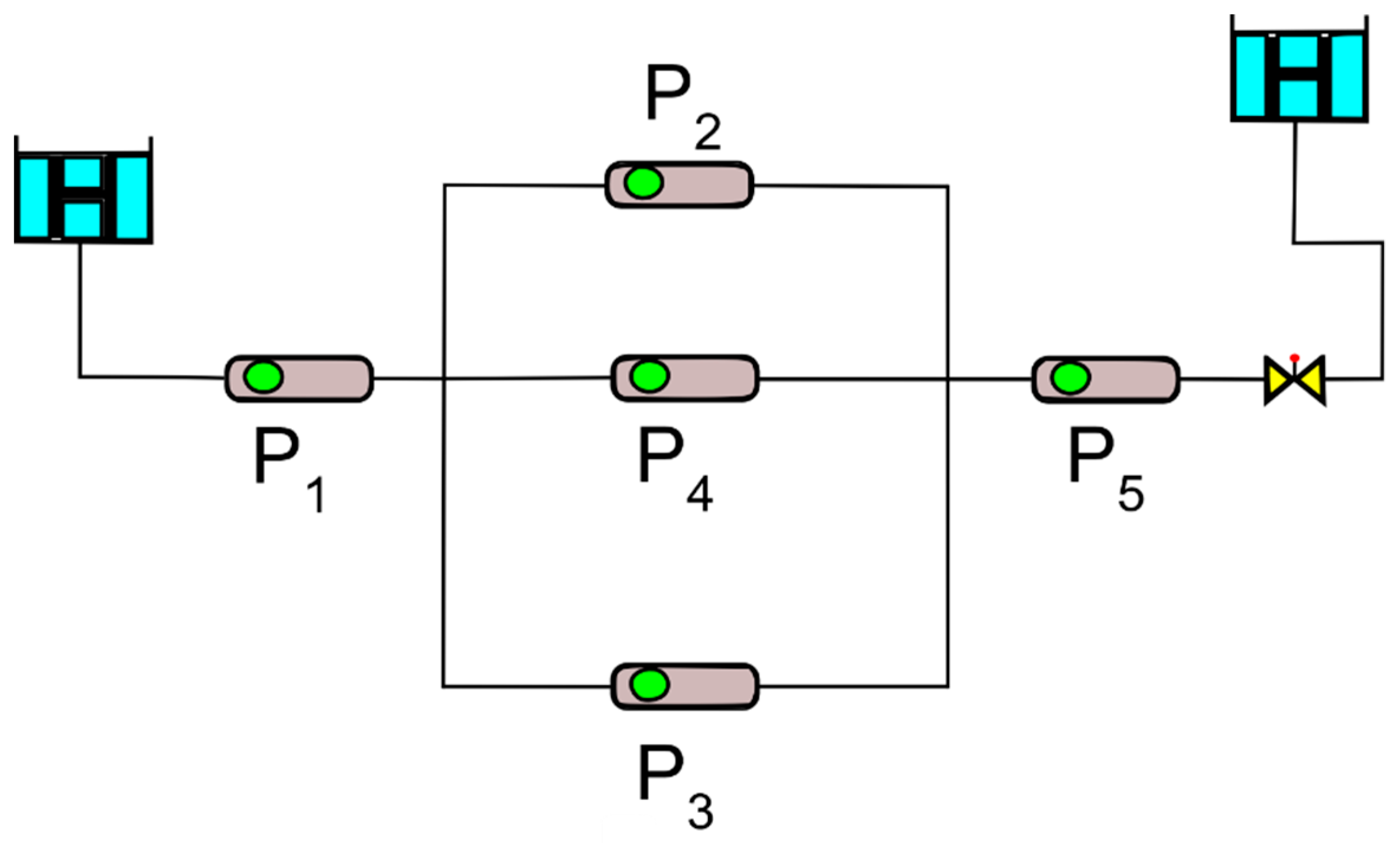
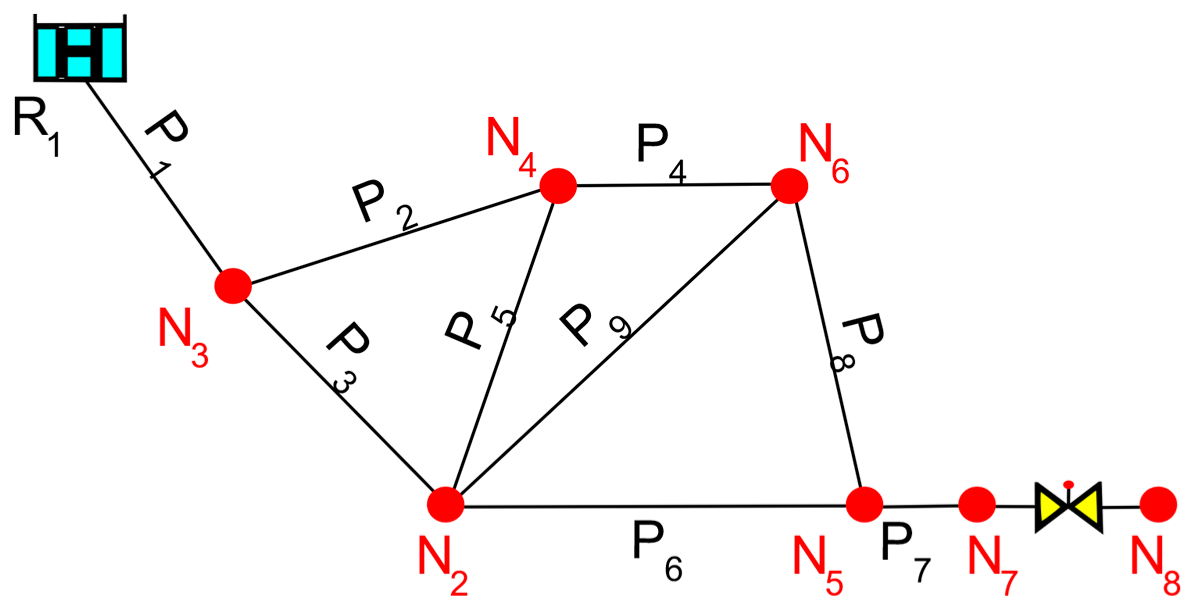
Figure 2.
Benchmark network structure.

Figure 3.
Simulation of different friction models.

Figure 4.
Vítkovský’s model in WANDA and Python.
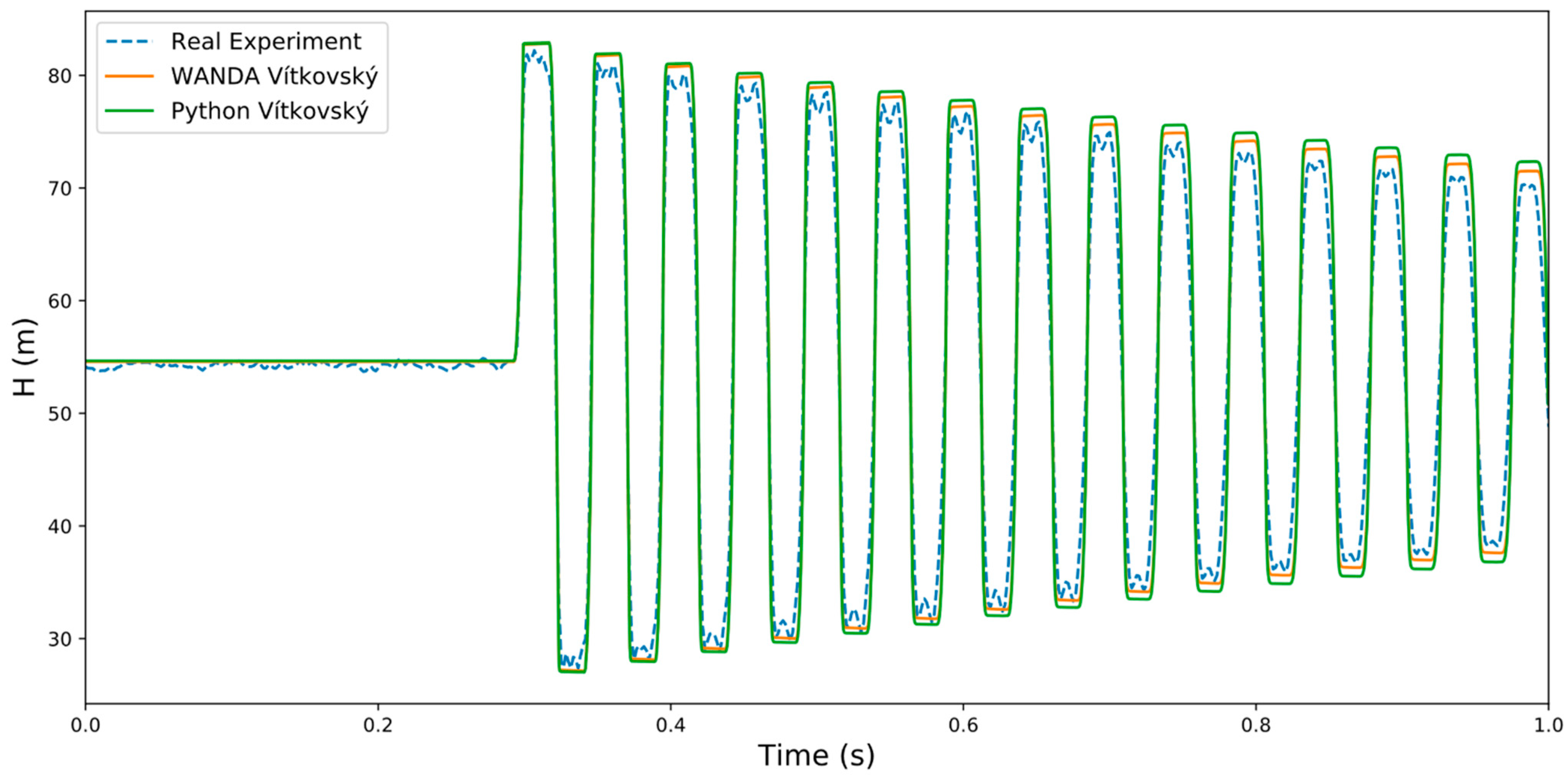
Figure 5.
Effect of pipe materials at simple networks. (a): Copper; (b): Steel; (c): Reinforced concrete; (d): Greycast iron; (e): PVC; (f): Mixture of pipes.
Figure 5.
Effect of pipe materials at simple networks. (a): Copper; (b): Steel; (c): Reinforced concrete; (d): Greycast iron; (e): PVC; (f): Mixture of pipes.
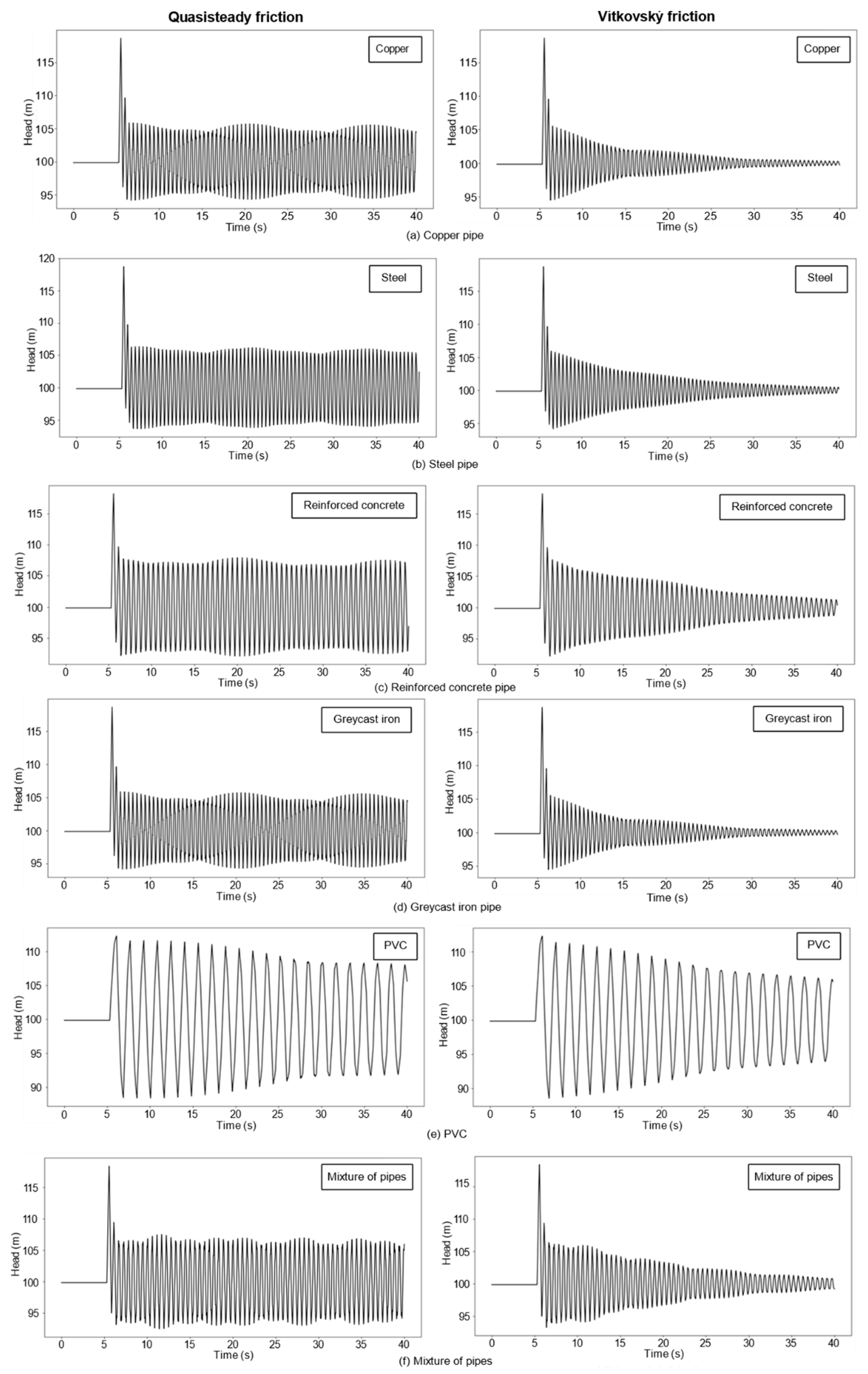
Figure 6.
Comparison of quasisteady friction in commercial software. (a): Wanda quasisteady friction; (b): Bentley quasisteady friction; (c): TSNet quasisteady friction.
Figure 6.
Comparison of quasisteady friction in commercial software. (a): Wanda quasisteady friction; (b): Bentley quasisteady friction; (c): TSNet quasisteady friction.

Figure 7.
Comparison of Vítkovský friction in commercial software. (a): Wanda Vítkovský friction; (b): Bentley Vítkovský friction; (c): TSNet Vítkovský friction.
Figure 7.
Comparison of Vítkovský friction in commercial software. (a): Wanda Vítkovský friction; (b): Bentley Vítkovský friction; (c): TSNet Vítkovský friction.


Table 1.
Available water hammer commercial software.
| Institution | Software Name | Solution Method | Friction Model |
|---|---|---|---|
| Applied Flow Technology | AFT Impulse | MoC | Quasisteady |
| Flow Science Inc. | FLOW 3-D | TruVOF | Steady |
| Hydromantis Inc. | ARTS | MoC | Steady |
| University of Auckland | HYTRAN | MoC | Vítkovský |
| BHR Group | FLOWMASTER 2 | MoC | Steady |
| Bentley Systems, Inc. | HAMMER | MoC | Vítkovský |
| Stoner Associates, Inc. | LIQT | MoC | Steady |
| DHI | HYPRESS | Finite-Difference Method | Steady |
| University of Cambridge | PIPENET | MoC | Steady |
| University of Kentucky | SURGE | Wave Method (WM) | Steady |
| University of Texas at Austin | TSNet | MoC | Vítkovský |
| University of Toronto | TRANSAM | MoC | Steady |
| University Politécnica de Valencia | DYAGATS | MoC | Steady |
| University Politécnica de Valencia | ALLIEVI | MoC | Steady |
| Deltares | WANDA | MoC | Quasisteady |
| US Army Corps Engineers | WHAMO | Finite-Difference Method | Steady |
| DHI | MIKE URBAN | MoC | Steady |
| Innovyze | H2O SURGE | WM | Steady |
| KYPIPE | SURGE | WM | Steady |
| EPA | EPA SURGE | WM | Steady |
| Unisont Engineering, Inc. | uSLAM | MoC | Steady |
Table 2.
Unsteady friction models’ categories and equations.
| Friction Model Category | Model Name | Equation | Equation Number | Reference |
|---|---|---|---|---|
| Steady and quasisteady friction | Darcy Weisbach | (5) | [4] | |
| Instantaneous mean flow velocity | Hino | (6) | [24] | |
| Instantaneous mean flow velocity and local acceleration | Daily | (7) | [25] | |
| Instantaneous mean flow velocity, local acceleration, and convective acceleration | Brunone | (8) | [26] | |
| Instantaneous mean flow velocity, local acceleration, and convective acceleration | Vítkovský | (9) | [27] | |
| Instantaneous mean flow velocity and past velocity changes weights | Convolutional model | (10) | [28,29] | |
| Vardy and Brown weighting function | (11) |
Where, f is Darcy’s friction factor, L is the length of pipe (m), g is the acceleration due to gravity (m/s2), D is the inner diameter of the pipe (m), V (m/s) is the mean flow velocity, v (m2/s) is the viscosity, c2 is an empirical constant, a (m/s) is the wave celerity, k is Brunone’s friction coefficient, and the sign term provides the right sign for the convection term for all potential flows, acceleration, or deceleration phases.
Table 3.
Simple synthetic network characteristics.
| Component | Specification | |
|---|---|---|
| Elevated tank | Head (m) | 100 |
| Final tank | Head (m) | 0 |
| P1, P5 | Length (m) | 100 |
| Diameter (mm) | 200 | |
| Elevation (m) | 0 | |
| P2, P3, P4 | Length (m) | 50 |
| Diameter (mm) | 100 | |
| Elevation (m) | 0 |
Table 4.
Young modulus properties of pipes.
| Pipe Material | Young Modulus (N/m2) |
|---|---|
| Copper | 1.17 × 10¹¹ |
| Steel | 2.04 × 10¹¹ |
| Reinforced concrete | 4.50 × 10¹⁰ |
| Gray cast iron | 1.30 × 10¹¹ |
| Polyvinyl chloride (PVC) | 3.00 × 10⁹ |
Table 5.
Properties of the benchmark network.
| D | Length (m) | Wave Celerity (m/s) | Diameter (mm) | Roughness (mm) |
|---|---|---|---|---|
| VALVE-A | - | - | 184 | |
| P1 | 610 | 1271 | 900 | 0.26 |
| P2 | 910 | 1269 | 750 | 2.5 |
| P3 | 610 | 1271 | 600 | 0.8 |
| P4 | 457 | 1269 | 450 | 2.5 |
| P5 | 549 | 1220 | 450 | 0.4 |
| P6 | 671 | 1243 | 750 | 0.27 |
| P7 | 1000 | 1282 | 900 | 0.30 |
| P8 | 457 | 1269 | 600 | 0.26 |
| P9 | 488 | 1251 | 450 | 0.6 |
Table 6.
Big O notation for different friction models.
| Friction Model | Big O (Algorithm) | R2 (Algorithm) | Big O (Friction Model) | R2 (Friction) |
|---|---|---|---|---|
| Steady friction | O(N) | 0.9995 | O(1) | 1 |
| Quasi-first-order | O(N) | 0.9998 | O(N) | 0.9995 |
| Quasi-second-order | O(N) | 0.9998 | O(N) | 0.9994 |
| Hino | O(N) | 0.9984 | O(N) | 0.9991 |
| Daily | O(N) | 1 | O(N) | 0.9996 |
| Brunone | O(N) | 0.9969 | O(N) | 0.9998 |
| Vítkovský | O(N) | 0.9970 | O(N) | 0.9999 |
| Vardy and Brown | O(N2) | 1 | O(N2) | 0.9999 |
Table 7.
Weighted average comparison between friction models.
| Full Score | Weight | Steady Friction | Quasi 1st Order | Quasi 2nd Order | Hino | Daily | Brunone | Vítkovský | Vardy and Brown | |
|---|---|---|---|---|---|---|---|---|---|---|
| User input | 10 | 1 | 10 | 10 | 10 | 10 | 7 | 10 | 10 | 10 |
| Computational efforts | 10 | 3 | 10 | 9.5 | 9 | 9 | 9 | 8 | 8 | 2 |
| Stability | 10 | 1 | 10 | 10 | 10 | 10 | 4 | 10 | 10 | 10 |
| Accuracy | 10 | 3 | 3 | 4 | 3 | 5 | 5 | 8 | 8.5 | 10 |
| Total | 80 | 8 | 59 | 60.5 | 59 | 62 | 53 | 68 | 69.5 | 56 |
Publisher’s Note: MDPI stays neutral with regard to jurisdictional claims in published maps and institutional affiliations. |
© 2021 by the authors. Licensee MDPI, Basel, Switzerland. This article is an open access article distributed under the terms and conditions of the Creative Commons Attribution (CC BY) license (http://creativecommons.org/licenses/by/4.0/).
Share and Cite
MDPI and ACS Style
Abdeldayem, O.M.; Ferràs, D.; van der Zwan, S.; Kennedy, M. Analysis of Unsteady Friction Models Used in Engineering Software for Water Hammer Analysis: Implementation Case in WANDA. Water 2021, 13, 495. https://doi.org/10.3390/w13040495
AMA Style
Abdeldayem OM, Ferràs D, van der Zwan S, Kennedy M. Analysis of Unsteady Friction Models Used in Engineering Software for Water Hammer Analysis: Implementation Case in WANDA. Water. 2021; 13(4):495. https://doi.org/10.3390/w13040495
Chicago/Turabian StyleAbdeldayem, Omar M., David Ferràs, Sam van der Zwan, and Maria Kennedy. 2021. "Analysis of Unsteady Friction Models Used in Engineering Software for Water Hammer Analysis: Implementation Case in WANDA" Water 13, no. 4: 495. https://doi.org/10.3390/w13040495
Note that from the first issue of 2016, this journal uses article numbers instead of page numbers. See further details here.