Methodology for Determining the Maximum Potentially Recoverable Energy in Water Distribution Networks

Abstract

The excess pressure available in water distribution networks (WDNs) is a relevant aspect in the management and appropriate handling of water resources. If a WDN meets the minimum performance criteria (minimum pressure and maximum flow), excess pressure can occur throughout the day, which is usually lost. These excesses could be considered as potentially recoverable energy (PRE). One way of taking advantage of this energy is to find the nodes on the network where this excess pressure is evident and try to analyze the possible amount of PRE. This work presents a methodology to determine the maximum PRE in a WDN. This methodology includes the locations of the points where the installation of recovery devices leads to this maximum PRE. The method is based on reducing pressures but maintaining circulating points through the lines. Additionally, a new energy balance that allows visualizing and breaking down in more detail all the energy found in a WDN is proposed. The analysis is carried out in an extended period considering different feeding points either by gravity or pumping. Finally, a network resilience index called the Potentially Recoverable Energy Index (PREI) in WDNs is proposed, with which it is possible to diagnose and determine how much energy could be recovered from the network. Study cases presented demonstrate the effectiveness of the methodology and will allow the development of optimizations in the operation of WDNs in favor of the good management of water and energy resources.

1. Introduction

Global demand for water has increased at a rate of 1% per year due to population growth, economic development and changes in consumption patterns, among other factors. This growth will continue for the next two decades. Industrial and domestic demand for water will increase faster than agricultural demand, although the agricultural sector will continue to be the largest consumer of water in the world. As the population in large cities increases, so does the consumption of water. This effect is even greater in countries with emerging or developing economies [1].

Usually, water distribution networks (WDNs) are designed for a maximum operating condition, guaranteeing in all cases certain operating conditions (maximum flow and minimum pressure). However, these operating conditions have a very low frequency of occurrence. Therefore, it is possible that much of the time excess pressure is supplied to the network. In addition to this excess energy supplied, there are other energy losses inherent to the network (friction losses, losses in passive elements and control devices, etc.). Consequently, under non-critical scenarios, the excess energy could be recovered with the appropriate devices. It is what could be called potentially recoverable energy (PRE) of a WDN.

Some studies carried out on PRE are mainly based on the energy diagnosis of the network [2]. This work allows end-uses to be determined with sufficient precision to identify the greatest inefficiencies (e.g., leaks, friction, pumps) and the greatest potential savings. Once the overall analysis is complete, the focus shifts to those aspects or solutions with the highest cost-benefit relationship. Other authors [3,4,5] propose pumps working as turbines (PATs) or performing control with pressure reducing valves (PRVs). Both cases seek to control excess pressure and its direct relationship with leaks in WDNs. The difference is the first would have PRE and the other would be associated with pressure control in the technical management of the networks. Samora et al. [6], study the PRE and propose a methodology to quantify the hydroelectric potential from excess energy in a network. Their results demonstrate the existence of PRE, but only for a single study case. Their methodology does not locate the best points to extract this energy, but rather performs an energy recovery (ER) on certain devices already installed. Likewise, they consider a premise there is no variation in the demands of the analyzed network.

In the search to take advantage of the energy lost in WDNs, different studies seek first to determine the base elements that will determine how much energy could be recovered. Specifically, these works identify the hydraulic parameters that have the greatest impact on energy performance in WDNs. In this sense, Hashemi et al. [7] propose to a methodology based on three steps: (i) determine the hydraulic parameters with the greatest influence on the energy performance of the WDN; (ii) carry out combinations of hydraulic parameters that allow distinguishing the most/least efficient pipelines from the energy point of view; and (iii) look for the effect that a pipeline rehabilitation (based on age or breakage rate) would have on the energy efficiency of WDNs. These actions are related by measuring the energy that can be recovered, and it is measured from the characteristics of the network. This is obtained by analyzing the relationship between the pipeline and hydraulic parameters such as the transported flow, roughness coefficient, pipeline diameter, unit losses, pressure, elevation and the hydraulic proximity to the main components of the WDN. In general, energy dynamics together with risk assessment, pipeline age, breakage rates and water quality can help prioritize pipeline replacement and rehabilitation, and should be considered as part of the big picture to improve the overall performance of a WDN [7]. These correlations allow to initially identify the parameters that could be relevant for the installation of possible ER points or devices. In other words, it is a study more focused on the individual analysis of the pipelines than on the joint effect that all of them have.

One of the most studied elements in energy recovery is the replacement of PRV by turbines, microturbines or PATs in WDNs. According to Pérez-Sánchez et al. [8], the use of PATs have positive aspects, since they can replace PRVs to dissipate excess flow energy, obtaining adequate efficiency values. Other advantages of using PATS are lower investment costs and the existence of a high number of commercial machines available. However, it is important to consider the main negative aspects of PATs, such as their low efficiency when they operate outside their best efficiency point (BEP). Sinagra et al. [9] propose the replacement of PRVs with cross-flow turbines with positive outlet pressure since these generate the same energy dissipation as PRVs but allowing hydroelectric generation. The regulation of these turbines requires a coupling between hydraulics and electronics to improve the efficiency of hydroelectric generation [10]. This hydroelectric use can be significant as these devices provide high efficiencies and low construction costs. At the same time, they have the ability to control the pressure and discharge flow while generating electrical power.

Other ER devices are the Green Valves proposed by Ferrarese and Malavasi [11]. These are devices that replace traditional PRVs. They have the ability to recover energy and at the same time allow real-time control of pressures and flows in the network. They can be a tool that facilitates optimization and the network management.

The ER in a WDN can be approached from two points of view. The first one considers a global approximation of the problem, considering at the same time the different sources of energy (pumps, solar panels, wind turbines, storage batteries) [12]. This type of analysis seeks to combine the energy required in the network, taking into account both the residential loads and the water storage capacity in the tanks, with the energy production capacity. At this point the installation of ER devices takes a completely different approach. The second is focused on a local perspective in which only the actions that are performed directly on the WDN are analyzed. This line includes works such as those of Ramos et al. [13], García et al. [14] and Rosado et al. [15].

Ramos et al. [13] carry out an experimental study of an Inline Pumped Storage Hydropower (IPSH). It is a system that incorporates a turbine and an auxiliary tank as an ER device in a conventional pumping system. Its numerical model allows an evaluation of the IPSH solution, obtaining significant contributions both at the ER level and the design level of the devices involved. Among other studies in this field, Rosado et al. [15] determine the minimum parameters of the equipment studied in which the pump could work as a turbine without generating major implications in the operation of the equipment. Additionally, García et al. [14] evaluate not only the replacement of PRVs by PATs generating ER, but also the influence of this replacement in the reduction of the pressure driven consumption and the leakage reduction associated with the pressure control in the network. Along this same line, Monteiro et al. [16] develop a methodology for calculating the head and flow conditions required in micro hydroelectric plants for energy recovery, which take advantage of the excess pressure in WDNs.

Although the advantages and disadvantages of using PATs as ER devices are understood, it is important to define very well the location of these elements to be used in the most efficient way. There are some previous papers that work on ER in WDNs. In these cases, the best location of micro hydroelectric plants is sought to recover the maximum energy. The work of Telci [17] develops a methodology for the location of these plants and compares its application to pump and gravity driven networks. Telci and Aral [18] develop a methodology that determines this excess energy using intelligent management in the operation of the network and analyzing the best placement of microturbines in the system. In this way, the best microturbine locations and their operation program allow the recovery of the greatest amount of energy available, satisfying at the same time the current demand for water supply and the minimum pressures required. Their results show the location and type of microturbine have significant effects on optimal operating schemes. Definitely, the potential excess energy available from a WDN can vary significantly depending on the complexity and type of supply (pumping or gravity) of the network.

Similarly, Chacon et al. [19] develop a methodology to select the best PATs with the lowest payback period applied to irrigation networks. Other studies focus on particular cases or experimental prototypes on a laboratory scale [20,21]. Some authors such as Merielles et al. [22] even consider ER as part of the pipeline design process in a WDN. There are also studies on ER from hot wastewater in buildings [23], although this is beyond the control of the WDN managers. In short, until now there are methodologies or models that allow determining the ER in WDN that are specific for particular cases and that seek the final selection of a PAT. However, no previous work considers the effects that the network topology or a precise location of the possible recovery devices can have on the recovered energy.

In addition, previous studies focus on the energy that can be recovered in the network, but it is not specified if there is any type of energy that is recoverable by the user or other elements already installed. The only previous work that considers the network topology for the evaluation of the maximum PRE is the one developed by Iglesias-Castelló et al. [24]. However, the proposed balance was not specifically geared towards energy recovery. In other words, an ER is considered, but the possibility that the network already had ER devices already installed was not considered.

Any excess pressure over the minimum required is excess energy delivered. Part of this energy can be recovered in the network by installing different ER devices. However, the topology of the network means that to maintain the minimum pressure in some nodes it is necessary to have pressures higher than the minimum in others. At these nodes, the excess energy supplied cannot be recovered in the network. However, users connected to these nodes could install small ER devices to harness that energy. It is what in this work is called the PRE by users. Thus, the main objective of this work is to develop a new methodology that allows knowing the maximum PRE of a WDN, knowing the location of the ER devices required to reach said maximum, and discriminating between the PRE that can be recovered in the network from which only users can retrieve.

For this, the work addresses three main stages. In the first one, a proposal is made for a new energy balance of a WDN considering both the PRE and the energy that is effectively recovered in the network by means of the elements already installed.

The second stage is the development of the methodology, which is based on a topological analysis of the network and on the assumption that the flow rates before and after installing the ER devices are the same. It is about extracting the most power from the WDN without affecting its performance. To avoid altering the operation of the network and to extract the maximum possible energy, it is considered a restriction to keep the flow rates of circulation through the lines fixed. The methodology requires the availability of the mathematical model of the WDN, since the results depend entirely on the reliability of the model. This model can be made with any hydro-informatics technique (GIS, SCADA, etc.). The important thing is the model accurately reflects the real behavior of the network. In this case, the EPANET [25] model has been used as a network behavior analysis tool.

The third stage is a consequence of the energy balance and the determination of the different components of the PRE. It is a proposal for a new resilience index for a WDN, the Potentially Recoverable Energy Index (PREI). The validation of this new resilience index, as well as the proposed methodology, is carried out through the study of four case studies. The comparative analysis of these cases allows to understand the applicability of the methodology and the significance of this resilience index.

2. Materials and Methods

The development of the main objective, to develop a methodology that determines the maximum PRE in a WDN, has been structured in three defined stages. In the first one, a new proposal for the energy balance of a WDN has been developed, explicitly considering both the PRE and the energy effectively recovered by means of RE devices such as turbines or PATs. The second stage consisted in defining the method that allows obtaining the maximum PRE based on assuming the flow distribution before and after the ER is the same. The third stage uses the results of both the energy balance and the PRE calculation to define a new resilience indicator for WDNs. This indicator focuses on the ER capacity of a network. The following sections analyze each of these three stages.

2.1. Energy Balance of a WDN

The energy analysis of a WDN must analyze all the energy used to transport water from the origin point to the final consumer. Some previous studies focus the idea of this analysis on the approach of the energy balance in a WDN [26], at the level of an analysis or state of the network [27] or as a potentially recoverable energy index [28]. Iglesias-Castelló et al. [24] propose a new energy balance. The proposal considers an energy supplied and energy consumed within the network. However, this balance does not specifically define the recovered energy that is recovered in the network. This suggests the need to expand the energy balance developed by Iglesias-Castelló et al. [24] to include a specific definition of recovered energy. 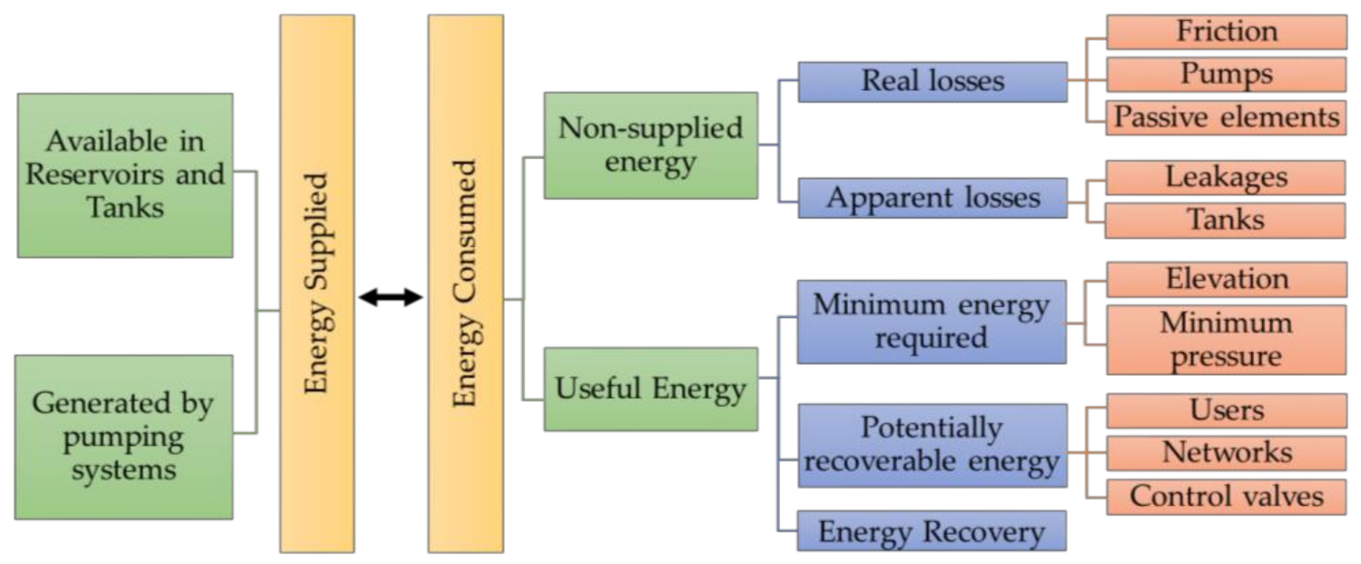Figure 1 presents the new proposed energy balance.

The proposed energy balance is based on the hypothesis of considering all the elements of the network (pipes, valves, pumps, accessories, etc.) as a system. At this point, the pressure nodes (reservoirs or tanks) are entry or exit points and therefore external to the system. Likewise, the consumption nodes are also exit points of the system. In other words, the system does not have any energy storage capacity and therefore the energy supplied will be equal to the energy dissipated inside the system plus the output energy that leaves the system through the nodes. The input energy to the system is what in the balance will be called energy supplied (E_sup). The sum of the dissipated energy and the output energy of the system is what will be called energy consumed (E_con). Logically, both energies (supplied and consumed) must be equal in the considered system.

The energy supplied to the network comes from two main sources: the potential energy stored in reservoirs and tanks that supply water to the system (E_e) and the electromechanical energy supplied by pumping systems (E_p). The potential energy E_e can be considered divided into two parts. The first one comes from the reservoirs in which the levels remain practically constant (E_e,r). The second one come from the tanks whose level varies during the operation of the network (E_e,t).

Now, the energy consumed can be broken down into two main terms, the non-supplied energy (E_nr) and the useful energy (E_u). Non-supplied energy includes all elements of the network where there is an unwanted loss of energy. This can be divided into two main components: real dissipated losses (E_d,r) and apparent losses (E_d,a). The real dissipated losses correspond to all the elements installed in the network that generate unavoidable energy dissipation, since they are intrinsically associated with their existence. These are: friction losses in the lines (E_d,f), losses in pumping systems (E_d,p) due to their inefficiency and losses in passive elements of the network (E_d,v) such as isolation valves, fittings, filters, etc. The valves that are part of this term (real losses, passive elements) do not fulfill a control function. That is, they are valves that function as passive elements in the WDN. There are other valves to perform control functions and installed to introduce controlled energy losses. These losses are intended to reduce pressure, limit flow or simply control the movement of water in the network. These types of valves are not passive elements since they have been installed with the idea that the introducing losses with certain objective.

On the other hand, there are other losses associated with non-supplied energy: the apparent dissipated losses. These correspond to the energy that has not been finally delivered to the users, but it cannot be considered as energy dissipation. The components of these losses are losses in leakage (E_d,l) and energy losses due to accumulation of water in tanks (E_d,t).

The other part of the energy consumed can be considered as useful energy. This useful energy would correspond to the sum of the minimum energy required in the nodes (E_min) and the excess of energy supplied with respect to the minimum required (E_ex). The minimum energy required (E_min) can be expressed as the sum of the topographic energy available (E_u,e) and the minimum pressure energy required at the nodes (E_u,p). The potentially recoverable energy represents the excess energy over the minimum supplied to the nodes. For its part, the energy recovered corresponds to that recovered in the network by already existing elements.

The excess energy E_ex is the main object of study of this work. A part of this energy excess is found in the energy recovery elements already installed in the network (E_R). Another part of this excess is found in the regulation and control valves installed in the WDN that could be replaced by ER devices. The remaining energy is an excess of energy supplied at the nodes above the minimum required. A part of this term may be recovered by installing ER devices in the network, but the network topology will cause another part of said excess to remain in the nodes.

The total excess energy above the required minimum pressure could be recovered by network users (PRE_u), that is, users could install small ER devices that take advantage of the excess pressure in the nodes with respect to the minimum pressure required. However, if the topographic conditions of the WDN allow it, part of this energy could be recovered by the network through ER devices (microturbines, PAT’s), which can be installed in different locations of the network with the aim to reduce and take advantage of the excess energy that exists in the nodes. If these elements are already installed, this energy is then considered as recovered energy (E_R). The energy specifically associated with the installed valves would be called potential recoverable energy by valves (PRE_v). The rest of the available excess energy is considered as potential recoverable energy by network (PRE_n). In summary, the proposed energy balance can be mathematically expressed as follows:

$${\mathrm{E}}_{\sup }={\mathrm{E}}_{\mathrm{e}}+{\mathrm{E}}_{\mathrm{p}}={\mathrm{E}}_{\mathrm{e},\mathrm{r}}+{\mathrm{E}}_{\mathrm{e},\mathrm{t}}+{\mathrm{E}}_{\mathrm{p}}$$

(1)

$$\begin{array}{c}{\mathrm{E}}_{\mathrm{con}}={\mathrm{E}}_{\mathrm{nr}}+{\mathrm{E}}_{\mathrm{u}}\hfill \\ \to 〈\begin{array}{c} {\mathrm{E}}_{\mathrm{nr}}={\mathrm{E}}_{\mathrm{d},\mathrm{r}}+{\mathrm{E}}_{\mathrm{d},\mathrm{a}}\to 〈\begin{array}{c}{\mathrm{E}}_{\mathrm{d},\mathrm{r}}={\mathrm{E}}_{\mathrm{d},\mathrm{f}}+{\mathrm{E}}_{\mathrm{d},\mathrm{p}}+{\mathrm{E}}_{\mathrm{d},\mathrm{v}}\hfill \\ {\mathrm{E}}_{\mathrm{d},\mathrm{a}}={\mathrm{E}}_{\mathrm{d},\mathrm{l}}+{\mathrm{E}}_{\mathrm{d},\mathrm{t}}\hfill \end{array}\hfill \\ {\mathrm{E}}_{\mathrm{u}}={\mathrm{E}}_{\mathrm{u},\mathrm{e}}+{\mathrm{E}}_{\mathrm{u},\mathrm{p}}={\mathrm{E}}_{\min }+{\mathrm{E}}_{\mathrm{ex}}={\mathrm{E}}_{\min }+\mathrm{PRE}+{\mathrm{E}}_{\mathrm{R}}\to 〈\begin{array}{c}{\mathrm{E}}_{\min }={\mathrm{E}}_{\mathrm{u},\mathrm{e}}+{\mathrm{E}}_{\mathrm{u},\mathrm{p}}\\ {\mathrm{E}}_{\mathrm{ex}}=\mathrm{PRE}+{\mathrm{E}}_{\mathrm{R}}\\ \mathrm{PRE}={\mathrm{PRE}}_{\mathrm{u}}+{\mathrm{PRE}}_{\mathrm{n}}+{\mathrm{PRE}}_{\mathrm{v}}\end{array}\end{array}\hfill \end{array}$$

(2)

The methodology proposed in this paper allows the PRE to be broken down, determining which part of the PRE can be recovered by valves (PRE_v), which part can be recovered on the network by installing new ER devices (PRE_n) and which part can only be recovered by users (PRE_u).

2.2. Methodology

The methodology to determine the maximum PRE in a WDN is proposed as an analysis that can be carried out at each moment of the dynamic simulation of the mathematical model, that is, the calculation of the PRE and its discrimination in its different terms can be done instantly. In other words, the power that can be recovered in the network can be calculated at each instant. Only when the energy recovery capacity is analyzed at each moment can the different recoverable powers be integrated to obtain the PRE.

Ultimately, the proposed method is exposed for a time instant. However, the complete methodology involves analyzing as many steady states as hydraulics calculation intervals the model has. The total PRE will be obtained from the instantaneous powers integrating these over time.

The methodology to determine the maximum PRE_n of a WDN in a generic instant of time considers the fulfillment of two hypotheses. The first one considers the pressure at the demand nodes must always be equal to or greater than the minimum pressure required. In the case of having nodes where the minimum pressure is not reached, the first objective is to modify the network or its operation mode in order to guarantee the minimum pressures required. Therefore, in these circumstances it does not make sense to apply the methodology for determining the maximum PRE.

The second hypothesis considers the flow distribution must remain constant before and after the installation of the ER devices. In general, the WDNs have an optimized operating mode that implies having determined the start and stop levels of the pumps, the temporary patterns of operation of the pumps, the setpoints variation of the control valves, etc. This operating mode is adjusted to the variations in demand over time. The proposed method to obtain the maximum PRE_n assumes the restriction of not modifying the network operating scheme. That is, the network must continue operating in the same way before and after applying the ER. This requirement implies to maintain the flow rates in the network before and after the ER. Logically, this does not imply that the flow rates must remain constant throughout the dynamic simulation of the network. As previously indicated, the analysis is performed instantly for each of the different hydraulic time steps of the model. In each analysis the ER is sought, keeping the flow rates constant. However, the flow rates in the network can vary from one moment to another. The only thing that must be maintained is the flow rates are the same before and after applying the method.

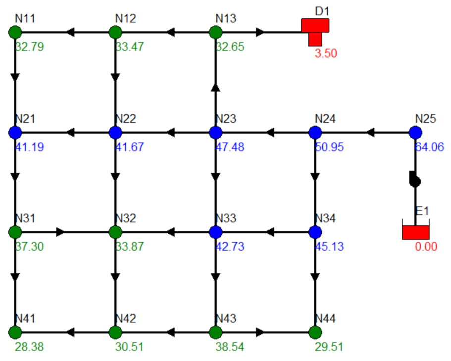
To illustrate the development of this methodology, the network represented in Figure 2 will be taken as an example, where the minimum pressure is set at 20 m. Data and details results of this network is collected in Supplementary Material. As it can be seen, this network presents an excess pressure regarding the minimum required in all demand nodes.

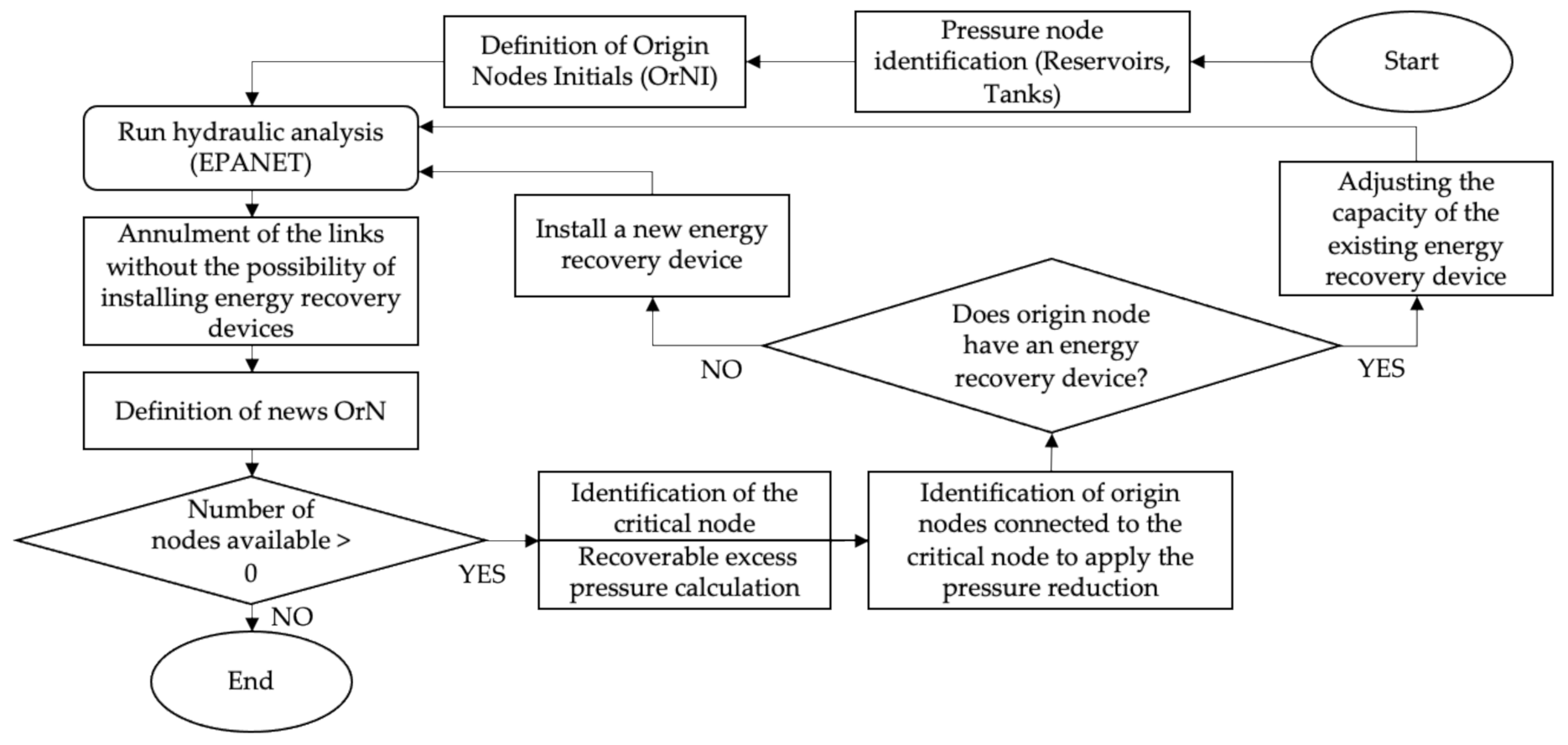
The first step of this methodology (see Figure 3) consists of defining the so-called Initial Origin Nodes (OrNI). These origin nodes are all those nodes of the network in which the pressure is fixed, whether they are tanks or reservoirs. From here, the hydraulic analysis of the network is carried out, which determines the directions of the flow in the lines.

After the hydraulic simulation, the first procedure consists of canceling the lines where there is no possibility of installing ER devices. If there is flow between reservoirs or tanks, this flow occurs through a series of pipelines in the network. The installation of any additional resistance in these lines would modify the flow. For this reason, it is not possible to install any ER unit in these lines.

In order to calculate these lines that must be canceled from the procedure, a topological scan of the network is carried out, starting from the OrNI that receive water until finding the OrNI that contribute water to the system. The objective of this topological scan is to determine the lines that connect the water flow from the water suppliers OrNIs to the water receiver OrNIs. The procedure begins by selecting a water receptor OrNI and the line connecting this OrNI with the network. Then, the upstream node of the line is determined. In the case of the network in the example in Figure 2, this node is N13. From this node, only the connected lines that provide water to the node are reviewed. The analysis of each of these lines is carried out using the same procedure: locate the upstream node and review the inlet pipes the node. This procedure is repeated recursively until one of the two search termination conditions occurs. There are two line review stop conditions, which suppose the completion of the topological scan. The first is to find a water supplier OrNI. The second is there are no more nodes and lines to be analyzed. The result of the process is a list of lines that interconnect the OrNIs following the direction of the water flow. In these lines it is not possible to add any ER device since this would mean the modification of the flow through the lines.

All lines in which the flow connects the OrNI are canceled. After finishing this procedure, it is necessary to carry out a new definition of the origin nodes (OrN). These OrN are those nodes connected at the same time to canceled and available lines. These new OrN go on to perform practically the same role as the initial OrNI and in them the head must be maintained, since otherwise the circulating flow through the lines would vary.

From this point, the process continues only if the OrN number is greater than zero. The stopping condition of the method is the absence of OrNs after the process of canceling lines in which it is not possible to install ER devices. Is the process continues, the Critical Node (CN) must be first identified. This CN is the demand node that presents the smallest pressure difference regarding the minimum pressure required. The difference between the CN pressure and the minimum required pressure is the excess pressure (ΔH_RE). This excess pressure is the loss that the ER devices located at the OrNs connected to the CN must introduce. In other words, in all the OrNs connected with the CN an ER device should be installed. The device must be installed on the line leading from the node in the direction of the CN location. If there are no ER devices on this line, a new element is created whose loss is ΔH_RE. In the case this line already has a device, it is not necessary to create a new device. In this case it is sufficient to add the ΔH_RE value to the loss already introduced by the ER device previously installed.

After this process, any other introduction of losses in the path that joins the CN with the OrNs would cause the CN to have a pressure lower than the minimum required. For this reason, the next stage of the process is to cancel the lines connecting the CN and the OrNs in the direction of flow circulation. The canceled lines generate the appearance of new OrNs. From this moment on, the existence of available nodes is analyzed again. In the event that there are no nodes available, the procedure is stopped. Otherwise the process is repeated, again identifying a new CN. This process is carried out iteratively until there is no node available within the network.

At the end of the procedure, the PRE for each ER device is obtained multiplying the circulating flow and the pressure loss that must be produced. At this point the identification of the PRE_n for the instant analyzed. In the case of having a dynamic model of the network, the following hydraulic time step should be analyzed. In this case, the process begins again with the hydraulic values of the network at this new moment. The process should be repeated as many times as there are hydraulic time steps.

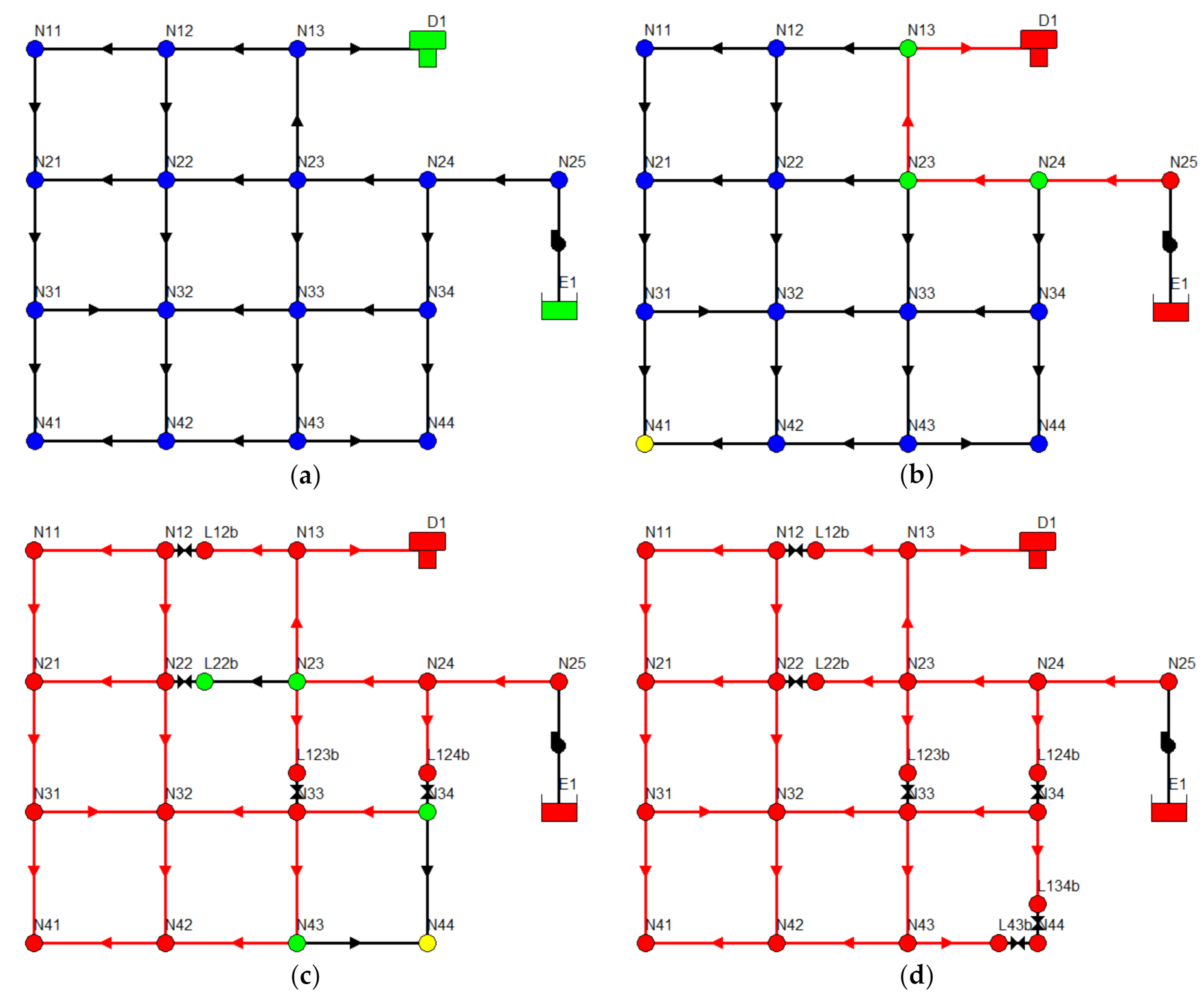
Next, the results of applying the methodology to the mathematical model of Figure 1 are presented. The example used is a steady-state model. Therefore, only one time step is analyzed and the process will not be repeated for different instants. The values to be obtained will be the powers that can be recovered at the instant represented by the model.

The data of this network is collected in the Supplementary Material section of this work. The initial iteration identifies two OrNIs: E1 and D1. Consequently, lines N13-D1, N23-N13, N24-N23, N25-N24 and E1-N25 are canceled, since the installation of an ER device in any of them implies a variation in flow distribution (see Figure 4, Initial iteration). Through this cancellation, new OrN are generated at nodes N13, N23 and N24, where the CN is N41 (pressure equal to 28.38 m), which implies an excess energy (pressure) of 8.38 m. This implies the installation of four ER devices on lines N12-N13, N22-N23, N23-N33 and N24-N34 (see Figure 4, Iteration 1). These new ERs lead to the cancellation of the lines marked in red (see Figure 4, Iteration 1) to keep the pressure at node N41 equal to 20 m. Therefore, new OrNs appear: NL22b, N23, N34 and N43.

In the next iteration, the CN corresponds to the N44, with an initial pressure of 29.51 m. Reducing the pressure to 20 m at this node implies incorporating two ER devices on lines N34-N44 and N43-N44, each with a pressure drop of 9.51 m. In summary, the final solution corresponds to that shown in Figure 4d. After the entry of the two ER devices of the last iteration, all the lines of the network are canceled, since it is not possible to install any ER device without modifying the flows. Therefore, the definitive process of the methodology is concluded.

The results of the different ER devices required in the network to obtain the maximum PRE are those shown in

Table 1. Energy recovery devices required in the example network.

No.	ID Link	ID ER	ER (kW)	% ER	% Accum. ER
1	Pipe L22	ER-22	1.28	38.65%	38.65%
2	Pipe L124	ER-124	0.71	21.44%	60.09%
3	Pipe L123	ER-123	0.65	19.60%	79.69%
4	Pipe L12	ER-12	0.61	18.56%	98.24%
5	Pipe L134	ER-134	0.05	1.52%	99.76%
6	Pipe L43	ER-43	0.01	0.24%	100.00%
			3.31	100%

. This table contains the results of the six ER devices that in Figure 4d are represented as valves in the network model. It should be noted that the analysis performed in this example is static (steady state analysis). For this reason, only potentially recoverable electrical powers are obtained.

Table 1 is ordered from highest to lowest ER capacity. In each ER device the line where its installed is collected. It should be noted that the details of these identifiers can be seen in the Supplementary Material of this work. The table also shows the power generated by each device, the percentage generated over the total and the accumulated percentage. The first four ER devices have quite a significant energy recovery capacity. The last two have a very insignificant contribution to the total. The total amount is 3.31 kW, which is the value of the PRE_n term. Once the PREn term has been calculated, the rest of the energy balance of the network can be completed (

Table 2. Energy analysis of the example network (kW).

Energy Balance				Example Network
Esup	Ee		Ee,r	2.86	2.86	39.48	39.48
			Ee,t	0.00
	Ep			36.62	36.62
Econ	Enr	Ed,r	Ed,f	10.17	10.17	14.29	39.48
			Ed,p	0.00
			Ed,v	0.00
		Ed,a	Ed,l	0.00	4.12
			Ed,t	4.12
	Eu	Emin	Eu,e	6.20	16.23	25.19
			Eu,p	10.03
		PRE	PREu	5.65	8.96
			PREn	3.31
			PREv	0.00
	ER			0.00	0.00

).

The energy balance of the network establishes that 37% of the power consumed (14.29 kW) is non-supplied power. The dissipated energy represents 71% (10.17 kW) of the non-supplied energy, while the rest (20%, 4.12 kW) are the apparent losses derived from the water delivered to tank D1. On the other hand, useful energy represents 63% (25.19 kW) of the total energy consumed. The minimum energy represents 41% of the energy consumed (16.23 kW) and represents slightly more than 64% of the useful energy. In this way, the PRE represents barely 23% (8.96 kW) of the energy consumed and close to 36% of the useful energy.

The calculation of the PRE_n in Table 1 allows us to discriminate the value of the PRE_u. The PRE that can only be recovered by network users, as it is not possible to recover in the network due to its own topology, represents 63% (5.65 kW) of the total PRE. In other words, only 37% (3.31 kW) of the PRE can be recovered in the network (PRE_n). This represents slightly more than 8% of all the energy consumed by the network.

In short, the ability to calculate the PREn allows us to know in some way the real excess energy of the network. It is therefore a measure of the oversizing of the network or of the capacity that this network may have to adapt to other operating conditions. That is why the next section addresses the use of this methodology as an indicator of resilience.

2.3. Resilience Index Based on ER

Another way to diagnose the hydraulic state of WDNs is through the resilience indexes that can be obtained in the study of each network. Resilience indexes in the WDN allow to visualize the capacity of the network in the event of failure events of the elements that compose it. Todini [29] defines a Resilience Index (RI) as the ratio between the excess energy in the nodes and the total energy excess supplied. In both cases, this excess energy is measured with respect to the minimum energy required in the nodes. Along the same line, Jarayam and Srinivasan [30] define a Modified Resilience Index (MRI) using the excess energy supplied at the consumption nodes as a percentage of the energy required. More recently, Paez and Filion [31] modify the MRI [30] in order to allow the comparison of the values between different WDN topologies by taking into account the pressure instead of the piezometric head in each node, obtaining the Centralized Modified Resilience Index (CMRI). In other words, the definition of these resilience indices is carried out based on an energy analysis of the operation of the network.

In the use of resilience as a design criterion for WDNs, Meirelles et al. [32] propose to rehabilitate trunk networks by considering the generation of electrical energy with the use of PATs, compensating the increase in resilience derived from the increase in pipeline diameters. During normal network operation, these devices would control pressure and produce electricity. In the event of an emergency, bypasses could be used to increase the pressure required in the network. The results obtained show that when using this combination (PATs and changing diameters), a small increase in trunk network diameters is enough to improve the resilience of the WDN.

The concept of PRE and its breakdown into PRE_u, PRE_n and PRE_v allow to define an index of energy efficiency of the network (I_ER). This index represents the capacity of the network to recover energy in the network, considering the relationship between the energy that can be recovered in the different elements of the network and the total energy consumed. Mathematically tis index could be defined as

$${\mathrm{I}}_{\mathrm{EE}}=1-\frac{{\mathrm{PRE}}_{\mathrm{n}}+{\mathrm{PRE}}_{\mathrm{v}}}{{\mathrm{E}}_{\mathrm{con}}}$$

(3)

Finally, the PRE quantification method allows defining a novel resilience index (PREI), which relates the ratio between the energy that can be recovered in the network elements (sum of PRE_n and PRE_v) and the excess energy supplied in the network. This energy excess is determined as the difference between the energy supplied (E_sum) and the minimum energy used. The minimum energy used is considered as sum of the minimum energy required (E_min), the real dissipated energy (E_d,r) and the energy stored in the tanks (E_d,t). To express the PREI mathematically, the energy consumed is defined from its relation to the energy supplied from the tanks (E_e), the energy supplied by the pumping stations (E_p):

$$\mathrm{PREI}=\frac{{\mathrm{PRE}}_{\mathrm{n}}+{\mathrm{PRE}}_{\mathrm{v}}}{{\mathrm{E}}_{\mathrm{e}}+{\mathrm{E}}_{\mathrm{p}}-{\mathrm{E}}_{\min }-{\mathrm{E}}_{\mathrm{d},\mathrm{t}}-{\mathrm{E}}_{\mathrm{d},\mathrm{r}}-{\mathrm{E}}_{\mathrm{R}}}$$

(4)

$${\mathrm{PRE}}_{\mathrm{v}}={\displaystyle \sum }_{\mathrm{v}=1}^{\mathrm{U}}{\displaystyle \sum }_{\mathrm{t}=0}^{{\mathrm{N}}_{\mathrm{inst}}}{\mathrm{Q}}_{\mathrm{v},\mathrm{t}}\times ∆{\mathrm{h}}_{\mathrm{v},\mathrm{t}}\times ∆{\mathrm{t}}_{\mathrm{t}}$$

(5)

$${\mathrm{E}}_{\mathrm{e}}={\displaystyle \sum }_{\mathrm{k}=1}^{\mathrm{R}}{\displaystyle \sum }_{\mathrm{t}=0}^{{\mathrm{N}}_{\mathrm{inst}}}{\mathrm{D}}_{{\mathrm{out}}_{\mathrm{k},\mathrm{t}}}\times {\mathrm{H}}_{\mathrm{k},\mathrm{t}}\times ∆{\mathrm{t}}_{\mathrm{t}}$$

(6)

$${\mathrm{E}}_{\mathrm{p}}={\displaystyle \sum }_{\mathrm{j}=1}^{\mathrm{P}}{\displaystyle \sum }_{\mathrm{t}=0}^{{\mathrm{N}}_{\mathrm{inst}}}\left(\frac{{\mathrm{P}}_{\mathrm{j},\mathrm{t}}}{\mathsf{\gamma }·{\mathsf{\eta }}_{\mathrm{j},\mathrm{t}}}\right)\times ∆{\mathrm{t}}_{\mathrm{t}}$$

(7)

$${\mathrm{E}}_{\min }={\displaystyle \sum }_{\mathrm{i}=1}^{\mathrm{N}}{\displaystyle \sum }_{\mathrm{t}=0}^{{\mathrm{N}}_{\mathrm{inst}}}{\mathrm{D}}_{\mathrm{i},\mathrm{t}}\times {\mathrm{H}}_{\mathrm{i},\mathrm{t}}^{\left(\mathrm{req}\right)}\times ∆{\mathrm{t}}_{\mathrm{t}}$$

(8)

$${\mathrm{E}}_{\mathrm{d},\mathrm{t}}={\displaystyle \sum }_{\mathrm{k}=1}^{\mathrm{S}}{\displaystyle \sum }_{\mathrm{t}=0}^{{\mathrm{N}}_{\mathrm{inst}}}\frac{\mathsf{\gamma }·{\mathrm{A}}_{\mathrm{k}}}{2}\times ({\mathrm{h}}_{\mathrm{k},\mathrm{t}}^2-{\mathrm{h}}_{\mathrm{k},\mathrm{t}-1}^2)\times ∆{\mathrm{t}}_{\mathrm{t}}$$

(9)

$${\mathrm{E}}_{\mathrm{d},\mathrm{r}}={\displaystyle \sum }_{\mathrm{j}=1}^{\mathrm{Q}}{\displaystyle \sum }_{\mathrm{t}=0}^{{\mathrm{N}}_{\mathrm{inst}}}{\mathrm{Q}}_{\mathrm{j},\mathrm{t}}\times ∆{\mathrm{h}}_{\mathrm{j},\mathrm{t}}\times ∆{\mathrm{t}}_{\mathrm{t}}$$

(10)

The PRE_n term of the Equation (4) is obtained applying the previously described methodology. The PRE_v term is defined by Equation (5). In this equation U corresponds to the set of ER devices and N_inst is the total time instants during which the analysis or simulation is carried out. Q_v,t and Δh_v,t are the flow and the pressure drop of the valve for instant t and Δt_t corresponds to the analysis period for this instant.

In the definition of energy supplied by the reservoirs Equation (6), R is the set of origin or source nodes; Dout_k,t is the total flow supplied by the node k at instant t and H_i,t is the head calculated at the same node and instant. When defining the energy supplied by the pumping systems Equation (9), P represents the set of pumps; P_j,t and η_j,t corresponds to the power supplied and the performance of the pump j at instant t; and γ is the specific weight of the water.

To define the minimum supply energy required at the nodes Equation (8), N is the set of consumption nodes; D_i,t and H_i,t^(req) are, respectively, the demand and the minimum head required in the node i at instant t. To evaluate the energy stored in the tanks Equation (9), S is the set of tanks; A_k is the surface where water accumulates in tank k; h_k,t is the value of the water level in the tank for; and h_k,t-1 corresponds to the same level at instant t-1. Finally, to assess the friction energy losses E_d,r Equation (10), Q is considered as the set of resistant elements (pipelines or valves); Q_j,t and Δh_j,t are the flow circulating and the head loss generated in the element j at instant t.

The application of the proposed methodology, the hydraulic analysis of the network and the energy balance terms defined in Equations (5)–(10) allow the PREI to be defined. It should be noted that in the evaluation of the denominator (the excess energy supplied) the energy already effectively recovered E_R. It is an energy supplied already recovered that cannot be part of the PRE. In addition, in the evaluation of minimum energy used, the apparent energy losses due to leaks are not considered, since it is considered these losses are reduced by decreasing the pressure levels in the network. In short, the PREI is an index that represents the capacity in terms of the percentage of energy that can be recovered in the network.

2.4. Case Studies

For the application of the methodology, four WDNs with different combinations and sizes were used (

Table 3. General properties of the case studies.

Network	Balerma	Anytown	Net3	C-Town
No. of demand nodes	443	19	92	399
No. of reservoirs	4	3	2	1
No. of tanks	0	0	3	7
No. of pipes	454	40	117	462
No. of pumps	0	1	2	13
No. of valves	0	0	0	5
Simulation duration (h)	0	24	24	24
Network extension (km)	102.27	35.18	65.75	62.93
Network mean demand (L/s)	1326.03	403.78	1021.84	422.27

). These studied networks correspond to the Anytown network presented by Walski et al. [33], the Net3 network presented by Clark et al. [34], the Balerma network presented by Reca and Martínez [35] and the C-Town network presented by Ostfeld et al. [36] with the solution proposed by Iglesias-Rey et al. [37]. For all these WDNs, the minimum pressure required at the demand nodes has been set at 20 m. Data for the first three networks can be found in the literature. The detail of the solution proposed by Iglesias-Rey et al. can be found in the Supplementary Material section of this paper.

The Balerma network is analyzed with a steady state model. This is a classic network model used in optimization benchmarking problems. The analysis of this network allows visualizing the capabilities of the proposed methodology without considering the variation of the operation network over time. The rest of the networks (Anytown, Net3 and C-Town) are analyzed using extended period models. Each of them has different simulation duration. However, in order to be compared, the three networks have been analyzed with the same time base (24 h simulation with 1 h time step). This will make possible to extend the validity of the methodology not only for instantaneous analysis of network operation, but also to assess the energy consumed over time.

3. Results

The methodology has been applied to the four selected case studies and the details of which are indicated previously. The results of the Balerma network are different from those obtained in the other three networks. The Balerma network is a static model that represents a single operating state. Therefore, the results that can be obtained are the maximum PRE_n, as well as the possible location of the ER devices.

The application of the PRE_n calculation method to the case of the Balerma network shows it is necessary to install 225 ER devices to obtain the maximum PRE. Since it is a static simulation, a single value of each ER is obtained corresponding to the power that it can be recovered at the modeled calculation instant.

Table 4. Results of 6 devices with the most ER in Balerma network.

No.	ID Link	ER (kW·h)	% ER	Accum. ER (kW)	% Accum. ER
1	Pipe 365	7.32	8.25%	7.32	8.25%
2	Pipe 576	3.59	4.04%	10.91	12.29%
3	Pipe 151	3.19	3.59%	14.10	15.87%
4	Pipe 174	3.15	3.55%	17.25	19.42%
5	Pipe 157	3.09	3.48%	20.34	22.91%
6	Pipe 107	2.53	2.84%	22.87	25.75%

shows the results of the 6 ER devices that collect the most energy. The complete list of all ER devices can be found in the Supplementary Material. The first two columns indicate the order and ID of the ER devices. The next two columns represent the power that each device can recover (in energy and as a percentage of the total recoverable). Finally, the last two columns represent the percentage of recovered power with respect to the total and the accumulated percentage of recovered energy.

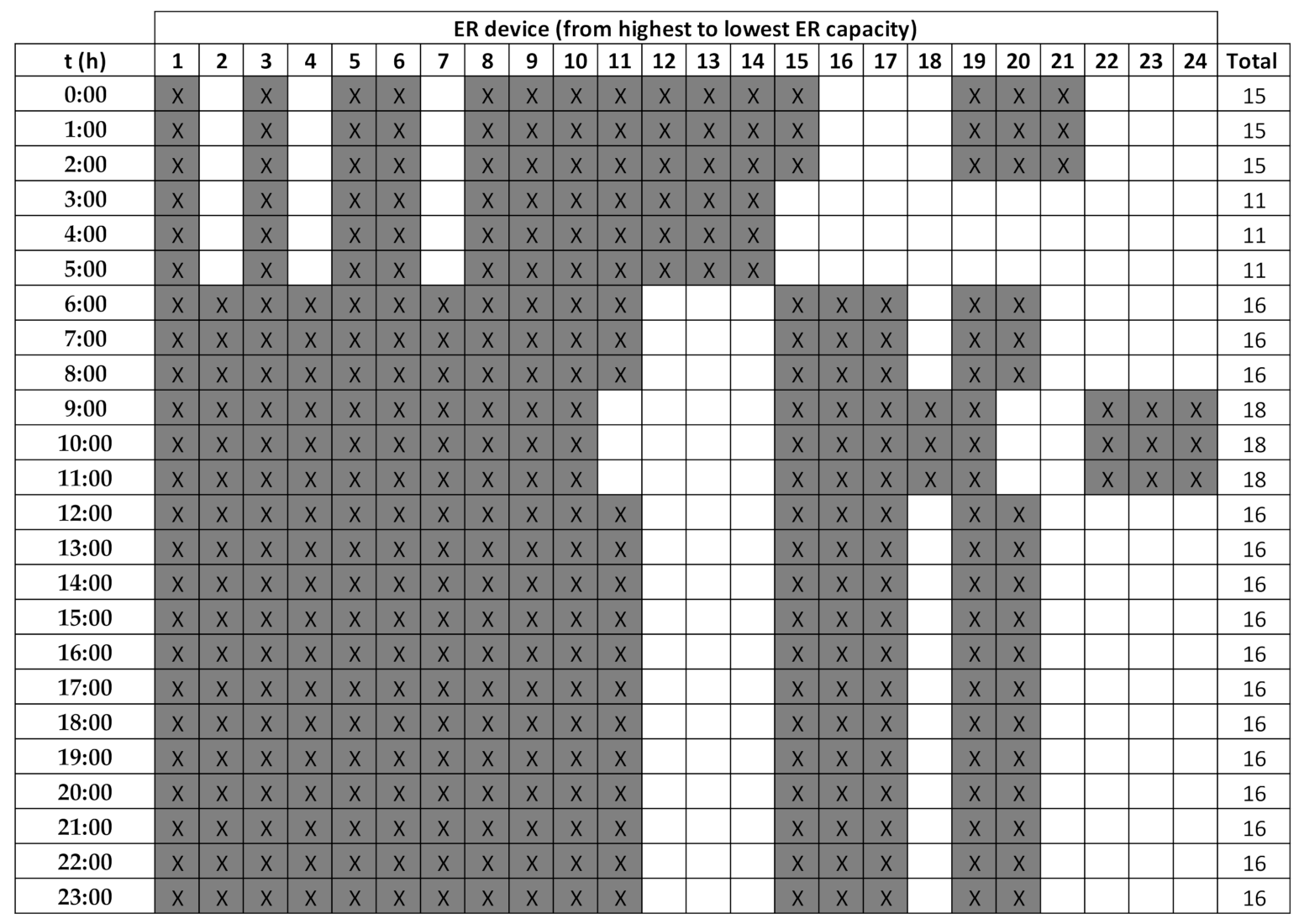
When the methodology is applied to networks with dynamic models, a series of results such as those in Table 4 are obtained at time step. The problem is the ER devices obtained in all cases are not the same at all time steps. Figure 5 shows the results obtained in the Anytown network. Each horizontal line of the figure represents the results in each time step. All the devices are represented vertically from highest to lowest energy recovery capacity. Each cell represents if the device of the column recovers energy at the instant represented by the line. If the device recovers energy, the cell is marked with an X, otherwise the cell is blank. Not all devices recover energy at all times. In fact, the number of ER devices varies from one instant to another, oscillating between 11 and 18. Something similar happens with the Net3 and C-Town networks.

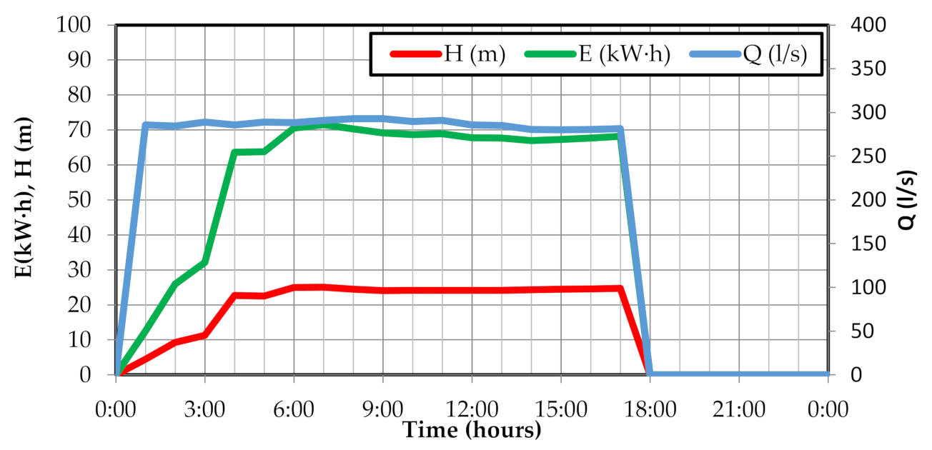
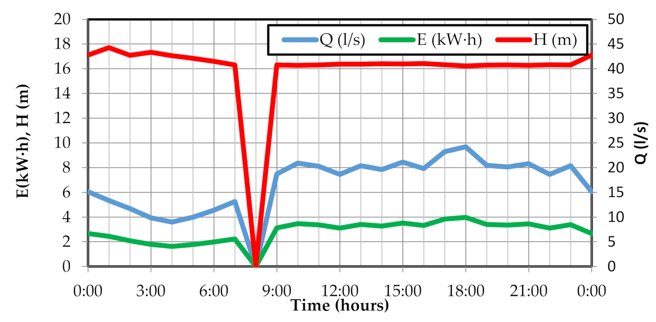
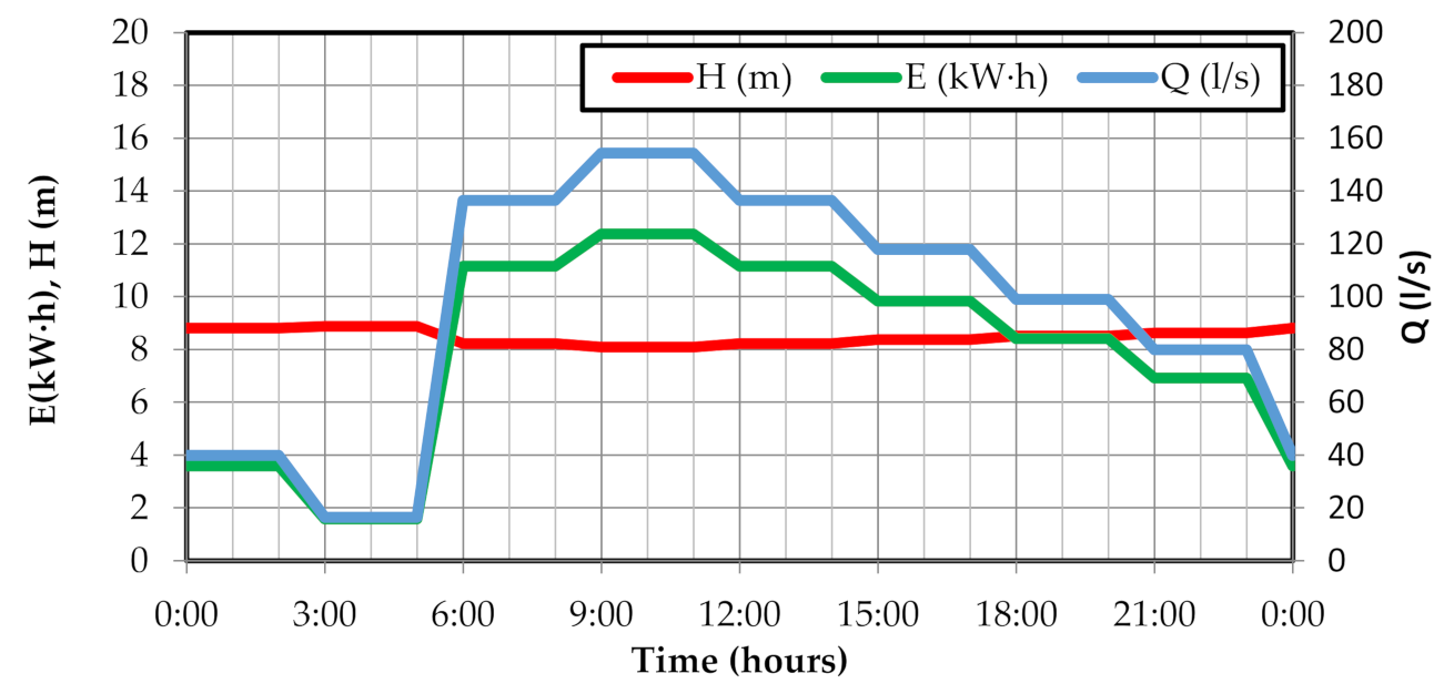
The ER capacity of devices varies over time. The following figures show the data obtained for the devices with the most ER capacity in the three cases (Anytown, Net3 and C-Town). In each of the graphs (Figure 6, Figure 7 and Figure 8) the red line represents the head (energy loss) of the ER device, the flow is represented in blue and the ER in green. Logically, the ER is directly linked to the flow. Although not in all cases, the device that recovers the most energy is active during all time steps. In the Net3 network, the device is disconnected from 18:00, while in C-Town the device is only disconnected only at 8:00.

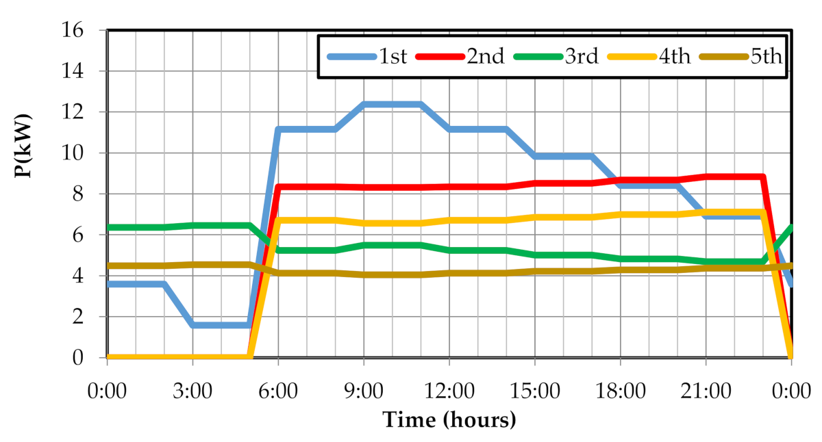
The results from the different devices vary over time. Figure 6, Figure 7 and Figure 8 show the energy recovered by the device with the highest capacity in each network. The variation in the device with the highest capacity is not maintained in the rest of the network devices. In each case, this variation depends on the topology and the specific characteristics of the network. 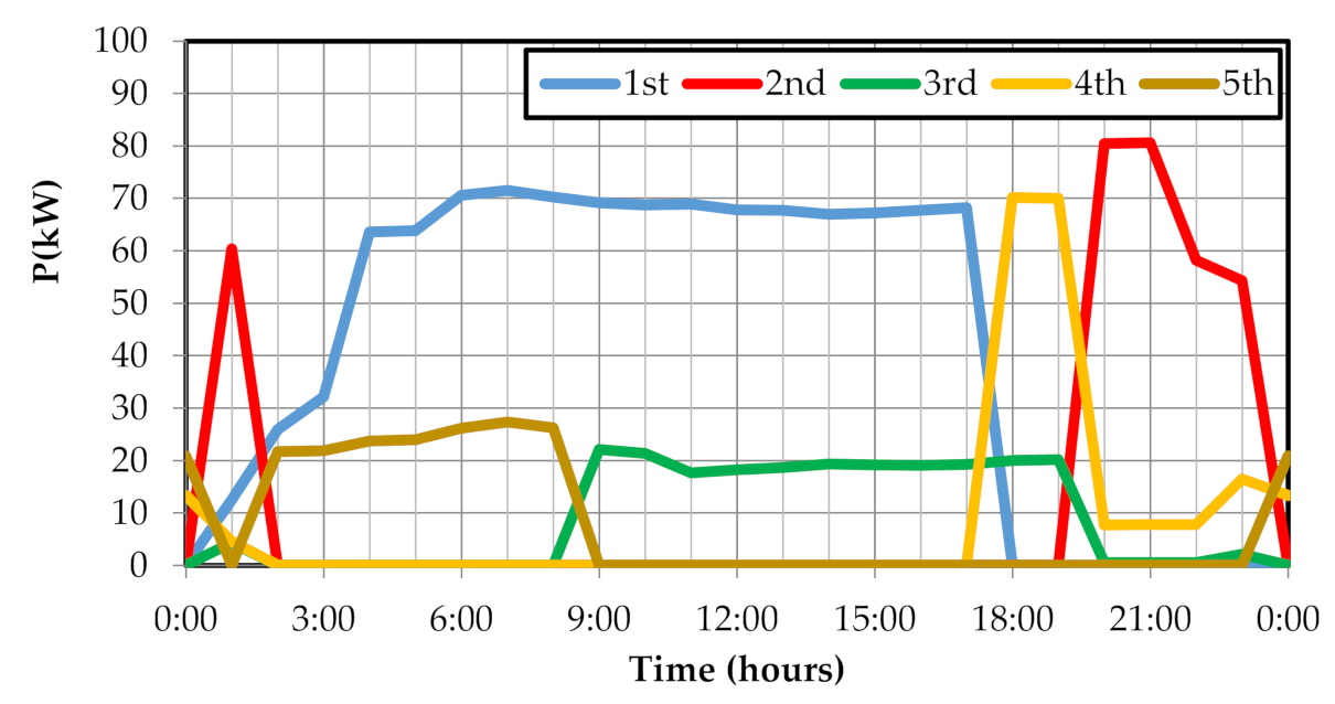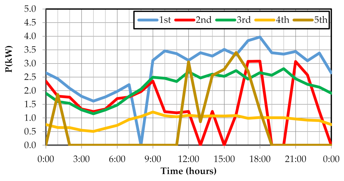Figure 9, Figure 10 and Figure 11 show the variation in the energy recovered in the five devices that recover the most energy.

The power recovered by each element (Figure 9, Figure 10 and Figure 11) varies with time. The PRE_n is obtained by integrating each device. In this way, a table similar to Table 4 of the Balerma network is obtained for each network. As in the case of the Balerma network the 6 devices with the highest capacity are collected (

Table 5. Results of 6 devices with the most ER in Anytown network.

No.	ID Link	ER (kW·h)	% ER	% Accum. ER
1	Pipe 80	195.01	18.43%	18.43%
2	Pipe 2	153.11	14.47%	32.91%
3	Pipe 12	129.93	12.28%	45.19%
4	Pipe 4	122.76	11.60%	56.79%
5	Pipe 6	102.53	9.69%	66.48%
6	Pipe 16	93.18	8.81%	75.29%

,

Table 6. Results of 6 devices with the most ER in Net3 network.

No.	ID Link	ER (kW·h)	% ER	% Accum. ER
1	Pipe 233	1022.69	38.60%	38.60%
2	Pipe 173	333.94	12.60%	51.21%
3	Pipe 191	223.07	8.42%	59.63%
4	Pipe 231	197.82	7.47%	67.09%
5	Pipe 193	191.85	7.24%	74.33%
6	Pipe 189	121.82	4.60%	78.93%

and

Table 7. Results of 6 devices with the most ER in C-Town network.

No.	ID Link	ER (kW·h)	% ER	% Accum. ER
1	Pipe P16	78.36	6.02%	6.02%
2	Pipe P794	15.85	5.19%	11.20%
3	Pipe P125	0.75	3.97%	15.17%
4	Pipe P142	4.31	3.87%	19.04%
5	Pipe P781	2.78	3.81%	22.84%
6	Pipe P758	0.48	3.57%	26.41%

). The rest of the values are included in the Supplementary Material.

4. Discussion

The application of the described methodology grants obtaining all the terms of the energy balance for the networks studied. Specifically, not only the PRE is achieved, but also the location of all the places where the installation of ER devices would lead to maximum ER.

Table 8. Summary of the application of the PRE methodology to the study cases.

Network	No. of Iterations			No. of ER Devices
	Min.	Max.	Total	Min.	Max.	Total
Anytown	2	3	72	11	18	24
Net3	11	23	401	11	40	66
C-Town	118	131	3093	135	157	190
Balerma	214			225

contains a statistical summary of the results gather after applying the methodology at the 24 time steps computed.

The results obtained at each instant for the networks analyzed using dynamic models differ. Therefore, the table shows the total number of iterations required and the maximum and minimum values of this number of iterations at the different time steps. It should be noted that the number and locations of the ER devices at diverse times may be different. For this reason, Table 8 shows the total number of different ER devices to be installed in order to achieve the maximum ER and the maximum and minimum number of ER devices. It must be emphasized that in the case of the Balerma network, a single value of iterations and ER devices is collected. Being a static analysis model, a steady state model is analyzed and therefore a single ER scenario is obtained.

The results of applying the methodology vary depending on the topology and the configuration of the network. However, there is a trend that clearly shows how the number of iterations and the number of ER devices required increases with the complexity of the network. Furthermore, the number of ER devices required is large.

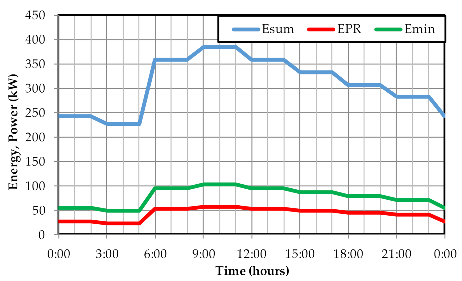
Another significant aspect obtained from the application of the methodology is the energy balance and the results of the PRE are different over time. If the network model considered is dynamic, there is a variation in circulating flows and pressure levels over time. This translates into a variation over time of the different terms that are part of the energy balance of the network. Figure 12 represents the results of the energy supplied (E_sum), the minimum energy required (E_min) and the PRE in the Anytown network. The values represented in Figure 4 are the power at each instant. The corresponding energy associated with each line would be the area enclosed under each of them. It can be seen how none of these values remains constant over time. Similar graphs can be obtained for the rest of the networks studied.

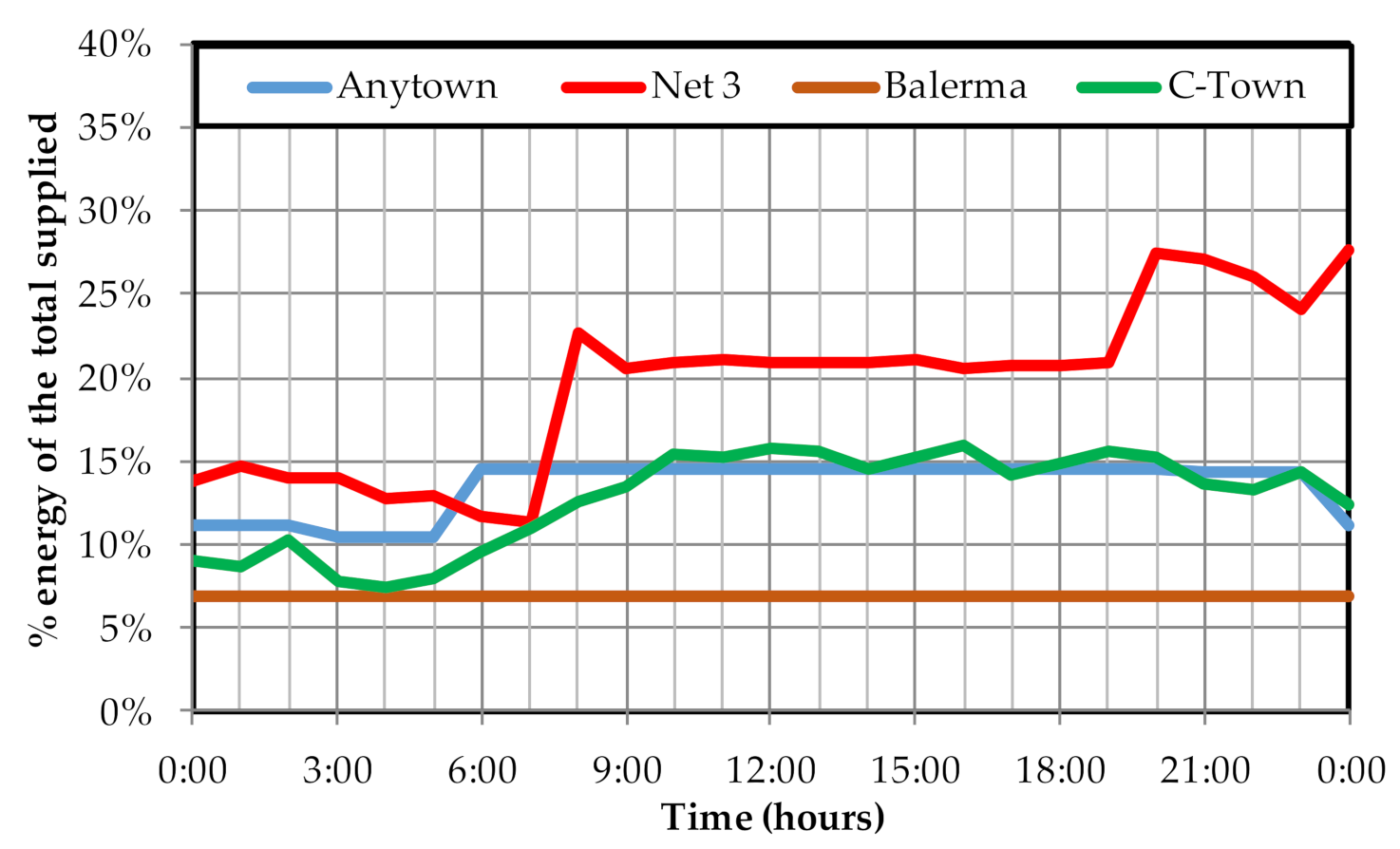
The analysis of Figure 12 shows a similar trend between supplied energy and PRE. Although it appears to be a certain correlation between them, the results show that the percentage of the PRE with respect to the total energy supplied is different. Figure 6 shows the percentage of PRE in the network elements (pipes and valves) with respect to the total energy supplied. This percentage is the relationship between the sum of the terms PRE_n and PRE_v with respect to the energy supplied (E_sum).

Figure 13 shows the evolution of the PRE percentage is different in each network. Note that the Balerma network is analyzed only in steady state. Consequently, it has been represented as a constant line. In the rest of the cases, the percentage is not constant and there are significant variations throughout the day. In the case of Anytown, the PRE represents an average of 13% of the energy supplied, with fluctuations of up to 5%. In the other networks, the mean values are somewhat higher (20% in Net3 and 13% in C-Town). Likewise, the oscillations of this percentage are also higher (14% in Net3 and 6% in C-Town). Ultimately, the variation of this percentage of PRE depends entirely on the configuration of the network, the temporal variation of its demands and its operation criteria.

A complete analysis of the ER in the networks is obtained when the results derived from the application of the methodology are analyzed not instantly, but by calculating the daily energy values. Therefore, the final results after obtaining the maximum PRE in the networks are shown in

Table 9. Energy analysis of the study cases (kWh).

				Anytown		Net3		C-Town		Balerma
Esup	Er		Er,r	2414.7	2414.7	11,284.2	12,018.4	3975.1	5058.4	1299.1	1299.1
			Er,t	0.0		734.2		1083.3		0.0
	Ep			5312.9	5312.9	2508.4	2508.4	5074.7	5074.7	0.0	0.0
Econ	Enr	Ed,r	Ed,f	1088.7	1088.7	5753.4	5753.4	2082.0	2082.0	330.1	330.1
			Ed,p	0.0		0.0		0.0		0.0
			Ed,v	0.0		0.0		0.0		0.0
		Ed,a	Ed,l	0.0	114.5	0.0	1005.2	0.0	1379.0	0.0	0.0
			Ed,t	114.5		1005.2		1379.0		0.0
	Eu	Emin	Eu,e	1971.0	3927.8	517.2	3902.9	2874.7	4162.2	616.3	832.9
			Eu,p	1956.8		3385.8		1287.5		216.6
		PRE	PREu	1538.8	2596.7	1215.8	3865.2	1132.2	2509.9	47.3	136.1
			PREn	1057.9		2649.4		1302.6		88.8
			PREv	0.0		0.0		75.0		0.0
	ER			0.0	0.0	0.0	0.0	0.0	0.0	0.0	0.0

. In this case, an energy balance similar Table 1 example has been made for each network.

The energy balance has been divided into two parts: the energy supplied and the energy consumed. The supplied energy is divided into the different terms defined in Equation (2). The initial hydraulic simulation of the network allows to obtain the total PRE of each network and the PRE in the control valves (PRE_v) existing in the network. Discrimination from the rest of PRE can only be done by applying the proposed methodology. This application allows to separate this remaining PRE into the energy that can only be recovered by users (PRE_u) from that which can be obtained from the network (PRE_n). The results collected in Table 9 refer to energy (kW·h) throughout the simulation time in the first three networks. In the case of the Balerma network, as it is a steady state analysis, the values collected are power at the instant studied, not energy.

The last line of Table 9 shows the ER in the network. The networks analyzed do not initially have any ER device. For this reason, the E_R value in this table is null. In the case of installing a certain ER device in the network, the value of the recovered energy would be discounted from the row of PRE_n or PRE_v (depending on whether it is installed in a pipeline or if it replaces a control valve). At the same time the E_R row would increase by a value equal to the one previously discounted.

A more detailed analysis of the energy balance of the networks after applying the ER methodology is shown in

Table 10. Summary of the PRE and the main energies in the study cases.

	Anytown	Net3	C-Town	Balerma
En,r	15.6%	46.5%	34.2%	25.4%
Emin	50.8%	26.9%	41.1%	64.1%
PRE	33.6%	26.6%	24.8%	10.5%
PREu	19.9%	8.4%	11.2%	3.6%
PREn	13.7%	18.2%	12.9%	6.8%
PREv	0.0%	0.0%	0.7%	0.0%

. This table shows different percentages of energy with respect to the total energy supplied or consumed. The first three lines represent the non-supplied energy (E_n,r), the minimum energy necessary (E_min) to guarantee the supply and the PRE without discriminating between which part can be recovered in the network and which part can only be recovered by users. The final three lines make the percentage breakdown of the PRE, dividing it into its three components: PRE_u, PRE_n and PRE_v.

A first analysis of the results of Table 10 shows the PRE decreases with the level of complexity of the network. Unless the network has an abrupt topography or very varied pressure levels, the ER capacity of the network is progressively diminished with increasing complexity. In the case of the Balerma network, an extremely low value (10.5%) of the PRE is obtained. This low value is due to two circumstances. First, the Balerma network has been optimized many times, so its solution can hardly be improved. Second, it is a steady state analysis. Undoubtedly, the presence of excess energy in a network optimized for a single instant of time is easier than optimizing a network for operation over time. Hence, Balerma’s solution allows less ER capacity than the rest of the networks.

In terms of the discrimination of the total PRE, there is no rule or a clear trend, since it depends on the configuration of the network. Due to the characteristics of the networks, only C-Town presents PRE_v in a value that barely represents 3% (0.7% of 24.8%) of the PRE in the network. Regarding the discrimination between PRE_n and PRE_u, there is no clear relationship with the size of the network. The percentage of PRE_n with respect to the total PRE ranges between 40.7% (Anytown) and 68.5% (Net3). In any case, the application of the proposed methodology makes it possible to appreciate that a large percentage of the excess energy in the network is not recoverable due to its own topography. The minimum energy requirements in some critical points of the network force to have excess pressure in other points. Said energy surpluses (excess pressure over the minimum required) are necessary to guarantee that the supply conditions are met at critical points.

The objective of this work is not the determination of the number and location of ER devices more appropriate to install in a network. This is a problem that requires defining an economic objective where all investments are economically valued. The objective of this work was to determine the maximum PRE of a network without modifying the flow distribution. However, it is interesting to discuss the results obtained to analyze the influence of the number of installed devices.

In general terms, it can be concluded that the number of devices required for the recovery of the maximum PRE is very high. That is, a very high percentage of the lines in the model compel the installation of one of these elements. Thus, in Balerma it is necessary to install these devices in 49.6% of the pipes (225 out of 454). Something similar happens in the rest of the networks: 60.0% in Anytown, 58.8% in Net3 and 41.1% in C-Town. This does not mean that all these devices are economically profitable, but rather that they represent the total of devices required to obtain the maximum energy recovery in the network. However, a detailed analysis reveals that the energy recovery capacity of the devices is very different. Generally, a few devices can recover a large part of the energy, while many of the devices hardly contribute to the overall energy recovery. 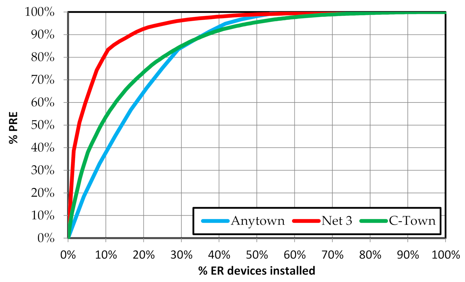This is especially evident in the results of Figure 14.

This figure represents the percentage of recovered energy with respect to the maximum PRE_n as a function of the percentage of the installed devices. Specifically, installing around 10% of ER devices, the percentage of recovered energy obtained is different. In Anytown, the installation of three devices (12.5% of the total) allows to recover 45% of PRE_n. On the other hand, in Net3 the installation of seven devices (10.6% of the total) allows to recover 83.4% of PRE_n. Finally, in C-Town 10 of the 19 devices with the highest capacity (10% of the total) allow to recover only 53.6% of the PRE_n.

In the same line, to recover around 80% of the PRE_n, the number of devices is also very different. In the Anytown case, seven devices are required (29% of the total) to recover 83% of the energy. In Net3, the same number of devices is required for the same percentage of ER. However, in Net3 these seven devices represent only 10.6% of the total number of devices that lead to the maximum PRE_n. Finally, on the C-Town network, 48 devices are required (25% of the total) to reach 80% of the maximum PRE_n. In short, obtaining the number of devices to install will depend on the results of this work and a benefit-cost analysis.

The results derived from the application of the PRE_n calculation method allow filling in energy balances such as the one shown in Table 9. From the detailed balance of each network, it is possible to evaluate the proposals for resilience indices. The results compared with the proposed indices with the Todini resilience index are shown in

Table 11. Summary of the indicators calculated for the studied networks.

Network	Anytown	Net3	C-Town	Balerma
IEE	0.863	0.818	0.864	0.932
PREI	0.407	0.685	0.549	0.653
RI	0.683	0.364	0.420	0.292
PREIstd	0.278	0.249	0.231	0.191

. The table shows the energy efficiency index (I_EE) calculated according to Equation (5), the Todini resilience index (RI), and the PREI defined in (6). Additionally, in order to establish some comparisons, a standardized PREI (PREI_std) has been defined. PREI_std has the same definition as the PREI, but the denominator has been replaced by the excess energy supplied Todini uses in its definition of the RI.

The calculation of the I_EE index requires the results of the application of the ER methodology, since it is necessary to determine the values of PRE_n and PRE_v. As can be seen, the I_EE of the Balerma network is significantly higher (0.932) than the rest of the networks. Again, this is because the network has been analyzed in steady state and is already an optimized network. The rest of the networks present lower energy efficiencies because they are analyzed with an extended period simulation model.

In general, the I_EE only shows the energy efficiency of the network. Thus, from the energetic point of view high values of I_EE indicate the network operation is highly optimized. However, when the values of excess pressure at the nodes refer to excess energy supplied, this relationship is not so clear. This deepens the need to define two different indices: one to analyze the energy efficiency of the network and the other to analyze its energy recovery capacity. This is main contribution of the PREI: marking the ER capacity in a network. It is therefore an index that depends a lot on the configuration of the network and its original design. Thus, the Balerma network, a very efficient network (high I_EE value), also presents a high PREI value. This is because the PREI indicates the fraction of the excess energy that is recoverable. Therefore, although this network has low excess energy, a large part of this excess is recoverable in the network. On the contrary, a network like Anytown with lower energy efficiency (0.863) would potentially have more excess energy. However, due to its configuration, Anytown has a lower energy recovery capacity (PREI value 0.407). In short, both indexes are complementary.

The PREI can be used not only as an indicator of efficiency in ER but also as an indicator of network resilience. For this reason, Table 11 shows two more indicators. The first is the RI of Todini, which represents the excess energy supplied at the nodes with respect to the minimum energy required. In the networks analyzed, Balerma presents the lowest resilience value (0.292, the lower RI value) since it is a much more optimized network than the rest. The RI, initially defined as an indicator of resilience, represents at the same time a simplified energy balance of the network. The only restriction of this index as an energy indicator is that it does not take into account the topology of the network. That is why in the same Table 11 a modification of the PREI is defined. This has been called the standardized PREI (PREI_std), which includes in the numerator the same terms as the PREI but the same excess energy in the denominator as the RI.

The analysis of the results in Table 11 indicates that the PREI_std is always lower than the RI. This indicates that a part of the excess energy in the RI energy balance cannot be recovered due to the topography of the network.

To understand the differences between RI and PREI_std, it is enough to consider a network with two nodes fed from a tank. Consider the critical node is the one at the end. To achieve the minimum pressure at the end node, excess pressure is required at the intermediate node. In the case of the RI, this energy excess over the minimum required is a certain resilience capacity of the network, since the RI only measures excess pressure over the minimum. In the case of the PRE calculated in this work, this excess energy would be PRE_u since it could only be used by the users connected to the node. However, the PRE_n calculation method in this network assumes a null value. Consequently, the PREI_std collects a null value since the network does not have ER capacity. In short, the application of the PRE_n calculation method leads to applying more real resilience indices. Excess pressure in nodes where the pressure cannot be reduced does not imply a greater resilience of the network.

The index PRE_std could be itself a good energy or resilience indicator. However, PRE_std can be approximated in all networks as the product of the RI and the PREI, so considering the first two, the explicit definition of a third indicator does not make sense.

5. Conclusions

The energy analysis of a WDN is important. This importance is proofed the various energy balances that can be found in the scientific literature. Furthermore, a few studies examined the hydroelectric potential of a WDN, but none of them were able to quantify the maximum PRE in detail. The lack of knowledge of the energy recovery potential of WDNs means that many of the ER decisions are made without taking into account a global assessment of the problem. Numerous problems address ER in WDN, but so far, no work could methodologically quantify the maximum PRE. Knowledge of this maxim PRE is essential as a measure of any ER strategy in WDN, to reduce energy consumption and to define the possible locations of ER devices.

For this reason, in this work a new energy balance of a WDN is proposed. This new balance provides useful information to distinguish all possible energy losses that may occur in the network, allowing not only to show the status of the network but also to measure the excess energy. Some of the existing energy balances deal with PRE, but none goes into the detail of how this PRE is distributed in a WDN. Therefore, it was necessary to calculate the existing PRE in a methodical way: the PRE that comes from replacing the existing control valves with microturbines or PATs, the PRE that comes from installing new ER devices in the network and the PRE that can only be recovered by the network users in their private facilities. Once the energy balance of a WDN has been defined, the hydraulic analysis of the network allows calculating both the PRE and PRE_v. Therefore, it was only necessary to calculate the PRE_n to have the balance completely defined, since the PRE_u is defined by the difference between the PRE and the terms PRE_v and PRE_n.

The determination of PRE_n requires a methodology such as that described throughout the work. It is an iterative method in which it is assumed that the flow rates in the lines will remain constant before and after the ER. From there, a methodology such as the one defined schematically in Figure 3 is proposed. The method for ER is carried out by applying it to an example network as indicated in Figure 4. In this way, the method appears as a compact algorithm that considers the different operating modes of a WDN (pumping supply, gravity feed, presence of control valves, installing of ER elements). In short, it is a complete methodology that finally leads to the evaluation of the maximum energy that can be recovered in the network by installing the appropriate ER devices (PRE_n). Undoubtedly, the PRE_n calculation allows completing the rest of the energy balance of the network, and constitutes, together with the proposed energy balance, the two main contributions of this work.

The methodology to determine the PRE demonstrates its validity as it has been applied to four different study cases. There are four WDNs of different sizes, one with a steady state model and three with an extended period simulation model. Obtaining the PREs and their discrimination between PRE_u and PRE_n is fast since the number of iterations is not excessive. Additionally, the method allows finding the location of the ER devices.

Obtaining the PRE_n and PRE_v values has made possible to define two energy indices: the I_EE and the PREI. The first one has been shown as an indication of the energy efficiency of the network since it is capable of assessing the use that the network makes of the energy consumed. The second one (PREI) is more oriented to ER. It is an indicator of the percentage of excess energy that can be recovered. This indicator (PREI) does not assess the totality of energy that can be recovered, but rather the capacity of the network to recover energy. For example, a network with a high I_EE value will have low PRE value. In that case, a high PREI value would indicate that a high percentage of the total PRE can be recovered, but even so, it continues to be little the PRE, since the excess energy is very small.

This limitation of the valuation of the excess energy of the PREI is what has made the PREI complement the Todini’s RI. The RI, in addition to an indicator of resilience, is an indicator of excess energy in the network. In fact, the product of both (PREI and RI) is what in this work has been called PRE_std, which is really the indicator of the ER capacity of the network. That is, it is an indicator of the percentage of the total energy that can be recovered in the pipes (by installing ER devices) or in the valves (by replacing them with microturbines or PATs). Ultimately, the developed method leads to a new way of evaluating energy in WDN with emphasis on PRE.

As can be seen in the results of the analyzed networks, the method leads to the definition of numerous points where an ER device could be installed. However, this does not mean that all of them are energetically or economically viable. The method allows obtaining the maximum ER, the location of all the possible ER points and the value of the energy to be recovered in each of them. Some of them may have a very low ER. In addition, it is possible that not installing some ER devices with small capacity would allow other devices to have higher ER capacity. This is one of the limitations of the current methodology. The method does not carry out a global optimization, nor does it discriminate about the points where the installation of energy recovery units would be more profitable. Just look for the maximum PRE.

Finally, it is worth highlighting the limitation derived from considering the invariability of the flows before and after ER. This hypothesis has remained fixed throughout the work. That is why this work has two fields of future development. The first would be to extend the methodology to the case of models in which consumption is dependent on pressure. In this case, the invariability hypothesis of the flows might not be adequate. The second would be to explore other energy recovery solutions that could generate less energy but concentrate it on smaller ER devices.