Assessing the Feasibility of a Cloud-Based, Spatially Distributed Modeling Approach for Tracking Green Stormwater Infrastructure Runoff Reductions

Abstract

Use of green stormwater infrastructure (GSI) to mitigate urban runoff impacts has grown substantially in recent decades, but municipalities often lack an integrated approach to prioritize areas for implementation, demonstrate compelling evidence of catchment-scale improvements, and communicate stormwater program effectiveness. We present a method for quantifying runoff reduction benefits associated with distributed GSI that is designed to align with the spatial scale of information required by urban stormwater implementation. The model was driven by a probabilistic representation of rainfall events to estimate annual runoff and reductions associated with distributed GSI for various design storm levels. Raster-based calculations provide estimates on a 30-m grid, preserving unique combinations of drainage factors that drive runoff production, hydrologic storage, and infiltration benefits of GSI. The model showed strong correspondence with aggregated continuous runoff data from a set of urbanized catchments in Salinas, California, USA, over a three-year monitoring period and output sensitivity to the storm drain network inputs. Because the model runs through a web browser and the parameterization is based on readily available spatial data, it is suitable for nonmodeling experts to rapidly update GSI features, compare alternative implementation scenarios, track progress toward urban runoff reduction goals, and demonstrate regulatory compliance.

1. Introduction

The continued expansion of impervious cover disrupts natural hydrologic cycles, increasing runoff from storms [1], which enhances the entrainment and transport of sediment, nutrients, bacteria, metals, pesticides, and other pollutants [2,3]. Municipalities throughout the United States are required to implement structural and nonstructural controls, known as best management practices (BMPs), to reduce runoff and urban pollutant loading to receiving waters. BMPs are a key component of low impact development and increasingly include small-scale green stormwater infrastructure (GSI) such as infiltration or bioretention features widely distributed throughout the urban landscape. Where traditional “grey infrastructure” uses engineered hard structures, GSI uses plants, soils, and landscape design to reduce runoff and pollutant entrainment close to where rain falls to restore the natural hydrologic functioning of urbanized landscapes. GSI has become increasingly popular as a cost-effective way of reducing pollution from urban stormwater pollution [4]. The well-documented co-benefits of GSI include water quality improvements [5], reduction of local flooding risks [6,7,8], recharging groundwater [9,10], and climate change impact mitigation via carbon dioxide uptake [11,12] and reduction of the urban heat island effect [13].

While site-scale effectiveness of individual BMPs has been widely documented [14,15,16,17], there is little compelling evidence available via measurements or modeling of improvements resulting from distributed GSI implementation at urban catchment scales (e.g., 1–1000 km²) [18]. While a few recent studies have begun to build this understanding via field measurements [4,19,20] and modeling [21,22], the effectiveness results are mixed [17] and substantial uncertainty remains for how implementation may scale up to catchment-scale changes over the long term [23,24]. The uncertainty is largely because the high variability associated with storm flows obfuscates the signal of hydrologic or water quality changes associated with stormwater management activities [25]. Monitoring designs that minimize sources of variance with long time series and precise measurements in areas with relatively intensive GSI implementation have the best chance to draw causal linkages between GSI implementation and catchment-scale hydrologic changes [17], but data resulting from such efforts are scant.

Given the high costs of monitoring, municipal stormwater programs must often rely on modeling tools to estimate the levels of GSI implementation needed to reach water quality milestones [26]. A trade-off between greater resolution in space or time is generally required and reflected in the chosen model structure, since granular representation of both is excessively complex and computationally expensive [27,28]. Greater process representation complexity does not necessarily improve model utility, especially when information to constrain model behavior is severely limited [29,30]. Recent work illustrates that the location and spatial distribution of GSI practices can be a key factor in catchment-scale effectiveness [18,20,25]. Since stormwater planning decisions are often made at the scale of parcels, high spatial resolution models with simplified processes may provide more useful outputs compared to models with detailed process representation but lower spatial resolution. In this study, we present an updated version of the Stormwater Tool to Estimate Load Reductions (swTELR), previously reported by Beck et al. (2017) [31], which employs a parsimonious parameterization to align with spatial data sets that are commonly available to cities. While the previous version of the model made calculations at the urban catchment scale (approximately 40–100 ha) for quantifying centralized stormwater treatment, this version uses 30-m (0.09-ha) grid-scale calculations to facilitate spatially explicit representation of small-scale GSI BMPs throughout a city. This approach allows a hierarchical drainage configuration so that reductions from distributed GSI can be nested within drainages treated by larger centralized BMPs. Thus, it provides an efficient way to scale up runoff reduction accounting that preserves site-level characteristics, linkages between BMPs, and connectivity between drainages. The purpose of the model improvements is two-fold: (1) provide a means for identifying high priority opportunity areas for future GSI implementation and (2) allow tracking of catchment scale, GSI-driven runoff reductions over time by nonmodeling experts at multiple scales. The model runs via a web browser and is implemented using cloud-based raster processing to facilitate use by wider audiences, a key technical deficiency for current GSI modeling tools [32].

In this paper, we present the cloud-based implementation of the analytic framework and describe the web interface that allows stormwater program managers to run simulations and update inputs, such as GSI projects and BMP specifications, as stormwater programs adjust practices over time. We present the model formulation along with results of initial catchment-scale baseline condition verification experiments and discuss how ongoing use with monitoring data can provide a strong basis for testing catchment-scale GSI effectiveness for reducing stormwater runoff and pollutant loading.

2. Methods and Data

2.1. Model Scales of Representation

Typically, stormwater runoff is modeled using one of two approaches: using discrete storm events or continuous simulation. Event-based approaches are programmatically simple but were originally designed to simulate runoff for a single storm event size. With swTELR, we employed a hybrid event-based approach that combines a set of events drawn from a long-term precipitation distribution to bracket the range of rainfall and runoff responses probabilistically (as opposed to explicitly with continuous simulation). The efficiency of this method allows a distributed spatial approach where runoff, loading, and BMP reduction calculations are discretized on a 30-m grid so that site-specific runoff generation and pollutant loading characteristics specific to the BMP drainages are explicitly represented. This also allows derivation of the model parameterization from widely available spatial data sets, rather than a calibration process that requires flow data that are typically unavailable at urban catchment scales. Since GSI runoff reductions typically occur very close to the runoff generation source, flow timing across grid cells along with hydraulic factors are assumed to be nominal and not represented in the model.

2.2. Rainfall Calculations

Stormwater TELR calculates various 24-h precipitation depths and the average annual number of days with measurable precipitation to represent the overall distribution and total average annual depths. We calculated d, the average number of rain days per water year when daily rainfall exceeds 0.25 cm, and P(x), various 24-h event frequency estimates, where P is the 24-h rainfall depth for the xth percentile event. On a water-year basis, we selected 24-h event rainfall frequencies to approximate the 24-h event cumulative distribution function, such that these events can be summed to obtain long-term average 24-h runoff volumes for days when it rains:

$${{\displaystyle \int }}_0^{100}P\left(x\right) dx\approx \frac{1}{2}{\sum }_{k=1}^N\left(x_{k+1}-x_k\right)\left(P\left(x_{k+1}\right)+P\left(x_k\right)\right)$$

(1)

where x is a number between 0 and 100 and k is number in the sequence of total, N, percentile events used to estimate the integral. With this formulation, long-term average annual rainfall depth, P₃₆₅, is the product of the integrated 24-h rainfall depth and the number of rain days per year, d:

$$P_{365}= (d)P\left(x\right)dx.$$

(2)

This approach to characterizing the long-term precipitation distributions was compared with several other approaches by Beck et al. (2017) [31]. Runoff and decentralized BMP reductions are calculated using the individual percentile rainfall events that correspond with common water quality permit requirements and structural BMP design criteria (85th and 95th percentile storm events), which also include the median and the lower quartile.

2.3. Rainfall–Runoff Transformation

For a given storm magnitude, the runoff generation module defines the fraction of flow that infiltrates over pervious surfaces and the fraction of overland runoff that is eventually discharged to the receiving waters or existing stormwater infrastructure. Stormwater TELR relies on the Natural Resources Conservation Service (NRCS) curve number (CN) method and the approach detailed in Technical Release 55 (TR-55) to estimate runoff from small urban catchments [33]. The NRCS runoff equation is:

$$Q=\frac{{\left(P-I_a\right)}^2}{\left(P-I_a\right)+S}$$

(3)

where Q is the runoff depth, P is the 24-h rainfall depth, S is the potential maximum retention after runoff begins, and I_a is the initial abstraction depth, which incorporates all losses before runoff begins, including water retained in surface depressions, water intercepted by vegetation, evaporation, and infiltration. Runoff does not begin until the initial abstraction has been met. I_a is variable across the landscape but is highly correlated to the curve number. The initial abstraction is 20% of the storage,

$$I_a=0.2S$$

(4)

and

$$S_{0.20}= \frac{1000}{CN}-10.$$

(5)

More recent data suggest that 0.20*S might be too high and that 0.05*S is more appropriate [34,35,36] especially for soils with lower infiltration rates [37]. If 5%, rather than 20%, is used, S must also be modified. The relationship between S_0.05 and S_0.20 obtained from model fitting results is [35,38]

$$S_{0.05}= 1.33S_{0.20}{}^{1.15}.$$

(6)

We used the adjusted initial abstraction ratio (Equation (6)) and by substituting Equation (4), modified for 5% of storage, into Equation (3), we obtained:

$$Q=\frac{{\left(P-0.05S_{0.05}\right)}^2}{P+0.95S_{0.05}}.$$

(7)

Thus, the model was parameterized by specifying the curve number, which ranged from 30 to 98, with lower numbers indicating low potential runoff and higher numbers indicate increasing runoff potential. The major factors that determine NRCS curve numbers are the soil type, the land use (specifically, the percent impervious of the land use), the hydrologic condition, and soil infiltration capability. To simply account for variations in soil permeability and infiltration, the NRCS has classified soils into four hydrologic soil groups denoted by the letters A, B, C, and D. A curve number for a given land use with impervious area can be estimated by the following [33]:

$$CN= C{N}_p+\frac{P_{imp}}{100}\left(98-C{N}_p\right)$$

(8)

where CN is the runoff curve number for the entire land use, CN_p is the pervious runoff curve number, and P_imp is the percent of imperviousness. The pervious curve numbers used were those defined for open space in poor condition (grass cover < 50%) [33], since urban soils are often disturbed or compacted, and are listed in

Table 1. Urban pervious curve numbers used in the Stormwater Tool to Estimate Load Reductions (swTELR) derived from United Stated Department of Agriculture (USDA, 1986) [33].

Soil Type	A	B	C	D
Starting Curve Number	68	79	86	89

.

2.4. Runoff Reduction Accounting

Decentralized BMP runoff reductions are calculated based on their design storm specifications and spatial factors affecting runoff generation within the BMP drainage. All runoff generated up to the design storm depth infiltrates into the ground or evaporates, while flows generated above the design capacity are bypassed and routed downstream. For example, if a BMP is designed to the 85th percentile rainfall event, all runoff generated from events up to and including the 85th percentile event will be infiltrated. Similar to the rainfall approximation, integration of total flow reductions from decentralized BMPs are calculated via a Riemann sum of the flows generated by each rainfall event up to the x^th percentile using the trapezoid rule from each, per Equation (9):

$${{\displaystyle \int }}_0^{100}Q\left(x\right) dx \approx \frac{1}{2}{\sum }_{k=1}^N\left(x_{k+1}-x_k\right)\left(Q\left(x_{k+1}\right)+Q\left(x_k\right)\right)$$

(9)

where Q is the treated runoff volume for the xth percentile design storm, x is a number between 0 and 100, and k is a number in the sequence of total, N, percentile events used to estimate the integral. Flows from rainfall events larger than the xth percentile storm are partially treated, up to the xth percentile depth. Annual flow reductions (Q₃₆₅) are estimated as the product of the integrated 24-h flows and the number of annual rain days, d.

$$Q_{365}= (d)\int Q\left(x\right)dx$$

(10)

The total runoff volume treated is estimated as the sum of the direct runoff generated from each 30-m grid cell within a decentralized BMP’s drainage area,

$$Q_{365d}=Q_{1 }+Q_{2 }\dots + Q_{i }$$

(11)

This provides a computationally efficient way to account for reductions from thousands of BMPs throughout a city, which is independent of specific BMP design characteristics, as long as their design-storm depth specification is reliable. Such specifications are usually explicit in municipal National Pollutant Discharge Elimination System (NPDES) permits, along with standardized sizing guidance for different BMP types that rely on infiltration as the primary means of stormwater treatment, rather than filtration or particle settling. The resulting outputs are estimates of average annual runoff volume that can be summarized at multiple scales from the gridded data.

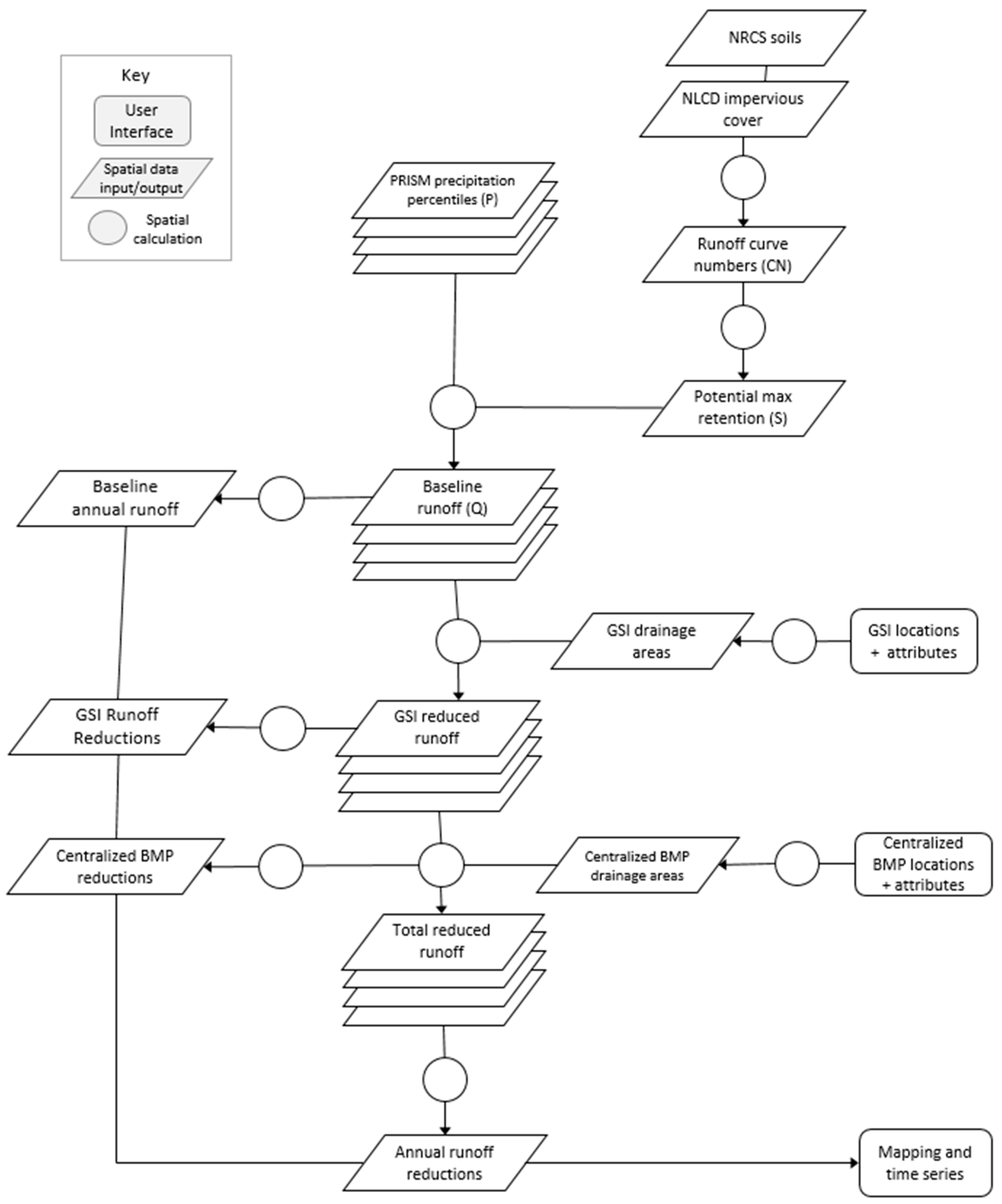
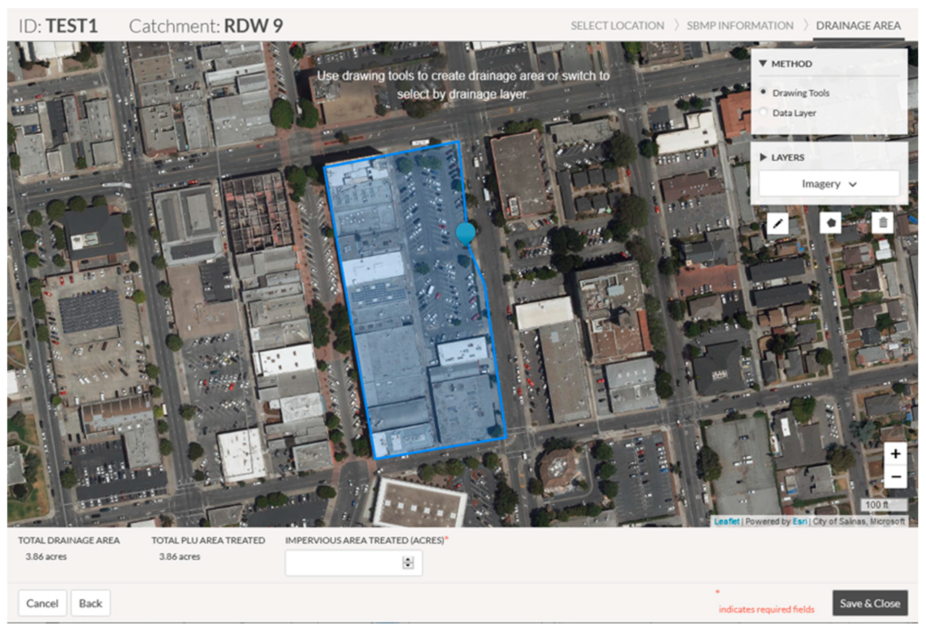
2.5. Model Structure and User Interface

The basic model structure is shown in Figure 1, with elements of the user interface, spatial data layer inputs and outputs, and calculation nodes. Runoff moves sequentially from areas of GSI treatment to centralized treatment if such BMPs are implemented so that spatial drivers of runoff reductions are reflected explicitly in the final outputs. Several raster layers that correspond to percentile values along the cumulative rainfall and runoff distributions are retained throughout the calculations, so that each process handles several events. The discrete events are combined via Riemann sums to produce interim and final output runoff layers. The web-based user interface provides a means for nonmodeling experts (e.g., a typical city stormwater manager) to update the model with new information on BMP installation as it becomes available, where users specify BMP locations, types, sizing, performance condition, and drainage areas. Users define the precise drainage area for each BMP, adding additional BMPs as they are implemented over time. Mobile apps allow field verification of BMP inventories and performance, with the data synced directly to the cloud. Raster calculations used for baseline runoff and reductions’ calculations employ scripts built in R and Python, while the user interface and input data handling employ PHP, GeoServer, PostgreSQL, and PostGIS. The open source stack has provided a cost-effective and flexible development environment for deployment to cities, and cloud-based analytics provide ready access to data and outputs from any location.

2.6. Input Data

Raster-based rainfall estimates from the PRISM Climate Group (2004) [39] at Oregon State University were used to describe the distribution of 24-h event depths to drive runoff generation. A script written in R using functions in the raster package [40,41] was used to acquire daily rainfall raster layers for the years 1981–2016 for the study area and perform the series of processing steps outlined in Section 2.3. The 35-year daily sequence (12,775 raster layers, 800-m² cells) was used to create a raster coverage of rainfall percentile values and average annual days of rain for each grid cell. Soils’ data from NRCS was used to specify soil types throughout Municipal Separate Sewer System (MS4) boundaries, used in their rasterized form, downscaled to 30-m pixels. The NRCS Soil Survey Geographic (SSURGO) database was used as the primary data source, and the State Soil Geographic (STATSGO2) database (which provides coarser resolution) was used to fill in spatial gaps in coverage that occur in the SSURGO data. Impervious cover was specified using the most recent data from the National Land Cover Dataset, which was provided at 30-m grid cell resolution [42].

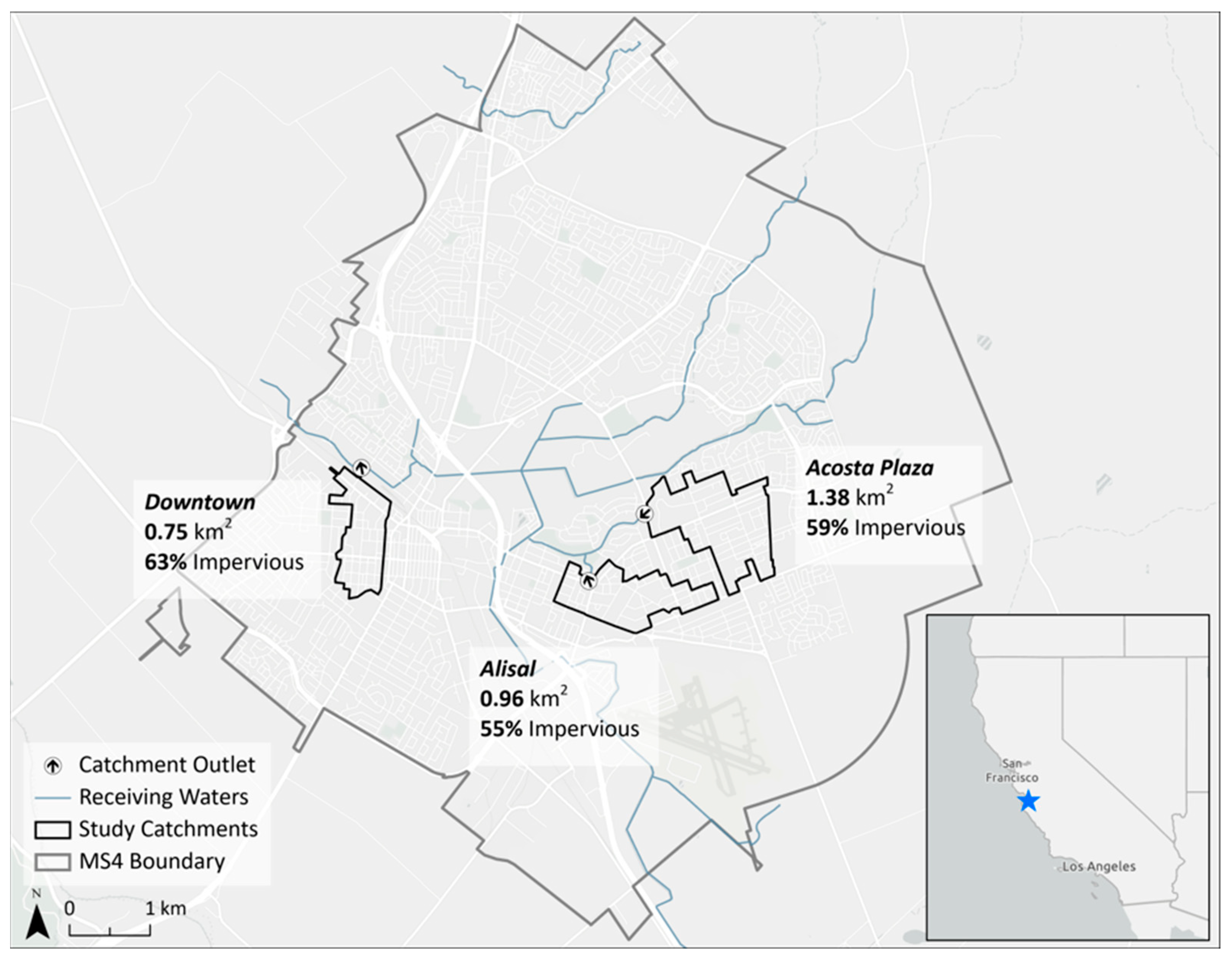
2.7. Study Catchments

A set of three urban catchments within the City of Salinas, CA, were instrumented with continuous stage recorders at their outlets for comparisons with the swTELR model (Figure 2) over a three-year period for water years (WY) 2018–2020. Located on the Central Coast of California, Salinas has a Mediterranean climate with nearly all of the precipitation delivered during winter months during a typical year (October–April). The catchments range in size from 0.74 km² to 1.4 km², are intensively developed, and are comprised of single-family residential, multi-family residential, commercial, and industrial land uses. Catchments were defined by surface drainage and the storm drain network, which had been mapped by Salinas municipal staff, which ensured that the area of runoff generation estimated in the model matched the contributing area of the catchment outlets. The Salinas storm drain infrastructure is separate from the sewer system, so that discharge measured at the outlets only reflects runoff from city streets and other urban landscape surfaces.

2.8. Comparison with the Catchment-Scale swTELR

We compared outputs from the grid-based version of the model with the catchment-based version previously reported by Beck et al. (2017) [31]. The primary difference between these two models is the scale at which they handle inputs and perform calculations: lumped at approximately 40 ha in the catchment-based model and 30 m in the grid-based model. Local rainfall gauge data were used in the catchment-based model, while the PRISM data were used for the grid-based model, with outputs aggregated to catchment level for the comparisons.

2.9. Monitoring Data and Model Comparisons

While there has been very little GSI to date in these areas of Salinas, they have been identified as priorities for intensive GSI implementation and, as such, provide a prime opportunity for understanding the measurable effects of GSI on runoff generation at this scale. At each catchment outlet, continuous stage was recorded at 10-min intervals and the data were regularly downloaded and converted to discharge estimates (Q) via Manning’s Equation [43]:

$$Q=\frac{1}{n}A{R}^{2/3}{S}^{1/2}$$

(12)

with hydraulic radius (R), slope (S) specified from field measurements and the roughness coefficient (n) specified from table values for the appropriate pipe material. Manual stage measurements were taken periodically at the outlet for calibration and quality assurance of the continuous measurements. Discharge volume was measured several times during the first year of monitoring to verify accuracy of the volume estimation method. Since there is not a permanent weir installed at these outfalls, these verification measurements could only be safely completed during low and moderate flow conditions.

We compared average annual discharge estimated from the continuous measurements and from swTELR for each of the study catchments to assess model accuracy. Discharge estimates from swTELR were calculated as the product of the runoff depths estimated in Equation (7) and total grid cell area within each catchment. To facilitate comparisons with observed flows, the distributional metrics that drive runoff generation in swTELR were generated from each individual year of precipitation data, rather than the 35-year sequence that would normally be used. The R-squared was used to quantify random error between observed and measured runoff and the percent bias was used to quantify systematic offset between them.

3. Results

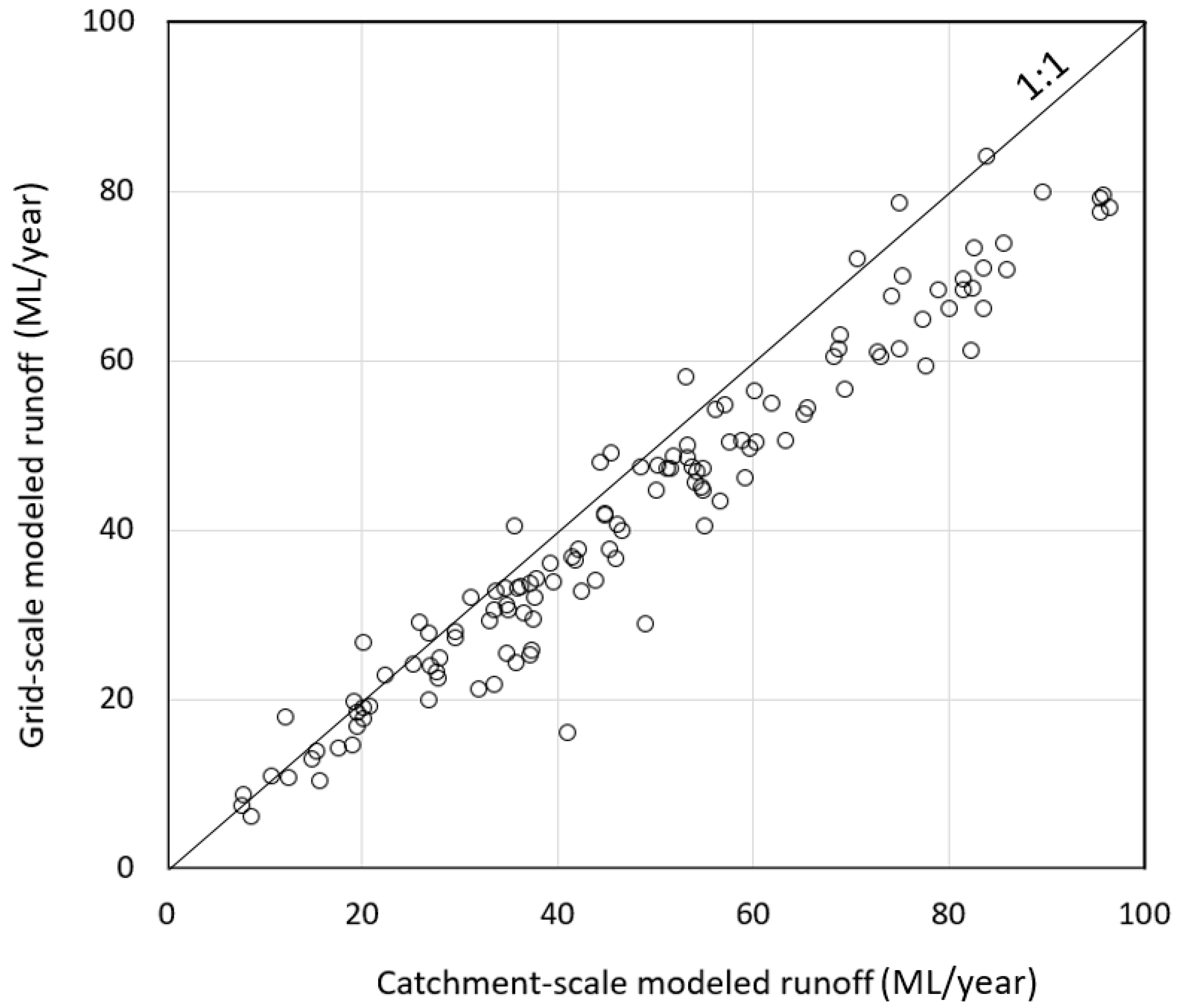
3.1. Comparison with the Catchment-Scale swTELR

Runoff outputs from the grid-based version of swTELR showed strong correspondence with the catchment-based model, with an R2 of 0.94 (Figure 3), which was expected, given that the two models share methods for curve number specification and runoff generation. The scale at which the calculations were performed was largely responsible for both the scatter in the relationship and a moderate negative bias (−13.7%) that reflected lower runoff predictions in the gridded version of the model. Most of this bias can be attributed to the large catchments located around the perimeter of Salinas with low impervious cover and a majority coverage of hydrologic soil group C, but with substantial proportions of more inflatable soils (groups A and B). While the catchment model assigned soil group C to the entire catchment, the grid model also represented the areas with more inflatable soils, resulting in less runoff production.

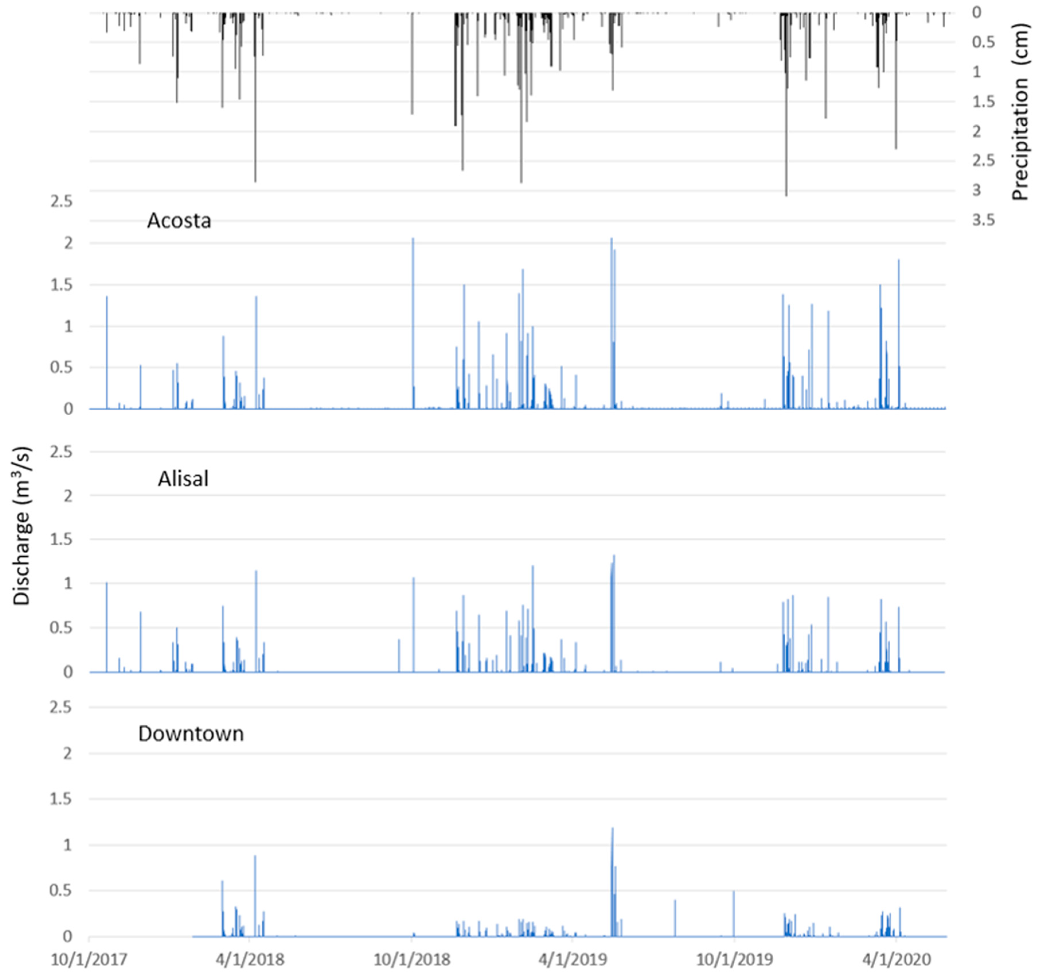
3.2. Flow Monitoring Data

Relative to the historical average annual rainfall in Salinas (37 cm), 2018 and 2020 water years (October–September) were dry, with 13.5 cm and 21.7 cm of rainfall, respectively, while 2019 was close to the average wetness (36.6 cm). Hydrographs for each catchment (Figure 4) over the course of the study period illustrate the similar runoff response for all three catchments, with the height of the peaks reflecting difference in drainage sizes. A summary of the monitoring data for each catchment in

Table 2. Outfall monitoring results’ summary for each water year.

			Acosta		Alisal		Downtown
Water Year	Number of Events > 1 cm	P (cm)	Q (ML/year)	Runoff Ratio	Q (ML/year)	Runoff Ratio	Q (ML/year)	RUNOFF RATIO
2018	38	18.5	76.5	0.30	64.1	0.36	29.8	0.22 *
2019	69	36.6	193.6	0.38	130.3	0.37	80.3	0.27
2020	42	21.7	156.3	0.52	106.0	0.51	55.6	0.34

* Adjusted for delayed installation of flow meter in water year 2018.

highlights differences in annual runoff response between the catchments, with Alisal showing the highest runoff ratio and with Downtown showing the lowest runoff ratio. The runoff ratios across years varied by 22%, 15%, and 12% in Acosta, Alisal, and Downtown, respectively. The consistently lower runoff ratios measured in the Downtown catchment were unexpected, since it has the highest degree of impervious cover with little disconnection of hard surfaces from the storm drain network.

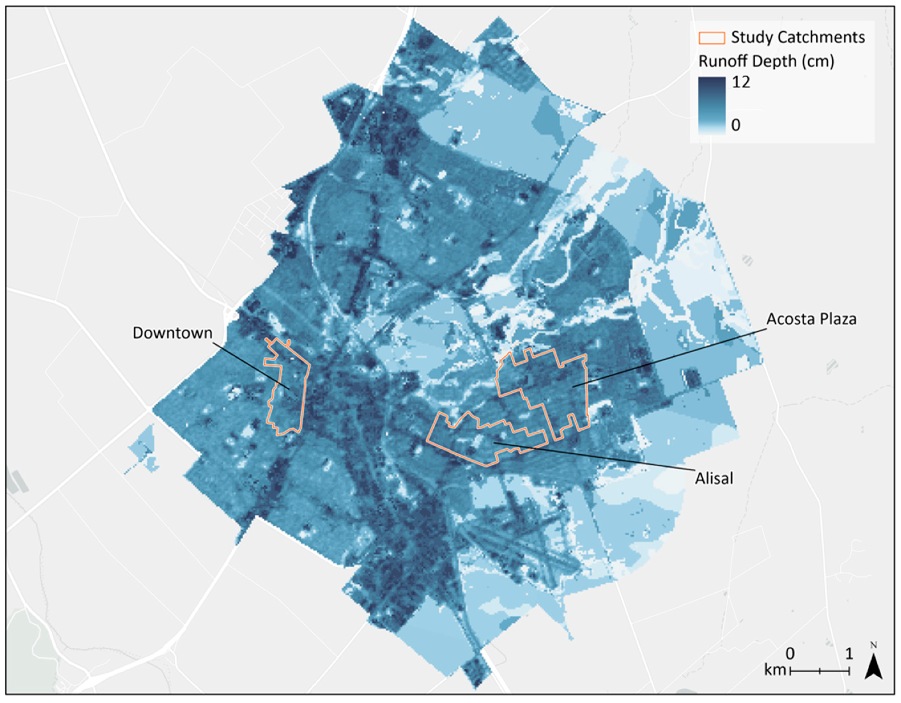
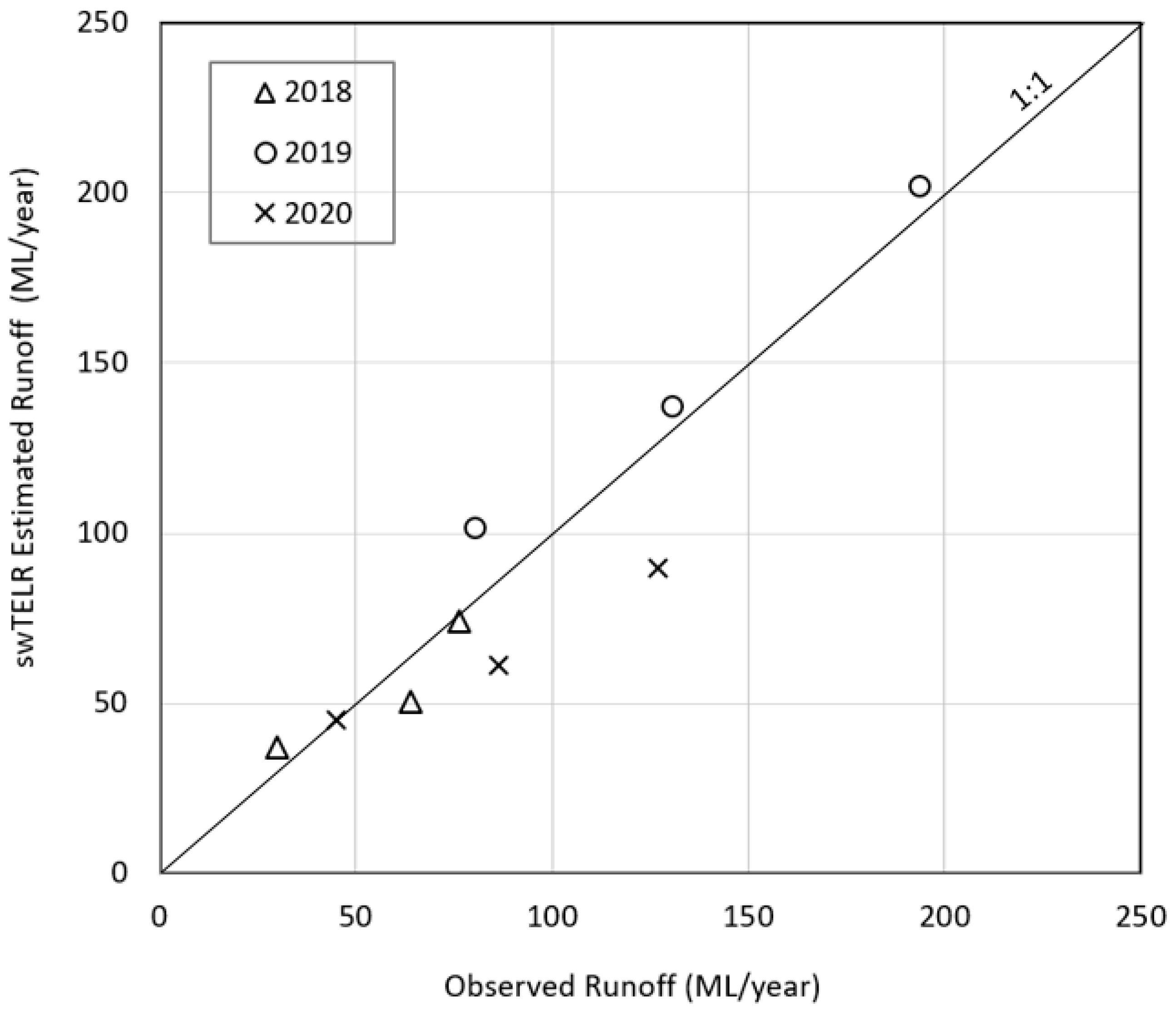
3.3. Runoff Estimates and Model Evaluation

Gridded outputs in Figure 5 shows the pattern of runoff generation throughout the city of Salinas for the water years 2017–2019, with the greatest runoff generation in areas with the highest impervious cover and the least inflatable soils (NRCS soil group D). With two very dry years included in this sequence, the average annual runoff depth over this period for all of Salinas was only 6.6 cm/year, corresponding to a runoff ratio of 0.26. As we would expect, areas with relatively high impervious cover, which correspond with the downtown, commercial, and industrial areas of the city, generally show higher annual runoff generation estimates, while large areas along the eastern outskirts of the city Municipal Separate Storm Sewer System (MS4) boundary, mostly occupied by cultivated crops and open space, have substantially lower runoff values compared to the area occupied by the study catchments. Thus, these model outputs provide a clear connection, at granular spatial scale, between the input data and runoff outputs that align with conceptual understanding of runoff generation drivers.

Correspondence between the modeled and observed annual runoff data is shown in Figure 6, with an R2 of 0.88 with a linear fit for all three catchments. While all catchments had at least one year with errors greater than 25% (see

Table 3. Comparison of observed and modeled annual runoff for each catchment. Negative errors indicate runoff under prediction by swTELR.

	Observed (ML/year)	swTELR (ML/year)	Error
		Acosta
2018	76.5	74	−3.3%
2019	193.6	202.1	4.4%
2020	127.1	89.8	−29.3%
		Alisal
2018	64.1	50.3	−21.5%
2019	130.3	137.5	5.5%
2020	86.8	61	−29.2%
		Downtown
2018	29.8	37	24.2%
2019	80.3	101.8	26.8%
2020	45.2	45	−0.4%
Totals	833.1	798.5	4.2%

), overall swTELR overestimated runoff by 4.2%. The largest errors were in 2020, with the model overestimating runoff by approximately 29% in both Alisal and Acosta. While the Downtown catchment performed worse than both Alisal and Acosta in 2018 and 2019, it showed the best performance in 2020 with an underestimate of only 0.4%. There was no consistent error pattern relative to annual rainfall totals, with over and under or over predictions occurring in both average and dry years for one or more of the catchments.

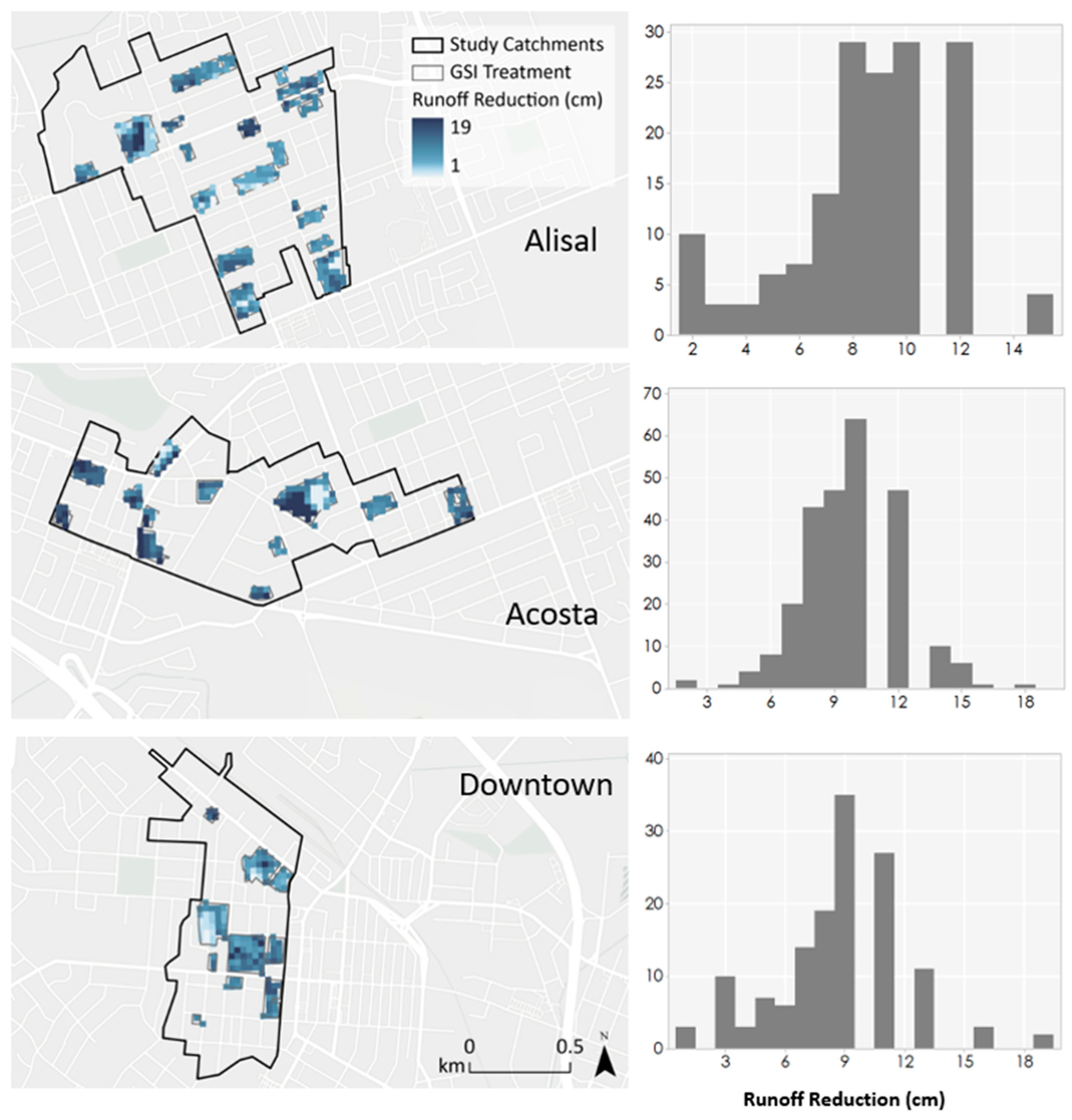
3.4. GSI Benefits Tracking

An example application of swTELR within the Salinas study catchments was completed to illustrate the utility of the model structure for tracking GSI runoff reductions over time. Parcels selected for implementation were delineated using a web browser-based geospatial application that stores these data for input to the swTELR GSI module (Figure 7). These parcels were clipped to the swTELR 30-m grid for calculating reductions associated with GSI treatment of the runoff generated within those areas. Since we wished to represent long-term runoff reductions, we used a rainfall sequence of 35 years (1981–2016) to drive runoff for these estimates, so that the baseline runoff available for infiltration was substantially greater than that shown in Figure 5. For this example, we assumed a design standard of 85th percentile storm depth capture for all BMPs, as is commonly specified in NPDES permits (e.g., California State Water Resources Control Board, 2013 [44]).

Examples of GSI implementation sites within the study catchments are shown in Figure 8, along with long-term annual runoff reductions. Even though a common design standard was applied for all sites, there was a range of annual runoff capture potential between 1–19 cm, depending on location, with differences primarily reflecting heterogeneity of soils and impervious cover. The mean annual runoff capture within potential implementation sites was 8–10 cm/year for all three catchments. These catchments are close together in the same city with flat terrain, so they use the same rainfall inputs, but cities or counties with large elevation or aspect changes within their NPDES permit boundaries would likely see greater variation in estimated runoff capture compared to these examples. Note that these estimates used a much longer rainfall time series (1981–2016) compared to that used in the baseline runoff validation experiments (2018–2020), since longer time series will tend to improve the precision of the percentile rainfall estimates. For example, when we ran the model using values from only those recent years to drive the model, since two of the three years were dryer than average, the result was less runoff production and less overall runoff infiltration, with a mean of 4.9–5.5 cm/year for all three catchments (results not shown). This is a substantially smaller annual runoff reduction than we would expect on average over the long-term lifespan of GSI features, which typically have design specifications dictated by long-term rainfall time series.

4. Discussion

4.1. Model Baseline Performance

While the modeled catchments showed good overall performance relative to the measured runoff data with little systematic bias in the outputs, individual catchments and years showed errors of up to 29%. Since performance adequacy thresholds have little meaning outside the context of the model use or a benchmark for comparison [45], the R2 value of 0.88 for the three catchments is difficult to interpret. One basis for comparison are simple empirical models, such as that used by Brezonik and Stadelmann (2002) [46], who found good performance for urban catchments in Minnesota, USA, achieving a maximum R2 value of 0.78. The swTELR provides a moderate improvement and above such estimates, but also may provide more reliable and transportable long-term estimates above regression model with coefficients that have been calibrated to a specific data set. Because the rainfall metrics were generated from individual rainfall years, this probably muted errors that would result from relying on the 35-year rainfall sequence that would normally drive swTELR baseline predictions and were used to estimate the GSI reductions. As additional catchment flow data are collected in subsequent years, they will provide a better basis for comparison of model outputs driven by long-term rainfall data. While errors are uncorrelated with the rainfall data, there does appear to be some correspondence between annual runoff ratios and model performance, with better model performance at higher runoff ratios. The exception to this rule was the Downtown catchment, which showed the best performance in 2020, with the lowest calculated runoff ratio observed (0.22).

Field investigations in the Downtown catchment during the end of a large storm in April 2019 uncovered evidence that some small areas mapped to the Downtown catchment outlet were actually routed to an adjacent, ungauged outlet. Also observed within the Downtown catchment were large areas of localized flooding caused by clogged storm drain inlets, which did not occur at other catchments. Both of these factors may have contributed to the over prediction of flows by swTELR in 2018 and 2019 and also relatively low measured runoff ratios that appear contradictory to the high impervious cover in this catchment. One explanation for the variable performance in all catchments from year to year is the lack of accounting for antecedent moisture conditions and the relevant dynamics in swTELR. For example, differences in rainfall characteristics during the three winters may have determined whether or not the observed storage differences from local flooding in the Downtown catchment affected the flow measured at the outlet. The flashy runoff response of these small, urbanized catchments is likely sensitive to the sequencing pattern of storms, which varies from year to year. Over longer periods, however, we would expect the relative stability of urban landscape characteristics, such as impervious cover, to be consistently influential drivers of runoff production. While a continuous simulation approach would provide an explicit accounting of rainfall patterns, the disadvantage is that spatial lumping or nonspatial methods typically used to characterize heterogeneity (e.g., Hydrologic Response Units [47]) may also reduce model utility for identifying parcel-scale GSI opportunities and benefits.

4.2. Application to GSI Tracking

Since there is no timing of flows included in the approach presented for tracking runoff reductions, it is only applicable to practices commonly associated with low impact development, where runoff is infiltrated close to where it is generated. The swTELR model handles larger, centralized treatment via a separate set of algorithms, which does incorporate flow timing based on drainage characteristics, which was reported by Beck et al. (2017) [31]. While the centralized treatment uses BMP design specifications to calculate infiltrated, treated, and bypassed flows explicitly, the GSI BMPs are assumed to infiltrate runoff up to their specified design storm. So, there is strong reliance on the assumption of adherence to BMP sizing standards. Given that there may be hundreds or thousands of GSI BMPs distributed throughout a city, these simplifications allow computation entirely with raster-based algorithms, so that it is fast enough to be run via a web browser, allowing users to run various heuristic implementation scenarios.

Probabilistic treatment of the rainfall inputs in swTELR simplifies computation in favor of spatially explicit representation of GSI locations. Consequently, swTELR model outputs depend more strongly on inputs such as impervious cover, which can be reliably measured from imagery, rather than parameter values derived from fitting observed flows. While such fitting can provide more accurate short-term predictions, parameter estimates are often difficult to associate with physical catchment characteristics and typically unverifiable at meaningful spatial scales [48,49]. Since there is often no hydrologic data available to characterize urban drainages, stormwater planning model applications often rely on much larger drainage areas with relatively little urban coverage for calibration or regionalization of parameters from neighboring watersheds (e.g., San Mateo Countywide Water Pollution Prevention Program, 2018 [50]). Simpler process representation avoids tying model outputs to short time periods for calibration, which may create strong dependence on those calibration data [51] or areas with runoff responses largely driven by non-urban areas. It also facilitates better use of geographic and remotely sensed data, previously called for in a review of GSI models by Jayasooriya and Ng (2014) [32], allowing for spatially explicit characterization of site-level conditions, which may play a critical role in GSI benefits calculations [17], as illustrated by swTELR outputs in Figure 8. The approach presented also allows specification of individual BMP performance condition changes over time, which can be field verified and can be a key factor in overall GSI performance [52,53,54,55].

Given the coarse time resolution employed by swTELR, estimated changes over time will rely on aggregate measures, such as runoff ratios and annual runoff volumes, rather than individual hydrograph characteristics such as peak flow height or time to peak. Matching runoff changes associated with GSI implementation will likely be more difficult than matching baseline flows since such changes will need to be outside the envelope of model error and also will need to be detectable above the natural hydrologic variation in the catchment runoff. Another confounding factor is that GSI is most effective at mitigating lower intensity events [56] and may have a more muted effect on the larger events that drive much of the aggregate runoff volume response. Such detection of changes will probably be limited to relatively small catchments with intensive GSI implementation. In the Salinas study catchments, currently planned implementation will treat up to 40% of the impervious surface coverage with GSI by 2030. Such an intensive GSI campaign may indeed produce measurable hydrologic changes in the aggregate hydrologic metrics that align with the swTELR outputs. This would provide a practical method for scaling GSI reduction estimates as outlined by Golden and Hoghooghi (2018) [18], who highlighted the need to address the challenge of aggregating fine-scale process heterogeneity up to catchment scales for meaningful demonstration of GSI effectiveness. As monitoring continues at the Salinas study catchments, and GSI implementation proceeds, future work will include analysis to detect changes in the hydrologic time series and ongoing comparisons with the model estimates.

Modeling tools that are more dynamic and directly verifiable can better serve the evolving needs of stormwater managers. As priorities, opportunities, and technology shift over time, models that can incorporate new information as it becomes available and provide outputs on timeframes and spatial scales that match those of decision making are more useful for prioritization and long-term tracking. There is a risk that the trade-offs chosen to optimize a model structure for these purposes compromise the accuracy of outputs to an unacceptable degree, but this risk can be minimized by collecting monitoring data at the appropriate scale, as we have demonstrated in Salinas. Long-term urban catchment monitoring provides a mechanism for interim verification of model inputs and assumptions to help build the technical foundation for transparent quantification of expected GSI hydrologic benefits. A transparent stormwater accounting system is a key technical gap for newly emerging stormwater program funding structures, such as public private partnerships, that can help to accelerate the pace of GSI implementation for cities but require science-based means for demonstrating progress toward milestones. When paired with asset management systems to track the locations, types, and condition of GSI features, outputs from models such as swTELR can provide stormwater managers with a dynamic source of information from which to make decisions regarding new implementation, maintenance, and program effectiveness.

5. Conclusions

We introduced a novel method for tracking the runoff reduction benefits of GSI with a design optimized to the meet the needs of stormwater managers that uses probabilistic rainfall inputs, raster-based cloud computation, and web-based tools for delineating individual drainages. Where the previous version of swTELR lumped attributes at the catchment scale (40 ha) to estimate centralized stormwater treatment benefits, this version provides a spatially explicit accounting of GSI at the sub-parcel level. Baseline runoff estimates correspond with outputs from the previous catchment-based version of the model, but the inputs and outputs of the current version align much better with the spatial scale of GSI planning and implementation. The revised structure allows sequencing of runoff reductions with user-defined GSI drainages nested within centralized treatment drainages to ensure internal consistency of calculated runoff reductions. Municipal users access the model via a web portal that allows them to enter GSI projects, delineate BMP drainages, verify BMP performance, and generate updated estimates of runoff reductions associated with both GSI and centralized runoff treatment.

Baseline runoff verification experiments within the City of Salinas, CA, USA, showed very good overall correspondence between swTELR and measured annual flows, with large errors in one of the catchments at least partially attributable to inaccurate catchment delineation and storm drain network failure. The model shows good potential as a tracking and decision support tool, particularly when preserving site-specific attributes for GSI runoff reduction estimates and input data updatability is important, such as for ongoing municipal NPDES permit reporting. A critical trade-off for the detailed spatial representation and wide coverage of runoff reduction estimates is the lack of ability to simulate changes in individual storm hydrographs that may be attributable to GSI implementation. The Salinas examples illustrate how planned parcel-level GSI reductions can be efficiently scaled up to urban catchments and provide outputs that are amenable to catchment-scale verification, shortening the information feedback interval from modeling to monitoring. As GSI implementation proceeds, the Salinas study catchments should provide a strong basis for detecting aggregate catchment-scale hydrologic changes and also provide an opportunity for comparison with modeled runoff reductions.

6. Patents

Systems and Methods for Event-based Modeling of Runoff and Pollutant Benefits of Sustainable Stormwater Management. U.S. Patent No.10,754,061; Issue date 25 August 2020.

References

1. Booth, D.B.; Jackson, C.R. Urbanization of aquatic systems: Degradation thresholds, stormwater detection, and the limits of mitigation. JAWRA J. Am. Water Resour. Assoc. 1997, 33, 1077–1090. [Google Scholar] [CrossRef]
2. Tang, Z.; Engel, B.; Pijanowski, B.; Lim, K. Forecasting land use change and its environmental impact at a watershed scale. J. Environ. Manag. 2005, 76, 35–45. [Google Scholar] [CrossRef] [PubMed]
3. US EPA (Environmental Protection Agency). Our Built and Natural Environments: A Technical Review of the Interactions between Land Use, Transportation, and Environmental Quality, 2nd ed.; EPA 231-K-13-001; US EPA: Washington, DC, USA, 2013.
4. Pennino, M.J.; McDonald, R.I.; Jaffe, P.R. Watershed-scale impacts of stormwater green infrastructure on hydrology, nutrient fluxes, and combined sewer overflows in the mid-Atlantic region. Sci. Total Environ. 2016, 565, 1044–1053. [Google Scholar] [CrossRef] [PubMed] [Green Version]
5. Davis, A.P. Field Performance of Bioretention: Water Quality. Environ. Eng. Sci. 2007, 24, 1048–1064. [Google Scholar] [CrossRef]
6. Venkataramanan, V.; Lopez, D.; McCuskey, D.J.; Kiefus, D.; McDonald, R.I.; Miller, W.M.; Packman, A.I.; Young, S.L. Knowledge, attitudes, intentions, and behavior related to green infrastructure for flood management: A systematic literature review. Sci. Total Environ. 2020, 720, 137606. [Google Scholar] [CrossRef]
7. Tao, J.; Li, Z.; Peng, X.; Ying, G. Quantitative analysis of impact of green stormwater infrastructures on combined sewer overflow control and urban flooding control. Front. Environ. Sci. Eng. 2017, 11, 11. [Google Scholar] [CrossRef]
8. Zellner, M.L.; Massey, D.; Minor, E.; Gonzàlez-Meler, M.A. Exploring the effects of green infrastructure placement on neighborhood-level flooding via spatially explicit simulations. Comput. Environ. Urban. Syst. 2016, 59, 116–128. [Google Scholar] [CrossRef] [Green Version]
9. Dussaillant, A.R.; Cuevas, A.; Potter, K.W. Raingardens for stormwater infiltration and focused groundwater re-charge: Simulations for different world climates. Water Sci. Technol. Water Supply 2005, 5, 173–179. [Google Scholar] [CrossRef]
10. Bhaskar, A.S.; Hogan, D.M.; Nimmo, J.R.; Perkins, K.S. Groundwater recharge amidst focused stormwater infiltration. Hydrol. Process. 2018, 32, 2058–2068. [Google Scholar] [CrossRef]
11. Chen, W.Y. The role of urban green infrastructure in offsetting carbon emissions in 35 major Chinese cities: A nationwide estimate. Cities 2015, 44, 112–120. [Google Scholar] [CrossRef]
12. Foster, J.; Lowe, A.; Winkelman, S. The value of green infrastructure for urban climate adaptation. Cent. Clean Air Policy 2011, 750, 1–52. [Google Scholar]
13. Gill, S.E.; Handley, J.F.; Ennos, A.R.; Pauleit, S. Adapting cities for climate change: The role of the green infra-structure. Built Environ. 2007, 33, 115–133. [Google Scholar] [CrossRef] [Green Version]
14. Clary, J.; Urbonas, B.; Jones, J.; Strecker, E.; Quigley, M.; O’Brien, J. Developing, evaluating and maintaining a standardized stormwater BMP effectiveness database. Water Sci. Technol. 2002, 45, 65–73. [Google Scholar] [CrossRef] [PubMed]
15. Strecker, E.W.; Quigley, M.M.; Urbonas, B.; Jones, J. Analyses of the Expanded EPA/ASCE International BMP Database and Potential Implications for BMP Design. Crit. Transit. Water Environ. Resour. Manag. 2004, 1–10. [Google Scholar] [CrossRef]
16. Ackerman, D.; Stein, E.D. Evaluating the Effectiveness of Best Management Practices Using Dynamic Modeling. J. Environ. Eng. 2008, 134, 628–639. [Google Scholar] [CrossRef]
17. Jarden, K.M.; Jefferson, A.J.; Grieser, J.M. Assessing the effects of catchment-scale urban green infrastructure retrofits on hydrograph characteristics. Hydrol. Process. 2016, 30, 1536–1550. [Google Scholar] [CrossRef]
18. Golden, H.E.; Hoghooghi, N. Green infrastructure and its catchment-scale effects: An emerging science. Wiley Interdiscip. Rev. Water 2018, 5, e1254. [Google Scholar] [CrossRef] [PubMed] [Green Version]
19. Ahiablame, L.M.; Engel, B.A.; Chaubey, I. Effectiveness of low impact development practices in two urbanized water-sheds: Retrofitting with rain barrel/cistern and porous pavement. J. Environ. Manag. 2013, 119, 151–161. [Google Scholar] [CrossRef]
20. Loperfido, J.; Noe, G.B.; Jarnagin, S.T.; Hogan, D.M. Effects of distributed and centralized stormwater best management practices and land cover on urban stream hydrology at the catchment scale. J. Hydrol. 2014, 519, 2584–2595. [Google Scholar] [CrossRef]
21. Kong, F.; Ban, Y.; Yin, H.; James, P.; Dronova, I. Modeling stormwater management at the city district level in response to changes in land use and low impact development. Environ. Model. Softw. 2017, 95, 132–142. [Google Scholar] [CrossRef]
22. Avellaneda, P.M.; Jefferson, A.J.; Grieser, J.M.; Bush, S.A. Simulation of the cumulative hydrological response to green infrastructure. Water Resour Res. 2017, 53, 3087–3101. [Google Scholar] [CrossRef]
23. Vogel, J.R.; Moore, T.L.; Coffman, R.R.; Rodie, S.N.; Hutchinson, S.L.; McDonough, K.R.; McLemore, A.J.; McMaine, J.T. Critical Review of Technical Questions Facing Low Impact Development and Green Infrastructure: A Perspective from the Great Plains. Water Environ. Res. 2015, 87, 849–862. [Google Scholar] [CrossRef] [PubMed]
24. Sarkar, S.; Butcher, J.B.; Johnson, T.E.; Clark, C.M. Simulated Sensitivity of Urban Green Infrastructure Practices to Climate Change. Earth Interact. 2018, 22, 1–37. [Google Scholar] [CrossRef] [PubMed]
25. Roy, A.H.; Rhea, L.K.; Mayer, A.L.; Shuster, W.D.; Beaulieu, J.J.; Hopton, M.E.; Morrison, M.A.; Amand, A.S. How Much Is Enough? Minimal Responses of Water Quality and Stream Biota to Partial Retrofit Stormwater Management in a Suburban Neighborhood. PLoS ONE 2014, 9, e85011. [Google Scholar] [CrossRef] [PubMed]
26. California State Water Resources Control Board (CA SWRCB). Municipal Regional Stormwater Permit for the San Francisco Bay Region; Order Number R2-2015-0049; San Francisco Bay Regional Water Quality Control Board: Oakland, CA, USA, 2015; p. 359.
27. Petrucci, G.C.; Bonhomme, R. The dilemma of spatial representation for urban hydrology semi-distributed modelling: Trade-offs among complexity, calibration, and geographical data. J. Hydrol. 2014, 517, 997–1007. [Google Scholar] [CrossRef]
28. Yuan, L.; Sinshaw, T.; Forshay, K.J. Review of Watershed-Scale Water Quality and Nonpoint Source Pollution Models. Geosciences 2020, 10, 25. [Google Scholar] [CrossRef] [Green Version]
29. Kokkonen, T.S.; Jakeman, A.J. A comparison of metric and conceptual approaches in rainfall-runoff modeling and its implications. Water Resour. Res. 2001, 37, 2345–2352. [Google Scholar] [CrossRef] [Green Version]
30. Dotto, C.B.S.; Kleidorfer, M.; Deletic, A.; Rauch, W.; McCarthy, D.; Fletcher, T. Performance and sensitivity analysis of stormwater models using a Bayesian approach and long-term high resolution data. Environ. Model. Softw. 2011, 26, 1225–1239. [Google Scholar] [CrossRef]
31. Beck, N.G.; Conley, G.; Kanner, L.; Mathias, M. An urban runoff model designed to inform stormwater management decisions. J. Environ. Manag. 2017, 193, 257–269. [Google Scholar] [CrossRef]
32. Jayasooriya, V.M.; Ng, A.W.M. Tools for modeling of stormwater management and economics of green infra-structure practices: A review. WaterAirSoil Pollut. 2014, 225, 2055. [Google Scholar] [CrossRef] [Green Version]
33. USDA-NRCS (U.S. Department of Agriculture-Natural Resources Conservation Service). Urban Hydrology for Small Watersheds, 2nd ed.; Technical Release 55; NTIS PB87-101580; USDA NRCS: Springfield, VA, USA, 1986.
34. Woodward, D.E.; Hawkins, R.H.; Jiang, R.; Hjelmfelt, A.T., Jr.; Van Mullem, J.A.; Quan, Q.D. Runoff curve number method: Examination of the initial abstraction ratio. World Water Environ. Resour. Congr. 2003, 1, e10. [Google Scholar] [CrossRef] [Green Version]
35. Lim, K.J.; Engel, B.; Muthukrishnan, S.; Harbor, J.; Harbor, J. Effects of initial abstraction and urbanization on estimated runoff using Cn technology. JAWRA J. Am. Water Resour. Assoc. 2006, 42, 629–643. [Google Scholar] [CrossRef]
36. Michel, C.; Andréassian, V.; Perrin, C. Soil Conservation Service Curve Number method: How to mend a wrong soil moisture accounting procedure? Water Resour. Res. 2005, 41, 17. [Google Scholar] [CrossRef]
37. Jiang, R. Investigation of Runoff Curve Number Initial Abstraction Ratio. Master’s Thesis, University of Arizona, Tucson, AZ, USA, 2001. Available online: http://arizona.openrepository.com/arizona/handle/10150/191301 (accessed on 10 September 2015).
38. Hawkins, R.H.; Jiang, R.; Woodward, D.E.; Hjelmfelt, A.T.; Van Mullem, J.A. Runoff Curve Number Method: Examination of the Initial Abstraction Ratio. In Proceedings of the Second Federal Interagency Hydrologic Modeling Conference, Las Vegas, NV, USA, 28 July–1 August 2002; U.S. Geological Survey: Lakewood, CO, USA. [Google Scholar]
39. PRISM Climate Group. Oregon State University. Available online: http://prism.oregonstate.edu (accessed on 4 February 2004).
40. R Core Team. R: A Language and Environment for Statistical Computing; R Foundation for Statistical Computing: Vienna, Austria, 2018; Available online: https://www.R-project.org/ (accessed on 10 November 2020).
41. Hijmans, R.J. Raster: Geographic Data Analysis and Modeling. Available online: https://CRAN.R-project.org/package=raster (accessed on 15 August 2017).
42. National Land Cover Database (NLCD). Urban Imperviousness, Updated 2016. Available online: https://www.mrlc.gov/ (accessed on 1 October 2017).
43. Manning, R.; Griffith, J.P.; Pigot, T.F.; Vernon-Harcourt, L.F. On the flow of water in open channels and pipes. Trans. Inst. Civ. Eng. Irel. 1890, 20, 161–207. [Google Scholar]
44. California State Water Resources Control Board (CCRWQCB). Stormwater Discharges from Small Municipal Separate Storm Sewer Systems; Water Quality Order No. 2013-0001-DWQ; General Permit No. CAS000004; California State Water Resources Control Board: Oakland, CA, USA, 2013.
45. Schaefli, B.; Gupta, H.V. Do Nash values have value? Hydrol. Process. 2007, 21, e2075–e2080. [Google Scholar] [CrossRef] [Green Version]
46. Brezonik, P.L.; Stadelmann, T.H. Analysis and predictive models of stormwater runoff volumes, loads, and pollutant concentrations from watersheds in the Twin Cities metropolitan area, Minnesota, USA. Water Res. 2002, 36, 1743–1757. [Google Scholar] [CrossRef]
47. Leavesly, G.H.; Lichty, R.W.; Troutman, B.M.; Saindon, L.G. Precipitaion and Runoff Modelling System—User’s Manual; USGS Water Resources Investigation Report 83—4238; US Department of the Interior: Washington, DC, USA, 1983.
48. Beven, K.J. Prophecy, reality and uncertainty in distributed hydrological modelling. Adv. Water Resour. 1993, 16, 41–51. [Google Scholar] [CrossRef]
49. Beven, K. A manifesto for the equifinality thesis. J. Hydrol. 2006, 320, 18–36. [Google Scholar] [CrossRef] [Green Version]
50. San Mateo County Water Pollution Prevention Program (SMCWPPP). Phase I Baseline Modeling Report—Provides Documentation of the Development, Calibration, and Validation of the Baseline Hydrology and Water Quality Model, and the Determination of PCB and Mercury Load Reductions to be Addressed through GI Implementation; Final Report; San Mateo Countywide Pollution Prevention Program: Redwood City, CA, USA, 2018; p. 169.
51. Bertrand-Krajewski, J.-L. Stormwater pollutant loads modelling: Epistemological aspects and case studies on the influence of field data sets on calibration and verification. Water Sci. Technol. 2007, 55, 1–17. [Google Scholar] [CrossRef]
52. Siriwardene, N.R.; Deletic, A.; Fletcher, T.D. Preliminary studies of the development of a clogging prediction meth-od for stormwater infiltration systems. Water Pract. Technol. 2007, 2, 1–8. [Google Scholar] [CrossRef]
53. Kandra, H.S.; McCarthy, D.; Fletcher, T.D.; Deletic, A. Assessment of clogging phenomena in granular filter media used for stormwater treatment. J. Hydrol. 2014, 512, 518–527. [Google Scholar] [CrossRef] [Green Version]
54. Tu, M.-C.; Traver, R.G. Clogging Impacts on Distribution Pipe Delivery of Street Runoff to an Infiltration Bed. Water 2018, 10, 1045. [Google Scholar] [CrossRef] [Green Version]
55. Conley, G.; Beck, N.; Riihimaki, C.A.; Tanner, M. Quantifying clogging patterns of infiltration systems to im-prove urban stormwater pollution reduction estimates. Water Res. X 2020. [Google Scholar] [CrossRef] [PubMed]
56. Giese, E.; Rockler, A.; Shirmohammadi, A.; Pavao-Zuckerman, M.A. Assessing Watershed-Scale Stormwater Green Infrastructure Response to Climate Change in Clarksburg, Maryland. J. Water Resour. Plan. Manag. 2019, 145, 05019015. [Google Scholar] [CrossRef]
Figure 1. Structural overview for the grid based swTELR model with raster processing workflow. Green Stormwater Infrastructure (GSI) elements are described in this study and centralized treatment algorithms were reported in Beck et al., 2017 [31].
Water 13 00255 g001
Figure 2. Study catchment locations and attributes within the City of Salinas, CA, USA.
Water 13 00255 g002
Figure 3. Comparison between grid-scale and catchment-scale runoff estimates from swTELR for all Salinas catchments (n = 131).
Water 13 00255 g003
Figure 4. Rainfall and flow data collected at catchment outfalls during water years 2018–2020. Note that instrumentation was delayed in the Downtown catchment until January 2018.
Water 13 00255 g004
Figure 5. The swTELR average annual runoff depth estimates for City of Salinas for water years 2018–2020.
Water 13 00255 g005
Figure 6. The swTELR annual runoff estimates compared to observed flows for the three study catchments.
Water 13 00255 g006
Figure 7. Web-based Green Stormwater Infrastructure (GSI) site delineation tool used in swTELR.
Water 13 00255 g007
Figure 8. Estimated long-term annual runoff reductions from swTELR for potential Green Stormwater Infrastructure (GSI)implementation sites in Salinas. Histograms show grid cell counts in each study catchment.
Water 13 00255 g008