
Improving Flow Discharge-Suspended Sediment Relations: Intelligent Algorithms versus Data Separation


1
Department of Watershed Management Engineering, Sari Agricultural Sciences and Natural Resources University, Sari 4818168984, Iran
2
Faculty of Natural Resources and Environment, Ferdowsi University of Mashhad, Mashhad 9177948974, Iran
3
Mountain Societies Research Institute, University of Central Asia, Khorog 736000, Tajikistan
*
Author to whom correspondence should be addressed.
Water 2021, 13(24), 3650; https://doi.org/10.3390/w13243650
Submission received: 23 November 2021
/
Revised: 12 December 2021
/
Accepted: 16 December 2021
/
Published: 19 December 2021
(This article belongs to the Special Issue Extreme Hydrology: Induced Impacts and Vulnerability of Water Resources)
Abstract
:Information on the transport of fluvial suspended sediment loads (SSL) is crucial due to its effects on water quality, pollutant transport and transformation, dam operations, and reservoir capacity. As such, adopting a reliable method to accurately estimate SSL is a key topic for watershed managers, hydrologists, river engineers, and hydraulic engineers. One of the most common methods for estimating SSL or suspended sediment concentrations (SSC) is sediment rating curve (SRC), which has several weaknesses. Here, we optimize the SRC equation using two main approaches. Firstly, three well recognized metaheuristic algorithms (genetic algorithm (GA), particle swarm optimization (PSO), and imperialist competitive algorithm (ICA)) were used together with two classical approaches (food and agriculture organization (FAO) and non-parametric smearing estimator (CF2)) to optimize the coefficients of the SRC regression model. The second approach uses separation of data based on season and flow discharge (Qw) characteristics. A support vector regression (SVR) model using only Qw as an input was employed for SSC estimation and the results were compared with the SRC and its optimized versions. Metaheuristic algorithms improved the performance of the SRC model and the PSO model outperformed the other algorithms. These results also indicate that the model performance was directly related to the temporal separation of data. Based on these findings, if data are more homogenous and related to the limited climatic conditions used in the estimation of SSC, the estimations are improved. Moreover, it was observed that optimizing SRC through metaheuristic models was much more effective than separating data in the SCR model. The results also indicated that with the same input data, SVR was superior to the SRC model and its optimized version.
1. Introduction
Having adequate up-to-date information about sediment loads in rivers is important for hydraulic, river engineering, and water resources projects [1,2]. Sediment transport changes channel dynamics and ecologic and hydraulic conditions of the river [3]. Following the definitions of Einstein [4], a river can carry sediment in two distinct modes: bed load and suspended load that depend on particle size, weight and shape, and on the ambient hydraulic conditions. The fluvial sediment load is commonly measured directly or calculated indirectly [3]. Typically, due to lack of facilities, technical constraints, difficulty in accessing remote areas, and high costs, direct and continuous collection of sediment data is not possible, especially in developing countries like Iran [5]. A review of previous studies shows that, many researchers used indirect methods or alternative approaches for estimating of bed load [6,7,8,9] and suspended load [6,10]. Most of these sediment transport functions require comprehensive information on the channel, flow conditions, and sediment characteristics [11]. Therefore, use of simple methods with accessible parameters to estimate sediment load is a more practical alternative; such relationships can be derived using regression analysis [3]. Sediment rating curve (SRC) is the most common regression-based model which has been applied throughout the world in different environmental conditions to estimate suspended sediment in rivers [12,13,14,15,16,17,18,19,20]. This method expresses the empirical relationship between suspended sediment loads (SSL) or suspended sediment concentrations (SSC) and flow discharge (Qw) by power, linear, or polynomial functions [13,19,20,21,22,23].
However, there are several weaknesses with the SRC that generate inaccuracies in modeling and estimation of SSL. The first limitation arises from the bias caused by the logarithmic transformation of data during the computation of model coefficients, which leads to underestimation [13,24]. The second limitation is associated with the extrapolation of sediment values at high discharge [25]. Because most of the values used in construction of the SRC are at low flows, the majority of the suspended load in rivers and streams occurs during flood periods. This generally leads to higher error in suspended load estimation at high discharge [12,26]. The third limitation is the typical wide scatter of values around the regression line with long-term suspended sediment against discharge data [13]. This can arise because, in the SRC model, suspended sediment is estimated based on discharge, while the amount of suspended sediment at equal discharge values may be variable in different events (e.g., rainfall, snowmelt, base flow [27]. This can also be seen in the event of flood hydrograph, where the amount of suspended sediment at a constant discharge, in the beginning of the rising limb of the hydrograph, can be quite different from that in the falling limb (i.e., hysteresis effects [28]). This is because, while a large amount of sediment is usually available for transport on the rising limb and peak flow, on the falling limb, less sediment is available for transport; however, in some cases, this hysteresis can be reversed [26]. In addition, the occurrence of successive floods reduces the sediment load in a river, which may result in different amounts of sediment load at equal discharges [29,30].
To overcome these limitations with SRC’s, various methods have been suggested. Among these are classical correction coefficient models such as the food and agriculture organization (FAO), quasi-maximum likelihood estimator (QMLE), and non-parametric smearing estimator (CF2) [24,31,32]. Despite their differences, the common aim of these models is to increase the accuracy of calculated values by SRC. Another way of tackling this problem is to prepare different SRC models based on time separation of data (e.g., seasons, months) and based on flow characteristics (e.g., high water and low water periods, similar hydrological periods, discharge classes). Various studies have confirmed that classification of data into hydrological groups and increasing time resolution can lead to better model performance [16,17,19,26,33,34,35,36,37,38,39,40]. In fact, the goal of data separation is to reduce data scatter around the regression line and increase the estimation power of the model.
Alternatively, to increase the accuracy of SSL estimation, the use of intelligent algorithms as a type of nonlinear network has recently revolutionized forecasts and estimates of suspended sediment in rivers worldwide [41,42,43,44,45,46,47,48]. Metaheuristic algorithms are considered as one of the most important types of intelligent algorithms for optimization problems in a within wide spectrum of applications. These algorithms randomly search for optimal solutions in the problem-solving space, but purposefully [49], and perform well in solving various optimization problems, such as nonlinear, non-convex, or noisy functions [50]. The application of different types of metaheuristic optimization algorithms to water resources projects has been increasing in recent years [51,52,53,54,55,56]. To optimize SRC coefficients using metaheuristic algorithms, Tabatabaei et al. [57] compared genetic algorithm (GA) and non-dominated sorting genetic algorithm II (NSGA-II) with traditional methods, namely FAO, QMLE, and Smearing. Their results indicated the superiority of NSGA-II over the other methods. Tabatabaei and Salehpour Jam [58] used GA and particle swarm optimization (PSO) algorithms; Pour et al. [59] used GA and ant colony optimization (ACO) algorithms; Ebrahimi et al. [60] used GA and honey-bees mating optimization (HBMO) algorithm; Altunkaynak [61] used GA to optimize SRC; all of these studies observed high efficiency using these algorithms. Furthermore, the algorithms of teaching–learning based optimization (TLBO) and artificial bee colony (ABC) were employed to optimize the coefficients in regression equations for estimating SSL. Results indicated that ABC and TLBO algorithms were more efficient than traditional methods [62].
Considering the global use of the SRC method among experts and researchers, as well as its limitations, our study focuses on finding the most effective methods for improving such applications. As such, our study aims to improve the flow discharge–suspended sediment relation by: (1) optimizing the coefficients of SRC using metaheuristic algorithms such as imperialist competitive algorithm (ICA), PSO, and GA and classic corrective methods (FAO and CF2); (2) improving the SRC-based on time separation of data (seasonal) and flow characteristics; and (3) developing a support vector regression (SVR) model using only Qw as an input to provide similar conditions to those in the SRC method. Besides, when developing intelligent models, the main emphasis is often on the optimum design of intelligent networks and determination of the type of input data, whereas the separation of input data has rarely been considered. Therefore, in our study, a comprehensive comparison of different SSC estimation models is conducted to accurately determine the most effective methods.
2. Study Area and Database
2.1. Study Area
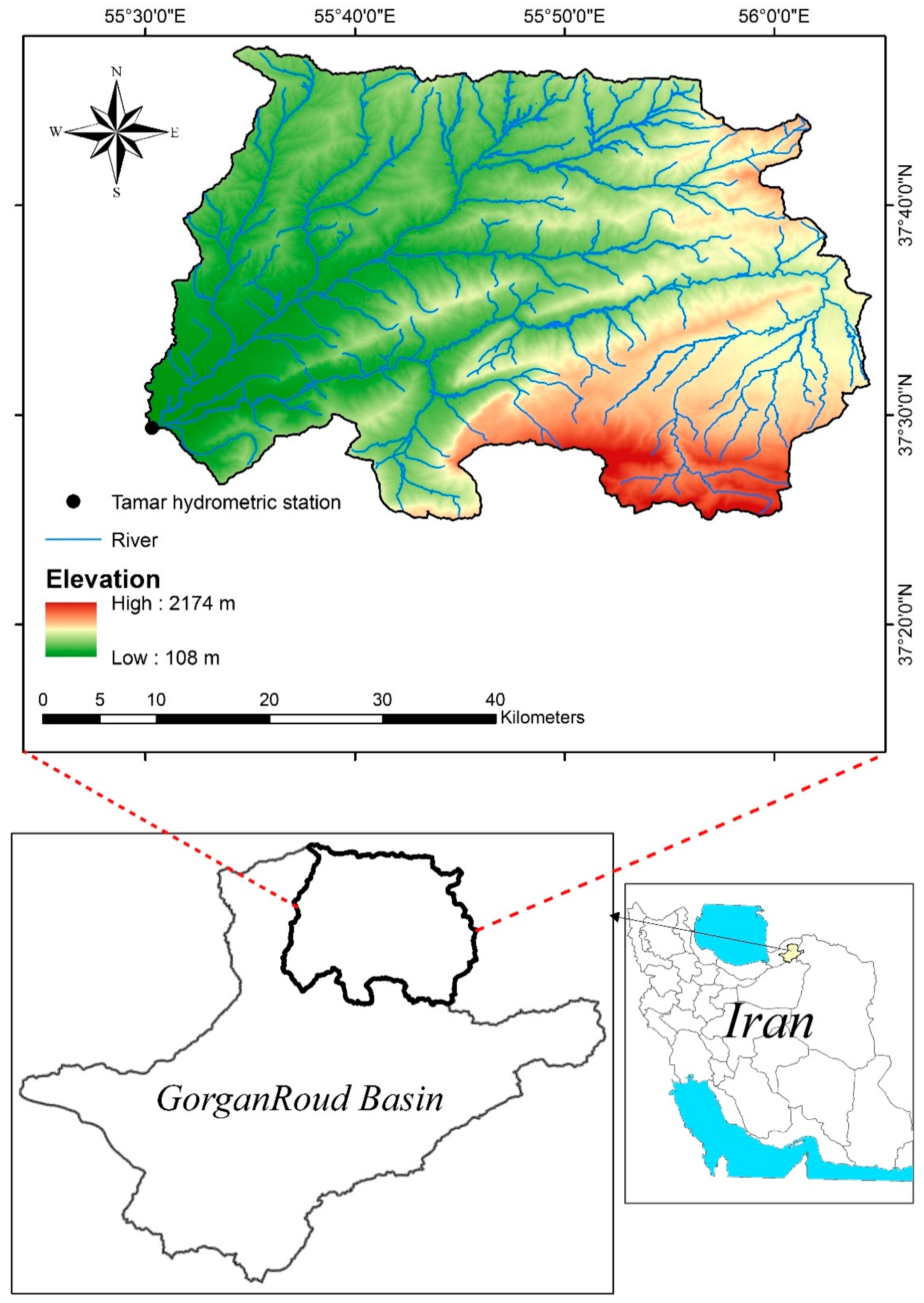
Boostan dam watershed with an area of 1533.3 km2 located between 37° 24′ 05″ and 37° 47′ 33″ North latitude and 54° 29′ 30″ and 56° 05′ 35″ East longitude is a sub-basin of GorganRoud basin. Golestan province, Iran (Figure 1). This watershed was selected as a case study due to the availability of data and the absence of major abstractions or dams in the upstream reaches. Boostan dam watershed has an elevation range from 108 to 2174 m a.s.l. (mean = 753 m) and an average slope gradient of 23%. According to the Amberje climate classification, the regional climate types include moderate semi-humid, cold humid, cold arid, and moderate semi-arid in different parts of the watershed. Average annual precipitation, average annual temperature, and relative humidity of the region are 483 mm, 17.8 °C, and 68.5%, respectively.
2.2. Data and Data Preprocessing
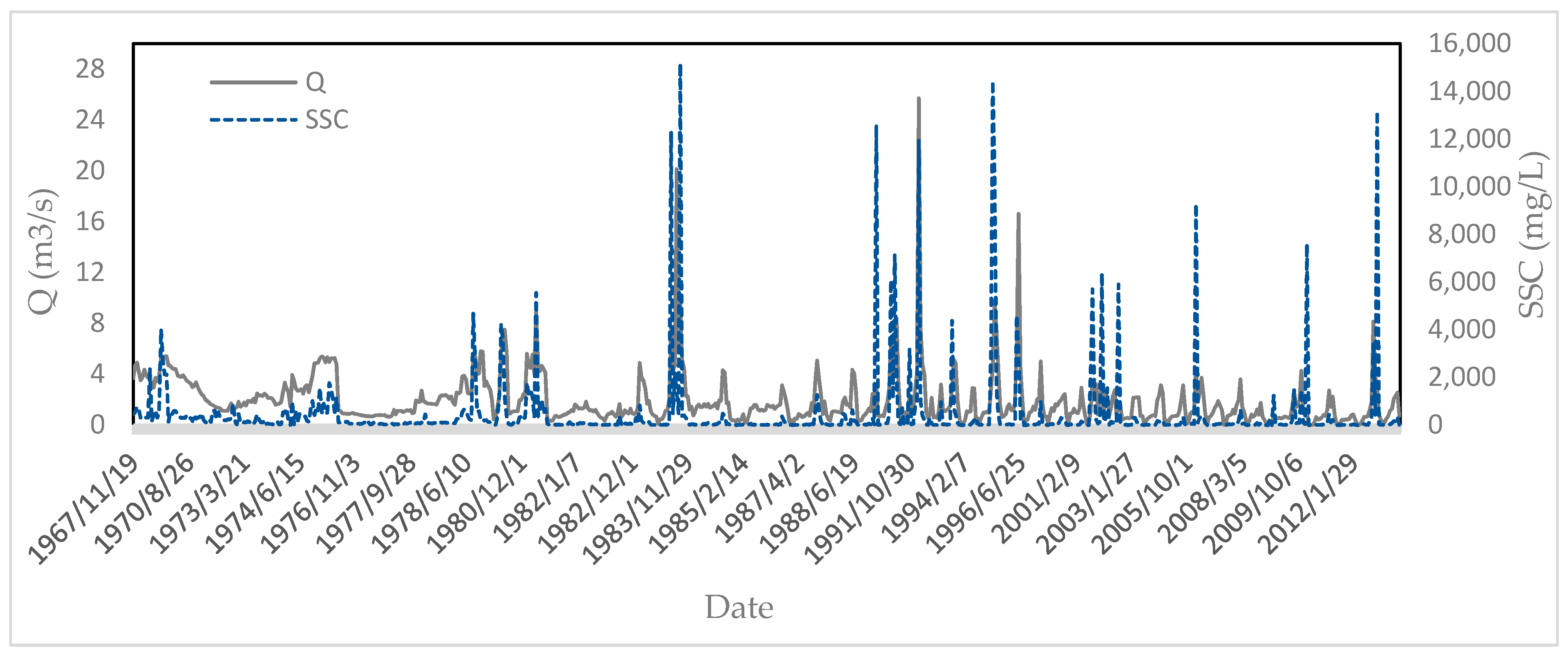
To conduct this research, Qw and SSC data for a period of 44 years (from 1969 to 2013) from Tamar hydrometric station (located at the outlet) were collected and employed in modeling. The data were not completely continuous, containing numerous missing values; a total of only 687 records were used after deleting the outliers using box plots. In Iran, due to high costs and labor for conducting direct measurements, only one or two samples are collected each month. The statistical parameters of the field data used in this study are presented in Table 1. Figure 2 shows the time series graph for Qw and SSC during the statistical period. The dataset was classified in two groups at a 70:30 ratio for model building (as the training dataset) and model evaluation (as the testing dataset) in such a way that both datasets were relatively consistent in terms of statistical parameters. We tried to include the maximum and minimum data values in the training dataset. The statistical parameters for the training and testing phases are presented in Table 2 and Table 3, respectively. Because of very small and very large values and the high skewness, it can be inferred that the SSC modeling is a complex process.
Considering the high variation of data (from very small to very large values), a normalization of data could improve the modeling process [62]. Hence, all the data were normalized within the range of 0 to 1 for intelligent algorithms as follows [63,64]:
where, and represent the minimum and maximum values among the original data and and represent the normalized and original data, respectively.
3. Methodology
3.1. Sediment Rating Curve (SRC)
The most frequently used form for SRC is a power function using log-transformation and a least squares regression technique, which is defined in general terms as [13]:
where, Qw is the flow discharge (m3/s), Qs is suspended sediment concentration (mg/L) or suspended sediment discharge (metric tons/day), and the regression coefficients (a and b) can be related to characteristics of soil erodibility and fluvial erosion, respectively [65].
3.2. Optimization Tecnhiques
3.2.1. Conventional Correction Factors
Food and Agriculture Organization (FAO)
The FAO correction factor is expressed in Equation (3) and used instead of coefficient “a” in Equation (2) [31]:
where, is the mean of Qs, is the mean of Qw, and b is the coefficient used in Equation (2).
Non-Parametric Smearing Estimator (CF2)
CF2 is a non-parametric correction factor used to improve estimated values in the SRC model by determining optimal coefficient values. CF2 is calculated using Equations (4) and (5) as follows [32]:
where, n is the sample size, ei is the error term or residual for each sample, is observed suspended sediment concentration or discharge, and is estimated suspended sediment concentration or discharge. CF2 is used in SRC model as follows:
3.2.2. Metaheuristic Algorithms
Genetic Algorithm (GA)
GA as an intelligent model is a nonlinear search and optimization technique based on the concepts of natural genetics and Darwin’s evolutionary theory, which was first offered by Holland [66] in the early 1970s. The steps for conducting GA are summarized as follows [66,67]:
- Developing a set of initial random answers; these answers, which are the primary solutions to the problem, are called chromosomes and each one is made up of sets of genes. In the present study, the coefficients a and b in the SRC model are considered as genes and form a chromosome.
- Comparing, ranking, and selecting the best chromosomes; after developing the initial population of chromosomes, to determine its suitability, the efficiency of each chromosome in estimating the suspended sediment must be determined. At this point, using Equation (2) and the values of genes in each chromosome (a and b coefficients), the amount of suspended sediment for the training data is estimated. Then, the suitability of that chromosome using the objective function (root mean squared error (RMSE)) is determined as [57]:where n is the number of training data and Oi and Si are the ith observed and estimated SSC in mg/L, respectively. After determining the suitability of the initial population of chromosomes in the natural selection stage, 50% of the most inefficient chromosomes are removed from the initial population.
- Selecting pairs (parents) for reproduction; at this stage, using selection operators, a pair of chromosomes from the set of primary chromosomes in the previous stage are determined as the parents of the next generation. To accomplish this, the widely used roulette wheel selection method was applied [61]. In fact, in this method, chromosomes with more favorable answers are more likely to be selected.
- Crossover; the production of new and better chromosomes is accomplished to further investigate the solution space (space containing possible coefficients for the SRC model). In this study, the blending method was employed to combine genes in the parent chromosomes and perform the reproduction. In each generation, the number of reproductions was determined by a parameter called the crossover rate.
- Mutation; mutation is a mechanism that leads to a completely random change in the genes of chromosomes (answers to the problem). This prevents the early convergence and getting stuck in local minima, enabling a better search within the answers space.
- Convergence; convergence implies that the GA, by repeating successive generations, is no longer able to find better answers to the problem. There are various ways to stop the genetic algorithm, e.g., the number of repetitions of generations reaching a certain level of error and lack of significant progress in error reduction.
Particle Swarm Optimization (PSO)
The PSO algorithm, proposed by Kennedy and Eberhart [68], is a social search algorithm inspired by the swarm behavior of bird flocks or fish searching for food. The steps for performing the PSO are summarized as follows:
- Generation of the initial random population with random positions and velocities, each called a particle (a and b coefficients in the SRC model are assumed to be equivalent to one particle).
- Evaluation of the cost or fitness of each particle; at this stage, the amount of suspended sediment for the training dataset is estimated using Equation (2) and the values for each particle (a and b coefficients). Then, their suitability is evaluated using the objective function (Equation (7)).
- Recording the best position for each particle (pbest) and the best position among all particles (gbest); at this step, each particle moves at a speed that can be adjusted to the search space and retains the best previous position in its memory. In addition, in the total search space, the best gained position by the group is shared with all particles. Each particle in an assumed space is shown as a position and velocity vector. The position of each particle is obtained by comparison between the current position and the best value it has achieved (pbest). Moreover, the best response that each particle has attained so far from the pbest is identified as gbest;
- Updating the position and velocity vector of all particles; in this step, the transition of the particles to new positions is evaluated. In addition, the velocity and position of each particle are corrected by Equations (8) and (9), respectively.where pbest and gbest represent the best personal position and the best position among the entire particles, respectively, t represents the number of iterations, R1 and R2 are learning parameters which determine the movement slope of the local search, and ω is the inertia coefficient.
- Convergence test; this algorithm is repeated for a predetermined number of generations or it is executed until the problem converges to an optimal solution.
Imperialist Competitive Algorithm (ICA)
The ICA proposed by Atashpaz-Gargari and Lucas [69] solves complex optimization problems by imitating the process of social, economic, and political evolution of countries. The steps for performing the ICA are summarized as follows:
- Generating the random initial countries (a and b coefficients in the SRC model are assumed equivalent to one country).
- Dividing the countries into two categories based on the objective function of the problem (Equation (7)). Countries with the lowest amounts of objective function are assumed as imperialist and the rest are colonies.
- Determining the number of colonies of each imperialist; to this aim, the power of each imperialist must be evaluated. It is obvious that the stronger the imperialist, the greater the number of its colonies.
- Applying the assimilation policy after the formation of the initial empires; in this algorithm, the assimilation policy is modeled as the movement of colonies towards imperialists.
- Revolution in countries can be considered as a sudden and accidental change in the situation of the colonized countries.
- Comparing the colonies and imperialists (intra-group competition); sometimes a colony, by moving towards an imperialist, reaches a new situation in which it has a lower cost function than the imperialist. In this case, the colony and the imperialist change positions.
- Evaluation of empires (intergroup competition); at this stage, a colony is removed from a weaker empire and transferred to another empire. If the empire has no colony, its imperialist is transferred as a colony to another empire. As a result, during colonial competition, the power of larger empires gradually increases, and weaker empires will be eliminated.
- Finally, continuing the algorithm until the termination condition is observed. The end limit of colonial competition is when we have a single empire in the world with colonies that are very close to the imperialist country in terms of situation.
In optimization algorithms, there are parameters whose changes will affect the performance of the algorithm, the convergence speed, and the quality of solutions [70]. In our study, parameters in the GA, PSO, and ICA were adjusted through trial and error as follows:
For GA: the number of initial chromosomes or size of population = 100, crossover rate = 0.75, mutation rate = 0.1, and maximum number of iterations = 500. For PSO: the number of initial particles = 100, learning parameters (R1 and R2) = 2, the inertia coefficient (ω) = 0.7, and maximum number of iterations = 500. For ICA: the number of initial countries = 100, the number of initial imperialist countries = 20, colony assimilation coefficient = 2, revolution probability = 0.1, and the maximum number of iterations = 500.
3.3. Data Separation Techniques
Considering the role of seasonal changes and river flow dynamics on sediment yield and transport at a watershed scale, data were subdivided and separated into four groups to increase the efficiency of SRC and SVR models as follows:
- Seasonal: The measured data for SSC were classified into spring, summer, autumn, and winter [71];
- Discharge classes: Data were divided based on annual average discharge such that in the first category discharge was less than average discharge; in the second category, discharge was ≥the average, but less than twice the average; in the third category, discharge was ≥twice the average [72];
- High water and low water periods: Mean monthly discharge was compared to the mean annual discharge. The months in which mean discharge was ≥ mean annual discharge were considered as the high water period and the months in which the mean discharge was less than the mean annual were considered as the low water period [73];
- Hydrograph state: The daily hydrograph of each water year was plotted and data were classified into three series based on rising and falling limbs or base flow of the hydrograph [23]. Moreover, to assess the effect of these groups on the efficiency of models in estimating suspended sediment, results were compared with a group without data separation (group 5).
3.4. Machine Learning (ML) Model
The SVR model has been successfully applied as an ML model in geoscience. Vapnik et al. [74] proposed a version of the support vector machine (SVM) that performed regression instead of classification, known as the SVR model. In fact, the same separator hyperplane in SVM becomes the fitting function of data, which has the same properties. In general, the use of the structural risk minimization (SRM) principle in the SVR modeling process equips this model with a powerful tool for generalization [75]. In this model, when a line is fitted to data, the model error can be partially ignored and the error in the calculated data must be within a range of ε that is marginal on both sides. That is, if the calculated data are within this range, the model is acceptable. However, if data are outside this range and their error is greater than ε, it must be adjusted. The SVR function can be calculated using kernel functions as follows:
where y is output, b is the bias term, α is Lagrange multiplier, and k(x,xi) is the kernel function. In our study, the SVR model was tested using the radial basis function (RBF) kernel, which has proven better in performance than other kernel functions and is currently the most widely used function [44,76], as follows [77]:
Optimal values of the kernel parameters, namely width of the Gaussian kernel function , cost of constraint violation (C), and error insensitive zone (ε), were determined by trial and error.
3.5. Model Evaluation and Comparison
Finally, to compare the results and evaluate efficiency of the models, the graphical method of scatter-plot was used and four different types of quantitative statistics, including RMSE, mean absolute error (MAE), Nash–Sutcliffe (NS) model performance coefficient, and coefficient of determination (R2) were calculated as follows [57]:
where, and are the average of observed and estimated SSC, respectively. Higher and lower R2 values represent more and less correlation between estimated and observed values. The RMSE ranges from 0 to +∞, with 0 indicating a perfect match of estimated and observed values. The range of NS values is from −∞ to 1 with being considered as acceptable model performance [45].
4. Results and Discussion
4.1. Results of the SRC Model Based on Data Separation and Non-Separation
To estimate suspended sediment using SRC, Qw and SSC were log-transformed prior to the analysis. Then, a regression relationship for each of the groups in Section 3.3 between log Qw and log SSC was established based on the training dataset. Finally, the anti-log was calculated and the ‘’a’’ and ‘’b’’ coefficients in the SRC model (i.e., Equation (2)) were determined (Table 4).
After extracting the SRC equations, the efficiency and accuracy of each equation was evaluated based on testing data in each group (Table 5). Based on these results, SRC without data separation had the lowest estimation power (NS = 0.19), while data separation significantly improved model performance. Based on these findings, SRC with NS = 0.44 had the highest estimation power in winter and the lowest estimation power in summer. This may be related to the dry conditions and short-term heavy rains in summer complicating the SSC patterns. Furthermore, results revealed that SRC was much more effective when Qw was lower than the mean Qw (NS = 0.29) and in low water period (NS = 0.33). Overall, estimated values were in closer agreement with observed values for lower flow discharge than for higher discharge.
According to the hydrograph, the SCR had the lowest performance in the falling limb (NS = 0.13). Notably, for the same Qw, SSC varies between rising and falling limbs, lower in the falling limb, which complicates the SSC process, hence weakening the modeling performance.
4.2. Results of Optimization of the SRC Using Classical Methods and Metaheuristic Algorithms
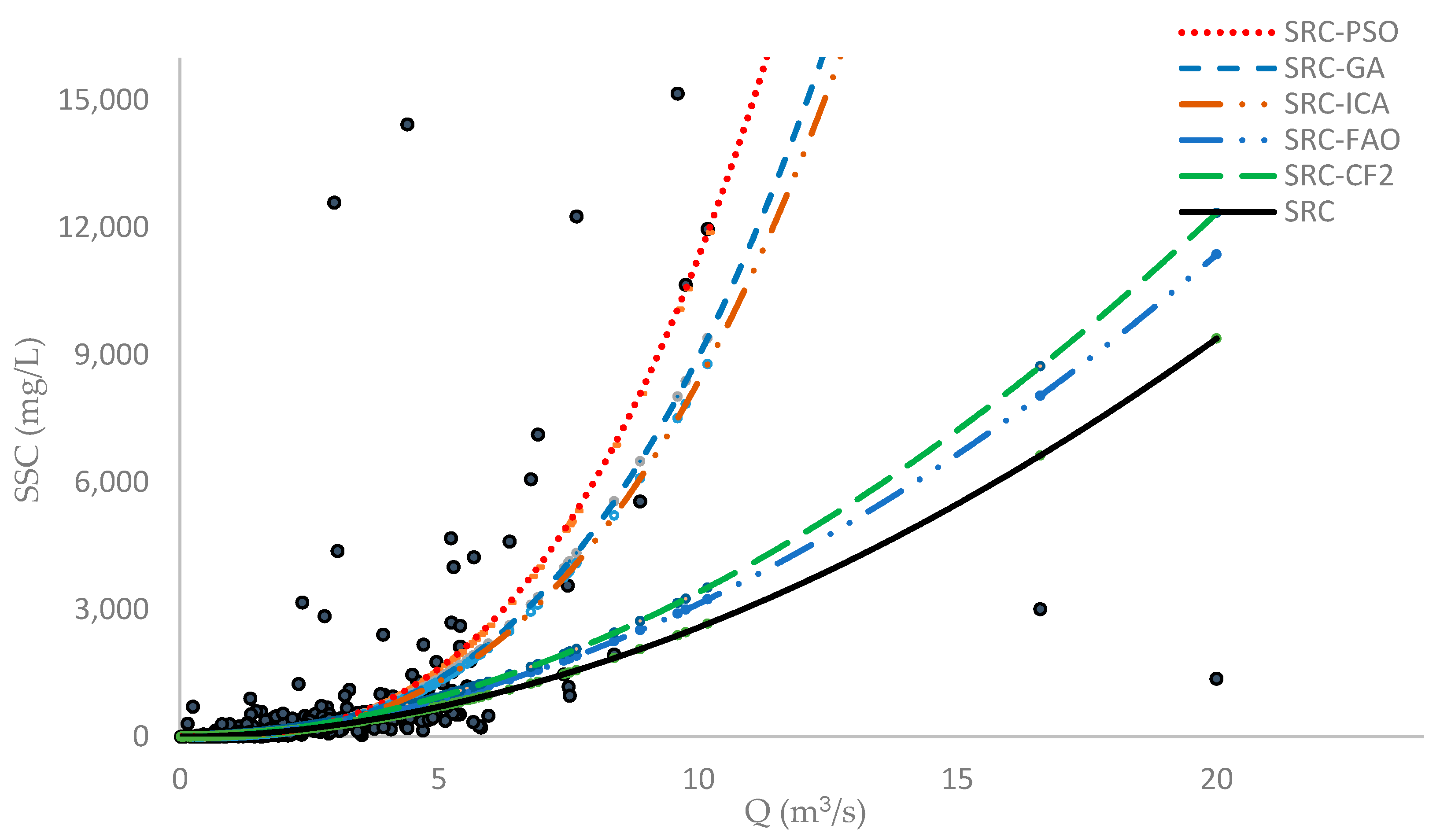
SSC was estimated using SRC models modified by two classic methods (namely, FAO and CF2) and three metaheuristic algorithms (namely, GA, PSO, and ICA) without data separation with the aim of only modifying the SRC coefficient to improve its efficiency. To this goal, after establishing a regression relationship between log Qw and log SSC during the training phase and determining ‘’a’’ and ‘’b’’ coefficients; these coefficients were modified using the previously discussed classical techniques. Optimization of the coefficients using algorithms of GA, PSO, and ICA was conducted without log-transforming data using RMSE as the objective function in the Matlab environment. After modifying the SRC equations at this stage, the efficiency and accuracy of each equation was evaluated based on the test data (Table 6). SRC-PSO had the highest estimation capability (NS = 0.44), followed by SRC-GA (NS = 0.41), SRC-ICA (NS = 0.40), SRC-CF2 (NS = 0.29), SRC-FAO (NS = 0.25), and the original SRC (NS = 0.19). Overall, the modified SRC models using the metaheuristic algorithms achieved better results than the modified SRC models using FAO and CF2 correction factors. However, although NS was low for both methods, they improved the estimation power of the original SRC. The low NS values could be due to high sensitivity to peak values of the hydrologic models, as it used squared errors [78]. The same condition was observed with RMSE, which minimized the square of residuals, while MAE was less sensitive to large values [79]. Moreover, low NS values could originate from sparse data at high discharge as well as the large amount of missing SSC-Qw data. As previously noted, field data are available only once or twice monthly in Iran; hence, finding a robust and reliable model to estimate SSC accurately is a challenging task.
Our findings agree with those of Tabatabaei et al. [57], Pour et al. [59], Tabatabaei and Salehpour Jam [58], Ebrahimi et al. [60], and Altunkaynak [61], who also state that the metaheuristic algorithms are more efficient than classic optimization methods.
The fitness of different SRC models to observed SSC data during the training phase show that SRC-PSO, SRC-GA, and SRC-ICA all more accurately estimate SSC than other optimization models (Figure 3). Overall, the SRC-PSO model had the best fit to field observations during training and testing phases. In fact, the PSO algorithm has a better chance to move toward areas containing better solutions because of features such as constructive cooperation and shared memory between particles [80].
4.3. Results of SVR Models with Data Separation and Non-Separation
In the SVR model we developed, the input and output layers contained a neuron in which Qw was considered as an input and SSC as an output. The proper architectural structure of the SVR model, like other ML models, improves the suspended sediment estimate [63]. Therefore, we used trial and error to achieve the optimal network design and improve model performance. Considering the lowest RMSE values, the optimal values for model parameters (namely,, C and ε) were assessed for all groups (Table 7).
The SVR model was developed using the entire training dataset without any data separation; then, it was evaluated using the testing dataset. Next, it was developed based on the training dataset with separated data for various groups. Finally, estimated SSC values were evaluated using the testing dataset (Table 8). The SVR model had reasonable estimation power with the entire dataset (RMSE = 1069.89 mg/L, MAE = 201.09 mg/L, NS = 0.50 and R2 = 0.52). However, in most cases, the SVR model with separated data had better performance; additionally, it had the best performance in winter (RMSE = 796.17 mg/L, MAE = 167.85 mg/L, NS = 0.68 and R2 = 0.71) and the weakest performance (lower than the entire period) during the falling limbs of hydrographs (RMSE = 1119.2 mg/L, MAE = 237.3 mg/L, NS = 0.38 and R2 = 0.43).
4.4. Determination of the Best Method of Data Separation
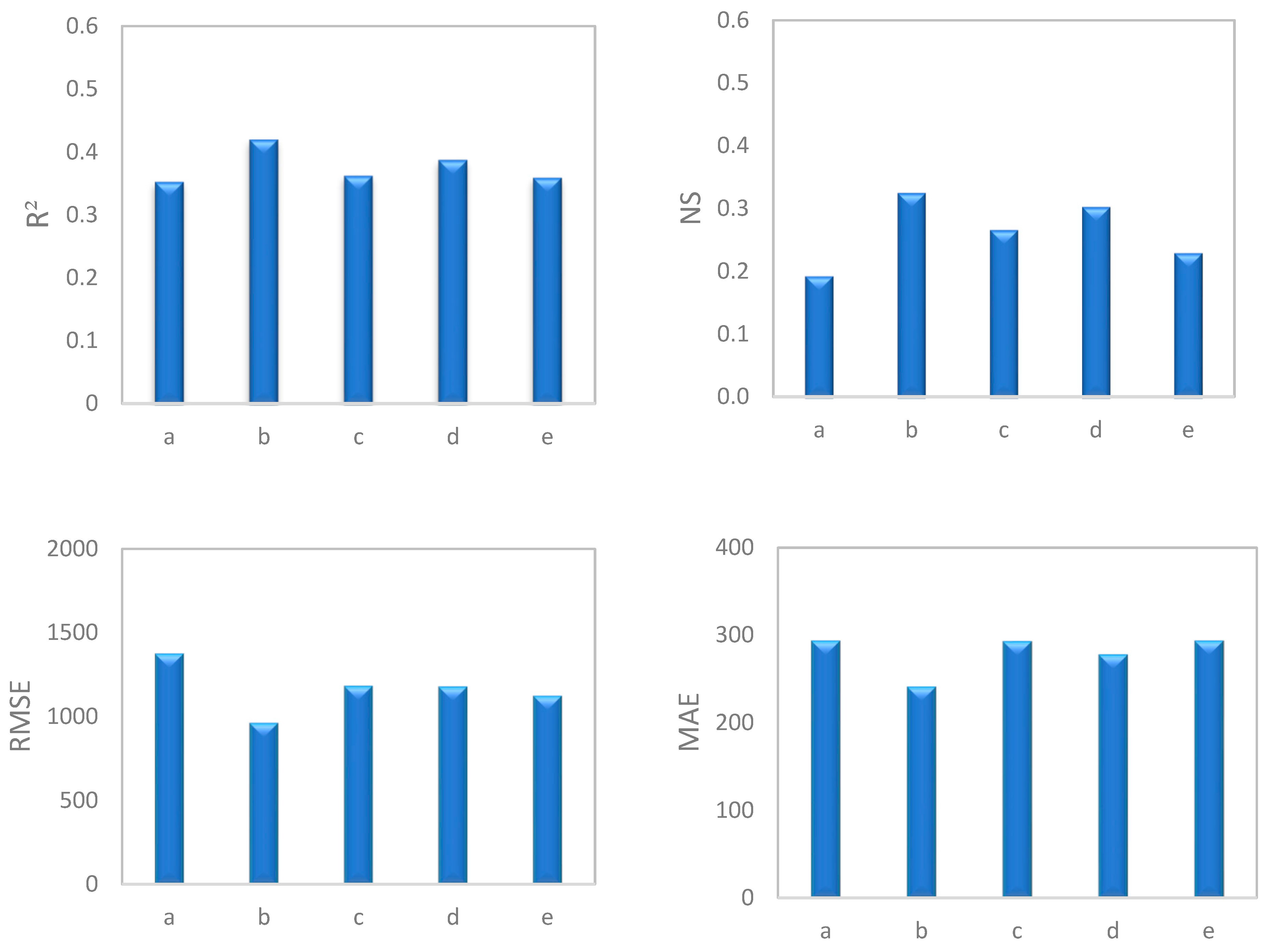
To conduct a general comparison of different groups, average values of statistical indices for seasons, discharge classes, high water and low water periods, and hydrograph state were calculated. The results revealed that in both SRC (Figure 4) and SVR (Figure 5) models, data separated by season led to the best estimation of SSC. This was followed in order by high water and low water periods, discharge classes, hydrograph state, and the original SRC. Thus, all data separation models exhibited effective performance. Research by Sichingabula [33], Horowitz [19], Collins et al. [34], Hassan [81], Zeng et al. [16], and Jung et al. [17] also confirms the greater efficiency of timely separation of data in increasing the accuracy of estimations compared with other methods of data separation.
4.5. The Most Effective Model for Estimating SSC
Based on our findings and comparing performance indices (Figure 4 and Figure 5 and Table 5, Table 6 and Table 8), the seasonal SVR model has the highest estimation power (RMSE = 819.91 mg/L, MAE = 163.58 mg/L, NS = 0.54 and R2 = 0.59) followed in order by high water/low water period SVR (NS = 0.52), discharge classes SVR (NS = 0.51), hydrograph state SVR (NS = 0.50), SVR (NS = 0.50), SRC-PSO (NS = 0.44), SRC-GA (NS = 0.41), SRC-ICA (NS = 0.40), seasonal SRC (NS = 0.32), high water/low water period SCR (NS = 0.30), SRC-CF2 (NS = 0.29), discharge classes SRC (NS = 0.26), SRC-FAO (NS = 0.25), hydrograph state SCR (NS = 0.23) and SRC (NS = 0.19).
Overall, our findings show that the SVR model presented better results in all cases with lower error values and higher NS and R2 than the SRC, including its optimized versions. In general, according to our results, the SVR model can be used to estimate SSC in similar seasons instead of applying a model for the entire dataset. Moreover, findings show that optimizing SRC through metaheuristic algorithms leads to higher performance than data separation for SRC.
In fact, the results indicate that the original SRC model could not adequately represent the complex process of suspended load in the watershed [40] because, in addition to discharge, other factors control supply and transport of suspended sediment in the watershed, such as rainfall (intensity and volume), sediment sources from previous flooding, land use/land cover changes, and anthropogenic changes in the watershed, which are not considered as model inputs. Similarly, Rodriguez et al. [29] noted that discharge only explained 19% of the variance in suspended sediment even though it is the only input to the SRC method. Another reason that the original SRC model underperforms is due to its simple structure.
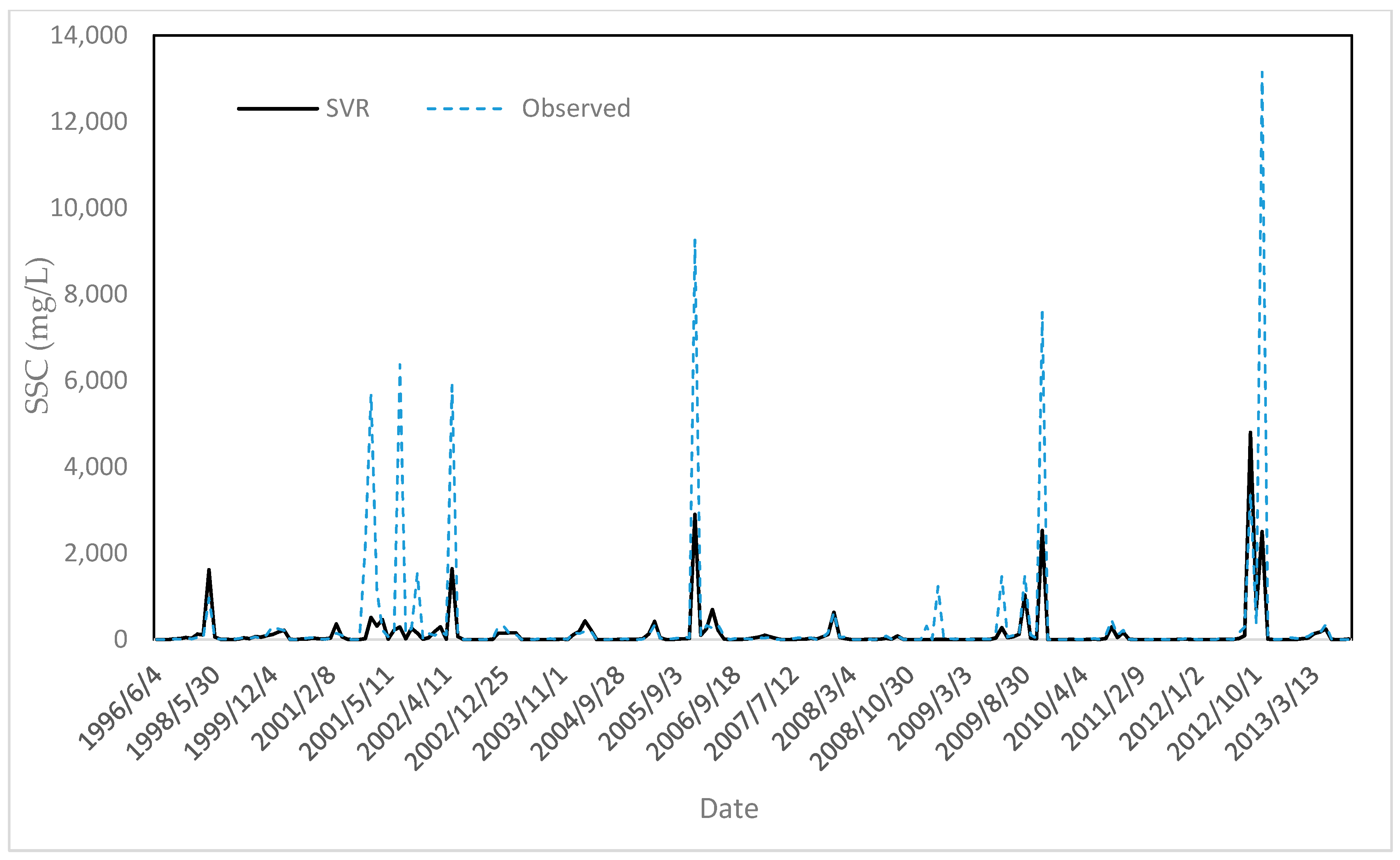
The comparison observed versus estimated SSC using the best performing models (i.e., SVR) indicates a relatively good agreement using the SVR model (Figure 6). However, as is often the case in modelling [33], peak values were not accurately estimated. This poor performance for peak value prediction is partly due to uncertainties of suspended sediment data and the low number of data samples at high discharge. Additionally, missing values can significantly affect the results. Lastly, many studies have shown that SSC cannot be estimated using only Qw [82,83].
In fact, in addition to the modeling tools [63], selection of acceptable input data can influence model results [64]. Our results showed that for accurate estimation of SSC, relevant variables other than Qw are necessary for building an effective input scenario. Several studies have shown that the utilization of antecedent values of Qw and Qs [63], meteorological parameters such as rainfall, temperature, and potential evapotranspiration [84,85], hydro-geomorphic variables such as the index of sediment connectivity [48], and biophysical data such as the normalized difference vegetation index (NDVI) [84,86], along with the hydrological parameters utilized in this study, can most likely improve estimates of suspended sediment production.
The superior performance of the SVR as a modeling tool compared to the SRC model for similar conditions (with Qw as an input and without data separation) indicates that ML models can better capture nonlinear relationships between system inputs and outputs due to their: (1) non-linear structure of the ML models, (2) robustness to missing data and (3) high flexibility [87]. Previous studies by Chiang et al. [43], Zounemat-Kermani et al. [45], Rajaee et al. [88], Muhammadi et al. [89], Kisi et al. [90], Alp and Cigizoglu [91], and Cobaner et al. [92] have also noted the superiority of ML models over traditional regression models (e.g., SRC model) for estimating suspended sediment.
5. Conclusions
Because direct measurements of fluvial suspended sediment loads are costly and time consuming, using reliable and accurate models to estimate this parameter is a challenging task for hydrologists and river engineers, especially in regions with few hydrometric stations. Our research examined and provided a reliable method that can accurately estimate SSC by: (1) optimizing SRC using metaheuristic algorithms (GA, PSO, and ICA) and classical approaches (FAO and CF2), (2) improving estimation power of SRC using separation of data based on season and flow discharge characteristics and (3) using the SVR model with only flow discharge values as inputs, similar to the SRC approach. Our findings indicate that the metaheuristic optimization algorithms are more efficient than the classic correction factors. Overall, among the metaheuristic algorithms, PSO had a higher optimization efficiency for coefficients of the SRC model. These results showed that metaheuristic algorithms could be employed instead of the classic correction coefficients and log-transformation of data in the SRC model. Moreover, to increase the accuracy of the SRC, using seasonal separation of data led to better improvements than the other methods of data separation. Overall, optimization of the SRC model using metaheuristic algorithms was more effective than data separation. The results also indicate that the SVR model had higher efficiency for estimating SSC compared to the SRC model optimized with metaheuristic algorithms.
In general, our results emphasize the benefits of using soft computing methods in enhancing the accuracy of estimating SSC. However, the SVR model predictions of SSC were not accurate when only flow discharge was used. This revealed the main weakness of the SRC method. Our improvement in suspended sediment estimation is valuable for water resources planning and management. While our results are specific to the study watershed, the possibility of extending these findings to other watersheds needs to be explored. Given that the algorithms we used were single-objective, optimization was accomplished only by minimizing the error function. Thus, we suggest surveying the multi-objective optimization algorithms (e.g., multi-objective particle swarm optimization (MOPSO)) by employing different objective functions.
Author Contributions
Formal analysis, H.A.; investigation, H.A.; Methodology, H.A., M.T.D., R.C.S., K.S.; Writing—original draft, H.A.; Writing—review and editing, M.T.D. and R.C.S. All authors have read and agreed to the published version of the manuscript.
Funding
This research received no external funding.
Institutional Review Board Statement
Not applicable.
Informed Consent Statement
Not applicable.
Data Availability Statement
This study does not report any data.
Acknowledgments
Authors would like to thank the Iran water resources management company for providing suspended sediment concentration and discharge data.
Conflicts of Interest
The authors declare no conflict of interest.
References
- Buyukyildiz, M.; Kumcu, S.Y. An estimation of the suspended sediment load using adaptive network based fuzzy inference system, support vector machine and artificial neural network models. Water Resour. Manag. 2017, 31, 1343–1359. [Google Scholar] [CrossRef]
- Sarkar, A.; Sharma, N.; Singh, R. Sediment Runoff Modelling Using ANNs in an Eastern Himalayan Basin, India. In River System Analysis and Management; Springer: Singapore; New York, NY, USA, 2017; pp. 73–82. [Google Scholar]
- Pektaş, A.O.; Doğan, E. Prediction of bed load via suspended sediment load using soft computing methods. Geofizika 2015, 32, 27–46. [Google Scholar] [CrossRef]
- Einstein, H.A. The Bed-Load Function for Sediment Transportation in Open Channel Flows; No. 1026; U.S.D.A Soil Conservation Service: Washington, DC, USA, 1950; p. 74.
- Sivapalan, M.; Takeuchi, K.; Franks, S.; Gupta, V.; Karambiri, H.; Lakshmi, V.; Liang, X.; McDonnell, J.; Mendiondo, E.; O’connell, P. IAHS Decade on Predictions in Ungauged Basins (PUB), 2003–2012: Shaping an exciting future for the hydrological sciences. Hydrol. Sci. J. 2003, 48, 857–880. [Google Scholar] [CrossRef] [Green Version]
- Cao, Z.; Li, Z.; Pender, G.; Hu, P. Non-capacity or capacity model for fluvial sediment transport. Water Manag. 2012, 165, 193–211. [Google Scholar] [CrossRef]
- Cao, Z.; Hu, P.; Pender, G. Reconciled bedload sediment transport rates in ephemeral and perennial rivers. Earth Surf. Process. Landf. 2010, 35, 1655–1665. [Google Scholar] [CrossRef]
- Hu, P.; Tan, L.; He, Z. Numerical Investigation on the Adaptation of Dam-Break Flow-Induced Bed Load Transport to the Capacity Regime over a Sloping Bed. J. Coast. Res. 2020, 36, 1237–1246. [Google Scholar] [CrossRef]
- Cao, Z.; Hu, P.; Pender, G. Multiple time scales of fluvial processes with bed load sediment and implications for mathematical modeling. J. Hydraul. Eng. 2011, 137, 267–276. [Google Scholar] [CrossRef]
- Cao, Z.; Li, Y.; Yue, Z. Multiple time scales of alluvial rivers carrying suspended sediment and their implications for mathematical modeling. Adv. Water Resour. 2007, 30, 715–729. [Google Scholar] [CrossRef]
- Yang, C.T.; Wan, S. Comparisons of selected bed-material load formulas. J. Hydraul. Eng. 1991, 117, 973–989. [Google Scholar] [CrossRef]
- Walling, D. The reliability of rating curve estimates of suspended sediment yield: Some further comments. In Sediment Budgets; IAHS Press: Porto Alegre, Brazil, 1988; pp. 337–350. [Google Scholar]
- Asselman, N. Fitting and interpretation of sediment rating curves. J. Hydrol. 2000, 234, 228–248. [Google Scholar] [CrossRef]
- Tananaev, N.I. Fitting sediment rating curves using regression analysis: A case study of Russian Arctic rivers. Proc. Int. Assoc. Hydrol. Sci. 2015, 367, 193–198. [Google Scholar] [CrossRef]
- Fan, X.; Shi, C.; Zhou, Y.; Shao, W. Sediment rating curves in the Ningxia-Inner Mongolia reaches of the upper Yellow River and their implications. Quat. Int. 2012, 282, 152–162. [Google Scholar] [CrossRef]
- Zeng, C.; Zhang, F.; Lu, X.; Wang, G.; Gong, T. Improving sediment load estimations: The case of the Yarlung Zangbo River (the upper Brahmaputra, Tibet Plateau). Catena 2018, 160, 201–211. [Google Scholar] [CrossRef]
- Jung, B.M.; Fernandes, E.H.; Möller, O.O.; García-Rodríguez, F. Estimating suspended sediment concentrations from River Discharge data for reconstructing gaps of information of long-term variability studies. Water 2020, 12, 2382. [Google Scholar] [CrossRef]
- Ulke, A.; Tayfur, G.; Ozkul, S. Predicting suspended sediment loads and missing data for Gediz River, Turkey. J. Hydrol. Eng. 2009, 14, 954–965. [Google Scholar] [CrossRef] [Green Version]
- Horowitz, A.J. An evaluation of sediment rating curves for estimating suspended sediment concentrations for subsequent flux calculations. Hydrol. Process. 2003, 17, 3387–3409. [Google Scholar] [CrossRef]
- Sadeghi, S.; Mizuyama, T.; Miyata, S.; Gomi, T.; Kosugi, K.; Fukushima, T.; Mizugaki, S.; Onda, Y. Development, evaluation and interpretation of sediment rating curves for a Japanese small mountainous reforested watershed. Geoderma 2008, 144, 198–211. [Google Scholar] [CrossRef]
- Walling, D. Suspended sediment and solid yields from a small catchment prior to urbanization. Fluv. Process. Instrum. Watersheds 1974, 6, 169–192. [Google Scholar]
- Jansson, M.B. Comparison of sediment rating curves developed on load and on concentration. Hydrol. Res. 1997, 28, 189–200. [Google Scholar] [CrossRef]
- Delmas, M.; Cerdan, O.; Cheviron, B.; Mouchel, J.-M. River basin sediment flux assessments. Hydrol. Process. 2011, 25, 1587–1596. [Google Scholar] [CrossRef]
- Ferguson, R. River loads underestimated by rating curves. Water Resour. Res. 1986, 22, 74–76. [Google Scholar] [CrossRef]
- Iadanza, C.; Napolitano, F. Sediment transport time series in the Tiber River. Phys. Chem. Earth Parts A/B/C 2006, 31, 1212–1227. [Google Scholar] [CrossRef]
- Ziegler, A.D.; Benner, S.G.; Tantasirin, C.; Wood, S.H.; Sutherland, R.A.; Sidle, R.C.; Jachowski, N.; Nullet, M.A.; Xi, L.X.; Snidvongs, A. Turbidity-based sediment monitoring in northern Thailand: Hysteresis, variability, and uncertainty. J. Hydrol. 2014, 519, 2020–2039. [Google Scholar] [CrossRef]
- Jansson, M.B. Estimating a sediment rating curve of the Reventazon river at Palomo using logged mean loads within discharge classes. J. Hydrol. 1996, 183, 227–241. [Google Scholar] [CrossRef]
- Sidle, R.C.; Campbell, A.J. Patterns of Suspended Sediment Transport in a Coastal Alaska Stream 1. JAWRA J. Am. Water Resour. Assoc. 1985, 21, 909–917. [Google Scholar] [CrossRef]
- Rodríguez-Blanco, M.; Taboada-Castro, M.; Palleiro, L.; Taboada-Castro, M. Temporal changes in suspended sediment transport in an Atlantic catchment, NW Spain. Geomorphology 2010, 123, 181–188. [Google Scholar] [CrossRef]
- Sidle, R.C. Bed load transport regime of a small forest stream. Water Resour. Res. 1988, 24, 207–218. [Google Scholar] [CrossRef]
- Jones, K.R.; Berney, O.; Carr, D.P.; Barret, E.C. Arid Zone Hydrology for Agricultural Development; FAO Irrigation and Drainage Paper No. 37; FAO: Rome, Italy, 1981. [Google Scholar]
- Duan, N. Smearing Estimate: A Nonparametric Retransformation Method. J. Am. Stat. Assoc. 1983, 78, 605–610. [Google Scholar] [CrossRef]
- Sichingabula, H.M. Factors controlling variations in suspended sediment concentration for single-valued sediment rating curves, Fraser River, British Columbia, Canada. Hydrol. Process. 1998, 12, 1869–1894. [Google Scholar] [CrossRef]
- Collins, A.; Walling, D.; Leeks, G. Use of composite fingerprints to determine the provenance of the contemporary suspended sediment load transported by rivers. Earth Surf. Process. Landf. J. Br. Geomorphol. Group 1998, 23, 31–52. [Google Scholar] [CrossRef]
- Schmidt, K.-H.; Morche, D. Sediment output and effective discharge in two small high mountain catchments in the Bavarian Alps, Germany. Geomorphology 2006, 80, 131–145. [Google Scholar] [CrossRef]
- Sadeghi, S.H.; Saeidi, P. Reliability of sediment rating curves for a deciduous forest watershed in Iran. Hydrol. Sci. J. 2010, 55, 821–831. [Google Scholar] [CrossRef]
- Harrington, S.T.; Harrington, J.R. An assessment of the suspended sediment rating curve approach for load estimation on the Rivers Bandon and Owenabue, Ireland. Geomorphology 2013, 185, 27–38. [Google Scholar] [CrossRef]
- Fang, N.; Shi, Z.; Chen, F.; Zhang, H.; Wang, Y. Discharge and suspended sediment patterns in a small mountainous watershed with widely distributed rock fragments. J. Hydrol. 2015, 528, 238–248. [Google Scholar] [CrossRef]
- Tuset, J.; Vericat, D.; Batalla, R. Rainfall, runoff and sediment transport in a Mediterranean mountainous catchment. Sci. Total Environ. 2016, 540, 114–132. [Google Scholar] [CrossRef] [PubMed]
- Hapsari, D.; Onishi, T.; Imaizumi, F.; Noda, K.; Senge, M. The use of sediment rating curve under its limitations to estimate the suspended load. Rev. Agric. Sci. 2019, 7, 88–101. [Google Scholar] [CrossRef] [Green Version]
- Zhu, Y.-M.; Lu, X.; Zhou, Y. Suspended sediment flux modeling with artificial neural network: An example of the Longchuanjiang River in the Upper Yangtze Catchment, China. Geomorphology 2007, 84, 111–125. [Google Scholar] [CrossRef]
- Melesse, A.; Ahmad, S.; McClain, M.; Wang, X.; Lim, Y. Suspended sediment load prediction of river systems: An artificial neural network approach. Agric. Water Manag. 2011, 98, 855–866. [Google Scholar] [CrossRef]
- Chiang, J.-L.; Tsai, K.-J.; Chen, Y.-R.; Lee, M.-H.; Sun, J.-W. Suspended Sediment Load Prediction Using Support Vector Machines in the Goodwin Creek Experimental Watershed. In Proceedings of the EGU General Assembly Conference Abstracts, Vienna, Austria, 27 April–2 May 2014; p. 5285. [Google Scholar]
- Kumar, D.; Pandey, A.; Sharma, N.; Flügel, W.-A. Daily suspended sediment simulation using machine learning approach. Catena 2016, 138, 77–90. [Google Scholar] [CrossRef]
- Zounemat-Kermani, M.; Kişi, Ö.; Adamowski, J.; Ramezani-Charmahineh, A. Evaluation of data driven models for river suspended sediment concentration modeling. J. Hydrol. 2016, 535, 457–472. [Google Scholar] [CrossRef]
- Khan, M.Y.A.; Tian, F.; Hasan, F.; Chakrapani, G.J. Artificial neural network simulation for prediction of suspended sediment concentration in the River Ramganga, Ganges Basin, India. Int. J. Sediment Res. 2019, 34, 95–107. [Google Scholar] [CrossRef]
- Rezaei, K.; Pradhan, B.; Vadiati, M.; Nadiri, A.A. Suspended sediment load prediction using artificial intelligence techniques: Comparison between four state-of-the-art artificial neural network techniques. Arabian J. Geosci. 2021, 14, 1–13. [Google Scholar] [CrossRef]
- Asadi, H.; Shahedi, K.; Sidle, R.C.; Kalami Heris, S.M. Prediction of Suspended Sediment Using Hydrologic and Hydrogeomorphic Data within Intelligence Models. Iran-Water Resour. Res. 2019, 15, 105–119. [Google Scholar]
- Basturk, B. An artificial bee colony (ABC) algorithm for numeric function optimization. Proceedings of IEEE Swarm Intelligence Symposium, Indianapolis, IN, USA, January 2006. [Google Scholar]
- Schwefel, H.-P. Evolution and Optimum Seeking: The Sixth-Generation; John Wiley & Sons, Inc.: Hoboken, NJ, USA, 1993. [Google Scholar]
- Ketabchi, H.; Ataie-Ashtiani, B. Evolutionary algorithms for the optimal management of coastal groundwater: A comparative study toward future challenges. J. Hydrol. 2015, 520, 193–213. [Google Scholar] [CrossRef]
- Ayvaz, M.T.; Elçi, A. A groundwater management tool for solving the pumping cost minimization problem for the Tahtali watershed (Izmir-Turkey) using hybrid HS-Solver optimization algorithm. J. Hydrol. 2013, 478, 63–76. [Google Scholar] [CrossRef]
- Srinivasan, K.; Kumar, K. Multi-objective simulation-optimization model for long-term reservoir operation using piecewise linear hedging rule. Water Resour. Manag. 2018, 32, 1901–1911. [Google Scholar] [CrossRef]
- Ebtehaj, I.; Bonakdari, H. Assessment of evolutionary algorithms in predicting non-deposition sediment transport. Urban Water J. 2016, 13, 499–510. [Google Scholar] [CrossRef]
- Ebtehaj, I.; Bonakdari, H.; Zaji, A.H.; Gharabaghi, B. Evolutionary optimization of neural network to predict sediment transport without sedimentation. Complex Intell. Syst. 2021, 7, 401–416. [Google Scholar] [CrossRef]
- Gaur, S.; Chahar, B.R.; Graillot, D. Analytic elements method and particle swarm optimization based simulation–optimization model for groundwater management. J. Hydrol. 2011, 402, 217–227. [Google Scholar] [CrossRef]
- Tabatabaei, M.; Jam, A.S.; Hosseini, S.A. Suspended sediment load prediction using non-dominated sorting genetic algorithm II. Int. Soil Water Conserv. Res. 2019, 7, 119–129. [Google Scholar] [CrossRef]
- Tabatabaei, M.; Salehpour Jam, A. Optimization of sediment rating curve coefficients using evolutionary algorithms and unsupervised artificial neural network. Casp. J. Environ. Sci. 2017, 15, 385–399. [Google Scholar]
- Pour, O.M.R.; Shui, L.T.; Dehghani, A.A. Comparision of ant colony optimization and genetic algorithm models for identifying the relation between flow discharge and suspended sediment load (Gorgan River-Iran). Sci. Res. Essays 2012, 7, 3584–3604. [Google Scholar]
- Ebrahimi, H.; Jabbari, E.; Ghasemi, M. Application of Honey-Bees Mating Optimization algorithm on Estimation of Suspended Sediment Concentration. World Appl. Sci. J. 2013, 22, 1630–1638. [Google Scholar]
- Altunkaynak, A. Sediment load prediction by genetic algorithms. Adv. Eng. Softw. 2009, 40, 928–934. [Google Scholar] [CrossRef]
- Yilmaz, B.; Aras, E.; Nacar, S.; Kankal, M. Estimating suspended sediment load with multivariate adaptive regression spline, teaching-learning based optimization, and artificial bee colony models. Sci. Total Environ. 2018, 639, 826–840. [Google Scholar] [CrossRef] [PubMed]
- Choubin, B.; Darabi, H.; Rahmati, O.; Sajedi-Hosseini, F.; Kløve, B. River suspended sediment modelling using the CART model: A comparative study of machine learning techniques. Sci. Total Environ. 2018, 615, 272–281. [Google Scholar] [CrossRef]
- Asadi, H.; Shahedi, K.; Jarihani, B.; Sidle, R.C. Rainfall-runoff modelling using hydrological connectivity index and artificial neural network approach. Water 2019, 11, 212. [Google Scholar] [CrossRef] [Green Version]
- Morgan, R.P.C. Soil Erosion and Conservation; John Wiley & Sons: Hoboken, NJ, USA, 2009. [Google Scholar]
- Holland, J.H. Outline for a logical theory of adaptive systems. J. ACM JACM 1962, 9, 297–314. [Google Scholar] [CrossRef]
- Michalewicz, Z. Genetic Algorithms+Data Structures=Evolution Programs; Springer Science & Business Media: Berlin/Heidelberg, Germany, 2013. [Google Scholar]
- Kennedy, J.; Eberhart, R. Particle swarm optimization. In Proceedings of the ICNN’95—International Conference on Neural, Networks, Perth, WA, Australia, 27 November–1 December 1995; Volume 4, pp. 1942–1948. [Google Scholar]
- Atashpaz-Gargari, E.; Lucas, C. Imperialist competitive algorithm: An algorithm for optimization inspired by imperialistic competition. Proceedings of 2007 IEEE Congress on Evolutionary Computation, Singapore, 25–28 September 2007; pp. 4661–4667. [Google Scholar]
- Bayram, A.; Uzlu, E.; Kankal, M.; Dede, T. Modeling stream dissolved oxygen concentration using teaching–learning based optimization algorithm. Environ. Earth Sci. 2015, 73, 6565–6576. [Google Scholar] [CrossRef]
- Walling, D. Assessing the accuracy of suspended sediment rating curves for a small basin. Water Resour. Res. 1977, 13, 531–538. [Google Scholar] [CrossRef]
- Preston, S.D.; Bierman, V.J., Jr.; Silliman, S.E. An evaluation of methods for the estimation of tributary mass loads. Water Resour. Res. 1989, 25, 1379–1389. [Google Scholar] [CrossRef]
- Hassanzadeh, H.; Bajestan, M.S.; Paydar, G.R. Performance evaluation of correction coefficients to optimize sediment rating curves on the basis of the Karkheh dam reservoir hydrography, west Iran. Arab. J. Geosci. 2018, 11, 1–9. [Google Scholar] [CrossRef]
- Vapnik, V. The nature of statistical learning theory. IEEE Trans. Neural Netw. 1995, 195, 5. [Google Scholar]
- Cristianini, N.; Shawe-Taylor, J. An Introduction to Support Vector Machines and Other Kernel-Based Learning Methods; Cambridge University Press: Cambridge, UK, 2000. [Google Scholar]
- Wang, H.; Xu, D. Parameter selection method for support vector regression based on adaptive fusion of the mixed kernel function. J. Control. Sci. Eng. 2017, 2017, 1–12. [Google Scholar] [CrossRef]
- Chen, S.-T.; Yu, P.-S. Pruning of support vector networks on flood forecasting. J. Hydrol. 2007, 347, 67–78. [Google Scholar] [CrossRef]
- Criss, R.E.; Winston, W.E. Do Nash values have value? Discussion and alternate proposals. Hydrol. Process. An Int. J. 2008, 22, 2723–2725. [Google Scholar] [CrossRef]
- Muleta, M.K. Model performance sensitivity to objective function during automated calibrations. J. Hydrol. Eng. 2012, 17, 756–767. [Google Scholar] [CrossRef]
- Liu, B.; Wang, L.; Jin, Y.-H.; Tang, F.; Huang, D.-X. Improved particle swarm optimization combined with chaos. Chaos Solitons Fractals 2005, 25, 1261–1271. [Google Scholar] [CrossRef]
- Hassan, S. Suspended Sediment Rating Curve for Trigis River Upstream Al-Amarah Barrage. Int. J. Adv. Res 2014, 2, 624–629. [Google Scholar]
- Nhu, V.-H.; Khosravi, K.; Cooper, J.R.; Karimi, M.; Kisi, O.; Pham, B.T.; Lyu, Z. Monthly suspended sediment load prediction using artificial intelligence: Testing of a new random subspace method. Hydrol. Sci. J. 2020, 65, 2116–2127. [Google Scholar] [CrossRef]
- Salih, S.Q.; Sharafati, A.; Khosravi, K.; Faris, H.; Kisi, O.; Tao, H.; Ali, M.; Yaseen, Z.M. River suspended sediment load prediction based on river discharge information: Application of newly developed data mining models. Hydrol. Sci. J. 2020, 65, 624–637. [Google Scholar] [CrossRef]
- Gao, G.; Ning, Z.; Li, Z.; Fu, B. Prediction of long-term inter-seasonal variations of streamflow and sediment load by state-space model in the Loess Plateau of China. J. Hydrol. 2021, 600, 126534. [Google Scholar] [CrossRef]
- Banadkooki, F.B.; Ehteram, M.; Ahmed, A.N.; Teo, F.Y.; Ebrahimi, M.; Fai, C.M.; Huang, Y.F.; El-Shafie, A. Suspended sediment load prediction using artificial neural network and ant lion optimization algorithm. Environ. Sci. Pollut. Res. 2020, 27, 38094–38116. [Google Scholar] [CrossRef] [PubMed]
- Liu, Q.; Zhang, H.; Gao, K.; Xu, B.; Wu, J.; Fang, N. Time-frequency analysis and simulation of the watershed suspended sediment concentration based on the Hilbert-Huang transform (HHT) and artificial neural network (ANN) methods: A case study in the Loess Plateau of China. Catena 2019, 179, 107–118. [Google Scholar] [CrossRef]
- Khosravi, K.; Mao, L.; Kisi, O.; Yaseen, Z.M.; Shahid, S. Quantifying hourly suspended sediment load using data mining models: Case study of a glacierized Andean catchment in Chile. J. Hydrol. 2018, 567, 165–179. [Google Scholar] [CrossRef]
- Rajaee, T.; Mirbagheri, S.A.; Zounemat-Kermani, M.; Nourani, V. Daily suspended sediment concentration simulation using ANN and neuro-fuzzy models. Sci. Total Environ. 2009, 407, 4916–4927. [Google Scholar] [CrossRef] [PubMed]
- Muhammadi, A.; Akbari, G.; Azizzian, G. Suspended sediment concentration estimation using artificial neural networks and neural-fuzzy inference system case study: Karaj Dam. Indian J. Sci. Technol. 2012, 5, 3188–3193. [Google Scholar] [CrossRef]
- Kisi, O.; Haktanir, T.; Ardiclioglu, M.; Ozturk, O.; Yalcin, E.; Uludag, S. Adaptive neuro-fuzzy computing technique for suspended sediment estimation. Adv. Eng. Softw. 2009, 40, 438–444. [Google Scholar] [CrossRef]
- Alp, M.; Cigizoglu, H.K. Suspended sediment load simulation by two artificial neural network methods using hydrometeorological data. Environ. Model. Softw. 2007, 22, 2–13. [Google Scholar] [CrossRef]
- Cobaner, M.; Unal, B.; Kisi, O. Suspended sediment concentration estimation by an adaptive neuro-fuzzy and neural network approaches using hydro-meteorological data. J. Hydrol. 2009, 367, 52–61. [Google Scholar] [CrossRef]
Figure 1.
Location of the hydrometric station and drainage network map of Boostan dam watershed.

Figure 2.
Time series graph for flow discharge and suspended sediment concentrations.

Figure 3.
Fitness of various SRC models to the training phase.

Figure 4.
Comparison of the average performance indices (RMSE, MAE, NS, and R2) for the SRC model with different methods of data separation.
Figure 4.
Comparison of the average performance indices (RMSE, MAE, NS, and R2) for the SRC model with different methods of data separation.

Figure 5.
Comparison of the average performance indices (RMSE, MAE, NS, and R2) for the SVR model with different methods of data separation.
Figure 5.
Comparison of the average performance indices (RMSE, MAE, NS, and R2) for the SVR model with different methods of data separation.
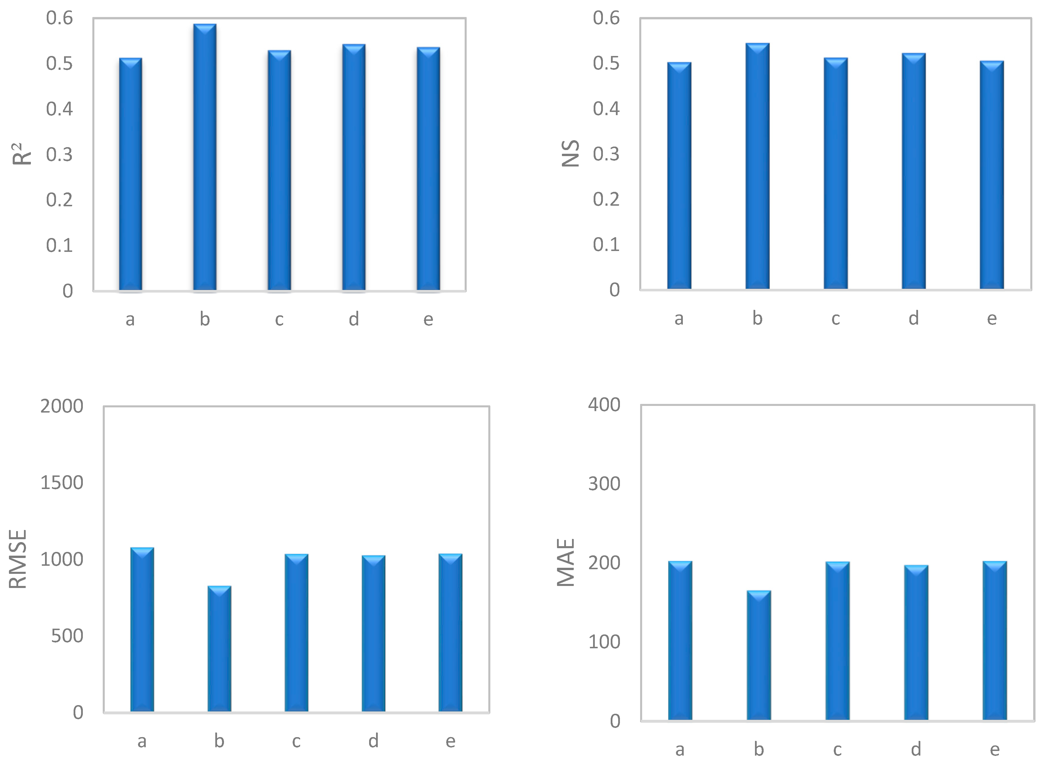
Figure 6.
Observed SSC versus estimated SSC using the best models (i.e., SVR) for the testing dataset.
Figure 6.
Observed SSC versus estimated SSC using the best models (i.e., SVR) for the testing dataset.


Table 1.
Statistical parameters of data for the studied watershed 1.
| Variable | ||||||
|---|---|---|---|---|---|---|
| (m3/s) | 0.00 | 25.71 | 1.92 | 2.04 | 4.62 | 1.06 |
| SSC (mg/L) | 0.01 | 15,152.21 | 454.41 | 1556.05 | 6.41 | 3.42 |
1 Note: is the minimum value of the data, is the maximum value, is the mean, is the standard deviation, is the skewness, is the coefficient of variation, Qw is flow discharge, and SSC is suspended sediment concentration.
Table 2.
Statistical values of Qw in the training and testing datasets 2.
| Study Period | Statistical Parameter | ||||||
|---|---|---|---|---|---|---|---|
| Dataset | |||||||
| Entire period | Training | 0 | 25.71 | 2.18 | 1.79 | 1.67 | 480 |
| Testing | 0.02 | 20.13 | 1.17 | 1.06 | 2.22 | 207 | |
| Spring | Training | 0.13 | 25.71 | 2.55 | 1.92 | 1.09 | 177 |
| Testing | 0.32 | 20.13 | 1.09 | 1.08 | 78.2 | 76 | |
| Summer | Training | 0 | 2.98 | 0.46 | 0.56 | 2.39 | 70 |
| Testing | 0.02 | 0.96 | 0.39 | 0.26 | 0.45 | 31 | |
| Autumn | Training | 0.19 | 3.18 | 0.87 | 0.42 | 2.24 | 84 |
| Testing | 0.45 | 2.36 | 1.06 | 0.42 | 0.87 | 36 | |
| Winter | Training | 0.42 | 16.6 | 1.67 | 0.9 | 2.42 | 149 |
| Testing | 0.68 | 10.48 | 2.07 | 1.43 | 2.2 | 64 | |
| Training | 0 | 2.42 | 0.63 | 0.47 | 1.15 | 236 | |
| Testing | 0.02 | 2.3 | 0.96 | 0.44 | 0.31 | 102 | |
| Training | 0.62 | 5.95 | 2.13 | 0.87 | 1.59 | 126 | |
| Testing | 0.84 | 4.44 | 2.04 | 0.93 | 0.83 | 55 | |
| Training | 1.84 | 25.71 | 4.56 | 1.42 | 2 | 117 | |
| Testing | 1.36 | 20.13 | 4.43 | 2.34 | 0.93 | 51 | |
| High water period | Training | 0.07 | 25.71 | 3.1 | 1.95 | 1.3 | 215 |
| Testing | 0.06 | 20.13 | 2.06 | 1.55 | 1.9 | 93 | |
| Low water period | Training | 0 | 5.41 | 1.31 | 1 | 2.01 | 265 |
| Testing | 0.02 | 4.31 | 0.68 | 0.58 | 2.59 | 114 | |
| Rising limb | Training | 0.65 | 25.71 | 2.85 | 1.58 | 1.46 | 142 |
| Testing | 0.72 | 16.6 | 3.26 | 2.28 | 1.43 | 62 | |
| Falling limb | Training | 0.13 | 9.6 | 2.32 | 1.86 | 1.22 | 118 |
| Testing | 0.24 | 7.41 | 1.85 | 1.49 | 1.42 | 51 | |
| Base flow | Training | 0 | 7.65 | 1.17 | 0.88 | 3.75 | 220 |
| Testing | 0.02 | 4.31 | 0.63 | 0.57 | 3.06 | 94 | |
2 Note: is the minimum value of the data, is the maximum value of the data, is the mean of the data, is the standard deviation, is the skewness, is the amount of data.
Table 3.
Statistical values of SSC for the training and testing datasets 3.
| Study Period | Statistical Parameter | ||||||
|---|---|---|---|---|---|---|---|
| Dataset | |||||||
| Entire period | Training | 0.13 | 15,152.21 | 497.17 | 1602.92 | 6.84 | 480 |
| Testing | 0.01 | 13,152.13 | 354.83 | 1439.82 | 6.16 | 207 | |
| Spring | Training | 0.39 | 15,152.21 | 944.54 | 2342.31 | 5.02 | 191 |
| Testing | 4.22 | 7585.72 | 278.85 | 1080.45 | 6.17 | 82 | |
| Summer | Training | 0.01 | 6583.52 | 162.99 | 1080.19 | 5.43 | 56 |
| Testing | 0.17 | 444.88 | 69.09 | 111.95 | 1.45 | 25 | |
| Autumn | Training | 0.14 | 5894.95 | 273.23 | 1096.45 | 4.61 | 84 |
| Testing | 0.92 | 2140.45 | 103.51 | 326.98 | 4.90 | 36 | |
| Winter | Training | 1.93 | 12,256.62 | 293.73 | 1334.35 | 7.51 | 149 |
| Testing | 5.52 | 6065.7 | 597.12 | 1286.53 | 2.80 | 64 | |
| Training | 0.01 | 7585.72 | 92.2 | 709.85 | 10.59 | 264 | |
| Testing | 0.13 | 2140.45 | 67.24 | 167.42 | 8.38 | 114 | |
| Training | 0.14 | 13,152.13 | 1257.3 | 3357.62 | 3.51 | 126 | |
| Testing | 4.22 | 12,583.52 | 379.23 | 1257.41 | 8.00 | 55 | |
| Training | 34.77 | 15,152.21 | 1159.2 | 2140.72 | 4.92 | 90 | |
| Testing | 59.82 | 11,964.84 | 1697.5 | 2797.51 | 2.54 | 38 | |
| High water period | Training | 0.14 | 15,152.21 | 611.06 | 2028.42 | 6.35 | 215 |
| Testing | 0.39 | 13,152.13 | 884.83 | 2270.51 | 4.57 | 93 | |
| Low water period | Training | 0.01 | 8231.67 | 264.22 | 1257.81 | 5.91 | 265 |
| Testing | 0.13 | 3996.55 | 147.39 | 413.62 | 6.40 | 114 | |
| Rising limb | Training | 5.5 | 14,426.4 | 1387.2 | 2910.18 | 3.07 | 142 |
| Testing | 6.73 | 4673.56 | 462.44 | 733.04 | 3.4 | 62 | |
| Falling limb | Training | 0.39 | 15,152.21 | 646.2 | 2566.84 | 5.73 | 118 |
| Testing | 0.79 | 13,152.13 | 473.59 | 1537.42 | 8.02 | 51 | |
| Base flow | Training | 0.01 | 12,583.52 | 288.15 | 1386.16 | 7.2 | 220 |
| Testing | 0.13 | 8231.67 | 135.81 | 955.45 | 9.47 | 94 | |
3 Note: is the minimum value of the data, is the maximum value, is the mean, is the standard deviation, is the skewness, is the amount of data.
Table 4.
Coefficients of the SRC equations in each of the data separation methods for the training dataset.
Table 4.
Coefficients of the SRC equations in each of the data separation methods for the training dataset.
| Group | Study Period | Equation | a | b |
|---|---|---|---|---|
| Without any separation (a) | Entire period | 35.04 | 1.86 | |
| Spring | 34.43 | 1.97 | ||
| Seasonal (b) | Summer | 32.88 | 1.36 | |
| Autumn | 29.51 | 1.81 | ||
| Winter | 17.45 | 2.66 | ||
| 31.69 | 1.48 | |||
| Discharge Classes (c) | 15.92 | 2.8 | ||
| 11.29 | 2.69 | |||
| High water-low water periods (d) | High water period | 25.46 | 2.18 | |
| Low water period | 35.21 | 1.69 | ||
| Rising limb | 22.64 | 2.31 | ||
| Hydrograph State (e) | Falling limb | 60.58 | 1.54 | |
| Base flow | 27.94 | 1.69 |
Table 5.
Evaluation of various SRC models during the testing phase.
| Model | Study Period | RMSE (mg/L) | NS | MAE (mg/L) | R2 |
|---|---|---|---|---|---|
| without any separation | Entire period | 1366.96 | 0.19 | 292.23 | 0.35 |
| Spring | 1093.17 | 0.31 | 279.18 | 0.36 | |
| Seasonal | Summer | 683.8 | 0.20 | 201.08 | 0.31 |
| Autumn | 1083.25 | 0.34 | 219.17 | 0.41 | |
| Winter | 950.22 | 0.44 | 258.69 | 0.59 | |
| 1118.38 | 0.29 | 267.99 | 0.40 | ||
| Discharge Classes | 1148.47 | 0.26 | 275.73 | 0.36 | |
| 1255.92 | 0.24 | 330.71 | 0.32 | ||
| High water/low water periods | High water period | 1189.56 | 0.27 | 287.07 | 0.36 |
| Low water period | 1151.44 | 0.33 | 265.54 | 0.41 | |
| Rising limb | 926.33 | 0.30 | 232.77 | 0.45 | |
| Hydrograph State | Falling limb | 1310.15 | 0.13 | 399.12 | 0.24 |
| Base flow | 1109.78 | 0.25 | 244.75 | 0.38 |
Table 6.
Evaluation results for various SRC models during the testing phase.
| Model Name | Equation | RMSE (mg/L) | NS | MAE (mg/L) | R2 |
|---|---|---|---|---|---|
| SRC | 1366.96 | 0.19 | 292.23 | 0.34 | |
| SRC-FAO | 1345.72 | 0.25 | 289.1 | 0.35 | |
| SRC-CF2 | 1335.75 | 0.29 | 288.2 | 0.36 | |
| SRC-PSO | 1099.91 | 0.44 | 236.95 | 0.45 | |
| SRC-GA | 1113.31 | 0.41 | 245.84 | 0.43 | |
| SRC-ICA | 1127.92 | 0.40 | 250.07 | 0.42 |
Table 7.
Optimal values for the parameters of the SVR model 4.
| Model | Study Period | SVR | ||
|---|---|---|---|---|
| C | ε | |||
| without any separation | Entire period | 2.5 | 1 | 0.1 |
| Spring | 0.3 | 5 | 0.001 | |
| Seasonal | Summer | 2 | 2.5 | 0.0001 |
| Autumn | 0.4 | 5 | 0.001 | |
| Winter | 0.1 | 1 | 0.01 | |
| 0.15 | 1 | 0.1 | ||
| Discharge Classes | 0.1 | 3.5 | 0.001 | |
| 0.17 | 5 | 0.01 | ||
| High water-low water periods | High water period | 2 | 2.5 | 0.1 |
| Low water period | 0.1 | 1 | 0.01 | |
| Rising limb | 0.21 | 1 | 0.01 | |
| Hydrograph State | Falling limb | 0.1 | 1.5 | 0.1 |
| Base flow | 0.1 | 5 | 0.0001 | |
4 Note: C is cost of constraint violation, ε is error insensitive zone, and is width of the Gaussian kernel function.
Table 8.
Evaluation of SVR models during the testing phase.
| Model | Study Period | RMSE (mg/L) | NS | MAE (mg/L) | R2 |
|---|---|---|---|---|---|
| without any separation | Entire period | 1069.89 | 0.50 | 201.09 | 0.52 |
| Spring | 1063.77 | 0.52 | 199.19 | 0.55 | |
| Seasonal | Summer | 461.86 | 0.41 | 101.77 | 0.45 |
| Autumn | 957.84 | 0.56 | 185.5 | 0.63 | |
| Winter | 796.17 | 0.68 | 167.85 | 0.71 | |
| 970.86 | 0.55 | 182.83 | 0.56 | ||
| Discharge Classes | 1023.99 | 0.52 | 200.08 | 0.54 | |
| 1088.75 | 0.46 | 217.38 | 0.48 | ||
| High water—low water periods | High water period | 1106.5 | 0.51 | 201.63 | 0.53 |
| Low water period | 929.72 | 0.53 | 189.78 | 0.55 | |
| Rising limb | 911.29 | 0.57 | 171.63 | 0.59 | |
| Hydrograph State | Falling limb | 1119.2 | 0.38 | 237.3 | 0.43 |
| Base flow | 1059.23 | 0.56 | 193.46 | 0.58 |
Publisher’s Note: MDPI stays neutral with regard to jurisdictional claims in published maps and institutional affiliations. |
© 2021 by the authors. Licensee MDPI, Basel, Switzerland. This article is an open access article distributed under the terms and conditions of the Creative Commons Attribution (CC BY) license (https://creativecommons.org/licenses/by/4.0/).
Share and Cite
MDPI and ACS Style
Asadi, H.; Dastorani, M.T.; Sidle, R.C.; Shahedi, K. Improving Flow Discharge-Suspended Sediment Relations: Intelligent Algorithms versus Data Separation. Water 2021, 13, 3650. https://doi.org/10.3390/w13243650
AMA Style
Asadi H, Dastorani MT, Sidle RC, Shahedi K. Improving Flow Discharge-Suspended Sediment Relations: Intelligent Algorithms versus Data Separation. Water. 2021; 13(24):3650. https://doi.org/10.3390/w13243650
Chicago/Turabian StyleAsadi, Haniyeh, Mohammad T. Dastorani, Roy C. Sidle, and Kaka Shahedi. 2021. "Improving Flow Discharge-Suspended Sediment Relations: Intelligent Algorithms versus Data Separation" Water 13, no. 24: 3650. https://doi.org/10.3390/w13243650
Note that from the first issue of 2016, this journal uses article numbers instead of page numbers. See further details here.