
Multivariate Analysis of Water Quality Measurements on the Danube River


1
Faculty of Civil Engineering Subotica, University of Novi Sad, Kozaracka 2a, 24000 Subotica, Serbia
2
Faculty of Technology Novi Sad, University of Novi Sad, Bulevar cara Lazara 1, 21000 Novi Sad, Serbia
3
Faculty of Agriculture, University of Novi Sad, Trg Dositeja Obradovića 8, 21000 Novi Sad, Serbia
4
Faculty of Health, Jaume I University, Avinguda de Vicent Sos Baynat, s/n, 12071 Castelló de la Plana, Spain
5
Department of Engineering Management in Biotechnology, Faculty of Economics and Engineering Management in Novi Sad, University Business Academy in Novi Sad, Cvećarska 2, 21000 Novi Sad, Serbia
*
Author to whom correspondence should be addressed.
Water 2021, 13(24), 3634; https://doi.org/10.3390/w13243634
Submission received: 16 November 2021
/
Revised: 15 December 2021
/
Accepted: 16 December 2021
/
Published: 17 December 2021
(This article belongs to the Special Issue Chemical and Biological Methods in Aquatic Ecosystem Status Assessment)
Abstract
:This study investigates the potential of using principal component analysis and other multivariate analysis techniques to evaluate water quality data gathered from natural watercourses. With this goal in mind, a comprehensive water quality data set was used for the analysis, gathered on a reach of the Danube River in 2011. The considered measurements included physical, chemical, and biological parameters. The data were collected within seven data ranges (cross-sections) of the Danube River. Each cross-section had five verticals, each of which had five sampling points distributed over the water column. The gathered water quality data was then subjected to several multivariate analysis techniques. However, the most attention was attributed to the principal component analysis since it can provide an insight into possible grouping tendencies within verticals, cross-sections, or the entire considered reach. It has been concluded that there is no stratification in any of the analyzed water columns. However, there was an unambiguous clustering of sampling points with respect to their cross-sections. Even though one can attribute these phenomena to the unsteady flow in rivers, additional considerations suggest that the position of a cross-section can have a significant impact on the measured water quality parameters. Furthermore, the presented results indicate that these measurements, combined with several multivariate analysis methods, especially the principal component analysis, may be a promising approach for investigating the water quality tendencies of alluvial rivers.
1. Introduction
Considering the importance of water in the proper functioning of the Earth’s ecosystem, it is no wonder that water quality issues have received more and more attention in the last decades. As a result of the poor water quality, modern society faces water scarcity problems. It is not just the amount of water that needs to be accessible, but the water quality must be adequate for the intended use. Consequently, the acquisition of water-related data is becoming more critical as it can provide numerous information required to ensure potential improvement of the issue at hand. For example, knowing the sources and types of pollution entering a particular water body is the first step towards reducing or eliminating it or finding ways to mitigate the problem. Hence, it is essential to establish monitoring systems adapted to the needs of the water body at hand. According to [1], three vital tools for efficient water quality management are observation, theoretical analysis, and numerical modeling. Hence, even though data gathering is imperative and often the most challenging segment of the management process, the subsequent data analysis is critical. It contains the methodology used for proper evaluation and apprehension of the considered ecosystem and the difficulty it is facing. Proper data analysis allows researchers to determine the degree to which the water body is impaired, causes and sources of impairment, as well as possible solutions. Since the water body and the catchment surrounding it influence each other, it is often inevitable to complement the water quality analysis with the catchment’s investigation [2]. An example of water quality data analysis can be found in [3], where Yilma et al. opted for statistical methods to evaluate the water quality of the Little Akaki River.
Lake water quality monitoring is equally important. Some issues regarding this subject can be found in [4], where the Authors presented the current state, identifiable issues, and potential improvements of the Palic-Ludas Lake system in Serbia. The work published in [5] presents a case where the Authors used statistical analysis to evaluate the water quality of Lake Prashar in India. Numerous studies opt for this method because of the advantage of implementing statistical analysis to assess water quality data [6,7]. In [7], the researchers used multivariate analysis to evaluate water quality data in Lake Palic.
As suggested by [1], another essential part of water management includes establishing a numerical model that can prove advantages to the data analysis process. These models allow the user to investigate various scenarios and the expected consequences without them occurring. Some examples of numerical models are presented in [8,9]. These papers describe a two-dimensional water flow, sediment transport, and heavy metal transport models. Numerical models can provide significant advantages to any data analysis. However, they are all faced with the same disadvantage. Namely, any model is only as good as the data available to feed the model’s needs, and most often, the limitations a study faces arise from inadequate measurements. Consequently, most research, including numerical models, faces constraints due to insufficient measurements (lack of spatial or temporal data distribution, accuracy, etc.). An example of a comprehensive measuring campaign conducted on the Danube River is presented in [10]. Although it deals with hydraulic and sediment transport parameters, this paper clearly describes the extensive work required to acquire high-quality data.
After the data gathering (measurements and sampled data evaluation) is completed, an adequate tool for evaluating the available data should be selected. Since most of these measurements include large amounts of data [10], researchers often opt for multivariate techniques capable of extracting underlying information in a very efficient manner. Multivariate data analysis involves processing a substantial number of correlated variables, with different algorithms and techniques used to analyze and interpret such data. Principal component analysis (PCA) is one of the most widely used multivariate techniques in sciences, and it is being applied to wide types of datasets (e.g., sensory, instrumental methods, chemical data) [11]. It provides an overview of the complexity and interrelationships in multivariate data sets by revealing relations between variables and samples, detecting outliers, finding and quantifying patterns and trends, extracting and compressing complex datasets [12]. The theory and algorithm behind PCA can be found in [13].
Numerous researchers have chosen PCA over other alternatives because of the various benefits that this approach introduces to the data analysis. Some examples include authors Bengräine and Marhaba, who used it to study spatial and temporal changes of water quality of the Passaic River in New Jersey [14]. Using PCA, they were able to determine a point or non-point source of pollution. Ouyang [15] used PCA and factor analysis to evaluate river water quality monitoring stations (whose significance comes from the assessment of annual variations of river water quality) and to differentiate significant from irrelevant water quality parameters. Another group of authors [16] used PCA to investigate the evolution of groundwater composition in the Pisuerga river’s alluvial aquifer between two subsequent surveys. This methodology helped the authors identify a strong correlation between some considered water quality parameters and a lack of correlation between others.
Another group of authors developed a methodology for water quality prediction [17] that includes PCA as one of the steps in the established methodology. The proposed procedure was tested on the Luan River in Tangshan City. The proposed methodology uses the Lagrange interpolation method, sliding window average, and PCA for data cleaning and pretreatment. This is followed by applying one-dimensional residual convulsion neural networks and bi-directional gated recurrent units to extract local features of the water quality parameters. The considered parameters included total nitrogen, total phosphorus, and potassium permanganate index.
Considering the vast potential of PCA and other multivariate analysis techniques, this paper presents the employment of this methodology for the analysis of water quality data gathered from the Danube River. During the research presented in this paper, the main goal was to identify potential temporal and/or spatial tendencies of water quality parameters in the analyzed river reach. This was conducted by implementing box plots, normality tests for the measured parameters, correlation coefficients, and the principal component analysis. The latter was performed for each of the measured river cross-sections separately (to detect clustering by depth or by lateral position) and for the entire river reach (to detect clustering by cross-sections). The secondary goal was to develop fitted equations (models) for some of the measured water quality parameters, namely chlorophyll-a, dissolved oxygen, and pH [18,19]. To achieve this, an approach called Multivariate Polynomial Regression was used. The developed models were tested for statistical significance, the model’s residuals were tested for normality, while measurement points with high leverage were omitted in accordance with the performed multivariate analysis. To predict chlorophyll-a, virtually all the measured water quality parameters were considered. However, for the dissolved oxygen and pH models, only some of the measured parameters were considered to be predictors.
2. Materials and Methods
The water quality measurements used within this paper were conducted in 2011 on a reach of the Danube River, located between Mohacs in Hungary and Bezdan in Serbia [6,7,8]. The complete measurements included the elevations of cross-sections at approximately 100 m apart (intended for building a digital terrain model), complemented with detailed hydraulic and sediment transport measurements at seven cross-sections within the analyzed reach. A paper published by Horvat et al. [10] gives a thorough description of the hydraulic and sediment measurements implemented in addition to the water quality measurements considered in this work.
The monitored reach of the Danube River is located between rkm 1438, downstream of Mohacs in Hungary, and rkm 1432, upstream of Bezdan in Serbia. The measuring campaign included detailed data gathering from seven data ranges (cross-sections) within this reach (data range 1 was located at the upstream end, while data range 7 was located on the downstream end). Each data range contained five verticals, and every vertical had five sampling points distributed over the water column. Figure 1 shows the disposition of the data ranges and the verticals within them. Each of these points was a sampling location (vertical) where water quality data was sampled from five sampling points distributed relatively evenly throughout the water column. It should be noted that the aforementioned verticals do not stand in a perfectly straight line. This is due to the difficulties in anchoring the boats from which the sampling was conducted. Figure 1 also depicts the riverbed’s elevation. Hence, it can be stated that water quality samples were taken from both deep and shallow locations on the considered reach. This was done intentionally to get a homogeneous data set with regard to water depth.
It should be pointed out that the conducted measurements were not simultaneous but temporally distorted within five days. The location and time of measuring the seven cross-sections (data ranges) are given in Table 1.
The presented paper considers 12 water quality parameters. Water temperature T (°C) as a parameter that influences all biological processes needs to be included in any investigation concerning water quality. The pH value pH (-) was considered a measure of how acidic or alkaline the considered water body is. To monitor the dissolved solids in the water, the measurements also included electric conductivity Cond. (μS/cm). Dissolved oxygen DO (mg/L) content is important as it represents the amount of oxygen available for living organisms. Including this parameter in any water quality assessment is essential as waters with available dissolved oxygen are usually considered to be in an overall good state, as opposed to oxygen-depleted waters that usually manifest poor water quality characteristics. Aiming to complement the research with information concerning the macronutrient content, the conducted measurements also included orthophosphates marked here as PO4 (mg P/L), nitrite nitrogen marked here as NO2 (mg N/L), nitrate nitrogen marked here as NO3 (mg N/L), and ammonia nitrogen marked here as NH4 (mg N/L). To account for the presence of organic matter, chemical oxygen demand COD (mg/L) and five-day biochemical oxygen demand BOD (mg/L) was also measured. At the same time, the phytoplankton concentration is estimated via chlorophyll-a, Chl-a (μg/L). Determining the water’s transparency, i.e., turbidity, was conducted using a Secchi disk. These measurements were marked as Secchi (cm). The methods used for determining the water quality parameters are reported in Table 2. Naturally, the list given here is not final, nor should it be considered mandatory. The decision on which water quality parameters are to be monitored should be based on the characteristics of the water body in question, along with any other relevant information regarding earlier recorded pollution.
One of the key tools of the implemented analysis was determining the Pearson’s correlation coefficient to quantify the correlation between any two parameters. The Pearson’s coefficient is computed using Equation (1).
where and mark the measured values for which the correlation coefficient is to be attained, and are the corresponding average values, and denotes the number of data pairs. If the correlation coefficient’s value is less than 0.4, it indicates a low correlation; if it is between 0.4 and 0.7, it refers to a moderate correlation, between 0.7 and 0.9 a strong correlation, while for values higher than 0.9 it indicates a very strong correlation.
As a sophisticated tool of the cluster analysis inventory, the principal component analysis is used in situations where a large set of data needs to be manipulated and rearranged so that grouping (clustering) patterns can be easily identified. Using PCA, one can reduce the dimensionality of the multidimensional data set while keeping most of the variation contained in the original data set. This is achieved by finding the so-called principal components of the data set. These principal components are defined so that the first principal component will contain most of the original data’s variation. The second principal component is uncorrelated to the first one, and it contains most of the remaining data variation, and so on. The principal components are computed as a linear combination of the independent variables, in this case, the water quality parameters.
The procedure for the computation of the principal components is as follows:
- Normalization of the measured data set using Equation (2);
- Calculation of the covariance of the normalized dataset using Equation (3);
- Computing the eigenvalues of the matrix using Equation (4).
The eigenvalues attained in this manner are then rearranged in descending order, thus representing the amount of the original data’s variation in each principal component. Thus, the original multidimensional data set can be reduced to a two-dimensional data set by selecting the first two principal components. Although the dimensionality of the new data set can be higher, choosing a two (or three) dimensional data set is practical because it allows the user to easier understand the graphical representation of the data. Now, when the data points are plotted in a coordinate system defined by the first two principal components, two data points will be closer if the measurements taken there are more similar or further apart if the measurements are dissimilar. Hence, any clustering patterns become easy to detect.
The Shapiro–Wilk test was used in the presented research to test if the sample comes from a normally-distributed population (this test was used both for testing the measured parameters and the residuals of any fitted equation). The test statistic for this method is
where is the ith smallest number in the tested sample, is a measured value (i.e., a data from the sample), is the sample mean, and are the Shapiro–Wilk coefficients (computed from covariances, variances, and means of an -sized sample from a normally distributed population) [22]. Using the statistic, a -value is computed (usually using a table). As a rule, when using this test, the null hypothesis is that the sample comes from a normally distributed population. Hence, if the -value is less than the chosen confidence level, then the null hypothesis is rejected, i.e., the sample comes from a population that is not normally distributed.
The F-test is often used to compare fitted equations (models) to determine which model best fits the population from which the sample was extracted. When using this test, the null hypothesis was set to be that the tested model is no better than the null model (i.e., the population’s mean value). The significance level for all F-test conducted in this research was 5%. Since this test is commonly used in testing fitted models, it will not be detailed here, while the reader is directed to [23].
Finally, multivariate polynomial regression was used to develop fitted equations (models). This method was selected so that predictor variables could be taken into account in their polynomial form, as well as interactions between the predicting variables. For example, if there are four predicting variables, , , and , the method can consider the full interaction between these variables. This means that the fitted model can contain the following terms , , , and , i.e., all possible multiplications between the variables. The mathematical background beneath this method certainly does not fit this paper’s scope. Hence, the reader is directed to [24,25].
In the presented research, the steps for determining possible spatial/temporal tendencies were:
- Construction of box plots for each water quality parameter, separating the data by cross-sections where they were taken. This can indicate a presence of spatial tendencies on a large scale (within the entire analyzed reach).
- Testing for normality using the Shapiro–Wilk test for every measured water quality parameter regardless of where it was taken. This can indicate a presence of spatial tendencies on a large scale if the analyzed parameter does not follow the normal distribution.
- Computation of correlation coefficients between all the measured parameters to determine any tendencies within a water column, i.e., identification of possible stratification.
- PCA analysis of water quality data for each cross-section. This analysis can identify spatial tendencies within a given cross-section, i.e., lateral spatial tendencies.
- PCA analysis of water quality data for the entire reach. This analysis can identify spatial tendencies within the reach, i.e., longitudinal spatial tendencies.
In the presented research, the steps conducted for developing fitted equations (models) were:
- The appropriate potential predictor parameters are selected to develop the fitted equation. Finally, the stepwise regression method is used to select the predictor parameters to be used in the final model. During this process, each data point’s leverage and impact are monitored in order to remove data points with extremely high leverage.
- The fitted model’s correlation coefficient is computed to determine its correlation to the measured values.
- The fitted model’s statistical significance is determined using the F-test.
- The fitted model’s residuals are analyzed using the Shapiro–Wilk test (test of normality).
In this paper, the Analyse-it software package was used for all statistical and other computations.
3. Results and Discussion
The first part of the analysis included a visual inspection of the obtained data. All water quality measurements were organized in seven groups, depending on the data range (cross-section) they belong to, and represented in the form of box plots (Figure 2).
Figure 2 allows a better visual understanding of the variations of the water quality parameters between the cross-sections, i.e., spatial variations. It also provides information regarding potential similarities between the tendencies of various water quality parameters. It should be noted that the measured water depths were also subject to this inspection (Figure 2i). Naturally, the water depth cannot be considered a water quality parameter. However, Figure 2i gives information regarding the depth ranges of the sampling points in each cross-section. One can observe that the Chl-a values are quite high, but this can be attributed to the fact that the measurements were conducted in the spring (end of May), when this occurrence is frequently reported on the lower parts of the Danube River. It should also be pointed out that there is a notable increase in COD and BOD at S3, followed by an increase in NH4 at S5 and NO2 at S6. Although these results indicate a presence of a pollution source, during the measurements campaign, none could be detected. In addition, the reach is situated in a nature protection area.
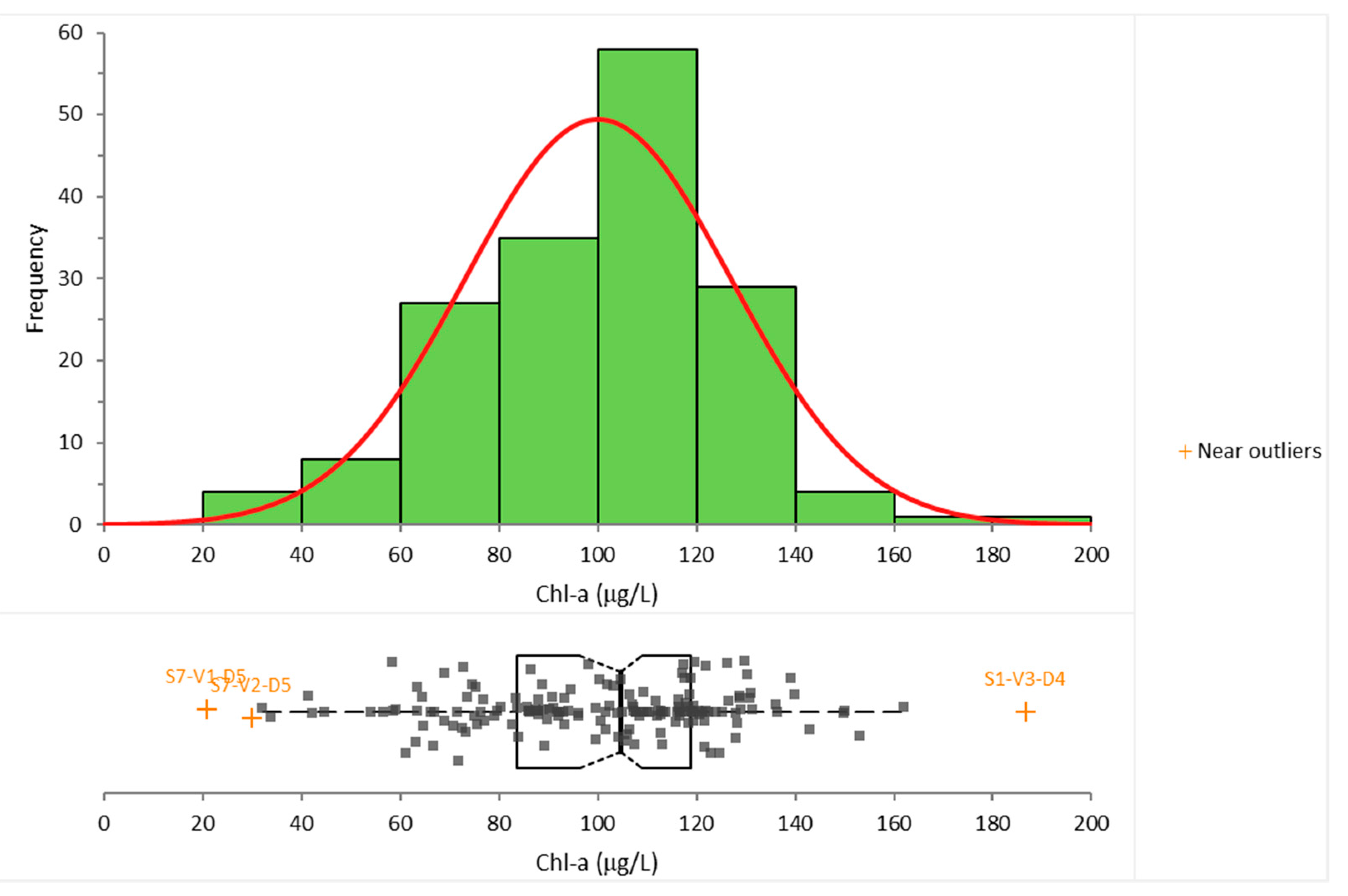
As the next step of the preformed analysis, the gathered data was organized so that all of the measurements for one water quality parameter belong to one single group, regardless of the cross-section where they were collected. These groups were then tested to whether they followed the normal distribution. If the data set follows the normal distribution, it should point to the fact that there should be no clear spatial or temporal tendencies within it. The Shapiro–Wilk test was used to test the “normality” of these data sets, alongside a plotted histogram for frequency distribution and a fitted normal distribution as a curve. Box plots were also constructed with marked outliers. An example of this is given in Figure 3 for Chlorophyll-a. All the conducted tests confirmed that neither monitored water quality parameters followed the normal distribution. This strongly suggests that there are temporal and/or spatial variations contained in the measured data sets. Hence, further analysis is justified.
The first spatial tendency that was searched for was the correlation between a particular water quality parameter and depth. The values of the computed Pearson’s correlation coefficients can be seen in Table 3. It is evident that there was no significant (positive or negative) correlation between water depth and the monitored water quality parameters. This can be attributed to the intense turbulence present in alluvial watercourses. However, it should be noted that the most considerable correlation was computed for dissolved oxygen and nitrate nitrogen, −0.17 and −0.14, respectively. These values are not sufficient even to characterize this as a moderate association between the variables, as mentioned in Section 2. Therefore, it can be concluded that the flow’s turbulence is so intense that no stratification can occur within the water column that would facilitate different conditions on different water depths.
It is also noteworthy to report that these measurements were conducted for a discharge of roughly 1600 m3/s, which is considered to be relatively low for this part of the Danube River. Although the executed measurements campaign was extensive, it certainly does not cover all possible hydraulic conditions. Hence, although it is not likely, stratification in the water column may occur in some parts of the analyzed river reach under different (much lower) discharges and (higher) temperatures.
Table 3 also gives the computed values of the correlation coefficient between all the measured water quality parameters (depth, marked d, was also added to this list). Further evaluation of the computed correlation coefficients showed that the strongest correlations were found between T and Cond (−0.815), pH and DO (0.838), Cond. and PO4 (−0.62), as well as between T and PO4 (0.583). The rest of the correlations had significantly lower values. However, the high correlation between pH and DO can be explained by the high Chl-a values (Figure 2d). Namely, increased photosynthesis generates the rise in DO values and depletes carbonate, which at constant alkalinity can produce a significant increase in pH (Figure 2a,j).
As stated in the Introduction, many researchers used PCA for analyzing water quality data. Petersen et al. [26] described an example of such an endeavor. They implemented multivariable analysis on the water quality data of River Elbe and identified two patterns. The first pattern was discharge dependent, while the other was related to biological activities. As a result, the authors suggested comparing this type of analysis with results attained by numerical models, as it could provide a better understanding of the nutrient system. In their work, Debska et al. [27] analyzed the changes in water quality parameters depending on the land use of different areas in the considered catchment. To do so, they implemented monthly measurements along the River Utrata for one year. The monitored water quality parameters included total phosphorus, ammonia nitrogen, nitrate nitrogen, dissolved oxygen, and chemical oxygen demand. After utilizing the PCA on the gathered data, they found that agricultural land use and proximity of urban areas negatively influence the river’s water quality.
Further examples of implementing multivariate analysis for water quality data manipulation can be found in [28,29,30]. The work presented in [28] describes the steps to discover changes and patterns of water quality data in the Thi Vai Estuary utilizing multivariate data analysis. Using a 15 year-long data set, the authors employed trend analysis, cluster analysis, and PCA to establish that the considered area is influenced by point and diffused pollution. The work described in [29] used PCA to evaluate the drinking water supply systems. Here the authors investigated the vulnerability of the drinking water supply system depending on various factors. Other areas of research implementing multivariate analysis include the evaluation of microplastic pollution in rivers, such as the study presented by Li et al. [30].
PCA was implemented for 12 water quality parameters for each cross-section separately. The results are presented in Figure 4. However, before these are analyzed, one should acknowledge the amount of the original data’s variation in these results. This information is given in Table 4, where it can be seen that after implementing the PCA, about 43–56% of the original variation was preserved.
To include additional information into the presented analysis, the sampling points are labeled with letters D and appropriate numbers, marking the sampling depth. By convention, D1 is the sampling point with the largest depth. The horizontal and vertical axes in Figure 4 represent the first two principal components. Considering that the principal components are a linear combination of the independent variables, they do not hold any physical meaning. The rest of the (non-horizontal and/or vertical) lines mark the axes of water quality parameters. It should be noted that only parameters with more than 50% of their original variance preserved are presented. It should be stated that this percentage only reports the fraction of the captured variance of a particular parameter, and it does not refer to that parameter’s contribution to the two main principal components. As mentioned before, the proximity of two points in Figure 4 suggests the similarity of measurements. Hence, if two sampling points are close to each other, the measured water quality parameters are similar in these two points. This aids the identification of potential grouping in the considered data set.
In Figure 4b, it can be seen that sampling points from each vertical formed their own group. This means that there was a significant similarity between points on the same vertical. Hence, it can be stated that in cross-section 2, there was a detectable distribution of water quality parameters across the cross-section’s width. Results presented in Figure 4e–g indicated that points from vertical 1 formed their own cluster. Although the results suggest some kind of distribution across the flow width, there was no identifiable clustering across the depth of any vertical. The last conclusion is in accordance with the results in Table 2. Hence, it can be stated with considerable certainty that there is no dependency between the water depth and the monitored water quality parameters.
The previously stated observations indicate that when selecting a representative sampling point (in terms of water quality parameters) for a considered cross-section, the sampling depth had virtually no importance. However, the sampling point’s location with respect to the width of the cross-section carried with it a specific risk with regards to attaining representative measurements. This can be best demonstrated using the results from Figure 4b, where it can be seen that samples taken from verticals 1 and 5 gave significantly different results. On the other hand, for cross-section 6 (Figure 4f), the differences in water quality between verticals 1 and 5 were moderate.
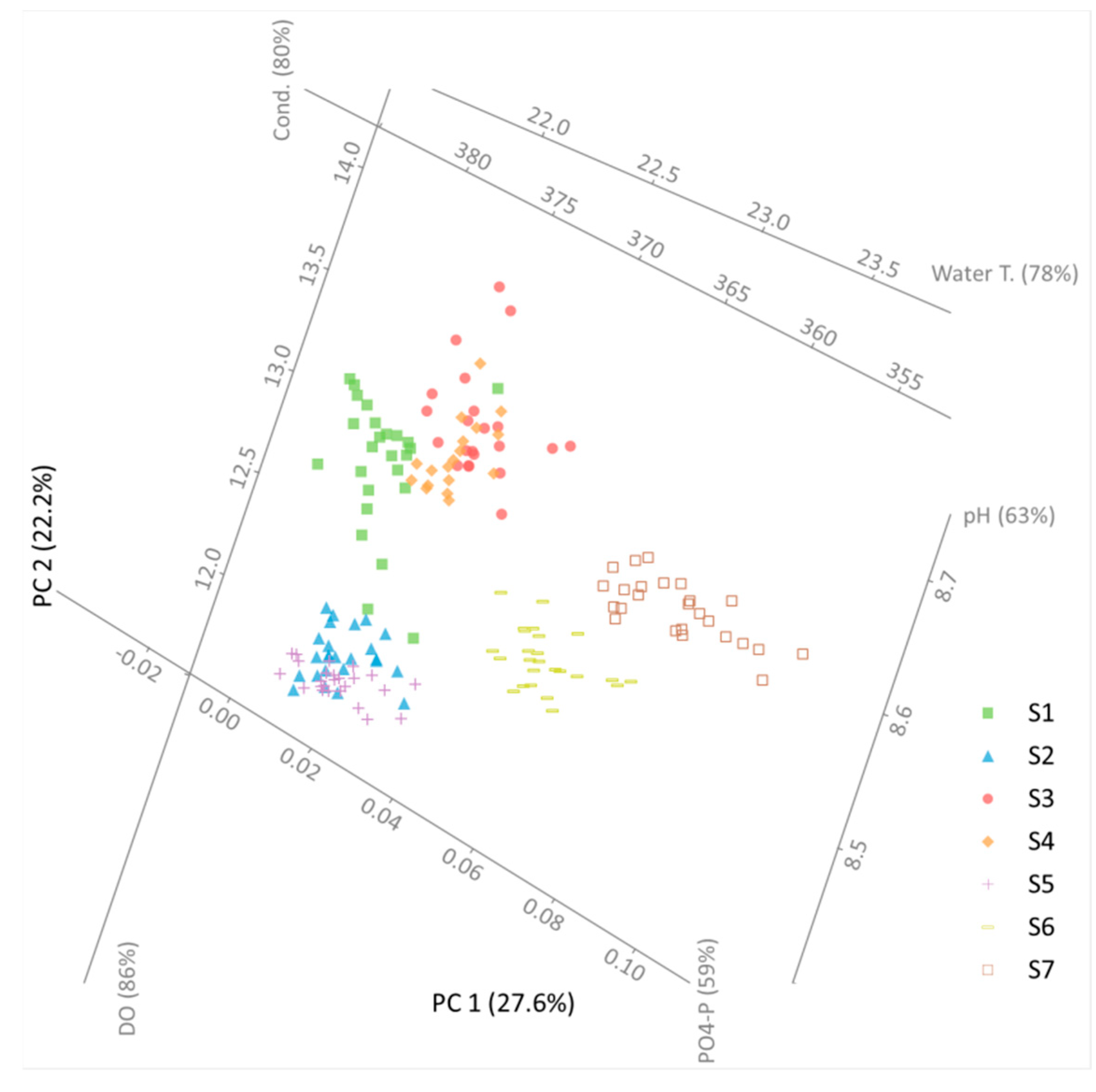
Principal component analysis was conducted on the entire data set as well, i.e., all the measured values regardless of their location were put in one data set. The aim was to investigate whether there is a similarity between sampling points within one cross-section or if no spatial grouping can be identified. The results are given in Figure 5. It should be noted that the computation indicated that 49.8% of the original data’s variation is contained in Figure 5. First of all, it can be safely stated that sampling points in every single cross-section formed their own cluster. However, it is also vital to notice that points from some cross-sections (cross-sections 1, 6, and 7) formed independent, clearly defined groups. In contrast, points from other cross-sections (at least partially) overlapped (cross-section 2 with 5 and cross-section 3 with 4). These observations should not be taken lightly because their interpretation is more complicated than it seems at first glance. As stated earlier, the samples from the analyzed cross-section were taken at different times, i.e., samples from some cross-sections were taken on the same day, while other cross-sections were processed on different days (Table 1). Hence, the measurements contained within them not only a spatial but also a temporal offset. One could argue that the existing temporal offset, in conjunction with an unsteady flow, generates changes in the water quality so that points from every cross-section on Figure 5 form a different group. This hypothesis would easily explain why sampling points from cross-sections 3 and 4 overlapped each other. Namely, they were measured on the same day. Therefore, since only a short time period elapsed, the measured values were similar to each other. However, this hypothesis cannot be accepted since points from cross-section 2 were also measured that same day, and they formed an entirely different cluster from cross-sections 3 and 4. Moreover, one cannot even observe a gradual “migration” of sampling points from the 2nd cross-section’s cluster to the group defined by points from cross-sections 3 and 4. Further analysis of the PCA results presented in Figure 5 revealed the overlapping of cross-sections 2 and 5. The last observation supports the conclusion that the spatial offset between the sampling points must considerably influence the water quality measurements since there is a full-day offset between the measurements of cross-sections 2 and 5. Therefore, they should not overlap if only the time offset plays a role in the water quality parameters.
The results presented in Figure 5 yielded yet another observation. Namely, the clustering of sampling points with respect to the cross-section where they were taken was far more unambiguous than the clustering with respect to the verticals within each cross-section. Hence, the spatial and temporal offset between cross-sections is far more important than any differences within one cross-section.
Finally, using the principles of multivariate analysis, a fitted model was developed using the measured water quality parameters for chlorophyll-a. All the parameters were initially selected, their 2nd order terms, as well as 2-way interactions for every term pair. Stepwise regression was used to choose the terms to be used in the final model. The following fitted equation (model) was attained
The acquired equation had a correlation coefficient of 0.43, i.e., a moderate correlation to the measured results. However, using the F-test, it was also computed that Equation (6) was better than the null model at the 5% significance level (since its -value was <0.0001). The analysis also yielded -values that confirmed that all the terms in Equation (6) contributed to the model at the 5% significance level. The effect of the fitted model is given in Figure 6.
It should be noted that other researchers [18] also determined that similar parameters significantly affect the prediction of chlorophyll-a as in Equation (6). The fitted model’s residuals were further analyzed (Figure 7). The Shapiro–Wilk normality test confirmed that the fitted model’s residuals followed the normal distribution at the 3.5% significance level, as shown in Figure 7c. This is to Equation (6)’s advantage since the differences between actual and predicted Chl-a values seem to be random.
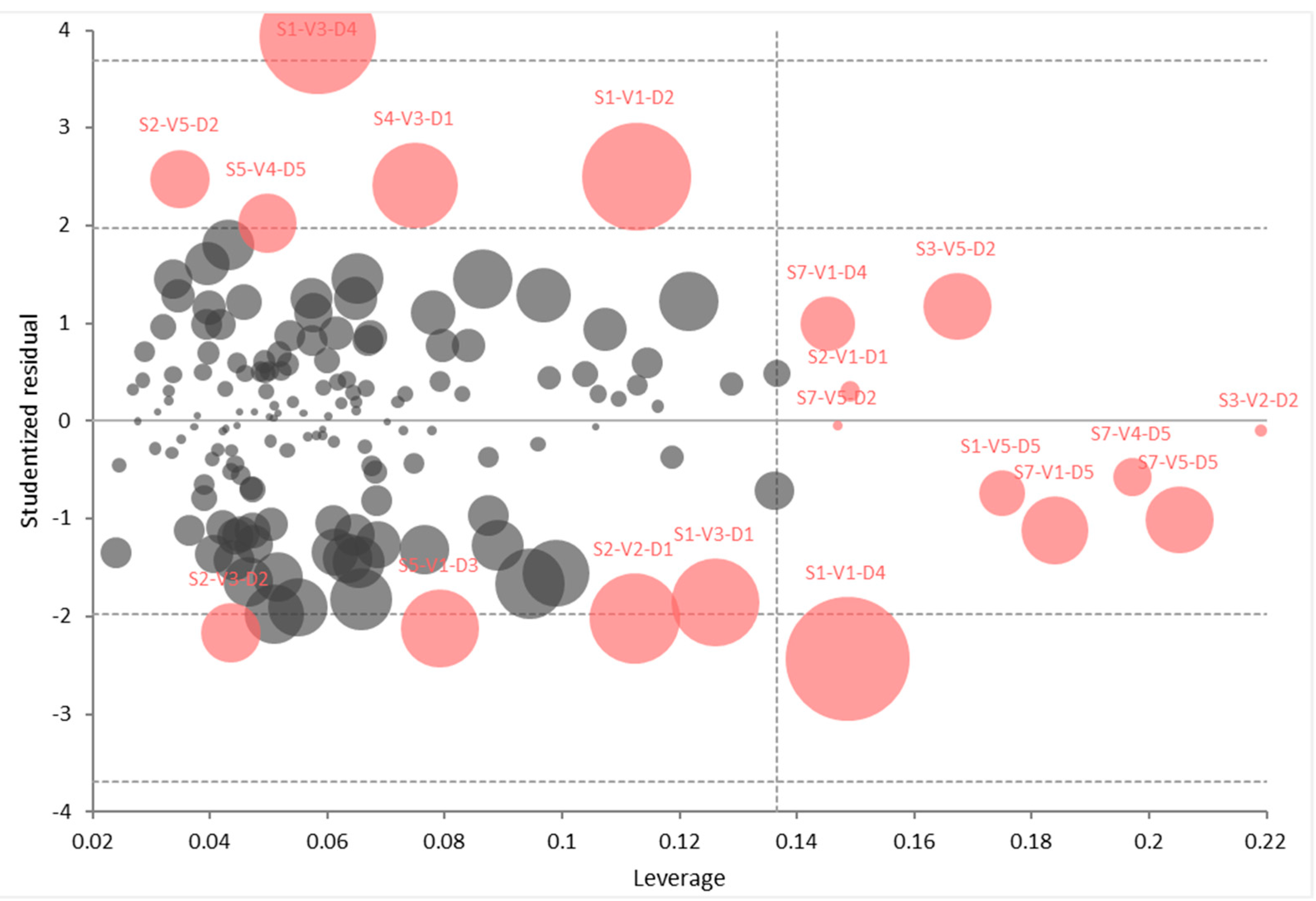
Finally, Figure 8 presents the leverage and influence of sampling points on the fitted model. The size of each sampling point is the square root of Cook’s D statistic (a measure of the influence of the sampling point). Data outliers can be considered as points with a large residual (usually +/−2), while the points with high leverage are plotted to the right of the diagram. It should be noted that data points with a significant residual and high leverage had the most influence on the fitted model.
During the regression analysis, a total of four data points (167 data points in total) were omitted from the computation due to their extremely high leverage, namely S3-V5-D4, S3-V5-D5, S3-V3-D3, and S1-V3-D2.
Although the correlation coefficient of the model given by Equation (6) indicated only a moderate correlation with the measured results, it can be stated that pH, electric conductivity, some of the macronutrients as well as the presence of organic matter (represented by BOD and COD) do influence the values of chlorophyll-a. This conclusion is supported by the fact that the model itself is statistically significant (F-test) despite the relatively low value of the correlation coefficient.
Another water quality parameter for which a model was developed using the principles of multivariate analysis was dissolved oxygen. The predictor parameters were chlorophyll-a, water temperature, pH, and depth. Chlorophyll-a was selected due to the fact that photosynthesis generates oxygen. Water temperature was chosen since the solubility of oxygen decreases as water temperature increases. On the other hand, photosynthesis depletes carbonate, which can produce a significant increase in pH at constant alkalinity. Hence pH was also taken as a possible predictor of dissolved oxygen. Finally, depth was also considered. The reason for the latter is that depth could be used as a substitution for other parameters that can influence dissolved oxygen levels and were not measured during the data collection campaign. One of these parameters is reaeration, which has to have higher values at low depths, etc. The selection of the predictor parameters was supported by research conducted by other authors [31]. The parameters’ 2nd, 3rd, and 4th polynomials were also included in the analysis along with their full interaction terms (in this case, up to 4-way interactions). Stepwise regression was used to select the terms to be used in the final model. The following fitted equation (model) was attained
The acquired equation had a correlation coefficient of 0.872, i.e., a strong correlation to the measured results. Using the F-test, it was also computed that Equation (7) was better than the null model at the 5% significance level (since its -value was <0.0001). The analysis also yielded -values that confirmed that all the terms in Equation (7) contribute to the model at the 5% significance level. The effect of the fitted model is given in Figure 9.
As in the case of the fitted model for Chlorophyll-a, all the necessary subsequent analyses were conducted. However, here, only the results will be reported without graphical presentation to avoid unnecessary cluttering of results.
The Shapiro–Wilk normality test confirmed that the fitted model’s residuals followed the normal distribution at the 5% significance level. The leverage and influence of sampling points were also analyzed. During the conducted regression analysis, a total of three data points (167 data points in total) were omitted from the analysis due to their extremely high leverage, namely S7-V5-D1, S4-V3-D1, and S1-V3-D4.
Both the strong correlation between Equation (6) and the measured results and the developed model’s statistical significance (F-test) indicated that water temperature, pH, chlorophyll-a, and depth have a meaningful influence on the dissolved oxygen values. It should be noted that depth most probably has an indirect effect through its correlation with other parameters that were not measured, such as reaeration.
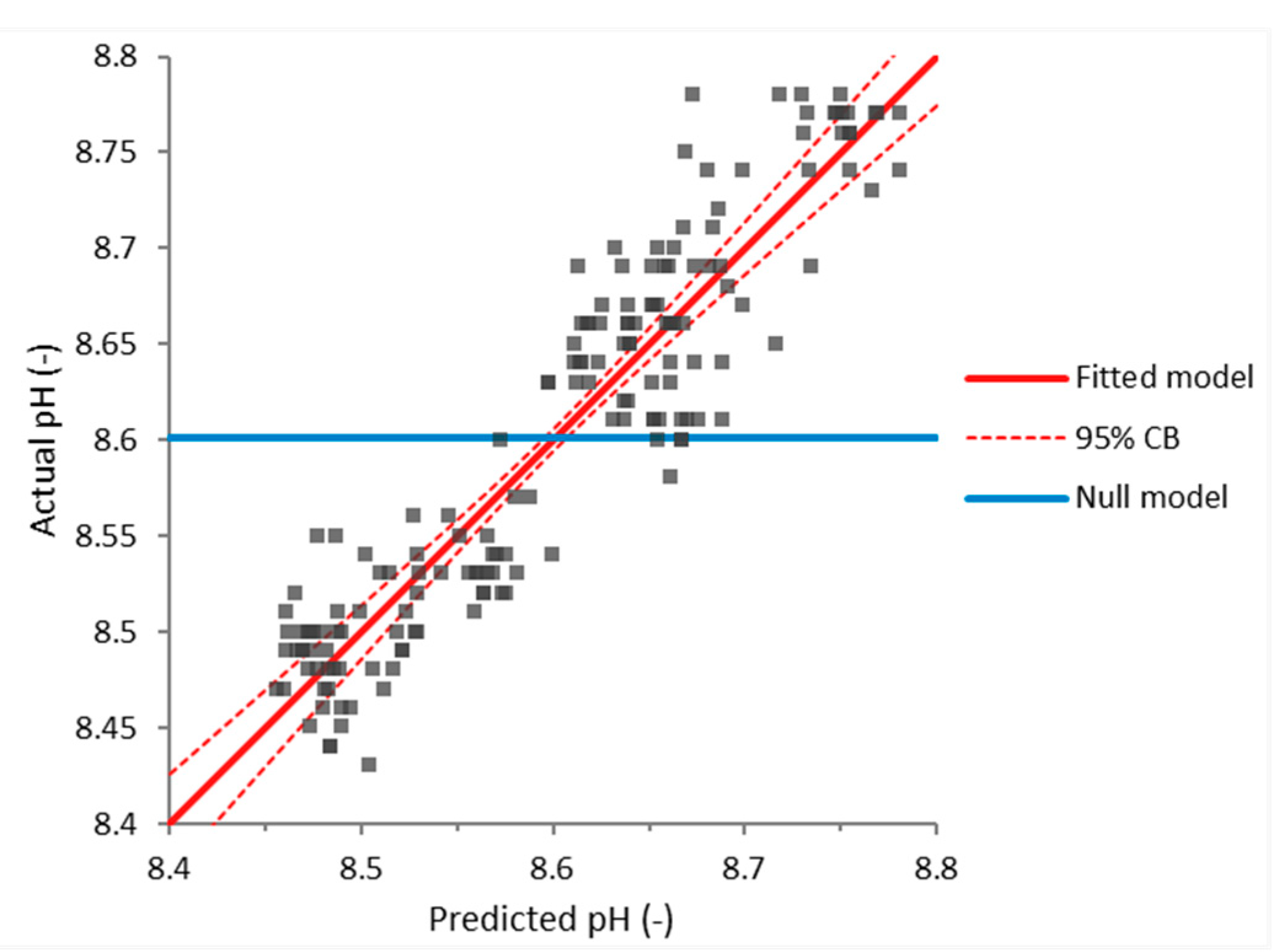
The final water quality parameter, for which a model was developed using the principles of multivariate analysis, was pH. Naturally, the selection of the predictor parameters was supported by research conducted by other authors [31]. The predictor parameters were dissolved oxygen and water temperature. The parameters’ 2nd, 3rd, and 4th polynomials were also included in the analysis along with their full interaction terms (in this case, up to 2-way interactions). Stepwise regression was used to select the terms to be used in the final model. The following fitted equation (model) was attained
The acquired equation had a correlation coefficient of 0.866, i.e., a strong correlation to the measured results. Using the F-test, it was also computed that Equation (7) was better than the null model at the 5% significance level (since its p-value was <0.0001). The analysis also yielded p-values that confirmed that all the terms in Equation (8) contributed to the model at the 5% significance level. The effect of the fitted model is given in Figure 10.
Both the strong correlation between Equation (7) and the measured results and the developed model’s statistical significance (F-test) indicated that water temperature and pH influence pH levels considerably. It should be noted that this conclusion is in accordance with results published by other authors [31,32].
4. Conclusions
On the Danube reach between Hungary and Serbia (RKM 1438 and RKM 1432), water quality measurements were conducted in 2011. Seven data ranges (cross-sections) were analyzed. Every cross-section contained five verticals with five sampling points distributed over the water depth. Twelve water quality parameters were monitored: water temperature, dissolved oxygen, different forms of nitrogen and phosphorous, turbidity, organic pollution, and the presence of algae (chlorophyll-a). Several multivariate analysis tools were used to analyze the gathered data set, including the principal component analysis.
The conducted analysis confirmed no significant correlation between the water depth and the monitored water quality parameters. This is the consequence of vertical mixing due to turbulent diffusion. This phenomenon is intense enough to prevent any stratification that would facilitate different chemical and/or biological processes at different water depths. Hence, the depth plays virtually no role in collecting representative samples for a given cross-section of the analyzed watercourse.
As to the position of the sampling location with respect to the width of the cross-section, i.e., the sampling location’s lateral position, the performed analysis did not give unambiguous results. Generally speaking, there was a detectable clustering of sampling points within specific verticals in some cross-sections. In other cross-sections, this kind of clustering was very mild. However, it can be concluded that taking water quality samples from the middle of the flow should give descriptive results of that particular cross-section.
The principal component analysis conducted for the entire analyzed river reach clearly showed clustering of sampling points with respect to their cross-sections. Although this observation could be the consequence of the unsteady flow in rivers, additional considerations point to the fact that the position of a cross-section can have a significant impact on the measured water quality parameters, i.e., the cross-section’s spatial offset affects the water quality parameters.
Using the gathered data, a fitted equation (model) was developed for predicting chlorophyll-a. All the measured water quality parameters were initially selected, their 2nd order terms, as well as 2-way interactions for every term pair. Then, stepwise regression was used to select the terms to be used in the final equation. The model’s correlation coefficient with respect to the measured values was moderate (0.43), although the F-test indicates that the model was statistically significant. Fitted equations were also developed for dissolved oxygen and pH prediction. For both models, the F-test indicated that they were statistically significant, while the correlation coefficients indicated a strong correlation (0.872 for DO and 0.866 for pH) with the measured values for both models.
However, it should also be noted that the fitted models presented here cannot be used as a general-purpose tool. Instead, they merely serve as examples of how to use regression analysis when dealing with water quality analysis in alluvial rivers.
The overall methodology for analyzing water quality parameters presented in this paper gives a reasonable basis for further research concerning biological and/or chemical processes in alluvial watercourses.
Author Contributions
Conceptualization, Z.H. and M.H.; methodology, Z.H. and M.H.; software, Z.H. and K.P.; validation, V.B., and N.P.; formal analysis, K.P.; investigation, Z.H.; resources, M.H.; data curation, N.P.; writing—original draft preparation, M.H. and K.P.; writing—review and editing, K.P. and N.P.; visualization, Z.H.; supervision, Z.H.; project administration, K.P.; funding acquisition, Z.H. All authors have read and agreed to the published version of the manuscript.
Funding
This work was supported by the Ministry of Education, Science and Technological Development of the Republic of Serbia (program no. 451-03-9/2021-14/200093 and 451-03-9/2021-14/200134).
Institutional Review Board Statement
Not applicable.
Informed Consent Statement
Not applicable.
Data Availability Statement
All data generated or analyzed during this study are available from the corresponding author on reasonable request.
Conflicts of Interest
The authors declare no conflict of interest.
References
- Ji, Z.-G. Hydrodynamics and Water Quality: Modeling Rivers, Lakes, and Estuaries, 2nd ed.; John Wiley & Sons: Hoboken, NJ, USA, 2009; pp. 247–336. [Google Scholar]
- Mohamed, I.; Othman, F.N.; Ibrahim, A.I.; Alaa-Eldin, M.E.; Yunus, R.M. Assessment of water quality parameters using multivariate analysis for Klang River basin. Malaysia. Environ. Monit. Assess. 2014, 187, 4182. [Google Scholar] [CrossRef] [PubMed]
- Yilma, M.; Kiflie, Z.; Gessese, N. Assessment and interpretation of river water quality in Little Akaki River using multivariate statistical techniques. Int. J. Environ. Sci. Technol. 2019, 16, 3707–3720. [Google Scholar] [CrossRef]
- Horvat, M.; Horvat, Z. Implementation of a monitoring approach: The Palic-Ludas lake system in the Republic of Serbia. Environ. Monit. Assess. 2020, 192, 150. [Google Scholar] [CrossRef] [PubMed]
- Kumari, R.; Sharma, R.C. Assessment of water quality index and multivariate analysis of high altitude sacred Lake Prashar, Himachal Pradesh, India. Int. J. Environ. Sci. Technol. 2019, 16, 6125–6134. [Google Scholar] [CrossRef]
- Satheeshkumar, P.; Khan, A.B. Identification of mangrove water quality by multivariate statistical analysis methods in Pondicherry coast, India. Environ. Monit. Assess. 2012, 184, 3761–3774. [Google Scholar] [CrossRef] [PubMed] [Green Version]
- Horvat, M.; Horvat, Z.; Pastor, K. Multivariate analysis of water quality parameters in Lake Palic, Serbia. Environ. Monit. Assess. 2021, 193, 410. [Google Scholar] [CrossRef]
- Horvat, Z.; Isic, M.; Spasojevic, M. Two dimensional river flow and sediment transport model. Environ. Fluid Mech. 2015, 15, 595–625. [Google Scholar] [CrossRef]
- Horvat, Z.; Horvat, M. Two dimensional heavy metal transport model for natural watercourses. River Res. Appl. 2016, 32, 1327–1341. [Google Scholar] [CrossRef]
- Horvat, Z.; Horvat, M.; Koch, D.; Majer, F. Field measurements on alluvial watercourses in light of numerical modeling: Case studies on the Danube River. Environ. Monit. Assess. 2021, 193, 6. [Google Scholar] [CrossRef]
- Cozzolino, D.; Power, A.; Chapman, J. Interpreting and Reporting Principal Component Analysis in Food Science Analysis and Beyond. Food Anal. Methods 2019, 12, 2469–2473. [Google Scholar] [CrossRef]
- Bro, R.; Smilde, A.K. Principal component analysis: A tutorial review. Anal. Methods 2014, 6, 2812–2831. [Google Scholar] [CrossRef] [Green Version]
- Vandeginste, B.G.M.; Massart, D.L.; Buydens, L.M.C.; Jong, S.D.E.; Lewi, P.J.; Smeyers-Verbeke, J. Handbook of Chemometrics and Qualimetrics: Part B; Elsevier: Amsterdam, The Netherlands, 1998. [Google Scholar]
- Bengräine, K.; Marhaba, T.F. Using principal component analysis to monitor spatial and temporal changes in water quality. J. Hazard. Mater. 2003, 100, 179–195. [Google Scholar] [CrossRef]
- Ouyang, Y. Evaluation of river water quality monitoring stations by principal component analysis. Water Res. 2005, 39, 2621–2635. [Google Scholar] [CrossRef]
- Helena, B.; Pardo, R.; Vega, M.; Barrado, E.; Fernandez, J.M.; Fernandez, L. Temporal evolution of groundwater composition in an alluvial aquifer (Pisuerga River, Spain) by principal component analysis. Water Res. 2000, 34, 807–816. [Google Scholar] [CrossRef]
- Yan, J.; Liu, J.; Yu, Y.; Xu, H. Water Quality Prediction in the Luan River Based on 1-DRCNN and BiGRU Hybrid Neural Network Model. Water 2021, 13, 1273. [Google Scholar] [CrossRef]
- Lim, J.-S.; Kim, Y.-W.; Lee, J.-H.; Park, T.-J. Evaluation of correlation between chlorophyll-a and multiple parameters by multiple linear regression analysis. J. Korean Soc. Environ. Eng. 2015, 37, 253–261. [Google Scholar] [CrossRef]
- Li, X.; Sha, J.; Wang, Z.-L. A comparative study of multiple linear regression, artificial neural network and support vector machine for the prediction of dissolved oxygen. Hydrol. Res. 2017, 48, 1214–1225. [Google Scholar] [CrossRef]
- Clesceri, L.S.; Greenberg, A.E.; Eaton, A.D. (Eds.) Standard Methods for the Examination of Water and Wastewater, 20th ed.; American Public Health Association (APHA): Washington, DC, USA; The American Water Works Association (AWWA): Washington, DC, USA; The Water Environment Federation (WEF): Washington, DC, USA, 1999. [Google Scholar]
- Čoha, F. Voda za piće-Standardne metode za ispitivanje higijenske ipravnosti. In NIP Privredni Pregled; Savezni Zavod za Zdravstvenu Zaštitu: Beograd, Srbija, 1990. (In Serbian) [Google Scholar]
- Shapiro, S.S.; Wilk, M.B. An analysis of variance test for normality (complete samples). Biometrika 1965, 52, 591–611. [Google Scholar] [CrossRef]
- Box, G.E.P. Non-Normality and Tests on Variances. Biometrika 1953, 40, 318–335. [Google Scholar] [CrossRef]
- Vaccari, D.A.; Wang, H.-K. Multivariate polynomial regression for identification of chaotic time series. Math. Comput. Model. Dyn. Syst. 2007, 13, 395–412. [Google Scholar] [CrossRef]
- Sinha, P. Multivariate polynomial regression in data mining: Methodology, problems and solutions. Int. J. Sci. Eng. Res. 2013, 4, 962–965. [Google Scholar]
- Petersen, W.; Bertino, L.; Callies, U.; Zorita, E. Process identification by principal component analysis of river water-quality data. Ecol. Modell. 2001, 138, 193–213. [Google Scholar] [CrossRef]
- Debska, K.; Rutkowska, B.; Szulc, W.; Gozdowski, D. Changes in Selected Water Quality Parameters in the Utrata River as a Function of Catchment Area Land Use. Water 2021, 13, 2989. [Google Scholar] [CrossRef]
- Lorenz, M.; Nguyen, H.Q.; Le, T.D.H.; Zeunert, S.; Dang, D.H.; Le, Q.D.; Le, H.; Meon, G. Discovering Water Quality Changes and Patterns of the Endangered Thi Vai Estuary in Southern Vietnam through Trend and Multivariate Analysis. Water 2021, 13, 1330. [Google Scholar] [CrossRef]
- Maiolo, M.; Pantusa, D. Multivariate Analysis of Water Quality Data for Drinking Water Supply Systems. Water 2021, 13, 1766. [Google Scholar] [CrossRef]
- Li, S.; Wang, Y.; Liu, L.; Lai, H.; Zeng, X.; Chen, J.; Liu, C.; Luo, Q. Temporal and Spatial Distribution of Microplastics in a Coastal Region of the Pearl River Estuary, China. Water 2021, 13, 1618. [Google Scholar] [CrossRef]
- Heddam, S.; Kisi, O. Modelling daily dissolved oxygen concentration using least square support vector machine, multiple adaptive regression splines and M5 model tree. J. Hydrol. 2018, 559, 499–509. [Google Scholar] [CrossRef]
- Pestorić, B.; Drakulović, D.; Gvozdenović, S. Composition of microbiology, phytoplankton and bio-toxins in water and mussel on fish and shellfish farms in Boka Kotorska bay (Se Adriatic Sea). J. Agron. Technol. Eng. Manag. 2019, 2, 207–217. [Google Scholar]
Figure 1.
Placement of the data ranges and their verticals within the analyzed river reach.
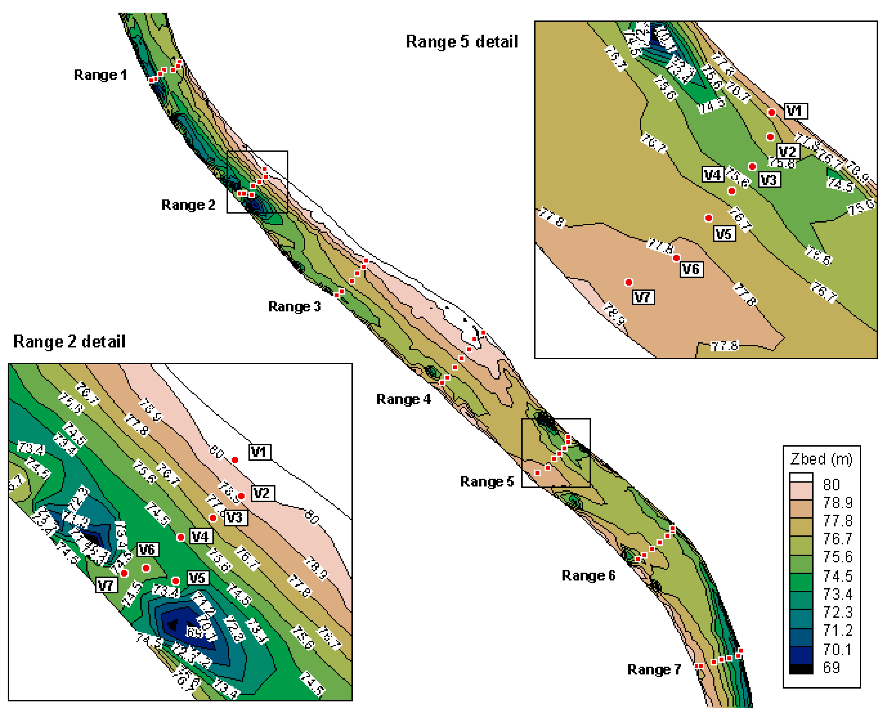
Figure 2.
Box plots of the measured water quality measurements.
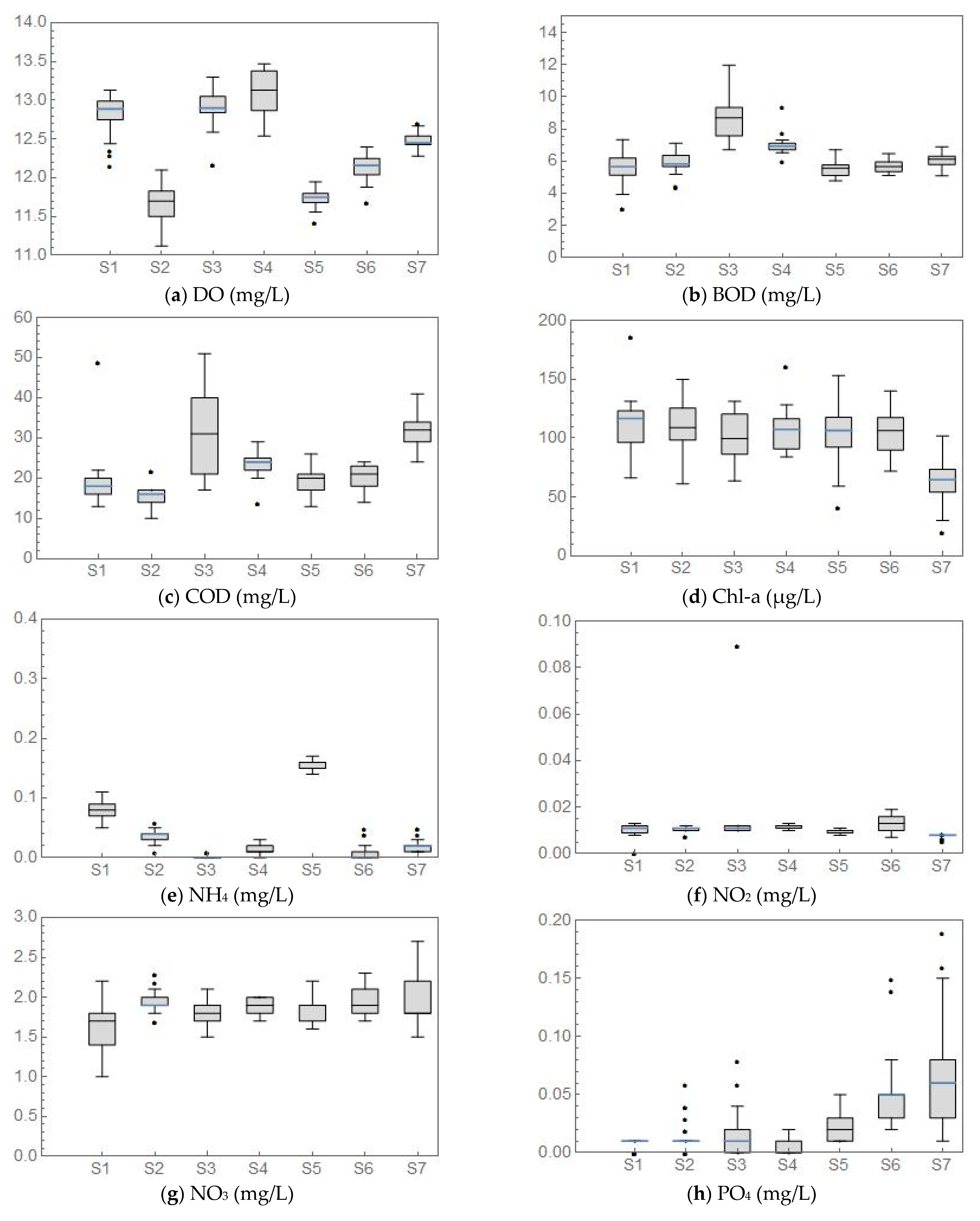
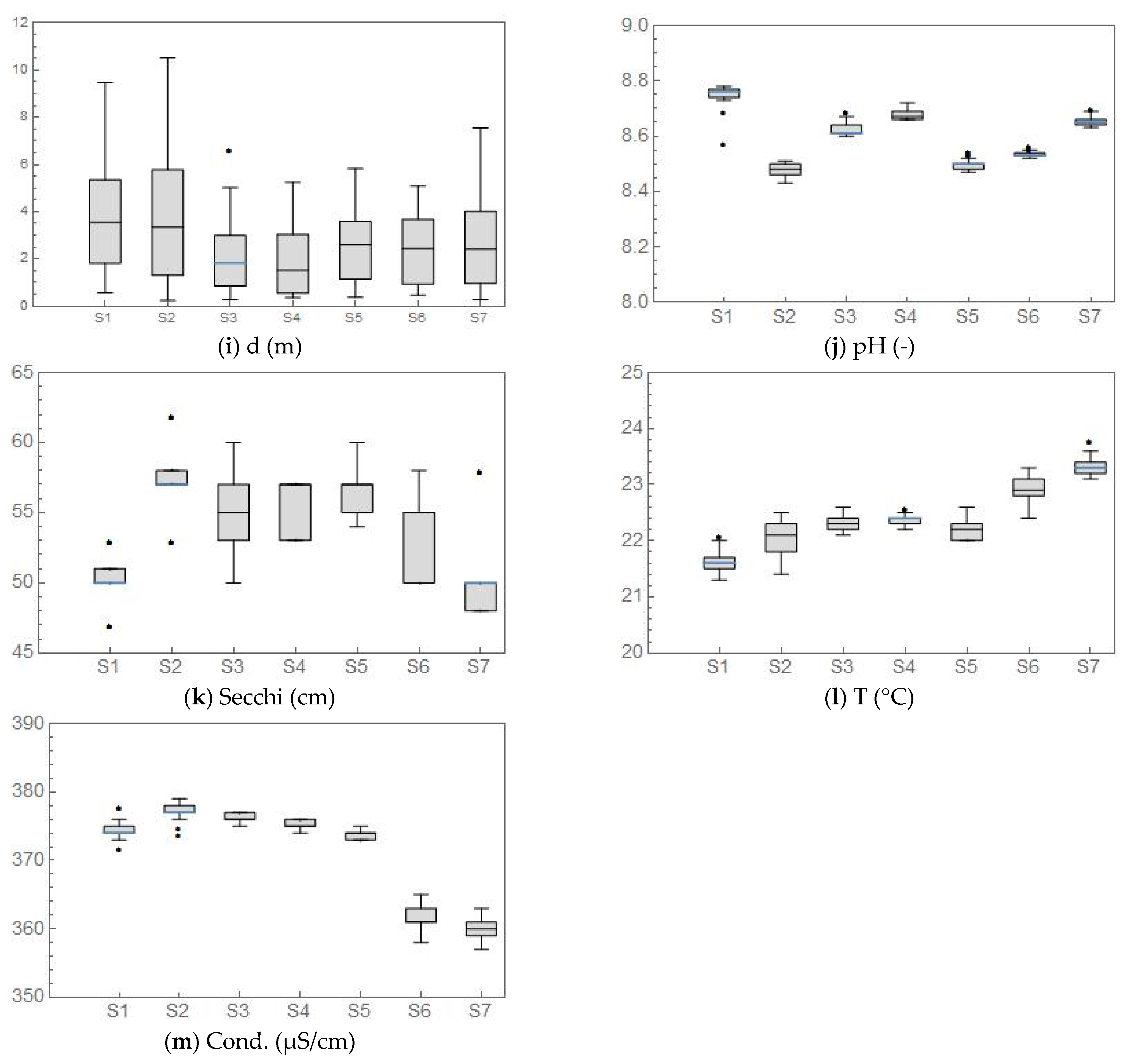
Figure 3.
Normality (Shapiro–Wilk) test results for Chlorophyll-a.

Figure 4.
PCA results for each cross-section (data range) of the analyzed river reach.
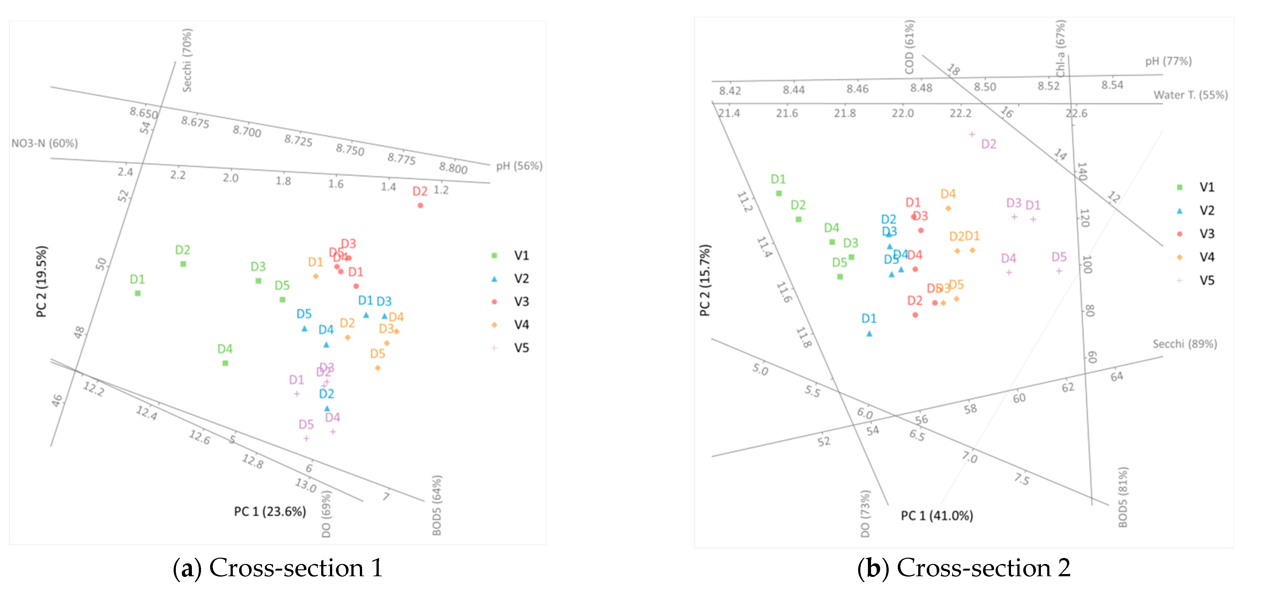
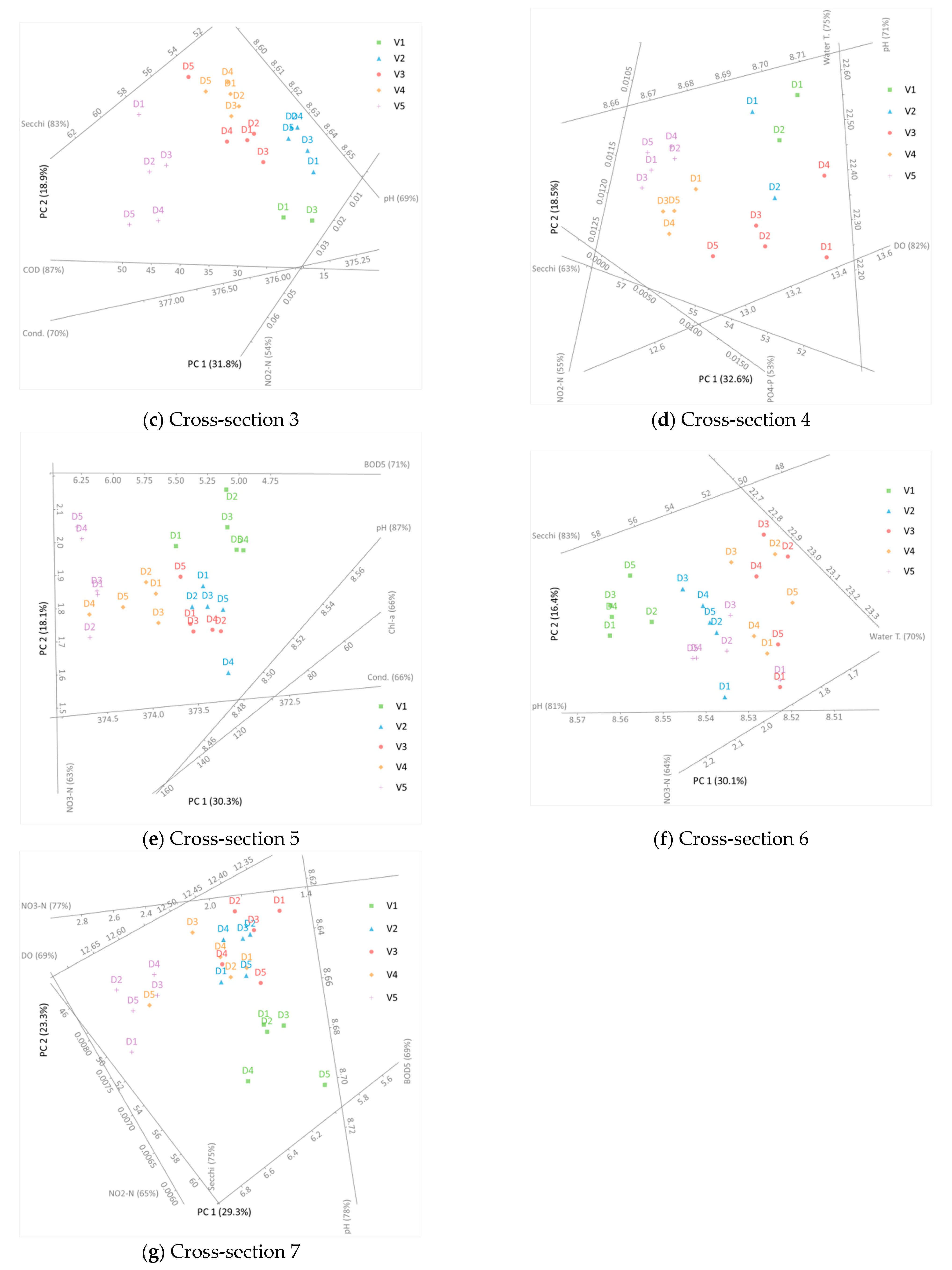
Figure 5.
PCA results for the entire analyzed river reach.

Figure 6.
Effect of the fitted model (predicted and actual values) for Chl-a.
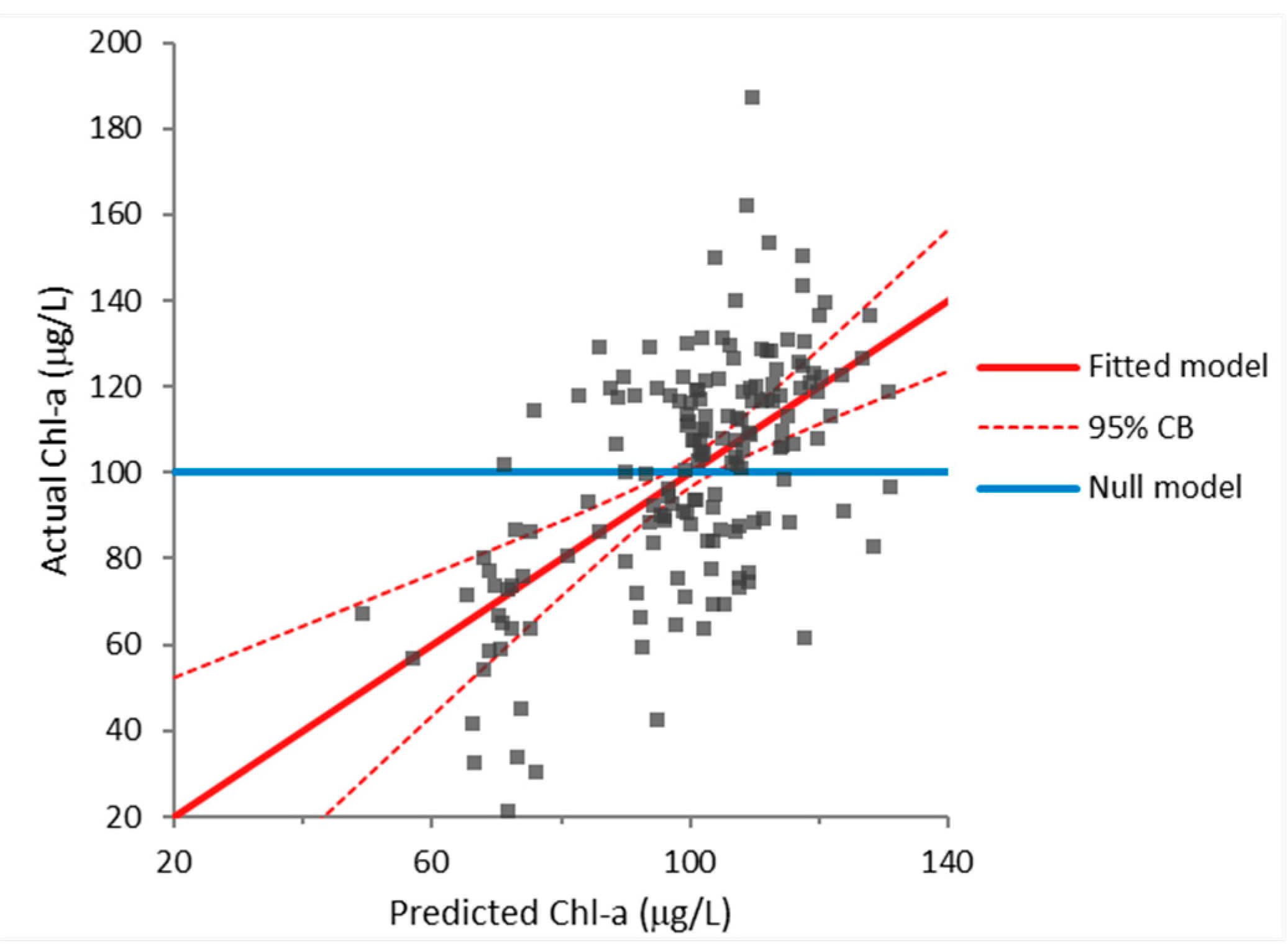
Figure 7.
Analysis of the fitted model’s residuals for Chl-a. (a) Fitted model’s residuals. (b) Frequency plot of the fitted model’s residuals. (c) Residuals plotted against a normal theoretical quantile.
Figure 7.
Analysis of the fitted model’s residuals for Chl-a. (a) Fitted model’s residuals. (b) Frequency plot of the fitted model’s residuals. (c) Residuals plotted against a normal theoretical quantile.
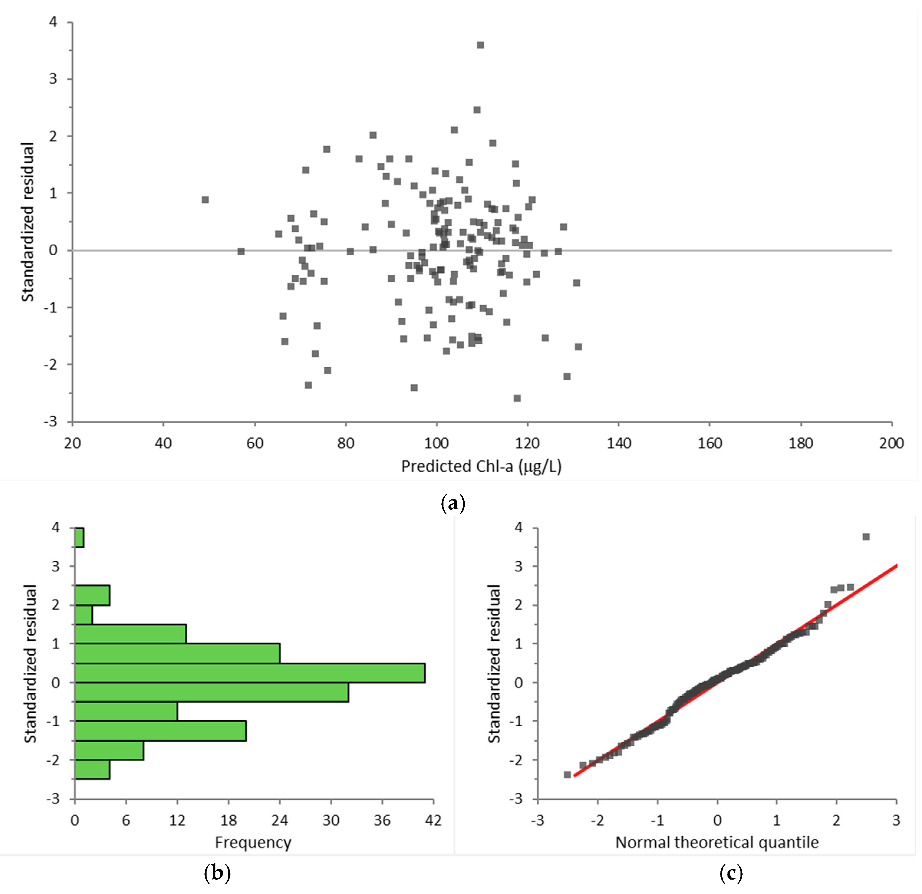
Figure 8.
Outliers, leverage, and influence of sampling points on the fitted model for Chl-a.

Figure 9.
Effect of the fitted model (predicted and actual values) for DO.
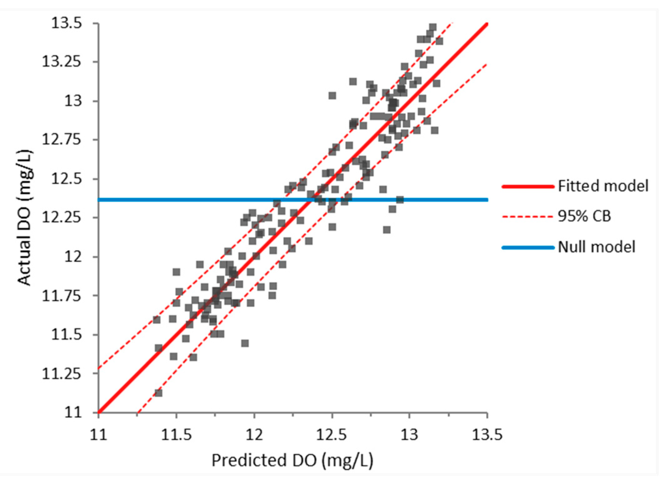
Figure 10.
Effect of the fitted model (predicted and actual values) for pH.

Table 1.
Names, locations, and sampling times for the data ranges.
| Cross-Section | rkm | Date of Measurement |
|---|---|---|
| 1 | 1438 | 23 May 2011 |
| 2 | 1437 | 24 May 2011 |
| 3 | 1436 | 24 May 2011 |
| 4 | 1435 | 24 May 2011 |
| 5 | 1434 | 25 May 2011 |
| 6 | 1433 | 27 May 2011 |
| 7 | 1432 | 27 May 2011 |
Table 2.
Methods used for determining water quality parameters.
| Parameter | Method |
|---|---|
| Water temperature | 2250B * |
| pH | 500-H+B * |
| Electric conductivity | SRPS EN 27888/2009 |
| Dissolved oxygen | SRPS EN 25813:2009/1/2011 |
| Orthophosphates | SRPS EN ISO 6878:2008 |
| Nitrite nitrogen | SRPS EN 26777:2009 |
| Nitrate nitrogen | SRPS EN ISO 10304-1:2009 |
| Ammonia nitrogen | ** |
| Chemical oxygen demand | EPA 410.4 US 5220D, ISO 15705 |
| Biochemical oxygen demand | SRPS EN 1899-1:2009 |
| Chlorophyll-a | 10200-H * |
Table 3.
Correlation coefficients between the measured water quality parameters.
| d | T | pH | Cond | DO | NO2 | NO3 | NH4 | PO4 | COD | Chl-a | BOD | Secchi | |
|---|---|---|---|---|---|---|---|---|---|---|---|---|---|
| d | - | ||||||||||||
| T | −0.008 | - | |||||||||||
| pH | −0.006 | −0.097 | - | ||||||||||
| Cond | 0.071 | −0.815 | −0.04 | - | |||||||||
| DO | −0.173 | −0.027 | 0.838 | 0.044 | - | ||||||||
| NO2 | −0.107 | −0.015 | −0.024 | 0.122 | 0.086 | - | |||||||
| NO3 | −0.144 | 0.351 | −0.283 | −0.229 | −0.208 | −0.046 | - | ||||||
| NH4 | 0.059 | −0.413 | −0.177 | 0.298 | −0.402 | −0.149 | −0.123 | - | |||||
| PO4 | −0.067 | 0.583 | −0.092 | −0.62 | −0.097 | −0.056 | 0.248 | −0.193 | - | ||||
| COD | −0.115 | 0.416 | 0.28 | −0.289 | 0.364 | 0.293 | 0.032 | −0.333 | 0.303 | - | |||
| Chl-a | 0.069 | −0.426 | −0.11 | 0.444 | −0.046 | 0.147 | −0.19 | 0.143 | −0.294 | −0.297 | - | ||
| BOD | −0.106 | 0.072 | 0.187 | 0.246 | 0.51 | 0.306 | −0.102 | −0.409 | −0.126 | 0.36 | 0.092 | - | |
| Secchi | 0.113 | −0.079 | −0.468 | 0.358 | −0.373 | 0.163 | 0.026 | 0.116 | −0.251 | −0.085 | 0.149 | 0.126 | - |
Table 4.
Percentage of the original data’s variation contained in the first two principal components.
Table 4.
Percentage of the original data’s variation contained in the first two principal components.
| Cross-Section | Variation % |
|---|---|
| S1 | 43.2 |
| S2 | 56.6 |
| S3 | 50.7 |
| S4 | 51.2 |
| S5 | 48.4 |
| S6 | 46.5 |
| S7 | 52.6 |
Publisher’s Note: MDPI stays neutral with regard to jurisdictional claims in published maps and institutional affiliations. |
© 2021 by the authors. Licensee MDPI, Basel, Switzerland. This article is an open access article distributed under the terms and conditions of the Creative Commons Attribution (CC BY) license (https://creativecommons.org/licenses/by/4.0/).
Share and Cite
MDPI and ACS Style
Horvat, Z.; Horvat, M.; Pastor, K.; Bursić, V.; Puvača, N. Multivariate Analysis of Water Quality Measurements on the Danube River. Water 2021, 13, 3634. https://doi.org/10.3390/w13243634
AMA Style
Horvat Z, Horvat M, Pastor K, Bursić V, Puvača N. Multivariate Analysis of Water Quality Measurements on the Danube River. Water. 2021; 13(24):3634. https://doi.org/10.3390/w13243634
Chicago/Turabian StyleHorvat, Zoltan, Mirjana Horvat, Kristian Pastor, Vojislava Bursić, and Nikola Puvača. 2021. "Multivariate Analysis of Water Quality Measurements on the Danube River" Water 13, no. 24: 3634. https://doi.org/10.3390/w13243634
Note that from the first issue of 2016, this journal uses article numbers instead of page numbers. See further details here.