Article

Splitting and Length of Years for Improving Tree-Based Models to Predict Reference Crop Evapotranspiration in the Humid Regions of China

1
Key Laboratory of Agricultural Soil and Water Engineering in Arid and Semiarid Areas of the Ministry of Education, Northwest A&F University, Yangling, Xianyang 712100, China
2
School of Hydraulic and Ecological Engineering, Nanchang Institute of Technology, Nanchang 330099, China
3
State Key Laboratory of Simulation and Regulation of Water Cycle in River Basin, China Institute of Water Resources and Hydropower Research, Beijing 100038, China
*
Authors to whom correspondence should be addressed.
Water 2021, 13(23), 3478; https://doi.org/10.3390/w13233478
Submission received: 1 November 2021 / Revised: 23 November 2021 / Accepted: 24 November 2021 / Published: 6 December 2021
(This article belongs to the Section Hydrology)

Abstract

:
To improve the accuracy of estimating reference crop evapotranspiration for the efficient management of water resources and the optimal design of irrigation scheduling, the drawback of the traditional FAO-56 Penman–Monteith method requiring complete meteorological input variables needs to be overcome. This study evaluates the effects of using five data splitting strategies and three different time lengths of input datasets on predicting ET0. The random forest (RF) and extreme gradient boosting (XGB) models coupled with a K-fold cross-validation approach were applied to accomplish this objective. The results showed that the accuracy of the RF (R2 = 0.862, RMSE = 0.528, MAE = 0.383, NSE = 0.854) was overall better than that of XGB (R2 = 0.867, RMSE = 0.517, MAE = 0.377, NSE = 0.860) in different input parameters. Both the RF and XGB models with the combination of Tmax, Tmin, and Rs as inputs provided better accuracy on daily ET0 estimation than the corresponding models with other input combinations. Among all the data splitting strategies, S5 (with a 9:1 proportion) showed the optimal performance. Compared with the length of 30 years, the estimation accuracy of the 50-year length with limited data was reduced, while the length of meteorological data of 10 years improved the accuracy in southern China. Nevertheless, the performance of the 10-year data was the worst among the three time spans when considering the independent test. Therefore, to improve the daily ET0 predicting performance of the tree-based models in humid regions of China, the random forest model with datasets of 30 years and the 9:1 data splitting strategy is recommended.

1. Introduction

Evapotranspiration (ET), the total water consumption of soil evaporation and crop transpiration, is of great significance for water resources planning and management, irrigation systems, land drainage implementation, groundwater research, drought assessment, analysis of farmland environments, and agricultural water management in water shortage areas [1,2,3,4]. The precise prediction of ET is critical at the global level because it has an impact on the hydrological cycle [5,6]. In the context of climate change, agricultural water resources are decreasing on a temporal and spatial scale across the world [7]. Crop water use is the key factor of soil water circulation in farmland, which is exceedingly significant regarding the optimal allocation of water resources and the formulation of irrigation systems, and the key to calculate the crop water demand is to determine the evapotranspiration of crops [8,9,10]. However, methods for calculating the ET, such as the water balance method [11], the conduction theory of aqueous vapor [12], or using the lysimeter device, are extremely time-consuming and expensive in practice, which limits their applicability. Hence, to determine the actual ET value in a wide range, the reference evapotranspiration (ET0) was developed as an alternative method for calculating the ET and has been widely used [13].
Plenty of nonlinear mathematical models with meteorological variables have been established for ET0 prediction [14,15,16], among which the FAO-56 Penman–Monteith model is the most widely accepted standard model in different regions and climates. However, the FAO-56 Penman–Monteith model needs a mass of meteorological variables for its calculation, e.g., maximum and minimum ambient temperatures, wind speed, relative humidity, and solar radiation [17,18,19], which is the major weaknesses for its application across the world. Therefore, models with fewer meteorological parameters as inputs, e.g., temperature-based, mass transfer-based, and radiation-based models, have been developed and applied widely in regions where only incomplete meteorological data are available [6,20,21,22,23]. In spite of the wide application, there are still many inconveniences in the estimation of evapotranspiration with empirical models as most of them are linear functions, while evapotranspiration in reality is a highly complicated nonlinear process.
Over the past few decades, machine learning models have been successfully modeled in various fields (i.e., pan evaporation, dew point temperature, global solar radiation, streamflow, water quality, drought events, etc.) due to their excellence in dealing with complex and nonlinear relationships [23,24,25,26,27,28,29,30,31,32,33,34,35,36,37,38,39], including in the field of ET0 estimation [40,41]. For example, various algorithms, including artificial neural networks [42,43,44], extreme learning machines [45,46,47], support vector machines [48,49,50], gene expression programming [51,52,53], extreme gradient boosting [54,55,56], M5 model tree [57,58], and deep learning [59,60,61], have been evaluated for their capability in estimating the ET0.
The random forest (RF) is an ensemble-based method. Due to the random forest being able to handle extremely large datasets, RF has been commonly used for predicting ET0 in recent years [62,63,64,65]. For example, Feng et al. studied the capabilities of the RF and GRNN models for estimating the daily ET0 with meteorological parameters from two weather stations in southwest China and discovered that both RF and GRNN performed well, while RF was a little better than GRNN in general [62]. Wang et al. reported that the derived generalized ET0 model based on the RF could be successfully applied to ET0 estimation with both complete and incomplete meteorological variables, which was recommended for application in water balance research [65]. Junior et al. predicted ET0 with the inverse distance weighting (IDW), ordinary kriging (OK), random forest (RF), and a random forest variation for spatial predictions (RFsp) based on maximum and minimum temperature data from 136 climatological stations located in Brazil, in which they found that the RF obtained better results than conventional approaches [63]. Karimi et al. used 10-year daily data from Iran and considered the impact of replacing missing meteorological variables with calculated meteorological variables based on the standard FAO-56 PM, some commonly used empirical equations, and the random forest model [5]. According to their results, when the calculated value was used to replace the missing variable, the RF model based on the combination of wind speed has higher accuracy than the RF model based on the combination of solar radiation. In addition, the random forest was also widely used in flood probability mapping [65,66], and there are relevant reports using remote sensing data [67,68]. Meanwhile, the random forest has also been well applied in water quality [69].
In recent years, because the error is reduced, the prediction accuracy is better and the calculation costs are lower. Chen and Guestrin proposed the tree-based extreme gradient boosting (XGB) [70], which has been widely applied in various fields [71,72,73]. In addition, the model has also been used to predict ET0. For example, Wu et al. explored the performance of the XGB model in estimating the monthly mean daily ET0 using temperature data and found that the XGB model exhibited better estimation accuracy than the other methods [74]. Fan et al. evaluated the capability of the XGB model in estimating daily reference evapotranspiration using the Global Ensemble Reforecast v2 data in different climatic zones of China [75]. The results indicated that the XGB model can be satisfactory for estimating the daily ET0. Furthermore, the optimization algorithm of the XGB model has received more and more attention because of its ability to enhance the ability of artificial intelligence methods in the modeling process of solving engineering problems, and it has been used to estimate ET0 [76,77,78]. Therefore, the XGB model is suited to estimate the daily ET0 in data-limited regions.
Machine learning models of different heuristic agrometeorological variables have shown high accuracy in ET0 estimation based on finite data. However, the soundness of the model to overcome the complexity in reality and to obtain high-precision simulating results is highly dependent on the data management strategy during model development and evaluation, especially for the splitting strategy of data allocating to the model training and testing stages. Therefore, the key to ensuring a model obtaining the best simulation accuracy with the data series is to find a suitable standard for appropriately splitting the data into the model training and testing stages. For instance, Wu et al. established an RF model with a 2:1 data splitting for the training and testing and found that the RF had higher simulation accuracy than the other intelligent models [74]. To find an alternative method of mass transfer-based methods, Shiri et al. established a random forest using a cross-validation at the local and cross-station scales with a single data splitting for the training and testing series [79]. It was found that the simulation accuracy of the random forest model was better than the transfer-based models.
In the context of climate change, both meteorological factors and ET0 have changed a great deal [80,81]. This poses a challenge to model establishment and evaluation for estimation with a long-term period of data, and the efficiency for the model estimating ET0 is related to the time length of the input datasets [4,82,83,84]. Yassen et al. divided a 35-year historical record (1983–2017) into four groups (i.e., 17 years (long-term), 10 years and 7 years (middle-term), and 5 years (short-term)) to study the temporal and spatial changes of Egypt’s annual reference evapotranspiration [85]. The results indicated that the short-term group showed the most significant differences in all the studied areas of Egypt, while the long-term and medium-term differences were only significantly different in a certain area of Egypt. Ning et al. studied the interaction of the three factors (i.e., vegetation, climate, and topography) and their corresponding impacts on ET modelling at six different time spans in the Loess Plateau of China [86]. The results showed that the long-term spans showed stronger relationships between the three factors than short-term spans in most catchments. Therefore, it can be concluded that the time length of input datasets has an important influence on the model accuracy of evaluating ET0.
To our knowledge, the trend of ET0 was found to have changed in different regions of the world. Both Iran in the Middle East [87] and Spain in the Iberian Peninsula in southwestern Europe [88] found an increasing trend in ET0. However, a decreasing ET0 trend had been reported in Northern China [89,90]. In the context of climate change, due to the large population, vast land area, and frequent floods in the humid area of southern China in this study, the uncertainty of the climate is expected to intensify the variability of the ET0 in this area [80,81]. However, relevant reports to date are still lacking in southern China. Therefore, it is of great significance to study how to improve the accuracy of the ET0 modeling for alleviating the pressure on the water resources in the region. Meanwhile, the application of the relatively simple tree-based RF and extreme gradient boosting model in ET0 estimation under various data splitting strategies (i.e., different proportions of splitting) has not been evaluated. In addition, there is no corresponding report on the applicability of the random forest and extreme gradient boosting in estimating the ET0 under limited meteorological data and various time lengths of input datasets (i.e., data obtained from different time ranges). Accordingly, the performance of the RF and XGB on daily ET0 estimation under various conditions consisting of different model input combinations, data splitting strategies, and time lengths was evaluated in this study with meteorological records from twenty-one climatological stations in the humid areas of southern China. Overall, the aims of this research are to: (1) discuss the influence of different meteorological variable input combinations on model performance; (2) evaluate the effectiveness of various data splitting strategies in estimating the ET0 under different input combinations; and (3) evaluate the effectiveness of different time lengths of data on ET0 estimation under various input combinations and splitting strategies.

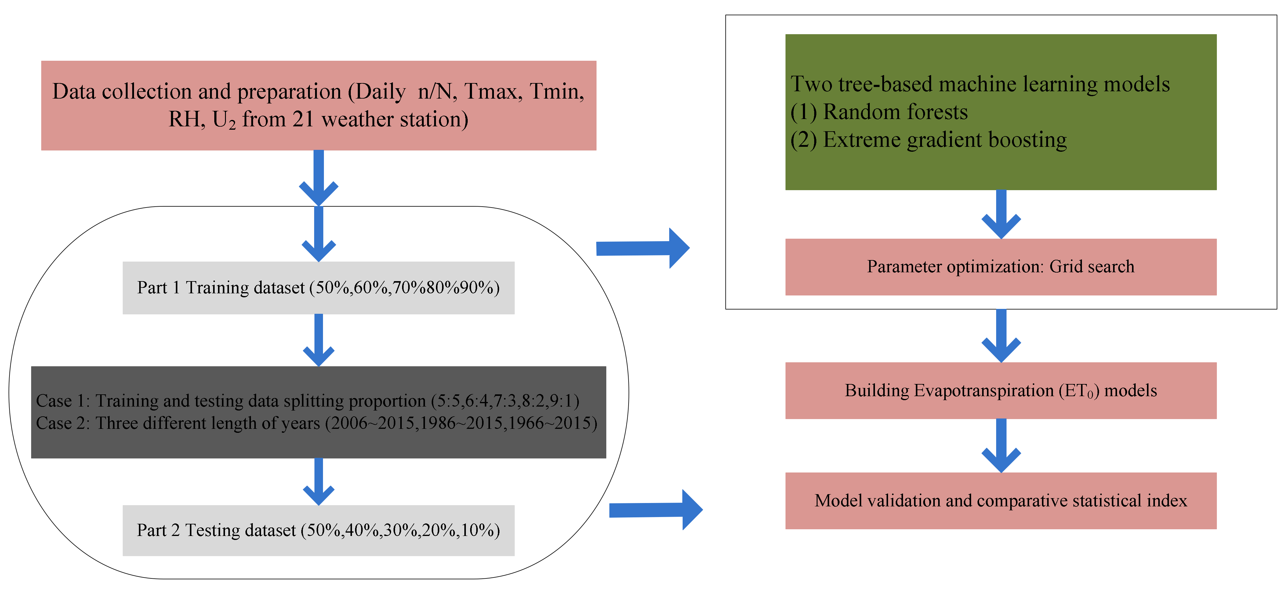
2. Materials and Methods
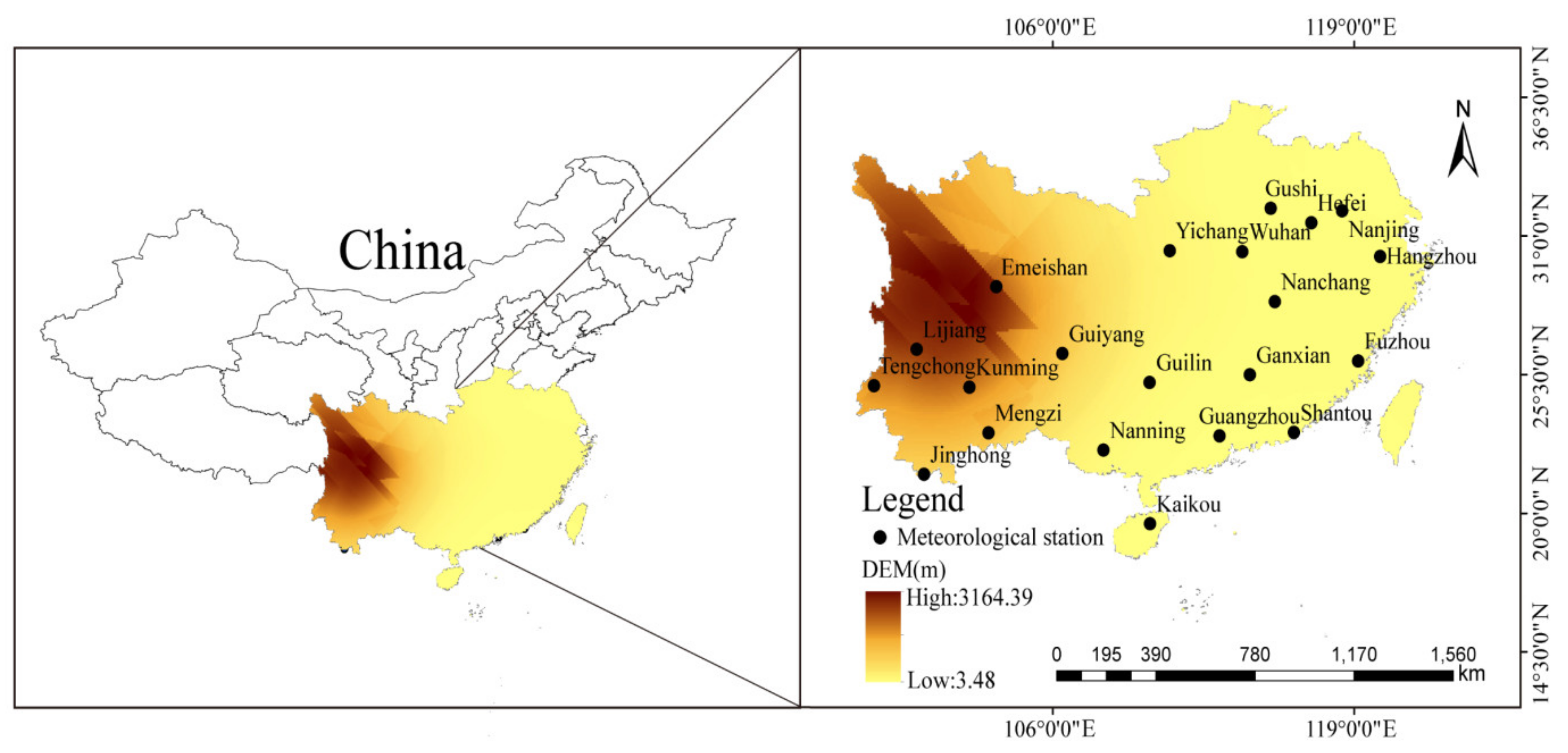
2.1. Study Areas

In this research, daily meteorological data from 21 representative meteorological stations across the humid region of China (Figure 1) were used to build the RF and XGB models to estimate ET0. This area is rich in water and heat resources, the geographic range including two river basins (the Yangtze River Basin and the Pearl River Basin). Due to the effect of El Nino and typhoons, the occurring frequency of floods and waterlogging disasters in this region is generally high, often bringing huge impacts to nature and the society of this region. For example, a summer flood that occurred in the Poyang Lake of the Yangtze River Basin affected over 2.531 million people and 190.4 thousand hectares of crops, resulting in an economic loss of 2.39 billion RMB. Therefore, this area has become an area of widespread concern for many scholars who study hydrological phenomena and climate [55,91].

2.2. Used Temperature Data

Continuous and long-term series of observed daily maximum (Tmax) and minimum (Tmin), relative humidity (RH), global solar radiation (Rs), extra-terrestrial solar radiation (Ra), and wind speed (U2) from 1966 to 2019 were gathered from 21 representative climatological stations in the humid region of China (Figure 1). Among them, 1966–2015 was used for training and testing models, and 2016–2019 was used for independent testing. The meteorological records with quality control were obtained from the National Meteorological Information Center (NMIC) of China Meteorological Administration (URL: http://data.cma.cn accessed on 5 March 2020). The detailed description of the 21 studied weather stations is listed in Table 1. Among these stations, the mean daily maximum ambient temperatures were 7.75–29.75 °C, and the mean daily minimum ambient temperatures were 0.55–21.65 °C. The range of daily average wind speed varied from 0.49 to 2.37 m·s−1, while the daily average relative humidity ranged between 85.51% at Emeishan and 62.43% at Lijiang. The range of daily average global solar radiation varied between 16.94 MJ·m−2·d−1 at Lijiang and 10.15 MJ·m−2·d−1 at Guiyang. The highest daily average ET0 (3.44 mm·d−1) was monitored at Mengzi, while the lowest value (1.72 mm·d−1) appeared at Emeishan. In general, the plateau site is more variable than sites in plains and hilly areas.

2.3. Estimation of Reference Evapotranspiration Using the FAO-56 Penman–Monteith Equation

The Penman–Monteith equation advocated by Allen et al. was used to compute daily ET0 [3] and provide the reference evapotranspiration for the machine learning models in this study [62,88,92]:
E T 0 = 0.408 Δ R n G + γ 900 T m e a n + 273 U 2 e s e a Δ + γ 1 + 0.34 U 2
where Rn: net radiation (MJ·m−2·d−1); G: soil heat flux (MJ·m−2·d−1); Tmean: average ambient temperature (°C), i.e., Tmean = (Tmax + Tmin)/2; U2: wind speed (m·s−1); es: saturation vapor pressure (kPa); ea: actual vaporpressure (kPa); Δ: slope of the vapor pressure curve (kPa °C−1), and γ: psychrometric constant (kPa °C−1). For more details on how Penman–Monteith equation was constructed, please refer to the literature of Allen et al. [3].

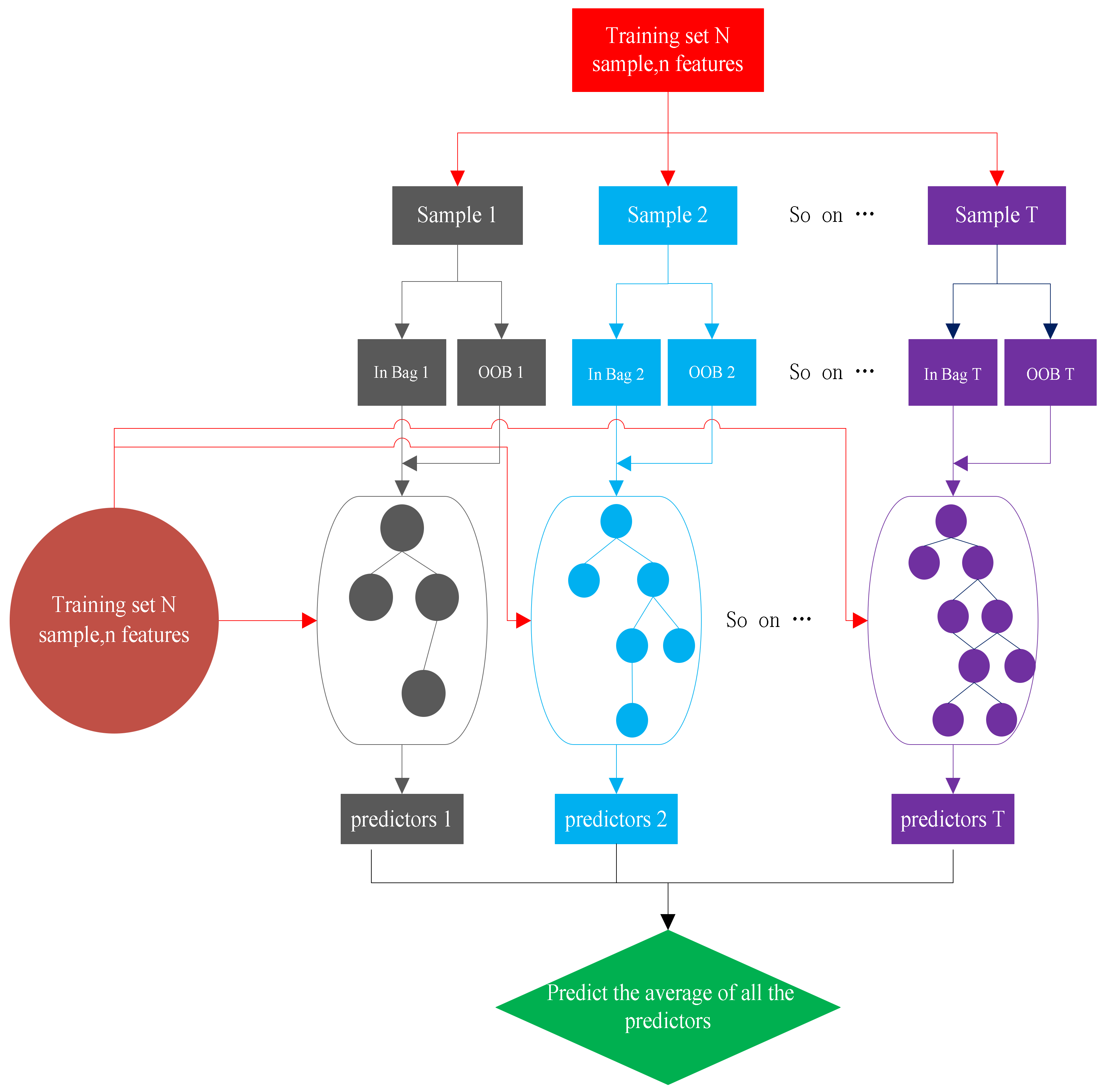
2.4. Random Forest (RF)

Random forest (RF) is used for classification and regression [7], mainly used for regression problems [55,91,93]. The RF algorithm builds a decision tree on data samples and then obtains the prediction results from each sample, reduces overfitting by averaging the results, and finally optimizes the solution, thereby improving the prediction performance.
The model of random forest is established by decision-based learning device. To establish an RF model, the first step is to get the sub-training set from the original data. Suppose there are M samples in the initial dataset D, and the probability of not selecting a particular individual after M samples is (1-M1)M. This means that when the training sets are generated by sampling, each training set contains 63.2% of the original datasets, and the unselected ones (36.8% of the original datasets) become out-of-bag datasets.
The main difference between random forest and bagging is that, when constructing each tree, n features are randomly selected from all the features M. When optimizing each segmentation node, the principle of minimum Gini coefficient is adopted. The Gini coefficient can be expressed as follows:
G i n i p = 2 p 1 p
For the classification problem, the original problem began with developing trees on the basis of random vector when using RF [7]. The prediction ability of the random forest model needs to be evaluated by the edge function, and the equation is as follows:
m g X , Y = a v k I h k X = Y m a x j Y a v k I h k X = j
Generalization error is used to measure the accuracy of the random forest model. The generalization error of random forest is:
P E * = P X , Y m g X , Y < 0
For the parameter meaning in the above formula and the details of the random forest model establishment, please refer to the literature of Breiman [7]. The structure of the RF algorithm is shown in Figure 2.

2.5. Extreme Gradient Boosting

Extreme gradient boosting (XGB) is a new algorithm of gradient enhancers (GBMs) proposed by Chen and Guestrin [9]. The XGB model is designed to prevent over-fitting while reducing the computational cost by keeping the predictions at the best computational efficiency through simplification and regularization. The XGB algorithm is derived from the concept of “boosting”. It combines all the predictions of a group of weak learners and trains strong learners through special training. The calculation formula is as follows:
f i t = k = 1 t f k x i = f i t 1 + f t x i
where t is the number of trees, ft(xi) is a function, and xi is the input variable.
In order to prevent the over-fitting problem without affecting the calculation speed of the model, the XGB model can derive the following formula:
O b j t = k = 1 n l y i ¯ , y i + k = 1 n Ω f i
where l is loss function, n is the number of the observed, k = 1 n l y i ¯ , y i is training error, y i ¯ is the predicted value, yi is the actual value, Ω is the regularization term, and the formula is:
Ω f = γ T + 1 2 λ ω 2
where ω is norm of leaf scores, λ is a regularization parameter, and γ represents the parameter that controls the weight of the number of leaves.
The XGB algorithm is based on a gradient boosting strategy. It does not reach all the trees at once but adds a new tree each time to patch the previous test results. Assuming that the predicted value at step t is y i ( t ) , the following derivation process can be obtained:
y i ( 0 ) = 0 y i ( 1 ) = f 1 ( x i ) = y i ( 0 ) + f 1 ( x i ) y i ( 2 ) = f 1 ( x i ) + f 2 ( x i ) = y i ( 1 ) + f 2 ( x i ) y i ( t ) = k = 1 t f k ( x i ) = y i ( t 1 ) + f t ( x i )
Details of the XGB model can be found in Song et al. [94].

2.6. Input Combinations

Four input combinations of meteorological variables were applied in present research to discuss the influences of different climatic factors on daily ET0 estimation. Therefore, utilizing various combinations of Tmax, Tmin, Ra, Rs, RH, and U2, a total of four combinations of input are considered (Table 2). The flowchart of this study is described in Figure 3.

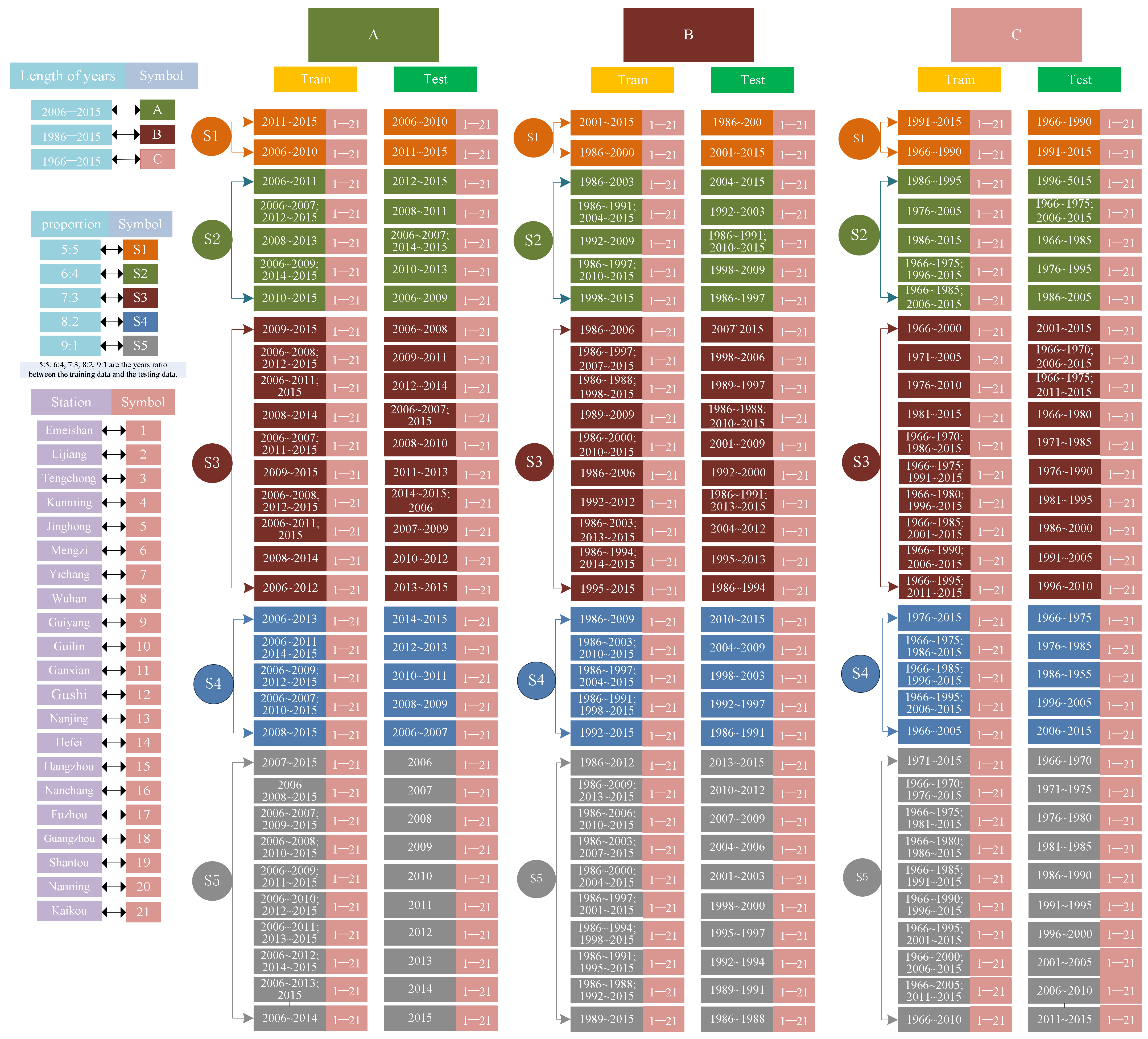
2.7. Data Splitting Strategies and Time Lengths of Input Data

In this study, five data splitting strategies with different proportions of datasets allocated for model training and testing were applied. Specifically, the proportions of dataset allocating to training and testing stages were set as 5:5 (S1), 6:4 (S2), 7:3 (S3), 8:2 (S4), and 9:1 (S5), respectively (Figure 4). Within each of the splitting strategies, three levels of data with different time ranges (spanning 10, 30, and 50 years, respectively) were used for model development and evaluation, which were defined as the 10-year span (2006–2015), the 30-year span (1986–2015), and the 50-year span (1966–2015), respectively (Figure 4). Details of the data splitting strategy, the selection of specific years, and the cross-validation procedure for the establishment and evaluation of each model are shown in Figure 4. Furthermore, this paper used a fixed test dataset from 2016 to 2019 for independent testing and varying only the training dataset. Based on the above data manipulation, the machine learning models coupled with a K-fold cross-validation approach was then applied to estimate ET0 under each of the input combinations.

2.8. Statistical Performance Analysis

The accuracy of the models for estimating daily ET0 were evaluated with four generally used statistical indicators [64,91], which were root mean square error (RMSE), mean absolute error (MAE) [95], coefficient of determination (R2), and Nash–Sutcliffe coefficient (NSE) [96], respectively. The statistical indices are expressed as follows:
R M S E = 1 n i = 1 n ( X i , P X i . , R ) 2
M A E = 1 n i = 1 n X i , P X i , R
R 2 = i = 1 n X i , P X ¯ i , P X i , R X ¯ i , R 2 i = 1 n X i , P X ¯ i , P 2 i = 1 n X i , R X ¯ i , R 2
N S E = 1 i = 1 n X i , p X i , R 2 i = 1 n X i , p X i , R 2
where Xi,P, Xi,R, X ¯ i , P , and n are the FAO-56 Penman–Monteith ET0, the predicted ET0, the mean of FAO-56 Penman–Monteith ET0, and the number of observed meteorological data, respectively. The value of R2 exceedingly approaches 1, meaning the model has better performance and data fitting. Conversely, the values of RMSE and MAE extremely approach 0, indicating higher prediction accuracy. Sutcliffe coefficient (NSE) is a commonly used indicator when evaluating the performance of a model. The higher the value of NSE, the better the performance of the model and vice versa. A perfect well between the estimated and the target ET0 will produce NSE = 1.0 [97].

3. Results

3.1. Comparisons of XGB and RF Predicting Daily ET0 with Various Input Combinations

The predicting capability of machine learning models for reference evapotranspiration at three levels of time length (2006–2015, 1986–2015, and 1966–2015) was evaluated by the R2, RMSE, MAE, and NSE, which is largely due to the input of meteorological data, These meteorological data are derived from the FAO-56 Penman–Monteith model. The statistical results of the four different input combinations for predicting the daily ET0 at the twenty-one climatological stations in the humid areas of China are provided in Table 3.
Taking the 50-year span as an example, the RF and XGB models with input combination 2 (i.e., the RF2 and XGB2 models, input variables consisting of Tmax, Tmin, and Rs) had better predicting accuracy than the other input combinations (Table 3); the range of the mean RMSE value of the two combinations (inputs with Tmax, Tmin, and Rs; inputs with Tmax, Tmin, and Ra, respectively) were 0.324–0.688 mm d−1 during the testing phase, and the homologous values of the XGB models were 0.328–0.689 mm d−1. The input combination of Tmax, Tmin, RH, and Ra produced a pleasing daily ET0 prediction, and the mean RMSE values were 0.516 mm d−1 and 0.526 mm d−1 in the RF and XGB, respectively. Whereas, the models with input combination 4 (i.e., input variables consisting of Tmax, Tmin, U2, and Ra) were also capable of estimating the daily ET0 with respectable precision, possessing a mean RMSE value of 0.607 mm d−1 and 0.620 mm d−1 in the RF and XGB, respectively. These phenomena show that a reasonable combination of parameters is beneficial to the improvement of model accuracy. On the basis of temperature variables, the importance for each of the other three meteorological variables (i.e., Rs, RH, and U2) contributing to the improvement of model accuracy can be ranked as Rs > RH > U2. Although the input combination with Rs can produce better model accuracy than input combinations with any other variable, it should be noted that the radiation records are not universally available across the world, especially for less developed regions. In comparison, RH is a variable that could be easily obtained in most regions on Earth, while, at the same time, it provides a decent contribution to improving model accuracy. Therefore, RH is recommended as an alternative for ET0 estimation with the model in regions where Rs is not available. In terms of machine learning models’ performance under different input combinations, compared with the 50-year span, similar patterns were observed in the other two levels of time range, and the random forest model is better than the extreme gradient boosting model (i.e., the 10-year span and the 30-year span, respectively; see Table 3).

3.2. Comparisons of XGB and RF Predicting Daily ET0 with Data Splitting Proportions

Table 4, Table 5 and Table 6 present the statistical results of the machine learning models with the five data splitting strategies (i.e., splitting into proportions of 5:5 (S1), 6:4 (S2), 7:3 (S3), 8:2 (S4), and 9:1 (S5), respectively) under four combinations of input during testing phases. As shown in the tables, the models predicting accuracy differ among data splitting strategies under the same input combination. Using the 50-year span (Table 6) as an example, the S5 proportion demonstrated that the values of R2 and NSE are closest to 1 and the values of RMSE and MAE are closest to 0 in the testing phase for the four combinations of input in two machine learning models, compared to the S4, S3, S2, and S1. The ranks of the researching proportions of the two machine learning models in the field of estimation precision in the testing phase were: S5 > S4 > S3 > S2 > S1. In other words, the S5 proportion had a slightly better capability than the S4 proportion and S3 proportion while realizing a greater edge in capability over the S2 proportion and the S1 proportion. The S5 and S4 proportions had almost equivalent performance (distinction in RMSE < 2%) in predicting the daily ET0 for the four combinations of input, both of which move beyond the other three data splitting proportions in estimating the daily ET0. However, the S1 proportion of XGB and RF revealed the worst estimates of the daily ET0 for the S5 proportion, with an increase in RMSE by 7.5–7.6% and 7.1–7.2% for the combination of input (i.e., Tmax, Tmin, Ra, and RH) and only by 3.5–5.9% and 2.6–5.0% for the other three input combinations, respectively. In general, for the five data splitting proportions, the statistical performance of the data splitting proportion of the RF is better than that of the XGB (Table 6), indicating that the random forest models produced high-precision estimation at the testing. Compared with the 50-year span, similar patterns of model performance with different data splitting proportions were observed in the 10-year span (Table 4) and the 30-year span (Table 5).
The box diagrams of the FAO-56 Penman–Monteith ET0 values and ET0 predicted by the RF model of the model of the S5 proportion during ten cross-validation periods using the best combination of input (i.e., the combination of Tmax, Tmin, and Rs) in the testing phase are demonstrated in Figure 5. The diagrams clearly presented that the scopes of ET0 values estimated by the ten cross-validation stages were close to the FAO-56 Penman–Monteith ET0 values of their corresponding stages, further highlighting the model accuracy on estimating daily ET0. Overall, the accuracy of the ten cross-validation periods for the four selected sites was high, suggesting that the RF model can be utilized for estimating ET0 in this area. In particular, the medians, inter-quartile ranges, and extreme values of the fifth and six cross-validation periods were closer to their corresponding values of FAO-56 Penman–Monteith than other cross-validation periods, indicating a better daily ET0predicting performance for the former two periods. Among the four selected sites, the distribution of the maximum, minimum, and interquartile range values of the ET0 at Guiyang station (inland plateau) was the closest to the corresponding values of the FAO-56 PM estimated ET0 during the ten cross-validation stages.

3.3. Comparisons of XGB and RF Predicting Daily ET0 with Various Time Lengths of Input Data

The average and local RMSE values of the RF and XGB models for estimating daily ET0 using the available length of years variables in the testing stage at the meteorological stations in the humid regions of southern China are presented in Figure 6. Similar to previous results (Table 3), the machine learning models with input combination 2 (i.e., the RF2 and XGB2 models, input variables consisting of Tmax, Tmin, and Rs) and the data spitting proportion of S5 had more promising accuracy than other models and proportions. Specifically, under the different data splitting strategies in the testing stage, compared to the 10-year dataset, the increased percentage of the average RMSE of the RF2 model datasets from a length of 50 years ranged from 2.811 to 3.21%, while the increased percentage of the average RMSE of the 30-year dataset increased by 0.39 to 0.74% in the RF2 model. Besides, the ranges of the increased percentage in the RF1, RF3, and RF4 models were 3.16–3.56%, 6.21–7.07%, and 1.01–1.24%; 0.58–0.79%, 0.45–1.89%, and 0.46–0.84% in the field of the average RMSE in the length of 50 years and length of 30 years datasets relative to the 10-year dataset, respectively. Moreover, the extreme gradient boosting model is consistent with the results shown by the random forest model. Compared to the 30-year dataset, the increased percentage of the average RMSE in the XGB2 model datasets from a length of 50 years ranged from 3.45–3.78%, while the decreased percentage of average RMSE of a 10-year dataset decreased by 2.85–3.30%. Among the three levels of time lengths of input data, the XGB and RF models with the 50-year span performed worst (RMSE = 0.276 mm·d−1–0.612 mm·d−1 and 0.259 mm·d−1–0.572 mm·d−1, respectively), followed by the 30-year span (with RMSE ranging 0.266 mm·d−1–0.593 mm·d−1 and 0.252 mm·d−1–0.557 mm·d−1, respectively); the 10-year span (2006–2015) showed satisfying daily ET0 estimates in southern China (RMSE = 0.257 mm·d−1–0.579 mm·d−1 and 0.250 mm·d−1–0.554 mm·d−1, respectively). Overall, under the same ratios and combinations of the RMSE values of the three time spans, the reduction in the modeling data used improves the accuracy of the XGB and RF models (Figure 6).

3.4. Comparisons of XGB and RF Predicting Daily ET0 with a Fixed Testing Dataset

To effectively assess the impacts of different data splitting proportions and various time lengths of input data on model performance, a fixed testing dataset consisting of records from 2016 to 2019 was used for the model testing of all the types of models constructed in this study. Meanwhile, the training datasets remained varied among different models, the same as stated previously. The average statistical indicators of models with the fixed testing dataset (2016–2019) were calculated for different time lengths of input data (Table 7, Table 8 and Table 9). As shown in the tables, under the same time length of input data, both the RF and XGB models with input combination 2 (i.e., the RF2and XGB2 models, input variables consisting of Tmax, Tmin, and Rs) had better predicting accuracy than other input combinations, and this pattern did not vary among different time lengths. Furthermore, for any of the three time lengths, the estimating accuracies of the two groups of machine learning models with different data splitting proportions was ranked as S5 > S4 > S3 > S2 > S1. Specifically, compared with other splitting proportions, the values of R2 and NSE were closer to 1, while the values of RMSE and MAE were closer to 0 in the S5 proportion during the testing phase for any of the four input combinations, and these trends did not differ between the RF and XGB models. The results with the fixed testing dataset were consistent with the results of the above testing datasets (Table 4, Table 5 and Table 6).
To evaluate the impacts of different time lengths of input data on model accuracy, the statistical indicators of models with the fixed testing dataset (2016–2019) under the input combination 2 and the S5 proportion were analyzed (Figure 7). Generally, RF showed higher accuracy than XGB. Under each of the three time lengths, the RF model consistently had higher values of R2 and NSE and lower RMSE and MAE values than the XGB model (Figure 7). Among the three time lengths, the models with the 30-year span data showed the best estimating accuracy, followed by models with the 50-year span data and then with the 10-year span data, respectively. Taking the RF model as an example, the values of R2 (0.951) and NSE (0.946) for the models with the 30-year span data were higher than models with the 50-year span data (R2 = 0.950; NSE = 0.944), or the same as models with the 10-year span data (R2 = 0.951; NSE = 0.946). Meanwhile, the 10-year-span models had lower error values (RMSE = 0.312 mm·d−1; MAE = 0.234 mm·d−1) than models with other time spans (RMSE = 0.313 mm·d−1 and MAE = 0.237 mm·d−1 for the 50-year span; RMSE = 0.317 mm·d−1 and MAE = 0.238 mm·d−1 for the 10-year span). The results for other input combinations and other data splitting proportions (see Tables S1 and S2 for details) were consistent with the above results.

4. Discussion

4.1. Effects of Input Combination Strategy on Daily ET0 Estimation

The category of the parameters of input was a crucial factor for the estimation precision of the machine learning models in estimating the daily ET0. The model commonly operated the worst when the Tmax/Tmin and Ra were valid in southern China. Since the model prediction accuracy generally increases with the more meteorological input parameters [57,98,99], models with temperature data as inputs would only generate non-ideal daily ET0 estimation despite the fact that temperature data are generally widely effective around the world [20,100]. Therefore, the extreme gradient boosting and random forest model with wind speed, relative humidity, and global solar radiation (instead of extra-terrestrial radiation) data would produce acceptable ET0 values. In this study, the machine learning models with the input combination of Tmax, Tmin, and Rs presented better prediction accuracy than other combinations. The results indicate that, with the global solar radiation (Rs) as inputs, the ET0 values estimated by the XGB and RF models show a favorable viewpoint with the homologous FAO-56 Penman–Monteith values in the humid regions of China. Feng et al., Fan et al. and Huang et al. also demonstrated that the random forest models with Tmax/Tmin and Rs attained extremely pleasing ET0 estimation in southern China [54,55,62]. The XGB and RF models with Tmax/Tmin, Ra, and RH outperformed the XGB and RF models with Tmax/Tmin, Ra, and U2 in the humid region. These consequences indicate that relative humidity is a more important factor than wind speed when estimating the ET0 with the XGB and RF models in the humid region. Among the three single factors other than temperature, the significance of meteorological parameters to estimate daily ET0 was ranked as Rs > RH > U2 in the humid area of southern China. This consequence is consistent with the research of Yan et al. [78], where they conclude that Rs is more influential than RH and U2 for estimating the daily ET0 in the humid region.

4.2. Effects of Data Splitting Proportions on Daily ET0 Estimation

Previous studies have shown that high-precision simulations of machine learning models on ET0 prediction can be obtained with a single ratio of allocating data into training and testing [56,61]. However, under the same total dataset, there is no report on whether the multiple ratios between the training data and testing data will improve the precision of the machine learning models. As mentioned above (see in Table 4, Table 5 and Table 6, respectively), the extreme gradient boosting and random forest models with the data splitting proportion of S5 showed excellent capability in predicting the daily ET0 for all the combinations of input, which exceeded the other four data splitting proportions at twenty-one meteorological stations during the testing phase. Moreover, as the number of years in the testing phase decreases, the accuracy of the model increases. This is an exceedingly hopeful strategy for improving the accuracy of machine learning models to estimate daily ET0, especially when there are plenty of historical years of data in the training phase. Consequently, for improving the accuracy of machine learning models, the models should be established with appropriate data segments. In this research, the five proportions among the proportions within the dataset were identified. The accuracy of the data-segment increased with the increase in the ratio in five ratios. In the split rule cases of Rezaabad et al. [101], the three nearest proportions among the proportions within the ten percent of the dataset were also identified. The accuracy of the smallest data segment has been known as the inferior ratio in the three ratios. However, the accuracy of the maximum proportion of this study is not perfect. Therefore, how to precisely select a satisfying proportion needs further study. Shiri et al. established the GEP model, utilizing data splitting strategies in sub-humid stations for estimating the daily ET0, and procured good results in sub-humid regions [102]. However, in this study, the XGB and RF models were evaluated in humid areas. Future studies will be needed to use coupled data from arid and humid stations for evaluating the machine learning models.

4.3. Effects of Available Length of Years on Daily ET0 Estimation

The average RMSE calculated by the period of the length of the 10-year dataset was much lower than those of the corresponding two periods under various combinations and proportions, while the length of the 50-year dataset was the highest (Figure 6). The results indicated that the reduced use of modeling data can improve the accuracy of the precision of the random forest models under various input parameters and data segmentation. This shows that the length of 50 years has been particularly inaccurate in dealing with the complex non-linear relationship between the ET0 and its parameters in the XGB and RF models, The reason for this phenomenon may be that climate change has caused changes in meteorological factors, resulting in a corresponding increase in the value of the ET0 with the growing length of years. Related phenomena have also been reported in the literature [85,86,103]. However, the results of independent testing data show that the model with a 30-year span has the highest accuracy and the model with a 10-year span has the lowest (Figure 7), which is inconsistent with the results shown in the test dataset. The reason for this phenomenon may be due to the over-fitting phenomenon caused by the smaller dataset of the 10-year span model [104]. In this study, the results showed that appropriately reducing the year span of the dataset is beneficial for the improvement of the model accuracy. However, the specific causes remain to be further studied. In addition, the superiority of datasets of different lengths for predicting ET0 has been widely researched [105]. Yin et al. coupled the bi-directional and different datasets for predicting the ET0 and discovered that the length of the short dataset provides the best forecast performance in three lengths of datasets [106]. In the present study, the three different lengths of years were used to build extreme gradient boosting and random forest models for the first time. Due to the variables of different lengths of years, the prediction precision of the random forest and extreme gradient boosting models have been enhanced (Figure 6 and Figure 7). Although the 10-year meteorological data obtained high accuracy in the test dataset, its performance was the worst in independent testing. Therefore, the 30-year data span model is a promising method for predicting the ET0 in the humid southern regions of my country, and it may also apply to regions with similar climates.

5. Conclusions

The extreme gradient boosting and random forest models of data splitting strategies and variable ranges of years have been put forward to predict the daily ET0 in twenty-one weather stations of the humid regions of China. The results revealed that the accuracy of the random forest model is better than that of the extreme gradient boosting model, and the Rs were more crucial than the RH, U2, and Ra in predicting the daily ET0 in southern China. The data splitting proportion of S5 showed excellent performance for all the same input combinations, and the importance of the data splitting variables for predicting the daily ET0 was as follows: S5 > S4 > S3 > S2 > S1. Compared with the length of 30 years, the estimation accuracy of the 50-year length with limited data is reduced, while the length of meteorological data of 10 years improves the accuracy for southern China. However, the 10-year performance was worse when considering the independent test. Considering that the data span of 30 years has high accuracy and a stable performance, it is recommended that the random forest model with a dataset of 30-year length produces the daily ET0. In the absence of continuous and complete meteorological records, this promising strategy can be used as an alternative to the FA0-56 P-M model to calculate ET0. Consequently, the random forest model is proposed as a hopeful selective approach to improving the accuracy for estimating the daily ET0 under conditions of insufficient climatic data in the humid area of southern China. Whereas, further research is required to estimate the performance of the suggested random forest model in the arid and humid climate areas of China or similar climates around the world.

Supplementary Materials

The following are available online at https://www.mdpi.com/article/10.3390/w13233478/s1, Table S1. Average statistical values of different input parameters of three length of years of machine learning models in testing process of 21 stations under the fixed test data set (2016-2019). Table S2. Average statistical values of five proportions of three length of years of machine learning models in testing process of 21 stations under the fixed test data set (2016-2019).

Author Contributions

X.L.: Data curation, Formal analysis, Software, Validation, Funding acquisition, Writing—original draft, Writing—review & editing. F.Z.: Formal analysis, Writing-review & editing. L.W.: Conceptualization, Methodology, Software, Writing-review & editing. G.H.: Writing—review & editing. F.Y.: Data curation, Formal analysis. W.B.: Data curation, Formal analysis. All authors have read and agreed to the published version of the manuscript.

Funding

This research was funded by “National Key Research and Development Program of China, grant number 2017YFC1502701” and “Science and technology Cooperation Project in Jiangxi of China, grant number 20212BDH80016”.

Institutional Review Board Statement

Not applicable.

Informed Consent Statement

Not applicable.

Data Availability Statement

All data will be made available on request to the correspondent author’s email with appropriate justification.

Acknowledgments

Thanks to the National Meteorological Information Center of China Meteorological Administration for offering the meteorological data.

Conflicts of Interest

The authors declare that they have no conflict of interest to influence the work reported in this paper.

References

  1. Abdullah, S.S.A.; Malek, M.A.; Abdullah, N.S.; Kisi, O.; Yap, K.S. Extreme learning machines: A new approach for prediction of reference evapotranspiration. J. Hydrol. 2015, 527, 184–195. [Google Scholar] [CrossRef]
  2. Fan, J.; Oestergaard, K.T.; Guyot, A.; Lockington, D.A. Estimating groundwater recharge and evapotranspiration from water table fluctuations under three vegetation covers in a coastal sandy aquifer of subtropical Australia. J. Hydrol. 2014, 519, 1120–1129. [Google Scholar] [CrossRef] [Green Version]
  3. Feng, Y.; Peng, Y.; Cui, N.; Gong, D.; Zhang, K. Modeling reference evapotranspiration using extreme learning machine and generalized regression neural network only with temperature data. Comput. Electron. Agric. 2017, 136, 71–78. [Google Scholar] [CrossRef]
  4. Traore, S.; Luo, Y.; Fipps, G. Deployment of artificial neural network for short-term forecasting of evapotranspiration using public weather forecast restricted messages. Agric. Water Manag. 2016, 163, 363–379. [Google Scholar] [CrossRef]
  5. Karimi, S.; Shiri, J.; Mart, P. Supplanting missing climatic inputs in classical and random forest models for estimating reference evapotranspiration in humid coastal areas of Iran. Comput. Electron. Agric. 2020, 176, 105633. [Google Scholar] [CrossRef]
  6. Priestley, C.H.B.; Taylor, R.J. On the assessment of surface heat flux and evaporation using large-scale parameters. Mon. Weather Rev. 1972, 100, 81–92. [Google Scholar] [CrossRef]
  7. Djaman, K.; Tabari, H.; Balde, A.B.; Diop, L.; Futakuchi, K.; Irmak, K. Analyses, calibration and validation of evapotranspiration models to predict grass-reference evapotranspiration in the Senegal river delta. J. Hydrol. Reg. Stud. 2016, 8, 82–94. [Google Scholar] [CrossRef] [Green Version]
  8. Feng, Y.; Cui, N.; Zhao, L.; Hu, X.; Gong, D. Comparison of ELM, GANN, WNN and empirical models for estimating reference evapotranspiration in humid region of Southwest China. J. Hydrol. 2016, 536, 376–383. [Google Scholar] [CrossRef]
  9. Karimi, S.; Kisi, O.; Kim, S.; Kim, S.; Nazemi, A.; Shiri, J. Modelling daily reference evapotranspiration in humid locations of South Korea using local and cross-station data management scenarios. Int. J. Climatol. 2017, 37, 3238–3246. [Google Scholar] [CrossRef]
  10. Yan, S.; Wu, Y.; Fan, J.; Zhang, F.; Qiang, S.; Zheng, J.; Xiang, Y.; Guo, J.; Zou, H. Effects of water and fertilizer management on grain filling characteristics, grain weight and productivity of drip-fertigated winter wheat. Agric. Water Manage. 2019, 213, 983–995. [Google Scholar] [CrossRef]
  11. Guitjens, J.C. Models of Alfalfa yield and evapotranspiration. J. Irrig. Drain. Div. Proc. Am. Soc. Civ. Eng. 1982, 108, 212–222. [Google Scholar] [CrossRef]
  12. Harbeck, G.E., Jr. A Practical Field Technique for Measuring Reservoir Evaporation Utilizing Mass-Transfer Theory; Paper 272-E; US Government Printing Office: Washington, DC, USA, 1962; pp. 101–105.
  13. Allen, R.G.; Pereira, L.S.; Raes, D.; Smith, M. Crop Evapotranspirationguidelines for Computing Crop Water requirements-FAO Irrigation and Drainage Paper 56. Fao Rome 1998, 300, D05109. [Google Scholar]
  14. Doorenbos, J.; Pruitt, W.O. Guidelines for predicting crop water requirements. In FAO Irrigation and Drainage Paper 24; FAO: Rome, Italy, 1977. [Google Scholar]
  15. Monteith, J.L. Evaporation and environment. In Symposia of the Society for Experimental Biology; Society for Experimental Biology: London, UK, 1965; Volume 19, pp. 205–234. [Google Scholar]
  16. Penman, H.L. Natural evaporation from open water, hare soil and grass. Proc. R. Soc. Lond. 1948, 193, 120–145. [Google Scholar]
  17. Fan, J.; Wang, X.; Wu, L. New combined models for estimating daily global solar radiation based on sunshine duration in humid regions: A case study in South China. Energy Convers. Manage. 2018, 156, 618–625. [Google Scholar] [CrossRef]
  18. Fan, J.; Chen, B.; Wu, L. Evaluation and development of temperature-based empirical models for estimating daily global solar radiation in humid regions. Energy 2018, 144, 903–914. [Google Scholar] [CrossRef]
  19. Shiri, J.; Nazemi, A.H.; Sadraddini, A.A.; Landeras, G.; Kisi, O.; Fard, A.F.; Marti, P. Comparison of heuristic and empirical approaches for estimating reference evapotranspiration from limited inputs in Iran. Comput. Electron. Agric. 2014, 108, 230–241. [Google Scholar] [CrossRef]
  20. Feng, Y.; Jia, Y.; Cui, N.; Zhao, L.; Li, C.; Gong, D. Calibration of Hargreaves model for reference evapotranspiration estimation in Sichuan basin of south-west China. Agric. Water Manage. 2017, 181, 1–9. [Google Scholar] [CrossRef]
  21. Jensen, D.T.; Hargreaves, G.H.; Temesgen, B.; Allen, R.G. Computation of ET0 under non ideal conditions. J. Irrig. Drain. Eng. 1997, 123, 394–400. [Google Scholar] [CrossRef]
  22. Martí, P.; Zarzo, M.; Vanderlinden, K.; Girona, J. Parametric expressions for the adjusted Hargreaves coefficient in Eastern Spain. J. Hydrol. 2015, 529, 1713–1724. [Google Scholar] [CrossRef]
  23. Mendicino, G.; Senatore, A. Regionalization of the Hargreaves coefficient for the assessment of distributed reference evapotranspiration in Southern Italy. J. Irrig. Drain Eng. 2013, 139, 349–362. [Google Scholar] [CrossRef]
  24. Barzkar, A.; Najafzadeh, M.; Homaei, F. Evaluation of drought events in various climatic conditions using data-driven models and a reliability-based probabilistic model. Nat. Hazards 2021, 1–22. [Google Scholar] [CrossRef]
  25. Dong, J.; Wu, L.; Liu, X.; Li, Z.; Gao, Y.; Zhang, Y.; Yang, Q. Estimation of daily dew point temperature by using bat algorithm optimization based extreme learning machine. Appl. Therm. Eng. 2020, 165, 114569. [Google Scholar] [CrossRef]
  26. Fan, J.; Wang, X.; Wu, L. Comparison of support vector machine and extreme gradient boostinging for predicting daily global solar radiation using temperature and precipitation in humid subtropical climates: A case study in China. Energy Convers. Manage. 2018, 164, 102–111. [Google Scholar] [CrossRef]
  27. Fan, J.; Wu, L.; Zhang, F. Evaluating the effect of air pollution on global and diffuse solar radiation prediction using support vector machine modeling based on sunshine duration and air temperature. Renew. Sustain. Energy Rev. 2018, 94, 732–747. [Google Scholar] [CrossRef]
  28. Kaba, K.; Sarıgül, M.; Avcı, M.; Kandırmaz, H.M. Estimation of daily global solar radiation using deep learning model. Energy 2018, 162, 126–135. [Google Scholar] [CrossRef]
  29. Keshtegar, B.; Mert, C.; Kisi, O. Comparison of four heuristic regression techniques in solar radiation modeling: Kriging method vs RSM, MARS and M5 model tree. Renew. Sustain. Energy Rev. 2018, 81, 330–341. [Google Scholar] [CrossRef]
  30. Kim, S.; Singh, V.; Lee, C.; Seo, Y. Modeling the physical dynamics of daily dew point temperature using soft computing techniques. KSCE J. Civ. Eng. 2015, 19, 1930–1940. [Google Scholar] [CrossRef]
  31. Mehdizadeh, S.; Behmanesh, J.; Khalili, K. Application of gene expression programming to predict daily dew point temperature, Appl. Therm. Eng. 2017, 112, 1097–1107. [Google Scholar] [CrossRef]
  32. Movahed, S.F.; Najafzadeh, M.; Mehrpooya, A. Receiving More Accurate Predictions for Longitudinal Dispersion Coefficients in Water Pipelines: Training Group Method of Data Handling Using Extreme Learning Machine Conceptions. Water Resour. Manag. 2020, 34, 529–561. [Google Scholar] [CrossRef]
  33. Najafzadeh, M.; Niazmardi, S. A Novel Multiple-Kernel Support Vector Regression Algorithm for Estimation of Water Quality Parameters. Nat. Resour. Res. 2021, 5, 3761–3775. [Google Scholar] [CrossRef]
  34. Singh, K.P.; Basant, N.; Gupta, S. Support vector machines in water quality management. Anal. Chim. Acta 2011, 703, 152–162. [Google Scholar] [CrossRef] [PubMed]
  35. Sun, D.; Li, Y.; Wang, Q. A unified model for remotely estimating chlorophyll a in Lake Taihu, China, based on SVM and in situ hyperspectral data. IEEE Trans. Geosci. Rem. Sens. 2009, 47, 2957–2965. [Google Scholar]
  36. Wang, L.; Niu, Z.; Kisi, O.; Kisi, O.; Li, C.; Yu, D. Pan evaporation modeling using four different heuristic approaches. Comput. Electron. Agric. 2017, 140, 203–213. [Google Scholar] [CrossRef]
  37. Wang, L.; Kisi, O.; Hu, B.; Bilal, M.; Kermani, M.; Li, H. Evaporation modelling using different machine learning techniques. Int. J. Climatol. 2017, 37, 1076–1092. [Google Scholar] [CrossRef]
  38. Wu, L.; Huang, G.; Fan, J.; Zhang, F.; Wang, X.; Zeng, W. Potential of kernel-based nonlinear extension of Arps decline model and gradient boostinging with categorical features support for predicting daily global solar radiation in humid regions. Energy Convers. Manage. 2019, 183, 280–295. [Google Scholar] [CrossRef]
  39. Yaseen, Z.M.; Awadh, S.M.; Sharafati, A.; Shahid, S. Complementary data-intelligence model for river flow simulation. J. Hydrol. 2018, 567, 180–190. [Google Scholar] [CrossRef]
  40. Ahmadi, F.; Mehdizadeh, S.; Mohammadi, B.; Pham, Q.B.; DOAN, T.N.C.; Vo, N.D. Application of an artificial intelligence technique enhanced with intelligent water drops for monthly reference evapotranspiration estimation. Agric. Water Manage. 2021, 244, 106622. [Google Scholar] [CrossRef]
  41. Pandey, P.; Pandey, V. Development of reference evapotranspiration equations using an artificial intelligence-based function discovery method under the humid climate of Northeast India. Comput. Electron. Agric. 2020, 179, 105838. [Google Scholar] [CrossRef]
  42. Kim, S.; Kim, H.S. Neural networks and genetic algorithm approach for nonlinear evaporation and evapotranspiration modeling. J. Hydrol. 2008, 351, 299–317. [Google Scholar] [CrossRef]
  43. Kisi, O.; Alizamir, M. Modelling reference evapotranspiration using a new wavelet conjunction heuristic method: Wavelet extreme learning machine vs wavelet neural networks. Agric. For. Meteorol. 2018, 263, 41–48. [Google Scholar] [CrossRef]
  44. Kumar, M.; Raghuwanshi, N.S.; Singh, R.; Wallender, W.W.; Pruitt, W.O. Estimating evapotranspiration using artificial neural network. J. Irrig. Drain. Eng. 2002, 128, 224–233. [Google Scholar] [CrossRef]
  45. Chia, M.; Huang, Y.; Koo, C. Swarm-based optimization as stochastic training strategy for estimation of reference evapotranspiration using extreme learning machine. Agric. Water Manage. 2021, 243, 106447. [Google Scholar] [CrossRef]
  46. Wu, L.; Peng, Y.; Fan, J.; Wang, Y.; Huang, G. A novel kernel extreme learning machine model coupled with K-means clustering and firefly algorithm for estimating monthly reference evapotranspiration in parallel computation. Agric. Water Manage. 2020, 245, 106624. [Google Scholar] [CrossRef]
  47. Zhu, B.; Feng, Y.; Gong, D.; Jiang, S.; Zhao, L.; Cui, N. Hybrid particle swarm optimization with extreme learning machine for daily reference evapotranspiration prediction from limited climatic data. Comput. Electron. Agric. 2020, 173, 105430. [Google Scholar] [CrossRef]
  48. Chia, M.; Huang, Y.; Koo, C. Support vector machine enhanced empirical reference evapotranspiration estimation with limited meteorological parameters. Comput. Electron. Agric. 2020, 175, 105577. [Google Scholar] [CrossRef]
  49. Ferreira, L.B.; da Cunha, F.F.; de Oliveira, R.A.; Fernandes Filho, E.I. Estimation of reference evapotranspiration in Brazil with limited meteorological data using ANN and SVM—A new approach. J. Hydrol. 2019, 572, 556–570. [Google Scholar] [CrossRef]
  50. Moazenzadeh, R.; Mohammadi, B.; Shamshirband, S.; Chau, K.-W. Coupling a firefly algorithm with support vector regression to predict evaporation in northern Iran. Eng. Appl. Comput. Fluid Mech. 2018, 12, 584–597. [Google Scholar] [CrossRef] [Green Version]
  51. Kiafar, H.; Babazadeh, H.; Marti, P.; Kisi, O.; Landeras, G.; Karimi, S.; Shiri, J. Evaluating the generalizability of GEP models for estimating reference evapotranspiration in distant humid and arid locations. Theor. Appl. Climatol. 2017, 130, 377–389. [Google Scholar] [CrossRef]
  52. Mattar, M. Using gene expression programming in monthly reference evapotranspiration modeling: A case study in Egypt. Agric. Water Manage. 2018, 198, 28–38. [Google Scholar] [CrossRef]
  53. Shiri, J. Evaluation of FAO56-PM, empirical, semi-empirical and gene expression programming approaches for estimating daily reference evapotranspiration in hyper-arid regions of Iran. Agric. Water Manage. 2017, 188, 101–114. [Google Scholar] [CrossRef]
  54. Fan, J.; Yue, W.; Wu, L.; Zhang, F.; Cai, H.; Wang, X.; Lu, X.; Xiang, Y. Evaluation of SVM, ELM and four tree-based ensemble models for predicting daily reference evapotranspiration using limited meteorological data in different climates of China. Agric. For. Meteorol. 2018, 263, 225–241. [Google Scholar] [CrossRef]
  55. Huang, G.; Wu, L.; Ma, X.; Zhang, W.; Fan, J.; Yu, X.; Zeng, W.; Zhou, H. Evaluation of Catboosting method for prediction of reference evapotranspiration in humid regions. J. Hydrol. 2019, 574, 1029–1041. [Google Scholar] [CrossRef]
  56. Zhang, Y.; Zhao, Z.; Zheng, J. Catboosting: A new approach for estimating daily reference crop evapotranspiration in arid and semi-arid regions of Northern China. J. Hydrol. 2020, 588, 125087. [Google Scholar] [CrossRef]
  57. Fan, J.; Ma, X.; Wu, L.; Zhang, F.; Yu, X.; Zeng, W. Light Gradient boostinging Machine: An efficient soft computing model for estimating daily reference evapotranspiration with local and external meteorological data. Agric. Water Manage. 2019, 225, 105758. [Google Scholar] [CrossRef]
  58. Kisi, O.; Kilic, Y. An investigation on generalization ability of artificial neural networks and M5 model tree in modeling reference evapotranspiration. Theor. Appl. Climatol. 2016, 126, 413–425. [Google Scholar] [CrossRef]
  59. Chen, Z.; Zhu, Z.; Jiang, H.; Sun, S. Estimating daily reference evapotranspiration based on limited meteorological data using deep learning and classical machine learning methods. J. Hydrol. 2020, 591, 125286. [Google Scholar] [CrossRef]
  60. Ferreira, L.; Cunha, F. Multi-step ahead forecasting of daily reference evapotranspiration using deep learning. Comput. Electron. Agric. 2020, 178, 105728. [Google Scholar] [CrossRef]
  61. Ferreira, L.; Cunha, F. New approach to estimate daily reference evapotranspiration based on hourly temperature and relative humidity using machine learning and deep learning. Agric. Water Manage. 2020, 234, 106113. [Google Scholar] [CrossRef]
  62. Feng, Y.; Cui, N.; Gong, N.; Zhang, Q.; Zhao, L. Evaluation of random forests and generalized regression neural networks for daily reference evapotranspiration modelling. Agric. Water Manag. 2017, 193, 163–173. [Google Scholar] [CrossRef]
  63. Júnior, J.; Medeiros, V.; Garrozi, C.; Montenegro, A.; Gonalves, G. Random forest techniques for spatial interpolation of evapotranspiration data from Brazilian’s Northeast. Comput. Electron. Agric. 2019, 166, 105017. [Google Scholar] [CrossRef]
  64. Wang, S.; Lian, J.; Peng, Y.; Hu, B.; Chen, H. Generalized reference evapotranspiration models with limited climatic data based on random forest and gene expression programming in Guangxi, China. Agric. Water Manag. 2019, 221, 220–230. [Google Scholar] [CrossRef]
  65. Avand, M.; Janizadeh, S.; Bui, D.T.; Pham, V.H.; Ngo, P.T.T.; Nhu, V. A tree-based intelligence ensemble approach for spatial prediction of potential groundwater. Int. J. Digit. Earth 2020, 13, 1408–1429. [Google Scholar] [CrossRef]
  66. Chen, W.; Li, Y.; Xue, W.; Shahabi, H.; Li, S.; Hong, H.; Wang, X.; Bian, H.; Zhang, S.; Pradhan, B.; et al. Modeling flood susceptibility using data-driven approaches of naïve Bayes tree, alternating decision tree, and random forest methods. Sci. Total Environ. 2020, 701, 134979. [Google Scholar] [CrossRef]
  67. Avand, M.; Janizadeh, S.; Bui, D.T. Using machine learning models, remote sensing, and GIS to investigate the effects of changing climates and land uses on flood probability. J. Hydrol. 2021, 595, 125663. [Google Scholar] [CrossRef]
  68. Najafzadeh, M.; Homaei, F.; Farhadi, H. Reliability assessment of water quality index based on guidelines of national sanitation foundation in natural streams: Integration of remote sensing and data-driven models. Artif. Intell. Rev. 2021, 54, 4619–4651. [Google Scholar] [CrossRef]
  69. Wang, F.; Wang, Y.; Zhang, K.; Gamane, D.; Kisi, O. Spatial heterogeneity modeling of water quality based on random forest regression and model interpretation. Environ. Res. 2021, 202, 111660. [Google Scholar] [CrossRef]
  70. Chen, T.; Guestrin, C. Xgboosting: A scalable tree boostinging system. In Proceedings of the 22nd ACM SIGKDD International Conference on Knowledge Discovery and Data Mining, ACM, San Francisco, CA, USA, 13 August 2016; pp. 785–794. [Google Scholar]
  71. Fan, J.; Zheng, J.; Wu, L.; Zhang, F. Estimation of daily maize transpiration using support vector machines, extreme gradient boosting, artificial and deep neural networks models. Agric. Water Manag. 2021, 244, 106547. [Google Scholar] [CrossRef]
  72. Ni, L.; Wang, D.; Wu, J.; Wang, Y.; Tao, Y.; Zhang, J.; Liu, J. Streamflow forecasting using extreme gradient boosting model coupled with Gaussian mixture model. J. Hydrol. 2020, 586, 124901. [Google Scholar] [CrossRef]
  73. Yu, S.; Chen, Z.; Yu, B.; Wang, L.; Wu, B.; Wu, J.; Zhao, F. Exploring the relationship between 2D/3D landscape pattern and land surface temperature based on explainable extreme Gradient Boosting tree: A case study of Shanghai, China. Sci. Total Environ. 2020, 725, 138229. [Google Scholar] [CrossRef]
  74. Wu, L.; Peng, Y.; Fan, J.; Wang, Y. Machine learning models for the estimation of monthly mean daily reference evapotranspiration based on cross-station and synthetic data. Hydrol. Res. 2019, 50, 1730–1750. [Google Scholar] [CrossRef]
  75. Fan, J.; Wu, L.; Zheng, J.; Zhang, F. Medium-range forecasting of daily reference evapotranspiration across China using numerical weather prediction outputs downscaled by extreme gradient boosting. J. Hydrol. 2021, 601, 126664. [Google Scholar] [CrossRef]
  76. Han, Y.; Wu, J.; Zhai, B.; Pan, Y.; Zeng, W. Coupling a bat algorithm with xgboost to estimate reference evapotranspiration in the arid and semiarid regions of china. Adv. Meteorol. 2019, 2019, 9575782. [Google Scholar] [CrossRef]
  77. Lu, X.; Fan, J.; Wu, L.; Dong, J. Forecasting Multi-Step Ahead Monthly Reference Evapotranspiration Using Hybrid Extreme Gradient boostinging with Grey Wolf Optimization Algorithm. Comp. Model. Eng. 2020, 125, 699–723. [Google Scholar]
  78. Yan, S.; Wu, L.; Fan, J.; Zhang, F.; Zou, Y.; Wu, Y. A novel hybrid WOA-XGB model for estimating daily reference evapotranspiration using local and external meteorological data: Applications in arid and humid regions of China. Agric. Water Manag. 2021, 244, 106594. [Google Scholar] [CrossRef]
  79. Shiri, J. Improving the performance of the mass transfer-based reference evapotranspiration estimation approaches through a coupled wavelet-random forest methodology. J. Hydrol. 2018, 561, 737–750. [Google Scholar] [CrossRef]
  80. Huo, Z.; Dai, X.; Feng, S.; Kang, S.; Huang, G. Effect of climate change on reference evapotranspiration and aridity index in arid region of China. J. Hydrol. 2013, 492, 24–34. [Google Scholar] [CrossRef]
  81. Li, Y.; Yao, N.; Chau, H.W. Influences of removing linear and nonlinear trends from climatic variables on temporal variations of annual reference crop evapotranspiration in Xinjiang, China. Sci. Total. Environ. 2017, 592, 680–692. [Google Scholar] [CrossRef] [Green Version]
  82. Luo, Y.; Traore, S.; Lyu, X.; Wang, W.; Wang, Y. Medium range daily reference evapotranspiration forecasting by using ANN and public weather forecasts. Water Resour. Manag. 2015, 29, 3863–3876. [Google Scholar] [CrossRef]
  83. Luo, Y.; Chang, X.; Peng, S.; Khan, S.; Wang, W.; Zheng, Q.; Cai, X. Short-term forecasting of daily reference evapotranspiration using the Hargreaves—Samani model and temperature forecasts. Agric. Water Manag. 2014, 136, 42–51. [Google Scholar] [CrossRef]
  84. Tikhamarine, Y.; Malik, A.; Kumar, A.; Souag-Gamane, D.; Kisi, O. Estimation of monthly reference evapotranspiration using novel hybrid machine learning approaches. Hydrol. Sci. J. Des. Sci. Hydrol. 2019, 64, 1824–1842. [Google Scholar] [CrossRef]
  85. Yassen, A.N.; Nam, W.H.; Hong, E.M. Impact of climate change on reference evapotranspiration in Egypt. Catena 2020, 194, 104711. [Google Scholar] [CrossRef]
  86. Ning, T.; Zhou, S.; Chang, F.; Shen, H.; Li, Z.; Liu, W. Interaction of vegetation, climate and topography on evapotranspiration modelling at different time scales within the Budyko framework. Agric. For. Meteorol. 2019, 275, 59–68. [Google Scholar] [CrossRef]
  87. Tabari, H.; Marofi, S.; Aeini, A.; Talaee, P.H.; Mohammadi, K. Trend analysis of reference evapotranspiration in the western half of Iran. Agric. For. Meteorol. 2011, 151, 128–136. [Google Scholar] [CrossRef]
  88. Espadafor, M.; Lorite, I.; Gavilán, P.; Berengena, J. An analysis of the tendency of reference evapotranspiration estimates and other climate variables during the last 45 years in southern Spain. Agric. Water Manag. 2011, 98, 1045–1061. [Google Scholar] [CrossRef]
  89. Liu, Q.; Yang, Z. Quantitative estimation of the impact of climate change on actual evapotranspiration in the Yellow River Basin, China. J. Hydrol. 2010, 395, 226–234. [Google Scholar] [CrossRef]
  90. Tang, B.; Tong, L.; Kang, S.; Zhang, L. Impacts of climate variability on reference evapotranspiration over 58 years in the Haihe river basin of north China. Agric. Water Manag. 2011, 98, 1660–1670. [Google Scholar] [CrossRef]
  91. Lu, X.; Ju, Y.; Wu, L.; Fan, J.; Zhang, F.; Li, Z. Daily pan evaporation modeling from local and cross-station data using three tree-basedmachine learning models. J. Hydrol. 2018, 566, 668–684. [Google Scholar] [CrossRef]
  92. Saggi, M.K.; Jain, S. Application of fuzzy-genetic and regularization random forest (FG-RRF): Estimation of crop evapotranspiration (ETc) for maize and wheat crops—ScienceDirect. Agric. Water Manage. 2020, 229, 105907. [Google Scholar] [CrossRef]
  93. Karimi, S.; Shiri, J.; Kisi, P.; Xu, T. Forecasting daily streamflow values: Assessing heuristic models. Hydrol. Res. 2018, 49, 658–669. [Google Scholar] [CrossRef]
  94. Song, R.; Chen, S.; Deng, B.; Li, L. Extreme Gradient boostinging for Identifying Individual Users Across Different Digital Devices. In International Conference on Web-Age Information Management; Springer International Publishing: Berlin/Heidelberg, Germany, 2016. [Google Scholar]
  95. Najafzadeh, M.; Oliveto, G. More reliable predictions of clear-water scour depth at pile groupsby robust artificial intelligence techniques while preserving physical consistency. Soft Comput. 2021, 25, 5723–5746. [Google Scholar] [CrossRef]
  96. Nash, J.E.; Sutcliffe, J.V. River flow forecasting through conceptual models part I—A discussion of principles. J. Hydrol. 1970, 10, 282–290. [Google Scholar] [CrossRef]
  97. Despotovic, M.; Nedic, V.; Despotovic, D.; Cvetanovic, S. Review and statistical analysis of different global solar radiation sunshine models. Renew. Sustain. Energy Rev. 2015, 52, 1869–1880. [Google Scholar] [CrossRef]
  98. Antonopoulos, V.Z.; Antonopoulos, A.V. Daily reference evapotranspiration estimates by artificial neural networks technique and empirical equations using limited input climate variables. Comput. Electron. Agric. 2017, 132, 86–96. [Google Scholar] [CrossRef]
  99. Tabari, H.; Kisi, O.; Ezani, A.; Talaee, P.H. SVM, ANFIS, regression and climate based models for reference evapotranspiration modeling using limited climatic data in a semi-arid highland environment. J. Hydrol. 2012, 444, 78–89. [Google Scholar] [CrossRef]
  100. Sanikhani, H.; Kisi, O.; Maroufpoor, E.; Yaseen, Z.M. Temperature-based modeling of reference evapotranspiration using several artificial intelligence models: Application of different modeling scenarios. Theor. Appl. Climatol. 2019, 135, 449–462. [Google Scholar] [CrossRef]
  101. Rezaabad, Z.; Salajegheh, M. ANFIS Modeling with ICA, BBO, TLBO, and IWO Optimization Algorithms and Sensitivity Analysis for Predicting Daily Reference Evapotranspiration. J. Hydol. Eng. 2020, 25, 4020038. [Google Scholar] [CrossRef]
  102. Shiri, J.; Marti, P.; Landeras, G. Data splitting strategies for improving data driven models for reference evapotranspiration estimation among similar stations. Comput. Electron. Agric. 2019, 162, 70–81. [Google Scholar] [CrossRef]
  103. Pandey, B.K.; Khare, D. Identification of trend in long term precipitation and reference evapotranspiration over Narmada river basin (India). Global Planet. Change. 2018, 161, 172–182. [Google Scholar] [CrossRef]
  104. Mutasa, S.; Sun, S.; Ha, R. Understanding artificial intelligence based radiology studies: What is overfitting? Clin. Imaging 2020, 65, 96–99. [Google Scholar] [CrossRef]
  105. Laaboudi, A.; Mouhouche, B.; Draoui, B. Conceptual reference evapotranspiration models for different time steps. J. Pet. Environ. Biotechnol. 2012, 3, 1000123. [Google Scholar]
  106. Yin, J.; Deng, Z.; Amor, V.; Wu, J.; Rasu, E. Forecast of short-term daily reference evapotranspiration under limited meteorological variables using a hybrid bi-directional long short-term memory model (Bi-LSTM). Agric. Water Manag. 2020, 242, 106386. [Google Scholar] [CrossRef]
Figure 1. The geographical locations of the twenty-one weather stations in the humid areas of China in the present study.
Water 13 03478 g001
Figure 2. General architecture of the random forest model.
Water 13 03478 g002
Figure 3. Simple flowchart of the proposed methodology in this study.
Water 13 03478 g003
Figure 4. The data splitting strategies, lengths of years, and various cross-validation stages involved in this study.
Water 13 03478 g004
Figure 5. Box diagrams of daily FAO56-PM ET0 values and predicted ET0 values by the S5 proportion during ten cross-validation stages using the perfect dataset in the testing stage (1966–2015) at the four weather stations. The numbers on the horizontal direction represent the 10 cross-validation periods at S5 proportion, respectively.
Water 13 03478 g005
Figure 6. Bar plots of average RMSE values of the models for estimating daily ET0 by various length of years using the different proportions in the testing stage at the 21 weather stations. (a,b) stand for RF and XGBoost, respectively; S1, S2, S3, S4, and S5 represent data splitting proportions of 5:5, 6:4, 7:3, 8:2, and 9:1, respectively. RF1, RF2, RF3, and RF4 represent the four combinations of the random forest model; XGB1, XGB2, XGB3, and XGB4 represent the four combinations of the extreme gradient boosting model.
Water 13 03478 g006
Figure 7. Bar chart of each average statistical indicator value in the fixed test dataset (2016–2019) with S5 proportion under combination 2 of random forest and extreme gradient boosting model.
Water 13 03478 g007
Table 1. The geographical locations and daily mean values of meteorological data for each of the twenty-one weather stations in the present study.
Station NameAltitude (m)Latitude (° N)Longitude (° E)Rs (MJ·m−2·d−1)Tmax (°C)Tmin (°C)RH (%)U2 (m·s−1)ET0 (mm·d−1)
Emeishan3048.629.31103.2112.60 (0.59)7.75 (0.93)0.55 (12.95)85.51 (0.20)2.27(0.57)1.72 (0.66)
Lijiang2394.4026.51100.1316.94 (0.36)19.52 (0.23)8.07 (0.72)62.43 (0.30)2.37(0.49)3.36 (0.40)
Tengchong1648.7025.0798.2915.22 (0.38)21.61 (0.17)10.73 (0.57)77.14 (0.16)1.24(0.42)2.68 (0.38)
Kunming1896.8025.01102.4114.95 (0.45)21.16 (0.22)10.77 (0.53)71.20 (0.19)1.62(0.49)2.92 (0.45)
Jinghong553.6021.55100.4515.60 (0.34)29.75 (0.13)18.05 (0.25)79.28 (0.13)0.49(0.77)3.12 (0.37)
Mengzi1301.7023.20103.2315.55 (0.41)24.70 (0.20)15.07 (0.33)70.45 (0.17)2.21(0.53)3.44 (0.42)
Yichang134.3030.42111.0510.79 (0.70)21.56 (0.43)13.59 (0.61)75.04 (0.16)0.98 (0.51)2.28 (0.68)
Wuhan27.0030.38114.1712.05 (0.65)21.41 (0.45)13.28 (0.71) 76.66 (0.15)1.38 (0.63)2.45 (0.68)
Guiyang1074.3026.34106.4210.15 (0.70)19.58 (0.42)12.07 (0.59)77.40 (0.14)1.67 (0.45)2.26 (0.62)
Guilin166.2025.20110.1811.21 (0.65)23.29 (0.37)16.06 (0.47)74.82 (0.18)1.79 (0.70)2.66 (0.56)
Ganxian124.7025.50114.5012.26 (0.60)24.20 (0.37)16.26 (0.49)74.86 (0.15)1.18 (0.57)2.71 (0.60)
Gushi57.9032.10115.412.86 (0.61)20.31 (0.48)11.89 (0.79)76.01 (0.18)2.00 (0.47)2.57 (0.66)
Nanjing12.5032.00118.4812.48 (0.59)20.54 (0.47)11.93 (0.81)74.92 (0.16)1.86 (0.55)2.51 (0.64)
Hefei36.5031.53117.1512.04 (0.62)20.63(0.47)12.47 (0.76)75.20 (0.17)1.96 (0.47)2.52 (0.65)
Hangzhou43.2030.19120.1211.69 (0.67)21.22 (0.45)13.47 (0.66)75.84 (0.18)1.66 (0.50)2.48 (0.68)
Nanchang45.7028.40115.5812.11 (0.65)21.84 (0.43)14.88 (0.59)75.95 (0.17)1.77 (0.65)2.63 (0.64)
Fuzhou85.4026.05119.1712.11 (0.62)24.66 (0.31)17.05 (0.40)75.13 (0.16)1.92 (0.43)2.90 (0.55)
Guangzhou4.2023.08113.1911.62 (0.53)26.56 (0.24)19.01 (0.33)76.70 (0.17)1.32 (0.61)2.65 (0.47)
Shantou7.3023.21116.4013.71 (0.48)25.57 (0.23)19.01 (0.32)79.25 (0.12)1.81 (0.50)2.96 (0.45)
Nanning73.7022.51108.1912.50 (0.56)26.34 (0.27)18.56 (0.35)79.24 (0.12)1.07 (0.62)2.73 (0.52)
Kaikou18.0019.59110.2013.89 (0.52)28.14 (0.19)21.65 (0.20)83.06 (0.10)1.97 (0.50)3.16 (0.47)
maximum value3048.6032.10120.1216.9429.7521.6585.512.373.44
minimum value4.2019.5998.2910.157.750.5562.430.491.72
average value485.3126.39110.3812.9722.4014.0276.001.642.70
Note: data outside the brackets are daily averages from 1966 to 2015, while data inside the brackets are daily coefficients of variation from 1966 to 2015.
Table 2. Input combinations for the machine learning models.
Input CombinationModelsMeteorological Variables
RFXGB
1RF1XGB1TmaxTmin Ra
2RF2XGB2TmaxTmin Rs
3RF3XGB3Tmax Tmin Ra RH
4RF4XGB4Tmax Tmin Ra U2
Table 3. Average statistical values of different input parameters of two machine learning models in the testing stages of 21 stations from various time lengths of input data.
Length of Years/Input CombinationMeteorological VariablesXGBRF
R2RMSEMAENSER2RMSEMAENSE
(mm·d−1)(mm·d−1)(mm·d−1)(mm·d−1)
10-span
1Tmax Tmin Ra0.792 0.673 0.494 0.783 0.801 0.657 0.484 0.792
2Tmax Tmin Rs0.9510.3200.2310.9480.9540.3110.2250.951
3TmaxTmin Ra RH 0.889 0.502 0.360 0.876 0.896 0.485 0.350 0.884
4Tmax Tmin Ra U2 0.843 0.587 0.424 0.836 0.853 0.567 0.412 0.847
30-span
1Tmax Tmin Ra0.786 0.672 0.495 0.777 0.789 0.666 0.492 0.780
2Tmax Tmin Rs0.9500.3230.2320.9470.9520.3140.2270.949
3TmaxTmin Ra RH 0.882 0.503 0.362 0.873 0.888 0.491 0.355 0.879
4Tmax Tmin Ra U2 0.832 0.597 0.431 0.825 0.840 0.583 0.423 0.833
50-span
1Tmax Tmin Ra0.7770.6890.5090.7680.776 0.688 0.509 0.768
2Tmax Tmin Rs0.9470.3280.2340.9450.9480.3240.2320.946
3TmaxTmin Ra RH 0.8750.5260.3790.8620.880 0.516 0.372 0.868
4Tmax Tmin Ra U2 0.8200.6200.4480.8120.827 0.607 0.440 0.819
Note: The best statistical indicators are highlighted in bold during the testing period.
Table 4. Average statistical values of five proportions of different input parameters of two machine learning models in testing process of 21 stations 2006–2015.
Input/ProportionsXGBRF
R2RMSEMAENSER2RMSEMAENSE
(mm·d−1)(mm·d−1)(mm·d−1)(mm·d−1)
Tmax, Tmin, Ra
S10.784 0.688 0.506 0.776 0.795 0.669 0.493 0.788
S20.788 0.680 0.499 0.781 0.798 0.662 0.487 0.792
S30.790 0.675 0.495 0.783 0.800 0.658 0.484 0.794
S40.794 0.670 0.492 0.7840.802 0.656 0.482 0.794
S50.7980.6650.4890.7840.8050.6520.4800.792
Tmax, Tmin, Rs
S10.948 0.332 0.241 0.945 0.951 0.322 0.233 0.949
S20.950 0.326 0.236 0.947 0.952 0.317 0.230 0.950
S30.950 0.322 0.232 0.948 0.953 0.313 0.226 0.951
S40.952 0.318 0.230 0.9490.954 0.310 0.224 0.951
S50.9530.3130.2270.9490.9550.3050.2210.951
Tmax, Tmin, Ra RH
S10.882 0.533 0.385 0.860 0.890 0.514 0.375 0.869
S20.884 0.511 0.366 0.874 0.892 0.493 0.356 0.882
S30.887 0.504 0.361 0.877 0.894 0.487 0.351 0.885
S40.889 0.500 0.358 0.878 0.897 0.482 0.348 0.886
S50.8940.4900.3520.8800.9010.4730.3430.887
Tmax, Tmin, Ra U2
S10.835 0.604 0.438 0.828 0.845 0.583 0.426 0.840
S20.839 0.595 0.430 0.833 0.850 0.574 0.417 0.845
S30.842 0.590 0.425 0.836 0.852 0.569 0.413 0.847
S40.845 0.584 0.421 0.8380.854 0.564 0.410 0.848
S50.8480.5780.4180.8370.8580.5580.4060.848
Note: The best statistical indicators are highlighted in bold during the testing period.
Table 5. Average statistical values of five proportions of different input parameters of two machine learning models in the testing process of 21 stations 1986–2015.
Input/ProportionsXGBRF
R2RMSEMAENSER2RMSEMAENSE
(mm·d−1)(mm·d−1)(mm·d−1)(mm·d−1)
Tmax, Tmin, Ra
S10.776 0.689 0.508 0.766 0.782 0.679 0.501 0.773
S20.781 0.679 0.501 0.774 0.785 0.671 0.496 0.779
S30.784 0.673 0.497 0.777 0.787 0.668 0.493 0.781
S40.787 0.670 0.494 0.778 0.790 0.665 0.491 0.781
S50.7910.6640.4890.7810.7930.6610.4880.782
Tmax, Tmin, Rs
S10.946 0.333 0.240 0.942 0.949 0.326 0.236 0.945
S20.948 0.326 0.234 0.945 0.950 0.320 0.231 0.947
S30.950 0.321 0.231 0.947 0.951 0.315 0.228 0.948
S40.950 0.318 0.229 0.947 0.952 0.313 0.226 0.949
S50.9520.3120.2250.9490.9530.3080.2220.950
Tmax, Tmin, Ra RH
S10.874 0.523 0.376 0.864 0.881 0.508 0.367 0.871
S20.878 0.512 0.369 0.870 0.884 0.498 0.360 0.876
S30.880 0.506 0.364 0.872 0.886 0.493 0.356 0.879
S40.884 0.501 0.361 0.874 0.889 0.489 0.354 0.879
S50.8870.4930.3550.8760.8920.4820.3480.882
Tmax, Tmin, Ra U2
S10.822 0.621 0.450 0.811 0.831 0.603 0.439 0.822
S20.827 0.608 0.439 0.820 0.836 0.591 0.429 0.830
S30.830 0.599 0.432 0.825 0.838 0.584 0.424 0.833
S40.834 0.594 0.429 0.826 0.841 0.581 0.421 0.834
S50.8370.5870.4230.8290.8440.5750.4160.836
Note: The best statistical indicators are highlighted in bold during the testing period.
Table 6. Average statistical values of five proportions of different input parameters of two machine learning models in the testing process of 21 stations 1966–2015.
Input/ProportionsXGBRF
R2RMSEMAENSER2RMSEMAENSE
(mm·d−1)(mm·d−1)(mm·d−1)(mm·d−1)
Tmax, Tmin, Ra
S10.766 0.705 0.522 0.758 0.769 0.701 0.519 0.761
S20.772 0.697 0.514 0.764 0.773 0.694 0.513 0.765
S30.775 0.691 0.510 0.767 0.775 0.691 0.510 0.767
S40.778 0.687 0.507 0.769 0.776 0.6820.5040.769
S50.7820.6810.5030.7720.7800.6830.5050.770
Tmax, Tmin, Rs
S10.943 0.341 0.243 0.941 0.945 0.335 0.240 0.943
S20.945 0.334 0.237 0.943 0.947 0.329 0.235 0.945
S30.946 0.330 0.234 0.944 0.948 0.326 0.233 0.946
S40.948 0.327 0.233 0.945 0.949 0.3180.2290.947
S50.9490.3220.2290.9460.9500.3190.2290.947
Tmax, Tmin, Ra RH
S10.866 0.554 0.400 0.849 0.872 0.542 0.392 0.856
S20.870 0.536 0.386 0.858 0.875 0.525 0.379 0.864
S30.873 0.529 0.381 0.862 0.878 0.519 0.375 0.867
S40.876 0.524 0.377 0.864 0.881 0.507 0.366 0.870
S50.8800.5150.3710.8670.8840.5060.3650.872
Tmax, Tmin, Ra U2
S10.809 0.643 0.468 0.798 0.818 0.626 0.457 0.809
S20.815 0.630 0.456 0.807 0.823 0.616 0.447 0.816
S30.819 0.622 0.450 0.811 0.826 0.609 0.442 0.819
S40.822 0.617 0.446 0.814 0.827 0.601 0.435 0.821
S50.8260.6090.4390.8180.8310.5990.4340.823
Note: The best statistical indicators are highlighted in bold during the testing period.
Table 7. Average statistical values of five proportions of different input parameters of two machine learning models in testing process of 21 stations of the 10-year span model under the fixed test dataset (2016–2019).
Input/ProportionsXGBRF
R2RMSEMAENSER2RMSEMAENSE
(mm·d−1)(mm·d−1)(mm·d−1)(mm·d−1)
Tmax, Tmin, Ra
S10.762 0.727 0.536 0.718 0.774 0.707 0.523 0.732
S20.766 0.721 0.531 0.722 0.777 0.702 0.519 0.736
S30.767 0.718 0.529 0.724 0.777 0.700 0.517 0.737
S40.770 0.714 0.526 0.727 0.779 0.699 0.515 0.738
S50.7710.7130.5240.7280.7800.6970.5140.739
Tmax, Tmin, Rs
S10.945 0.332 0.250 0.939 0.949 0.320 0.243 0.944
S20.945 0.328 0.247 0.941 0.950 0.317 0.242 0.944
S30.946 0.326 0.246 0.941 0.950 0.316 0.240 0.945
S40.9470.323 0.243 0.942 0.950 0.314 0.239 0.945
S50.9470.3220.2420.9430.9510.3130.2380.946
Tmax, Tmin, Ra RH
S10.870 0.536 0.383 0.844 0.878 0.517 0.370 0.854
S20.871 0.528 0.377 0.849 0.880 0.508 0.363 0.860
S30.872 0.526 0.375 0.851 0.881 0.505 0.361 0.861
S40.8730.522 0.372 0.852 0.881 0.502 0.358 0.863
S50.8730.5200.3700.8540.8820.5010.3570.864
Tmax, Tmin, Ra U2
S10.798 0.763 0.570 0.676 0.810 0.722 0.542 0.711
S20.801 0.758 0.564 0.681 0.814 0.719 0.538 0.714
S30.804 0.757 0.563 0.682 0.815 0.7180.537 0.714
S40.805 0.755 0.561 0.6840.817 0.7180.536 0.714
S50.8070.7540.5590.6840.8190.7180.5350.714
Note: The best statistical indicators are highlighted in bold during the testing period.
Table 8. Average statistical values of five proportions of different input parameters of two machine learning models in testing process of 21 stations of the 30-year span model under the fixed test dataset (2016–2019).
Input/ProportionsXGBRF
R2RMSEMAENSER2RMSEMAENSE
(mm·d−1)(mm·d−1)(mm·d−1)(mm·d−1)
Tmax, Tmin, Ra
S10.770 0.706 0.522 0.733 0.776 0.696 0.515 0.740
S20.773 0.700 0.517 0.737 0.777 0.693 0.513 0.743
S30.775 0.697 0.514 0.740 0.778 0.690 0.511 0.744
S40.776 0.695 0.513 0.742 0.7790.689 0.510 0.745
S50.7770.6930.5110.7430.7790.6880.5090.746
Tmax, Tmin, Rs
S10.946 0.326 0.242 0.941 0.950 0.317 0.238 0.944
S20.947 0.323 0.239 0.942 0.950 0.315 0.236 0.945
S30.948 0.321 0.238 0.943 0.950 0.314 0.235 0.945
S40.948 0.319 0.237 0.943 0.9510.313 0.2340.946
S50.9490.3180.2360.9440.9510.3120.2340.946
Tmax, Tmin, Ra RH
S10.871 0.536 0.384 0.844 0.877 0.520 0.374 0.853
S20.872 0.530 0.380 0.848 0.879 0.515 0.369 0.856
S30.873 0.526 0.377 0.850 0.879 0.512 0.367 0.857
S40.874 0.523 0.374 0.851 0.880 0.510 0.366 0.858
S50.8750.5210.3720.8530.8810.5080.3640.859
Tmax, Tmin, Ra U2
S10.808 0.711 0.525 0.723 0.816 0.684 0.506 0.744
S20.810 0.710 0.523 0.726 0.819 0.680 0.503 0.748
S30.812 0.709 0.522 0.726 0.821 0.679 0.501 0.749
S40.813 0.707 0.521 0.727 0.822 0.678 0.500 0.750
S50.8140.7060.5200.7280.8230.6770.4990.750
Note: The best statistical indicators are highlighted in bold during the testing period.
Table 9. Average statistical values of five proportions of different input parameters of two machine learning models in testing process of 21 stations of the 50-year span model under the fixed test dataset (2016–2019).
Input/ProportionsXGBRF
R2RMSEMAENSER2RMSEMAENSE
(mm·d−1)(mm·d−1)(mm·d−1)(mm·d−1)
Tmax, Tmin, Ra
S10.771 0.710 0.526 0.867 0.774 0.703 0.522 0.735
S20.773 0.706 0.523 0.866 0.774 0.702 0.521 0.736
S30.774 0.704 0.521 0.865 0.775 0.700 0.519 0.738
S40.776 0.701 0.519 0.8670.7760.6990.517 0.739
S50.7770.6990.5170.8670.7760.6990.5180.739
Tmax, Tmin, Rs
S10.945 0.328 0.243 0.986 0.948 0.320 0.239 0.943
S20.947 0.325 0.241 0.9870.949 0.319 0.238 0.943
S30.947 0.324 0.240 0.9870.949 0.318 0.238 0.944
S40.9480.322 0.239 0.9870.9500.3170.2370.944
S50.9480.3210.2380.9870.9500.3170.2370.944
Tmax, Tmin, Ra RH
S10.868 0.563 0.407 0.925 0.874 0.547 0.396 0.838
S20.869 0.554 0.399 0.9270.875 0.541 0.390 0.842
S30.870 0.550 0.395 0.925 0.875 0.537 0.387 0.844
S40.871 0.547 0.393 0.925 0.8760.5330.3830.847
S50.8720.5440.3910.924 0.8760.534 0.384 0.847
Tmax, Tmin, Ra U2
S10.811 0.700 0.515 0.864 0.819 0.674 0.496 0.753
S20.812 0.699 0.514 0.865 0.820 0.673 0.495 0.754
S30.814 0.699 0.5130.8680.821 0.673 0.494 0.754
S40.815 0.6980.5130.866 0.8240.673 0.494 0.754
S50.8160.6980.5130.8680.823 0.6720.4930.755
Note: The best statistical indicators are highlighted in bold during the testing period.
Publisher’s Note: MDPI stays neutral with regard to jurisdictional claims in published maps and institutional affiliations.

