
A Machine Learning Framework for Olive Farms Profit Prediction


Faculty of Automatic Control and Computers, University Politehnica of Bucharest, 060042 Bucharest, Romania
*
Author to whom correspondence should be addressed.
Water 2021, 13(23), 3461; https://doi.org/10.3390/w13233461
Submission received: 26 October 2021
/
Revised: 22 November 2021
/
Accepted: 2 December 2021
/
Published: 6 December 2021
(This article belongs to the Special Issue Smart Water Solutions with Big Data)
Abstract
:Agricultural systems are constantly stressed due to higher demands for products. Consequently, water resources consumed on irrigation are increased. In combination with the climatic change, those are major obstacles to maintaining sustainable development, especially in a semi-arid land. This paper presents an end-to-end Machine Learning framework for predicting the potential profit from olive farms. The objective is to estimate the optimal economic gain while preserving water resources on irrigation by considering various related factors such as climatic conditions, crop management practices, soil characteristics, and crop yield. The case study focuses on olive tree farms located on the Hellenic Island of Crete. Real data from the farms and the weather in the area will be used. The target is to build a framework that will preprocess input data, compare the results among a group of Machine Learning algorithms and propose the best-predicted value of economic profit. Various aspects during this process will be thoroughly examined such as the bias-variance tradeoff and the problem of overfitting, data transforms, feature engineering and selection, ensemble methods as well as pursuing optimal resampling towards better model accuracy. Results indicated that through data preprocessing and resampling, Machine Learning algorithms performance is enhanced. Ultimately, prediction accuracy and reliability are greatly improved compared to algorithms’ performances without the framework’s operation.
1. Introduction
The agricultural sector faces great challenges today because of climatic changes. Global temperature is rising combined with inconsistent rainfall patterns and higher demands in yield outcome [1]. Agriculture consumes most (70%) of the water withdrawn [2], but the resulting productivity varies widely, even in similar climates, locations, and crops [3]. This wide variability in crop productivity under otherwise similar conditions demonstrates that agricultural management strategies [4,5] can contribute significantly to optimal yields. The key is good planning and, where possible, tailoring to the specific problem. Intensive agriculture, empirical production methods, and urban overpopulation are threatening the availability of global water resources. Better water resource management is essential along with optimization of cropping practices. In the face of increasing demand [6] and climate change [7], pressure [8,9] on agricultural systems is expected to increase and water scarcity will become an important constraint to sustainable development, especially in semi-arid regions [10,11].
Since their inception [12], irrigation decision support systems (IDSS) have aimed to enable “smart” water use, allowing water users to decouple water use from yields and thus pursue economic growth with a lower environmental footprint [13]. Traditionally, these systems create irrigation schedules based on deterministic models such as AquaCrop [14,15,16], IrrigaSys [17], or IRRINET [18], which are based on the FAO-56 method [19] to estimate crop yield response to temperature and water availability. Although many IDSS have been developed in the past [20], there is little evidence of widespread application [10]. This is because IDSS advice is of limited value, or perhaps completely irrelevant, as the weight in the decision rules is placed on water balances and is therefore far removed from the actual criteria relied upon by agronomists or farmers [21].
The novelty of the present study lies in the exploitation of the interdependence among several important factors in the development of olive culture. Soil and climatic characteristics are important, and the protection of water resources must always be kept in mind, but the financial aspect comes into play and makes the difference. A reliable prediction of a farm’s profit is sought to help stakeholders make the best decision regarding their needs and priorities. The yield price is a fluid amount per year that depends on regional and global production as well as consumer demand [22,23,24,25,26]. A good or bad season in terms of weather can drive production or do the opposite. This means that even a high yield may prove unprofitable if olive oil prices are low that year and a low yield salutary if it ensures preparation for next season production. At the same time, costs must be considered. Trips to the farm are usually costly to apply management practices such as pruning [27]. Irrigation costs are significant as the price of water is trending upward and is expected to become more critical soon as demand increases and resources diminish and become polluted or insufficient [11]. The financial trends and the olive oil market tendency are out of the scope of this article, but the participating factors are combined into forming a powerful decision tool. Stochastic and more sophisticated decision approaches like fuzzy logic can enhance simplistic rule-based systems [28]. Although multiple criteria can participate, those methods reach a certain point and cannot further extract valuable interconnections among them, due to the probabilistic nature of the methodologies [28] Knowledge extraction and reliable prediction for future unseen scenarios are feasible when combining different (in scope) but relevant in interdependency variables. Training on historical data and prediction performance can be explored via Machine Learning methods to take advantage of relations among input historical data [29]. Machine Learning (ML) deals with algorithms that can extract valuable information from data [30]. It is a sub-field of Artificial Intelligence where those algorithms supported by proper information can drive better decisions in practical problems. Machine Learning is applied in everyday life problems and tasks such as text and image recognition, spam email filtering, and recommendation systems. They are very powerful when it comes to predictive analytics where they produce knowledge from statistical data to forecast unknown variables such as stock exchange prices, election results, and weather phenomena [31].
This paper is based upon previous work [28] where an irrigation decision set of strategies was examined. Our case study deals with olive farms on the island of Crete facing challenges like low water availability combined with high agricultural demand and extreme climatic droughts [32]. In the present study, non-similar data features will be combined such as climatic data, soil characteristics, and econometric information aiming to forecast the profit out of the produced crop yield. The challenge is to achieve accurate predictions on the profit while applying management practices and reserving irrigation water resources throughout the crop season.
It is important to underline that for Machine Learning algorithms to perform at their best, thorough data analysis and preparation must take place initially [30]. Input variables preprocessing and the examination of their correlation and characteristics will be analyzed in the following sections. After the data are shaped accordingly, they will be supplied as the training set to a group of different Machine Learning algorithms. On top of the Machine Learning algorithms, ensemble methods will be applied to aggregate and enhance our estimation on prediction accuracy. The ultimate output prediction variable will be the profit outcome of the farm. This is calculated by subtracting irrigation and managements costs from the selling value of the olive yield produced.
This research aims into forming a Machine Learning framework that will receive datasets related to various features specific to crop farms and then be able to analyze those data, perform preparation and analysis on them, choose the most useful features after examining their correlation and ultimately work on a set of given Machine Learning methods to produce the best prediction possible. It will combine cross-validation on the training sets along with sensitivity analysis on the parameters of the algorithms to adjust to the nature of the data as best as possible.
2. Methodology
2.1. Classification vs. Regression
Our case study belongs to the category of supervised learning problems. This means that we had all values of the input predictors for each given output observation. The models we built tried to associate inputs with an output variable [33]. They trained with a dataset containing this information and then evaluated on how well they fit unknown input data. In supervised Machine Learning, training algorithms are classified into two major categories: Classification and Regression. Classification deals with categorical data and Regression refer to pure numerical data. This separation of nature in data can refer to input and output variables, but most of the time it characterizes the problem concerning the output variable [34]. In a supervised learning problem, the utility of the predictive measure will point towards the choice of whether the output variable can be treated as categorical or numeric. That is, if the decision-maker can handle or translate easier a qualitative result, then classification will be the choice. There are of course cases when the specifics of the problem or the data we possess will not permit this kind of flexibility and the only way is either classification or regression. Classification is not so powerful in capturing fluctuations in numerical data. Therefore, regression is preferred for predictions in financial problems, as we will see in our Section 3 [35,36,37,38,39].
2.2. Causal Analysis and One-Hot Encoding Variables
2.2.1. One-Hot Encoding
Some of the predictors we examine in a Machine Learning problem will be categorical. The categories can have a hierarchical or sequential meaning but having no interaction of that kind can also be the case. A best practice in favor of the algorithms’ performance is to alter those categorical values in a way that the magnitude or direction is shown in a numerical representation [40]. When this kind of connection does not apply, the values are nominal and cannot be ordered (e.g., male-female, apple–orange–banana) [41]. The variables can then be decomposed into multiple binary-value columns [33,42]. Depending on the number of categorical values appearing in a predictor, new columns are added to the existing dataset. Each column will reflect the presence or absence of an attribute by the values 1 or 0. The process of generating those kinds of new dummy variables is referred to as one-hot encoding [42]. This technique is often used in smart agriculture because the data to be studied include climatic, soil, and crop characteristics. [43,44]. While this process can be beneficial and make regression models more interpretable [31], we need to be cautious and avoid multicollinearity in regression models [39,42]. If the predictors contain extreme outliers or abnormal values, then the regression models tend to be negatively influenced [45].
2.2.2. The Dummy Variable Trap
The Dummy variable trap is described as the case where some input variables are highly correlated and variable values can be implicitly predicted by the values of a correlated variable. Applying one-hot encoding to separate all possible values of an attribute can lead to a state known as the dummy variable trap [46,47]. The reason is that one variable is highly correlated with all other dummy variables since its value can be inferred with the help of the rest. Thus, as a good practice, models were implemented omitting one dummy variable from the map [46].
2.3. The Problem of Overfitting. Bias and Variance
The success of a predictive model lies in its ability to properly predict the output variable. Its source of knowledge is the datasets with past observations and measurements. The objective is that the model will be able to adapt to new unknown data. The term ‘properly’ includes both the model’s accuracy and precision. Accuracy and precision reflect the bias and variance which are generally two major conflicting concepts in any prediction process [34]. When algorithms attempt to predict output values, two unwanted situations are possible [33]:
- The model makes wrong assumptions. We are not referring to the obvious, i.e., we diagnose a patient to be ill when in fact he is healthy. Let us assume instead the case in which we ultimately predict that a loan candidate is not trustworthy just because her name is Jane. Those examples may derive from classification problems, but the key concept, which is also valid for regression, is that this case reveals the shortcoming of the algorithm in observing the relations between the predictors and the dependent variable, or maybe more importantly, in exposing a bad choice when choosing the group of predictors [47,48]. This is commonly referred to as underfitting [49]. Underfitting usually characterizes overly simple models. Simplicity refers not only to non-complex models but also to the omission of all the steps of manipulating and preparing data as discussed in our proposed framework. Additionally, mishandling data refers to non-treatment of outlier values and removal of useless or highly correlated features which do not add value to the output variable.
- The model is very sensitive to fluctuations in the observations we use during training. Inconsistency among the data may be due to noise or outliers, but it can also mean rare but anticipated behavior. The algorithm can become overly complex trying to capture the noise and all inconsistencies. The fact that it will succeed during training does not indicate that it will be effective when dealing with new unknown data. It will be apparent, especially after multiple training executions, that it will fail to generalize a successful predictive behavior against new data [50]. It will produce a spread on the estimated values compared to the actual observations. This is referred to as overfitting.
The art in engineering a supervised learning model like in our case study is that while bias and variance coexist, we maintain focus on locating the ‘sweet’ spot where they both minimize to the best possible degree [51]. The bias-variance trade-off points to a major objective, that is try to minimize both [41]. The above highlights and underlines the necessity of intermediate steps in the modeling process which will help to choose the optimal alternative. These steps include splitting the available datasets and careful resampling which will be analyzed in the following sections. Many challenges occur in the process because when we try to lower bias, variance is increased and vice versa.
2.4. Dataset Splitting. Training and Test Sets
2.4.1. Training and Test Sets
Modern predictive algorithms allow for configuring the process on how they will attempt to fit the data and proceed to predictions. This is accomplished by tweaking key variables on their mathematical formulations. This is called hyperparameter tuning and will be discussed in Section 2.8. To leverage a model’s performance and choose the optimal parameters we must experiment on known and unknown data and observe how well the algorithm adapts to existing knowledge, but also check if it behaves well on new data [52]. In almost every case, we do not have the luxury of testing our methods on new unseen data. The moment of truth will come when the model must be ready and complete to deal with new data challenges. The best way to prepare for that is by splitting the initial dataset into two subsets, the training, and the test dataset during building a model. Both sets come from our collected observations. The training set is fueling the algorithms process on learning the problem and the test set also referred to as holdout set is used to examine the performance on allegedly unknown information [47].
2.4.2. Splitting Strategy
The process of choosing the samples to participate in the datasets plays a major role in the quality of the model. A commonsense approach is to apply a random assignment of measurements into the two datasets. It is crucial though to maintain uniform sampling and include all observation cases in those two groups. Techniques that exploit dissimilarities in the data can lead to a more uniform data splitting [52]. Another popular method is stratified sampling. A percentage of attributes containing every possible output value is chosen, ensuring a smooth proportion of resulting measurements in training and test datasets [52,53]. A balanced distribution of observations is important in studies of crop yields. In addition, a large proportion of these data (usually three quarters) is retained for training purposes when the data set consists of a relatively small number of observations [54,55,56].
2.4.3. Splitting Timing
As we will discuss in the following section, a useful step in the framework was to perform transforms on the data while preparing them for the learning process. Splitting must have occurred before any of the data transformations were applied. This was to ensure that the performance of the algorithm be measured impartially and evaluated on data that were supposed to be unknown [52]. At the same time, no characteristics of the test dataset influenced the way we transformed the training dataset. Ultimately, the test set was used to assess our model’s performance without bias [57].
2.5. Exploratory Data Analysis
A very important stage during the predictive modeling process was the examination and preparation of our dataset before feeding it to the ML algorithms. It was the process of analyzing the information. The goal was to better understand the data or locate patterns, apply filtering or imputation, and ultimately make rightful adjustments to accommodate better adoption during their usage by the Machine Learning algorithms [46]. Some key stages that fell into data exploration and preprocessing were [58,59,60]:
- Descriptive Analysis. During this step, characteristics of the dataset were examined, such as dimensions, types of variables, and statistical summaries to get a view of the data.
- Visualizations. Plotting single and multiple variables values led to a better understanding of each feature and the relations among them.
- Cleaning. This involved duplicates removal, locating missing values, and techniques to fill in for missing data.
- Transforms. Data could be further processed or massaged without altering the quality or the patterns they convey. Altering the scales, examining their distributions, and readjusting were methods to better accommodate the algorithms with the structure of our information [61].
- ○
- Standardizing values was extremely useful because it provided a convenient way to compare values that were part of different distributions. A dataset is standardized when the input features are transformed to have a close to zero mean (or standard deviation close to 1). The effect was that the shape of the data was shifted to resemble a normal distribution. Standardization assists Machine Learning algorithms like k-nearest neighbors, linear regression, and support vector machines to build more robust models [46]. Standardization was performed by subtracting the mean (μ) from each observation (χ) and dividing the result by the standard deviation (σ) of the feature [62].
- ○
- Scaling changes the values of a feature down to a specific range, usually [0, 1] [62]. Hence, the presence of outliers affects the scaling process [47]. It is most useful when the input variables exhibit numeric distances among each other. Transforming them to a common range can enhance Machine Learning algorithms execution [63].
- ○
- ○
- Regularization is an approach to treat poor performance caused by high collinearity among input variables [46]. The concept applied by regularization methods was to penalize increasing complexity during the modeling process, thus preventing overfitting. It was apparent that preprocessing like scaling and standardization was highly important for the regularization treatment because the values of the variables would be at comparable scales and ranges. Approaches include L1 regularization, L2 regularization, and dropout. Regularization is embedded in algorithms like Lasso, Ridge regression, and Elastic Net. Lasso and Elastic Net due to the nature of their penalizing mechanisms can be considered as methods that also perform auto feature selection, as described right below.
- ○
- Feature Engineering and Selection. Having many feature variables which participate in the training process of a model is not always a road to success [57]. It may seem logical that the more inputs we possess (no matter the number of observations), the best prediction we can achieve. This is a misconception that requires attention in Machine Learning projects. Not every feature at our disposal can contribute to the predictive value of a model. Just the fact that we had historical information on it does not equate to usefulness. On the contrary, it may have a negative impact by causing, for example, unnecessary bias. Moreover, the collinearity among features was very important [57]. Collinear predictors have a negative impact on the modeling process most of the time [52]. Therefore, it was required that we (a) checked for predictors which did not contribute to the predictive power, (b) eliminated predictors which were highly correlated, and (c) constructed new appropriate ones if needed. A high association among variables was indicated by increased dependency. Importance existed both on the strength and direction of the association. There are methods for calculating dependency between discrete and continuous variables. Pearson’s χ2 Statistic, Cramer’s V Statistic, and Contingency Coefficient C [41] are very popular for examining discrete variables. Pearson’s coefficient determination is based on the mean and the standard deviation [41]. Therefore, the samples needed to have a Gaussian-or close distribution [64]. This is where transforms played a major role in preparing the data for analysis. Transforms were expected to help in the proposed framework because input variables describe different physical measures, which are quite dissimilar in ranges and values.
2.6. Resampling
2.6.1. Measuring Error
The models we built were evaluated based on their prediction performance; but how could we properly assess a model’s performance? The prediction error was always a good point to observe. We have described in detail the danger of overfitting when constructing models. The challenge was to have low prediction error on training data, but also retain low error on new data [65].
If we increased complexity and attempt to eliminate error on the training set, then it was almost certain that we would have a significant error rate on new data [48]. A prediction model is successful when it prevents overfitting. It is futile to wait and see how the model behaves on new information because at that point we need to have a robust model in our hands ready to perform well, rather than a model that anticipates unknown data to use them and improve afterward.
2.6.2. Resampling for Model Assessment
Resampling during the training process was essential when trying to achieve good predictions because it helped in identifying which algorithms generalized well based on the observations we had. In Section 2.8, we will see that additionally, it greatly assisted hyperparameter tuning, the process when adjusting special parameters of the algorithms aiming for better results estimations. The core of all resampling methods is based on using a portion of the data for fitting (training) and reserving the rest for testing. Resampling is closely related to bias and variance. The more data are reserved for training the more biased the model will be. On the other side, holding out more data for testing increases variance [52,66]. Resampling is a critical process in all Machine Learning problems, especially those of an economic nature. The challenge is to support model selection without extreme time consumption and noise [67,68,69]. Using a training and test set is highly important while building a well-performing Machine Learning model as discussed in Section 2.4. Those sets are discrete, they are produced early in the modeling process, and they must not be confused with the sets produced during the resampling process. Resampling deals with further experimentation performed on the observations of the training set to achieve a more accurate estimate of the model’s performance. Resampling methods operate like data splitting, but the purpose is to improve accuracy in estimating model performance [52]. Data are divided into several subsets which are used to fit the model, while the remaining are used to test the performance. The performance was evaluated by examining the error rate in predictions. This process was repeated multiple times and sequentially, but different divisions were performed. Eventually, every portion of the data was used to test each model. Data were divided in a way that throughout those iterations, the test sets were not overlapping. The results were aggregated and this summary (mean accuracy) led to a better overall estimation of the error rate in predictions [65].
2.6.3. K-Fold Cross-Validation (CV)
In this resampling technique, data are split into a set of k folds of equal amounts of samples. The first k-1 samples are used for fitting and the last for testing. The procedure is repeated k times, each time selecting and holding out the next fold. In the end, k different error estimates are combined to provide an average (mean accuracy), thus, a more objective estimate of the algorithm’s efficiency [33].
2.6.4. Repeated K-Fold Cross-Validation (RCV)
In k-fold cross-validation, different folds are produced. Each time a fold is produced (and the procedure is executed), different average scores will be noted due to the distribution of the individual scores. This is an unavoidable phenomenon causing noisy estimates [70]. Adjusting the value of k is one solution to remedy the noise, but as we will discuss more in Section 3.6, it can strongly expose the bias-variance trade-off [71]. Alternatively, k-fold cross-validation can be repeated n times and then examine the mean of the total of folds and repetitions. Each repeat is executed on the same split of a specific k-fold group [31]. Although it is computationally more expensive, it improves the estimate we get and leads to a less biased result [52,72].
2.6.5. Nested Cross-Validation (NCV)
This case involves two iteration sequences. Both are cross-validations, but the purpose is to apply cross-validation on each fold of the inner iteration. This kind of cross-validation is very useful when performing hyperparameter tuning on the learning algorithms [50]. As we will discuss further in Section 2.8, learning algorithms can be optimized by heuristic attempts on special parameters called hyperparameters [46]. By tweaking their values, we can adjust modeling and achieve better predictions because the algorithm is tailored to our specific dataset [73]. The evaluation of performance while tuning is done in conjunction with cross-validation and therefore nested cross-validation is preferred for this purpose.
2.6.6. Leave-One-Out Cross-Validation (LOOCV)
It performs n splits where n is the number of samples. It resembles k-fold cross-validation, but the key difference is that it performs n multiple data splits. It is the case of k-fold cross-validation where k is the same as the sample size n. n is significantly greater than k for large datasets. The model in each iterative process uses n-1 samples for training in contrast to (k − 1) × n/k in k fold cross-validation [74]. Therefore, it is far more computationally intensive because the number of repetitions is higher. All samples’ combinations will participate in the training process, meaning that the error estimate is unbiased. Moreover, there is no randomness in the results because of the multiple exhaustive times the procedure is executed on the dataset [52].
2.7. Machine Learning Algorithms
2.7.1. Algorithms in General
Machine Learning algorithms’ purpose is to make predictions via models. They improve without explicit programming rules. Instead, they exploit historical information as knowledge experience [75]. Focus on the computational statistics field aims toward predictions using those methods. Machine Learning goes beyond the traditional statistical analysis because it examines all the aspects in the data, even anomalies, and outliers. Those are embraced in Machine Learning in contrast to statistical analysis, where the effort is put into eliminating them to shape a pure image of the data [29]. Taking into consideration all the characteristics in observations, a Machine Learning algorithm can become more efficient when dealing with new unseen data.
2.7.2. Parametric vs. Non-Parametric Modelling
When the learning process makes use of a fixed set of parameters without considering the number of observations in hand, then it is referred to as a parametric model [29]. The algorithms consist of a specific form and the training process learns the best function coefficients to fit the data. Usually, they fail to generalize well and are appropriate for simple problems. Nevertheless, they are cheap to execute and require small numbers of observations.
Non-parametric algorithms are not very strict in terms of their function mapping. They are more flexible and shape their functional form depending on the set of observations [29]. The models derived perform better on unseen data. This is when the ML model is said to generalize well [75]. Looking at the downfalls, they consume more computational resources, and the more the observations, the better they train. Something worth noting is that they are prone to overfitting when the model gets more complex [33]. In supervised learning, when predicting numeric output variables, we fall into the category of regression problems like the case we present. There is no one-fit-for-all solution for each regression problem. It is impossible to know what algorithms work well on each case until we test them. Some of the most popular regression algorithms are:
Parametric or linear:
- Linear Regression
- Bayes Ridge Regression
- Ridge Regression
- LASSO regression
Nonparametric or nonlinear:
- K-nearest Neighbors
- Regression Trees
- Support Vector Machines Regression
We will test both simple and complex algorithms. It was interesting to explore which algorithms will behave best in a context with different inputs such as the olive yield profit we examine. Maybe results will prove that simple algorithms perform satisfactorily and are very close to more complex ones. In that case, they will be preferred because as a bonus, we get easier model interpretability and lower computational requirements [52].
2.8. Hyperparameter Tuning
In Section 2.6, cross-validation advantages and importance during the modeling process were analyzed. In a scenario where we would only stick to data splitting into training and test sets (Section 2.4), when adjusting the hyperparameters of the learning algorithms, there is a possibility to overfit the test set while pursuing optimal prediction [74]. This is referred to as knowledge “leakage” into the evaluation metrics and is due to the multiple times the validation is performed by the same algorithm [52]. Therefore, the model fails to generalize well. Those special parameters place control over the complexity of the model to avoid overfitting [57]. Some practices used to produce a third validation set separate from the test set to remedy that situation [31]. Unfortunately, the existence of a third set greatly diminishes the training sample size. It is even more apparent in cases where the initial dataset is not large like our scenario. Cross-validation overcame this deficiency and the validation set was not necessary anymore [31]. Cross-validation was preferred when performing tuning not only to select the best hyperparameters but also for shaping preference over models [50,70]. Nevertheless, there was the risk of building an over-optimistic model because during the folds interchange, the same sub-dataset can be used both for the model selection and the hyperparameters tuning. To overcome this risk, nested cross-validation was a method of evaluating training models independently of the hyperparameter optimization [50]. The procedure was conducted within two cross-validation processes. Fitting was performed using one outer cross-validation and hyperparameter optimization was executed inside inner cross-validation [70]. Therefore, overfitting was prevented since the parameter exploration was limited to a specific subset of the data. The disadvantage was that the computational cost increased highly [76]. Grid search parameter tuning and random search parameter tuning are popular ways of experimenting on the values [52,57,58].
2.9. Ensembling
Ensemble methods were used to further improve the prediction accuracy of our model. The different results were aggregated to enhance performance. Prediction performance in a Machine Learning problem can be enhanced by combining multiple methods. This process is called ensembling [46]. Usually, a subset of the base model methods is exploited and combined with additional features from other methods to form an optimal solution. Ensemble methods take a longer time to execute than base methods. Frequently, faster base methods participate in ensembling like decision trees [77].
The hypothesis related to the ensemble is not a product of the base model hypothesizes. As a result, more flexibility during training is possible. Nonetheless, this hides the risk of overfitting which is undesired [77,78]. Ensemble algorithms tend to work better when there is diversity among the models combined, but the preference over efficient base algorithms is encouraged [79].
Popular ensemble algorithms include:
- Extreme Gradient Boosting
- Gradient Boosting
- Random Forests
- Extra Trees
For a description of ensemble types, refer to Appendix A.
2.10. Performance Metrics
Being able to accurately measure the performance of our algorithms was crucial for the model we delivered. For regression problems, certain performance metrics exist:
- Mean Absolute Error and Mean Squared Error. The mean absolute error (MAE) is a computationally simple regression error metric. The absolute value of the difference for every predicted and observed value is used to calculate the residual (difference between the predicted value and observed value) [42,80]. The equation is shown below:
In Equations (3) and (4), n refers to the number of observations, y to the observed values and to the predicted values.
- 3.
- Root Mean Squared Error (RMSE). It is the square root of the MSE [42,80]. It represents the sample standard deviation of the residuals. Practically, it reveals the degree of spread out among the residuals. It is often preferred over MSE because its units are the same as those of the output variable [80].
- 4.
- R2 or coefficient of determination. R Squared and Adjusted R Squared are indication measures on how well the model fits the data [82,83]. It provides great insight when evaluating the training process but is also useful during the testing phase. Adjusted R2 improves R2 in that it can describe better the avoidance of overfitting. R2 value tends to increase as the number of input features increases [84]. Adjusted R2 remains unaffected by this phenomenon, but this poses a challenge when the features number is high in a modeling process [85]. R Squared values range from 0 to 1. Approaching towards 1 indicates a better fit [46]. The formula for R2 is [46]:
3. Case Study
3.1. Area of Study
The island of Crete in Greece has a typical Mediterranean climate. Summers are usually dry with low precipitation. Olive tree farms are the major agricultural activity. Irrigation strategies are usually absent, and the number of water resources spent are based on the empirical knowledge of the farmers [28]. For our research, real data coming from olive farms in Crete were used. Specifically, data were gathered from municipalities of Heraklion, Crete, during the period 2000–2007. Soil characteristics were used in combination with temperature and precipitation records. Total yield records were examined along with irrigation amounts as well as water and olive prices to calculate the profit for a season. Modeling was conducted to enrich those historical records with information regarding the effect of applying irrigation patterns [28]. Based on soil and tree characteristics and the climate conditions, necessary humidity to keep the farm in productive development was defined. The water amount for irrigation was then distributed among various trips combinations throughout the season. Three irrigation events per season were examined as the maximum for a farm. Scenarios on reducing the irrigation events and applying management practices like pruning, diminish the cost of a crop season. The goal was to achieve the best yield possible by applying management practices and irrigation patterns, thus increasing profit (because expenses were reduced), while reserving water resources at the same time [28].
The dataset used in our framework contained the following input features and will be analyzed in more detail in Section 3.2 and Section 3.3:
- Management Practices
- Soil types
- Precipitation
- Relative irrigation (percentage concerning optimum irrigation amount estimated by the hydrological models [28])
- Number of irrigation trips reduction
The output variable was the profit (yield value–expenses) of the farm. Yield value depends on the oil price each year and the expenses depend on the trips to the farm, the amount and price of water for irrigation and the management practices applied [28]. The dataset contained 486 observations in total.
3.2. Classification, Regression and Binning Predictors
In the preceding research work, the dependent variable was chosen to be the profit out of the yield produced [28]. It was treated as a qualitative variable. Possible cases were low, medium, and high profit. The three possible groups were designated by separating the observed outputs based on the numerical interval between the minimum and the maximum profit recorded. A more objective way for classifying each outcome to one of the three groups was to consider the ratio of the yield price to the production cost. Then we could assign a class referencing the position between the minimum and maximum ratio.
The above approach was a classification, but we manually categorized a set of numerical values in favor of simplification. This could lead to the following pitfalls [52]:
- It could produce a model with lower performance.
- There would be a loss in prediction precision due to the fixed combinations of the possible outcome.
- The number of false positives could increase.
It was very important to tailor the modeling choices according to the nature of the problem under study. The possibility of an increase in false positives was something we wanted to avoid. If a cultivation or irrigation practice was forecasted to produce high profit and eventually did not, then it could cause a catastrophic impact to the farmer because it may leave him with no resources for the next year’s preparation. Thus, a more complex model which performs better was preferable. Another thing was the utility of the prediction. A class, i.e., ‘medium’ or ‘high’ profit would not assist a decision-maker that much. On the other hand, a numerical estimation of the profit seemed more beneficial especially when compared against the effort and the cost put on the farm.
For those reasons, our case was treated as a regression problem and the dependent variable was the numeric profit out of the crop yield.
3.3. One-Hot and Label Encoding
When examining our input data, the predictors which were qualitative were:
- Management practice with values of PH and PL (heavy pruning & light pruning)
- The soil type with values of Cl, SL, and LS (Clay, Sandy Loam, Loamy Sand)
- Precipitation with values of Dry, Normal, and Wet
The soil type data were split into two separate columns, one for each possible type. Two columns out of the three soil types were kept avoiding the dummy variable trap.
The management practice column needed no splitting since it contained two values. Precipitation values were divided into three ordinal numerical values: (0, 1, 2) representing dry, normal, and wet precipitation.
Ultimately the experiment dataset consisted of the following columns:
- management.M1
- soil_type.CL
- soil_type.SL
- precipitation
- relative_irrigation
- number_of_trips_reduction
- relative_profit_percentage
3.4. Splitting
The goal was to use enough data for training and capture the characteristics of the features. The percentage of the data which is left aside for testing is usually substantially smaller. The risk of losing more than we gain when maintaining holdout data increases when our total number of observations is low. Then, the chance of occurring bias increases because of the missing information which was not used during training [33,52]. When our total observations number is big then the training-test split does not have such an impact due to a more equal distribution among the characteristics. Caution needed to be addressed when deciding how to perform the split. The primary reason for an unsuccessful splitting is separating data in a non-homogeneous manner [57]. For instance, if a group of characteristics in the data was accumulated in the first observed rows and we formed the training set by retaining the first 70%, then the remaining would have no representative observations to test the model. Splitting in a completely random manner could be dangerous when characteristics were not evenly distributed among the observations. In our case, a stratified splitting was performed, thus carefully picking random portions of each category in the data [52,57]. This was because combinations of features values form our complete dataset; hence, specific sequences contained relations among the features’ possible values. For instance, the last portions of the record set had no information contained in the first portions of the dataset. An ordered split into training and test set would be unsuccessful because we would test our models based on information that was completely different from what we used to train them. When dealing with numeric predictions, the categorization of the information can be done artificially. A common way is to use the quartiles of the records. The purpose is to have roughly the same distribution frequency in both sets [57]. In Experiment 1 (Section 4), we used a 75–25% proportioning split into training and test sets for our ML algorithms testing. Initially, it was a random split and afterward a stratified split to check whether we get better behavior. R2 (optimal value is 1) and RMSE (optimal value is 0) were used as performance metrics to evaluate the results.
3.5. Data Analysis
Pearson correlation was used to examine strong relations among input variables in Experiment 3 (Section 4). The threshold value to indicate high correlation was chosen to be 0.7. After removing high correlated features, transforms will be applied to the data and observe how algorithms behave. Scaling, Standardization, and Box-Cox power transforms were tested and it was checked if we noticed improvements. Standardization was applied on one-hot encoded features (management.PH, soil_type.CL, and soil_type_SL) to avoid performance degradation [46,89].
3.6. Resampling
3.6.1. Choosing the Appropriate Resampling Method
Basic cross-validation using the popular k values (5 and 10) is usually adopted to avoid complexity [70,72]. Is repeated cross-validation worth the extra complexity and computational burden? Combination tests on simulated data for a specific prediction algorithm (random forests) indicated that 10-fold CV offers less variance and bias than 5-fold CV; but repeated cross-validation outperforms basic cross-validation in all cases [90,91]. Resampling should receive special attention given that in our case, we are trying to aggregate knowledge from climatic and agricultural data together with financial information such as water and olive oil prices. This is done unconventionally, since the forecasts do not focus on time series data [92,93,94].
3.6.2. Cross-Validation Parameters
When mentioning cross-validation from now on, it will be referred to the training set produced after data splitting. The test (holdout) set was kept intact to be used on the models’ validation. Most of the examples in the literature favor cross-validation over data splitting, due to the fact of the different iterations and the participation of the same group samples in both training and testing [70,79,90,91]. In our approach, the holdout set produced with the methodology discussed in Section 3.4 was kept intact and used in the end for an as-realistic-as-possible test on unknown data. Resampling was applied to the training set produced after data splitting. The major question was what value of k is optimal. For high values of k, bias decreases because the size of the resampling fold sets gets closer to the training set size [52]. On the other hand, k-fold cross-validation can reveal high variance. For our purposes, we used repeated k-fold cross-validation. By repeating cross-validation [95,96], variance can decrease while maintaining bias at low levels.
3.6.3. Sensitivity Analysis on K
Resampling methods can provide a clear image of how well the model can fit the data. On the other hand, sensitivity analysis examines the degree of change in the results when new information appears. Research may have shown that values of 5 or 10 are generally good for fold generation in cross-validation [33,52]. Those values balance the bias-variance trade-off while not requiring computationally intensive operations [72,91]. Further investigation should be conducted, though, to verify that a chosen value truly worked well for our specific problem and dataset [50]. We performed repeated tests on the same dataset to assess what the best values of k and n (number of repeats) were, for k-fold cross-validation and repeated cross-validation respectively. The training dataset generated in the first step was used initially with the same ML algorithm (linear regression), chosen at random as a reference point. We needed, though, a baseline to compare the results and realize which the best values were. This is also referred to as baseline performance [63]. We did not have access to data that was not yet to be seen and perform the tests, so the baseline derived from LOOCV which can provide the best possible estimates on the available data of the training set. It is computationally expensive especially as the dataset grows, but it was useful in the experiments to provide the baseline and compare the results from k cross-validations. The resulting mean accuracies from cross-validations which were close to the baseline pointed to the optimal value of k regarding our dataset. Fold values from 2 to 40 competed for k cross-validation. A combination of fold values from 10 to 15 and repeats from 10 to 20 were used for repeated k cross-validation. Therefore, the goal was not to choose the values which produced the absolute minimum mean accuracy, but those which exhibited the closest mean accuracy to the corresponding value of the baseline method. We used the root mean squared error as the measure of accuracy. The test harness approach took into consideration two more metrics:
- The median value of the cross-validation results. If the mean accuracy and the median are close values, it is a significant indication that the specific execution reflects the central tendency very well and without skewness [97].
- The standard error. It is the measure that exhibits the deviation of the sample mean from the population mean. It was useful because it reflected the accuracy of the mean value in representing the data [80,98]. We observed the min and max values in the experiments’ executions and if the preferred scenario had also a low standard error, it was chosen as the recommended one.
After choosing the best values, a verification attempt followed to note how well the designated resampling behaved on other algorithms. Specifically, cross-validation was performed using other algorithms and again the results were compared with the baseline (LOOCV). Pearson correlation coefficient helped at that point to see if there was a strong correlation between each algorithm’s performance and the baseline performance.
3.7. Machine Learning Algorithms
There is no one-fit-for-all solution for each regression problem. It is impossible to know which algorithms work well on our problem until we test them. Recent studies on Machine Learning for econometric prediction systems benefited from popular algorithms which we also exploited [99,100,101,102,103,104]. The algorithms which were used for this case study experiments were:
- Linear Regression
- Bayes Ridge Regression
- Ridge Regression
- LASSO Regression
- K-Nearest Neighbors
- CART Decision Trees
- Support Vector Machines Regression (SVMR)
Ensembling experimentation will exploit:
- Extreme Gradient Boosting
- Gradient Boosting
- Random Forests
- Extra Trees
3.8. Hyperparameter Tuning
Exploration of the optimal hyperparameter values was executed within nested cross-validation to evaluate the tuning optimization. We used an exhaustive grid search for this process. It consisted of an inner 10-fold cross-validation and an outer cross-validation that was configured according to the optimal results indicated previously by the sensitivity analysis.
3.9. Performance Metrics Comparison and Choice
The MAE is easy to interpret because it examines the absolute difference between the observations and the predictions. MSE and RMSE penalize bigger prediction errors. While we did not have outlier data in our case study, we chose RMSE to examine model accuracy due to the financial nature of our prediction goal. It is difficult to rely solely on RMSE (or MSE) as a metric for model evaluation because its values are shaped and depend on the specific regression task. That is why we also relied on R2 which reflected the generalization quality of the model by displaying the variance in the results [105]. It is worth pointing out that solely relying on R2 may not be a good practice because a high R2 value does not necessarily point to well-fit data [106]. Anscombe’s residual is an excellent reminder of this [107]. For that reason, we observed both RMSE and R2 when assessing model performance.
4. Results
The computational process will be built on successive experiments. Each one will apply some of the practices (discussed in the previous sections), forming a chain towards enhancing the prediction results at the next experiment. The results of each experiment will determine which practices were applied to the interest of the modeling and mostly provide a fixed configuration for the experimentation of the next step. At all times, the purpose is to have an improvement in prediction as we progress and finally produce a framework that is tailored to our case study, proven to perform as well as possible. The list of experiments and their execution processes is:
- Fit the models based on the group of ML algorithms we chose. No data transform or algorithm tuning is performed without any further tweaking. The performance results after evaluating the algorithms on the test set are given in Table 1:
R2 train score refers to the coefficient of determination during training. The last two columns display metrics for the validation phase on the holdout set. The best test performance is given by SVMR algorithm.
- 2.
- The same process is repeated by performing stratified continuous splitting and the results are shown in Table 2.
Results are slightly improved across all algorithms. The best performance is given again by the SVMR algorithm.
- 3.
- Exploration of the nature of data will reveal feature correlations and distributions. Those will point to feature extractions and data transforms. Table 3 displays the Pearson correlation values between feature pairs.
Only the upper right triangle of the table is displayed as it is symmetrical with the lower left triangle. The soil_type.CL column is highly correlated with management.M1. Therefore, the first one will be dropped from the feature set to see if it helps with model fitting. The models are refitted after the correlation processing and the results are shown in Table 4.
Results do not show improvement by leaving out the correlated column. The next steps will use the dataset as it was before the correlation filtering.
- 4.
- Scaling, standardization, and a power transform (Box-Cox) are also applied to the dataset features to help the algorithms’ execution. The results are presented in Table 5.
SVMR is the best performing algorithm again. Among the transformations, standardization gives the best results, so this is the transform of choice for the next steps.
- 5.
- In this and the following step, cross-validation experiments will be performed. Standardization is applied to the data before assessing cross-validation performance. Initially, cross-validation is executed on the training dataset with a default value of 10 as the number of folds. The results are sets of root mean squared errors. The boxplots in Figure 1 display cross-validation performance assessment for the algorithms under testing.
Lasso gives the poorest observation. While cross-validation and regularization (adopted by LASSO) are techniques against overfitting, a parameter optimization on the regularization parameters might be necessary for LASSO to perform better [108,109]. But since the other algorithms exhibit better estimations, we will not dive into this. CART decision tree and Support Vector Regression Machines have the highest scores. This means that the resampling configuration provides confidence regarding those algorithms’ performance on unseen data.
- 6.
- Sensitivity analysis on values for k cross-validation is executed. Tests were performed on values of k in the integer range [2, 40]. As described in Section 3.6.3, the red lines display the optimal (baseline) results given by the LOOCV. In each execution, we observe (a) the blue lines which display the cross-validation root mean squared error (mean accuracy) and must be close to the red line, as well as (b) the yellow lines which show the median. Blue segments below the red line (ideal case) are considered pessimistic estimates and above the line optimistic estimates. The second case means overfitting [110]. The characteristics which point to the optimal k are (a) a small distance from the LOOCV mean and (b) a low standard error. From the execution table values and the line plot which are concentrated in Figure 2, the optimal value for k is 38 with a mean accuracy score of 0.06605177. The difference from the LOOCV median is 0.01193512. The standard error ranges from 0.00203894 to 0.00398050 throughout the experiments. For k = 38 the standard error mean is 0.00264908, a value near the minimum of the executions set.
The repeated kcross-validation experiment follows using fold values from 10 to 15 and repeats from 10 to 20. Results are displayed in Figure 3. The optimal values are 15 and 15 for k and repeats (n), respectively, with a mean accuracy score of 0.06692458. The difference from the LOOCV median is 0.01193512. The standard error ranges from 0.00048893 to 0.00072511 throughout the experiments. For our candidate combination, the standard error is 0.00059127, very close to the minimum observation. Mean accuracy best scores are very close in cross-validation and repeated cross-validation, but standard error is significantly better in repeated cross-validation. These observations lead to a strong preference over the repeated cross-validation and will be used in the following phases.
Lastly, Pearson correlation for all the regression methods will be examined to check whether the selected resampling method is expected to assess satisfactory all the models’ performances (Figure 4). The correlation is extremely high and positive indicating that our resampling strategy leads to reliable assessments for the Machine Learning algorithms.
The scores assessment distributions for the algorithms after RCV are shown in the boxplots of Figure 5.
All algorithms except Lasso show improved performance reliability both in mean scores and standard error distributions. The performance estimation scores for all the algorithms after sensitivity analysis are shown in Table 6.
Sensitivity Analysis and the choice of repeated cross-validation made quite a difference for all algorithms except Lasso. SVMR and CART are the models which are likely to behave better on new unseen data according to the results. The fact that the values for CART and SVMR are a little worse after sensitivity analysis should not be misleading. Sensitivity analysis helped to shape a less biased estimation for these models on the specific dataset.
- 7.
- Support Vector Machines Regressor (SVMR) is the predominant algorithm as shown from earlier steps. Repeated cross-validation will help to improve its performance by tuning its hyperparameters. Exhaustive grid search will be used to achieve that, exploiting the optimal values of repeated cross-validation. The values exploration will be executed inside nested cross-validation of 10 folds. Standardization is applied on both the validation and the test sets. SVMR has three major hyperparameters for tweaking [111,112]. (A) Kernel. The kernel types that we will test are linear, poly, rbf, sigmoid. (B) The tolerance for the stopping criterion. The set that will be tested is: [0.000001, 0.00001, 0.0001, 0.001, 0.01]. (C) The C regularization parameter. It represents how strict the algorithm will be when there are errors on fitting. The range to test is: [1, 1.5, 2, 2.5, 3].
The optimal hyperparameter values were Kernel = rbf, tolerance = 0.000001 and C = 1. The mean accuracy for these parameters is 0.057655 with a standard error: 0.006980. Table 7 displays the comparison of prediction scores of the SVMR algorithm on the training and the holdout dataset, before and after hyperparameter tuning.
Hyperparameter tuning gave a very slight boost to the prediction score. It seems that hyperparameter optimization has a minimal contribution without forgetting its computational cost. The prediction score on the test dataset is just an indication of the algorithm’s performance. The major gain from this experiment step is that hyperparameter optimization provides stronger confidence for good performance on new unseen data.
- 8.
- In this step, we will experiment with ensemble methods. Extreme Gradient Boosting, Gradient Boosting, Random Forests, and Extra Trees are evaluated on the standardized dataset with repeated cross-validation (folds = 15, repeats = 15). The results are presented in Table 8.
Gradient Boosting gave the best accuracy, meaning it is expected to perform better on unseen data (compared to the rest).
- 9.
- Finally, hyperparameter tuning will be executed on Gradient Boosting to investigate if its performance can be further enhanced. N estimators are the hyperparameter to adjust and the default value used is 100 [113]. Usually, if this number is increased, so is performance (at a computational cost) [113]. We will test the range: [50, 200]. This experiment using nested cross-validation showed that 50 was the best value with a mean accuracy of 0.051271 and a standard error of 0.006015, improving the scores with the default values.
- 10.
5. Discussion
Data preprocessing as shown in the initial experiment steps is quite useful. Stratified splitting and standardization improved the algorithms’ performance. It proved useful to split the data stratified, that is, to carefully select random parts of each category. This was necessary because our dataset consisted of combinations of features and therefore, certain sequences contained relationships between the possible values. A peculiarity of our dataset is that its last parts did not contain information that was included in the first parts, which required additional attention.
On the contrary, the attempt for feature selection by correlation examination did not contribute towards improvement. Although calculations indicated that soil type and management practice should not co-participate in the model, it was proven false after training experiments. Outside the context of Machine Learning, an expert’s intuition would likely assert no relevance or dependence between these different variables, and this was confirmed by the framework.
Sensitivity analysis on cross-validation brought out the usefulness of this procedure both for model selection and hyperparameter tuning. Both cross-validation and repeated cross-validation showed optimal performance with repetitions’ values different from those commonly used as quick defaults in other problems, thus highlighting the tailored approach of our framework. The results of the repeated cross-validation showed higher credibility, which is why it was selected for further steps.
In general, Support Vector Machines Regression performed very well in each step, showing that it is a well-suited algorithm for this type of problem. Ultimately, ensembling gave the best results. One of the most interesting points during our experiments was the results shown in Table 9. Gradient Boosting had the lowest variation in the coefficients of determination studied between the training and test sets. Resampling had previously yielded the highest estimated accuracy, confirming the observation in Table 9. The other methods (which had lower mean estimated accuracy when resampling) showed large differences in the results between the two sets. This means that we cannot rely on them to perform as well on the new data as they did on the training data.
The experiments sequence paid off. The prediction method of choice for our case study is Gradient Boosting with the n_estimators hyperparameter set to 50. We observed a 29.27% improvement in R2 and a 42.88% improvement in RMSE when testing our proposed model on the holdout dataset.
This research work experimented with the cost of production, which depends heavily on the price of water. Under the current and foreseeable conditions of water stress, an increase in the price of water in agriculture is very realistic and will certainly affect profits, making the decision-making process in agriculture even more useful. In addition, the price of olive oil in the Mediterranean is adjusted every year and depends on production volumes, among other factors. A decision-making system supported by machine learning can reveal wise decisions under the circumstances that can help farmers survive a crisis. The importance of making the right decision will then be even greater because the sustainability of the agricultural economy and the preservation of water while protecting the environment are at stake [28].
Recent studies have looked at machine learning to accommodate prediction mechanisms in smart agriculture and irrigation. They used climate and soil properties to predict crop production or weather-related events such as rainfall [43,44,101,114,115,116]. Studies have also focused on financial objectives using only econometric historical observations [99,117,118,119]. Our work pioneers this approach by combining weather, biophysical, and economic data into an aggregate forecasting framework which is an under-researched area [99]. Its performance has been optimized by careful data preparation during the operation steps to get the best out of this contractual information. Another point worth noting is that we do not use historical financial time series, as is traditionally the case [117,120,121]. Instead, we associate each season’s water and olive oil prices with the tactics to follow depending on weather and operating conditions. Even though Deep Learning and neural networks are more powerful tools and are used in similar studies [43,44,55], they still lend themselves to more adaptive and real-time systems [122,123,124]. We chose to complement simpler methods of ML and improve them with a robust framework for preprocessing, resampling, and ensembling.
6. Conclusions
In this paper, a Machine Learning framework for predicting financial profit for olive tree farms was presented. A group of algorithms was examined to test which performed best. The focus was placed on data preprocessing and resampling.
The research successfully assisted the algorithms’ performance, provided correct assumptions on what model will perform well on new data, and tuned the algorithms in a way that suited best the case study dataset. Results showed significant improvement due to the steps proposed in the text. Future work involves investigating if the framework can adapt to different input by exploiting the combination of approaches in its toolset. Variations in input involve different crop types in the same geographical region (for example, citrus fruit trees in Greece or other Mediterranean areas), or olive crops in different geographical locations and climates. Moreover, factors like pesticide and fertilizer misuse–overuse can be considered because they also have a major impact on crop production quality and the pollution of groundwater. Hopefully, the framework will aid in the sustainability of agricultural production while contributing to the optimal conservation of water resources.
Author Contributions
Conceptualization, M.M.; Formal analysis, P.C.; Funding acquisition, M.M.; Methodology, P.C.; Software, P.C.; Supervision, M.M.; Validation, M.M.; Visualization, P.C.; Writing—original draft, P.C.; Writing—review & editing, M.M. All authors have read and agreed to the published version of the manuscript.
Funding
This research received no external funding.
Institutional Review Board Statement
Not applicable.
Informed Consent Statement
Not applicable.
Data Availability Statement
The dataset used in the experiments which are analyzed in the paper resides on GitHub: https://github.com/xristias/MDPI-Water-Smart-Water-Solutions-with-Big-Data/blob/main/dataset.xlsx (accessed on 4 December 2021). The python code developed to execute the experiments resides on GitHub: https://github.com/xristias/MDPI-Water-Smart-Water-Solutions-with-Big-Data/tree/main/experiments_code (accessed on 4 December 2021).
Acknowledgments
Special thanks to Ioannis Daliakopoulos at the Hellenic Mediterranean University for providing the dataset for experimentation.
Conflicts of Interest
The authors declare no conflict of interest.
Appendix A
- Bagging: The term comes from Bootstrap Aggregating because those techniques are combined. It works by sampling random bootstrapped sub samples from the initial dataset. Afterwards, the algorithm picks the most robust sub model to form the predictor.
- Random Forests: There is a resemblance to Bootstrap Aggregation. Bagging is somehow predictable in behavior because although splitting is done, the algorithm has all the predictors at hand. In a random forest, multiple trees are produced but they are based on different predictors. This is a factor which contributes to crisper independence among the base models and leads to powerful aggregation and accurate predictions. The bottom line is that the base models must be as efficient and as diverse as possible.
- Boosting: The principle in boosting algorithms is to convert multiple weak training models into stronger ones. Weight values are attributed to the learners depending on their comparative performance. Higher values are attributed to false predicted cases. In the end, the weighted sum is used for the final prediction. Boosting differs from bagging in that it trains the learners sequentially, referencing the weighted line of data.
- Stacking: In stacking, weak base models are exploited but processed in parallel. A weakness of this approach is that each base model equally contributes to the ensemble regardless of how well it performs. They are often heterogeneous methods, meaning that the group of base learners consist of different algorithms.
References
- Lehmann, J.; Coumou, D.; Frieler, K. Increased record-breaking precipitation events under global warming. Clim. Chang. 2015, 132, 501–515. [Google Scholar] [CrossRef]
- Aquastat FAO’s Information System on Water and Agriculture. Available online: https://www.fao.org/e-agriculture/news/aquastat-faos-global-information-system-water-and-agriculture (accessed on 4 December 2021).
- Brauman, K.A.; Siebert, S.; Foley, J.A. Improvements in crop water productivity increase water sustainability and food security—A global analysis. Environ. Res. Lett. 2013, 8, 24030. [Google Scholar] [CrossRef]
- Cuevas, J.; Daliakopoulos, I.N.; Del Moral, F.; Hueso, J.J.; Tsanis, I.K. A Review of Soil-Improving Cropping Systems for Soil Salinization. Agronomy 2019, 9, 295. [Google Scholar] [CrossRef] [Green Version]
- Ali, M.; Talukder, M. Increasing water productivity in crop production—A synthesis. Agric. Water Manag. 2008, 95, 1201–1213. [Google Scholar] [CrossRef]
- Fischer, G. Transforming the global food system. Nat. Cell Biol. 2018, 562, 501–502. [Google Scholar] [CrossRef] [PubMed]
- Betts, R.A.; Alfieri, L.; Bradshaw, C.; Caesar, J.; Feyen, L.; Friedlingstein, P.; Gohar, L.; Koutroulis, A.; Lewis, K.; Morfopoulos, C.; et al. Changes in climate extremes, fresh water availability and vulnerability to food insecurity projected at 1.5 °C and 2 °C global warming with a higher-resolution global climate model. Philos. Trans. R. Soc. A Math. Phys. Eng. Sci. 2018, 376, 20160452. [Google Scholar] [CrossRef] [PubMed]
- WWAP. World Water Development Report Volume 4: Managing Water under Uncertainty and Risk; WWAP: Paris, France, 2012; Volume 1, ISBN 9789231042355. [Google Scholar]
- Koutroulis, A.; Grillakis, M.; Daliakopoulos, I.; Tsanis, I.; Jacob, D. Cross sectoral impacts on water availability at +2 °C and +3 °C for east Mediterranean island states: The case of Crete. J. Hydrol. 2016, 532, 16–28. [Google Scholar] [CrossRef] [Green Version]
- Giannakis, E.; Bruggeman, A.; Djuma, H.; Kozyra, J.; Hammer, J. Water pricing and irrigation across Europe: Opportunities and constraints for adopting irrigation scheduling decision support systems. Water Supply 2015, 16, 245–252. [Google Scholar] [CrossRef] [Green Version]
- Christias, P.; Mocanu, M. Information Technology for Ethical Use of Water. In International Conference on Business Information Systems; Springer: Cham, Switzerland, 2019; pp. 597–607. [Google Scholar] [CrossRef]
- Labadie, J.W.; Sullivan, C.H. Computerized Decision Support Systems for Water Managers. J. Water Resour. Plan. Manag. 1986, 112, 299–307. [Google Scholar] [CrossRef]
- Gurría, A. Sustainably managing water: Challenges and responses. Water Int. 2009, 34, 396–401. [Google Scholar] [CrossRef]
- Paredes, P.; Wei, Z.; Liu, Y.; Xu, D.; Xin, Y.; Zhang, B.; Pereira, L. Performance assessment of the FAO AquaCrop model for soil water, soil evaporation, biomass and yield of soybeans in North China Plain. Agric. Water Manag. 2015, 152, 57–71. [Google Scholar] [CrossRef] [Green Version]
- Foster, T.; Brozović, N.; Butler, A.P.; Neale, C.M.U.; Raes, D.; Steduto, P.; Fereres, E.; Hsiao, T.C. AquaCrop-OS: An open source version of FAO’s crop water productivity model. Agric. Water Manag. 2017, 181, 18–22. [Google Scholar] [CrossRef]
- Steduto, P.; Hsiao, T.C.; Raes, D.; Fereres, E. AquaCrop—The FAO Crop Model to Simulate Yield Response to Water: I. Concepts and Underlying Principles. Agron. J. 2009, 101, 426–437. [Google Scholar] [CrossRef] [Green Version]
- Simionesei, L.; Ramos, T.B.; Palma, J.; Oliveira, A.R.; Neves, R. IrrigaSys: A web-based irrigation decision support system based on open source data and technology. Comput. Electron. Agric. 2020, 178, 105822. [Google Scholar] [CrossRef]
- Mannini, P.; Genovesi, R.; Letterio, T. IRRINET: Large Scale DSS Application for On-farm Irrigation Scheduling. Procedia Environ. Sci. 2013, 19, 823–829. [Google Scholar] [CrossRef] [Green Version]
- Allen, R.G.; Pereira, L.S.; Raes, D.; Smith, M. Others Crop Evapotranspiration-Guidelines for Computing Crop Water Requirements-FAO Irrigation and Drainage Paper 56; FAO: Rome, Italy, 1998; Volume 300, p. 6541. [Google Scholar]
- Rinaldi, M.; He, Z. Decision Support Systems to Manage Irrigation in Agriculture. In Advances in Agronomy; Elsevier BV: Amsterdam, The Netherlands, 2014; Volume 123, pp. 229–279. [Google Scholar]
- Car, N.J. USING decision models to enable better irrigation Decision Support Systems. Comput. Electron. Agric. 2018, 152, 290–301. [Google Scholar] [CrossRef]
- Karipidis, P.; Tsakiridou, E.; Tabakis, N. The {Greek} olive oil market structure. Agric. Econ. Rev. 2005, 6, 64–72. [Google Scholar]
- Mili, S. Market Dynamics and Policy Reforms in the EU Olive Oil Industry: An Exploratory Assessment. In Proceedings of the 98th Seminar, No. 10099, Chania, Greece, 29 June–2 July 2006. [Google Scholar]
- Fousekis, P.; Klonaris, S. Spatial Price Relationships in the Olive Oil Market of the Mediterranean. Agric. Econ. Rev. 2002, 3, 23–35. [Google Scholar]
- Tempesta, T.; Vecchiato, D. Analysis of the Factors that Influence Olive Oil Demand in the Veneto Region (Italy). Agriculture 2019, 9, 154. [Google Scholar] [CrossRef] [Green Version]
- García-González, D.L.; Aparicio, R. Research in Olive Oil: Challenges for the Near Future. J. Agric. Food Chem. 2010, 58, 12569–12577. [Google Scholar] [CrossRef]
- Skaggs, R.K.; Samani, Z. Farm size, irrigation practices, and on-farm irrigation efficiency. Irrig. Drain. 2005, 54, 43–57. [Google Scholar] [CrossRef]
- Christias, P.; Daliakopoulos, I.N.; Manios, T.; Mocanu, M. Comparison of Three Computational Approaches for Tree Crop Irrigation Decision Support. Mathematics 2020, 8, 717. [Google Scholar] [CrossRef]
- Russell, S.; Norvig, P. Artificial Intelligence: A Modern Approach, 3rd ed.; Pearson: New York, NY, USA, 2010; ISBN 9780136042594. [Google Scholar]
- Deisenroth, M.P.; Faisal, A.A.; Ong, C.S. Mathematics for Machine Learning; Cambridge University Press (CUP): Cambridge, UK, 2020; p. 391. [Google Scholar]
- Müller, A.C.; Guido, S. Introduction to Machine Learning with Python: A Guide for Data Scientists, 1st ed.; O’Reilly Media: Sevastopol, CA, USA, 2016; ISBN 1449369413. [Google Scholar]
- Tsanis, I.K.; Koutroulis, A.G.; Daliakopoulos, I.N.; Jacob, D. Severe climate-induced water shortage and extremes in Crete. Clim. Chang. 2011, 106, 667–677. [Google Scholar] [CrossRef]
- James, G.; Witten, D.; Hastie, T.; Tibshirani, R. Springer Texts in Statistics an Introduction to Statistical Learning-with Applications in R; Springer: Berlin, Germany, 2013; ISBN 9781461471370. [Google Scholar]
- Ziegel, E.R. The Elements of Statistical Learning. Technometrics 2003, 45, 267–268. [Google Scholar] [CrossRef]
- Cook, D.O.; Kieschnick, R.; McCullough, B. Regression analysis of proportions in finance with self selection. J. Empir. Financ. 2008, 15, 860–867. [Google Scholar] [CrossRef]
- Ruppert, D. Statistics and Finance: An Introduction. Technometrics 2005, 47, 244–245. [Google Scholar]
- Hunt, J.O.; Myers, J.N.; Myers, L.A. Improving Earnings Predictions and Abnormal Returns with Machine Learning. Account. Horizons 2021. [Google Scholar] [CrossRef]
- Huang, J.-C.; Ko, K.-M.; Shu, M.-H.; Hsu, B.-M. Application and comparison of several machine learning algorithms and their integration models in regression problems. Neural Comput. Appl. 2019, 32, 5461–5469. [Google Scholar] [CrossRef]
- Bary, M.N.A. Robust regression diagnostic for detecting and solving multicollinearity and outlier problems: Applied study by using financial data. Appl. Math. Sci. 2017, 11, 601–622. [Google Scholar] [CrossRef] [Green Version]
- Leek, J. The Elements of Data Analytic Style; Leanpub: Victoria, BC, Canada, 2015; p. 93. [Google Scholar]
- Heumann, C.; Schomaker, M. Shalabh Introduction to Statistics and Data Analysis: With Exercises, Solutions and Applications in R; Springer International Publishing: Berlin, Germany, 2017; ISBN 9783319461625. [Google Scholar]
- Chen, L.-P. Practical Statistics for Data Scientists: 50+ Essential Concepts Using R and Python. Technometrics 2021, 63, 272–273. [Google Scholar] [CrossRef]
- Jin, X.-B.; Yang, N.-X.; Wang, X.-Y.; Bai, Y.-T.; Su, T.-L.; Kong, J.-L. Hybrid Deep Learning Predictor for Smart Agriculture Sensing Based on Empirical Mode Decomposition and Gated Recurrent Unit Group Model. Sensors 2020, 20, 1334. [Google Scholar] [CrossRef] [PubMed] [Green Version]
- Shetty, S.A.; Padmashree, T.; Sagar, B.M.; Cauvery, N.K. Performance Analysis on Machine Learning Algorithms with Deep Learning Model for Crop Yield Prediction; Springer: Singapore, 2021; pp. 739–750. [Google Scholar]
- Blankmeyer, E. How Robust Is Linear Regression with Dummy Variables? Online Submiss. Available online: https://digital.library.txstate.edu/handle/10877/4105 (accessed on 4 December 2005).
- Raschka, S.; Mirjalili, V. Python Machine Learning: Machine Learning & Deep Learning with Python, Scikit-Learn and TensorFlow 2, 3rd ed.; Packt Publishing: Birmingham, UK, 2019; ISBN 9781789955750. [Google Scholar]
- Gerón, A. Hands-On Machine Learning with Scikit-Learn, Keras, and TensorFlow: Concepts, Tools, and Techniques to Build Intelligent Systems, 2nd ed.; O’Reilly Media, Inc.: Sevastopol, CA, USA, 2019; ISBN 9781492032649. [Google Scholar]
- Kubben, P.; Dumontier, M.; Dekker, A.L.A.J.; André, L.A.J. Fundamentals of Clinical Data Science, 1st ed.; Springer: London, UK, 2019; ISBN 978-3319997124. [Google Scholar]
- Fortmann-Roe, S. Understanding the Bias-Variance Tradeoff. Available online: http://scott.fortmann-roe.com/docs/BiasVariance.html (accessed on 4 December 2005).
- Cawley, G.C.; Talbot, N.L.C. On Over-fitting in Model Selection and Subsequent Selection Bias in Performance Evaluation. J. Mach. Learn. Res. 2010, 11, 2079–2107. [Google Scholar]
- VanderPlas, J. Python Data Science Handbook: Essential Tools for Working with Data; O’Reilly Media, Inc.: Sebastopol, CA, USA, 2016; ISBN 9781491912058. [Google Scholar]
- Kuhn, M.; Johnson, K. Applied Predictive Modeling; Springer Science Business Media: New York, NY, USA, 2013; p. 600. [Google Scholar]
- Mohri, M.; Rostamizadeh, A.; Talwalkar, A. (Eds.) Foundations of Machine Learning, 2nd ed.; MIT: Cambridge, MA, USA, 2018; Volume 3, ISBN 9780262039406. [Google Scholar]
- Sambasivam, G.; Opiyo, G.D. A predictive machine learning application in agriculture: Cassava disease detection and classification with imbalanced dataset using convolutional neural networks. Egypt. Inform. J. 2021, 22, 27–34. [Google Scholar] [CrossRef]
- De Luna, R.G.; Dadios, E.P.; Bandala, A.A.; Vicerra, R.R.P. Tomato Growth Stage Monitoring for Smart Farm Using Deep Transfer Learning with Machine Learning-based Maturity Grading. AGRIVITA J. Agric. Sci. 2020, 42, 24–36. [Google Scholar] [CrossRef]
- Balducci, F.; Impedovo, D.; Pirlo, G. Machine Learning Applications on Agricultural Datasets for Smart Farm Enhancement. Machines 2018, 6, 38. [Google Scholar] [CrossRef] [Green Version]
- Kuhn, M.; Johnson, K. Feature Engineering and Selection: A Practical Approach for Predictive Models; CRC Press: Boca Raton, FL, USA, 2019; ISBN 9781351609470. [Google Scholar]
- Brownlee, J. Machine Learning Mastery with R; Brownlee Publishing: London, UK, 2016. [Google Scholar]
- Brownlee, J. Imbalanced Classification with Python: Better Metrics, Balance Skewed Classes, Cost-Sensitive Learning; Brownlee Publishing: London, UK, 2021. [Google Scholar]
- Datar, R.; Garg, H. Hands-On Exploratory Data Analysis with R; Packt: Birmingham, UK, 2019; ISBN 9781789804379. [Google Scholar]
- Yegnanarayana, B. Artificial neural networks for pattern recognition. Sadhana 1994, 19, 189–238. [Google Scholar] [CrossRef]
- Matloff, N. Statistical Regression and Classification: From Linear Models to Machine Learning; CRC Press: Boca Raton, FL, USA, 2017; ISBN 9781498710923. [Google Scholar]
- Liu, H. Feature Engineering for Machine Learning and Data Analytics; CRC Press: Boca Raton, FL, USA, 2018; ISBN 978-1491953242. [Google Scholar]
- Brownlee, J. Statistical Methods for Machine Learning; Brownlee Publishing: London, UK, 2018; p. 291. [Google Scholar]
- Fortmann-Roe, S. Accurately Measuring Model Prediction Error. Available online: https://scott.fortmann-roe.com/docs/MeasuringError.html (accessed on 4 December 2021).
- Brain, D.; Webb, G.I. On The Effect of Data Set Size on Bias and Variance in Classification Learning. In Proceedings of the Fourth Australian Knowledge Acquisition Workshop (AKAW ’99), Sydney, Australia, 5–6 December 1999; University of New South Wales: Sydney, Australia; pp. 117–128. Available online: https://www.bibsonomy.org/bibtex/2eb55c4bdfb45c25cad6b1c613e9ef74f/giwebb (accessed on 26 October 2021).
- Xiang, H.; Lin, J.; Chen, C.-H.; Kong, Y. Asymptotic Meta Learning for Cross Validation of Models for Financial Data. IEEE Intell. Syst. 2020, 35, 16–24. [Google Scholar] [CrossRef]
- Lin, W.-Y.; Hu, Y.-H.; Tsai, C.-F. Machine Learning in Financial Crisis Prediction: A Survey. IEEE Trans. Syst. Man Cybern. Part C Appl. Rev. 2012, 42, 421–436. [Google Scholar] [CrossRef]
- López de Prado, M. Advances in Financial Machine Learning: Lecture 7/10. SSRN Electron. J. 2018, 366. Available online: https://papers.ssrn.com/sol3/papers.cfm?abstract_id=3266136 (accessed on 14 October 2018).
- Krstajic, D.; Buturovic, L.J.; E Leahy, D.; Thomas, S. Cross-validation pitfalls when selecting and assessing regression and classification models. J. Cheminformatics 2014, 6, 70. [Google Scholar] [CrossRef] [Green Version]
- Tantithamthavorn, C.; Member, S.; McIntosh, S.; Hassan, A.E.; Matsumoto, K.; Member, S. An Empirical Comparison of Model Validation Techniques for Defect Prediction Models. IEEE Trans. Softw. Eng. 2016, 43, 1–18. [Google Scholar] [CrossRef]
- Rodríguez, J.D.; Pérez, A.; Lozano, J.A. Sensitivity Analysis of k-Fold Cross Validation in Prediction Error Estimation. IEEE Trans. Pattern Anal. Mach. Intell. 2010, 32, 569–575. [Google Scholar] [CrossRef]
- Varma, S.; Simon, R. Bias in error estimation when using cross-validation for model selection. BMC Bioinform. 2006, 7, 91. [Google Scholar] [CrossRef] [PubMed] [Green Version]
- Scikit-Learn Developers 3.1. Cross-Validation: Evaluating Estimator Performance. Available online: https://scikit-learn.org/stable/modules/cross_validation.html (accessed on 30 April 2021).
- Machine Learning. Available online: https://en.wikipedia.org/wiki/Machine_learning (accessed on 4 December 2021).
- Wainer, J.; Cawley, G. Nested cross-validation when selecting classifiers is overzealous for most practical applications. Expert Syst. Appl. 2021, 182, 115222. [Google Scholar] [CrossRef]
- Opitz, D.W.; Maclin, R. Popular Ensemble Methods: An Empirical Study. J. Artif. Intell. Res. 1999, 11, 169–198. [Google Scholar] [CrossRef]
- Zhou, Z.H. Ensemble Methods: Foundations and Algorithms; Chapman and Hall/CRC Press: Boca Raton, FL, USA; London, UK; New York, NY, USA, 2012; ISBN 9781439830055. [Google Scholar]
- Kuncheva, L.; Whitaker, C.J. Measures of Diversity in Classifier Ensembles and Their Relationship with the Ensemble Accuracy. Mach. Learn. 2003, 51, 181–207. [Google Scholar] [CrossRef]
- Matloff, N. Probability and Statistics for Data Science; CRC Press: Boca Raton, FL, USA, 2019; ISBN 9780367260934. [Google Scholar]
- Pascual, C. Tutorial: Understanding Linear Regression and Regression Error Metrics. (Hentet: 9 May 2021). Available online: https://www.dataquest.io/blog/understanding-regression-error-metrics/ (accessed on 30 April 2021).
- Swalin, A. Choosing the Right Metric for Evaluating Machine Learning Models—Part 1 by Alvira Swalin USF-Data Science Medium. Available online: https://medium.com/usf-msds/choosing-the-right-metric-for-machine-learning-models-part-1-a99d7d7414e4 (accessed on 30 April 2021).
- Scikit-Learn Metrics and Scoring: Quantifying the Quality of Predictions—Scikit-Learn 0.24.2 Documentation. Available online: https://scikit-learn.org/stable/modules/model_evaluation.html#regression-metrics (accessed on 30 April 2021).
- Westfall, P.H.; Arias, A.L. R-Squared, Adjusted R-Squared, the F Test, and Multicollinearity. In Understanding Regression Analysis; Chapman and Hall/CRC Press: Boca Raton, FL, USA, 2020; pp. 185–200. [Google Scholar]
- Karch, J. Improving on Adjusted R-Squared. Collabra Psychol. 2020, 6, 6. [Google Scholar] [CrossRef]
- Grömping, U. Variable importance in regression models. Wiley Interdiscip. Rev. Comput. Stat. 2015, 7, 137–152. [Google Scholar] [CrossRef]
- Gorgens, E.; Montaghi, A.; Rodriguez, L.C. A performance comparison of machine learning methods to estimate the fast-growing forest plantation yield based on laser scanning metrics. Comput. Electron. Agric. 2015, 116, 221–227. [Google Scholar] [CrossRef]
- Zhang, Y.; Yang, X.; Shardt, Y.A.W.; Cui, J.; Tong, C. A KPI-Based Probabilistic Soft Sensor Development Approach that Maximizes the Coefficient of Determination. Sensors 2018, 18, 3058. [Google Scholar] [CrossRef] [Green Version]
- Takayama, K. Encoding Categorical Variables with Ambiguity. In Proceedings of the International Workshop NFMCP in conjunction with ECML-PKDD, Tokyo, Japan, 16 September 2019. [Google Scholar]
- Kuhn, M. Comparing the Bootstrap and Cross-Validation. Available online: http://appliedpredictivemodeling.com/blog/2014/11/27/08ks7leh0zof45zpf5vqe56d1sahb0 (accessed on 30 April 2021).
- Kohavi, R. A Study of Cross-Validation and Bootstrap for Accuracy Estimation and Model Selection. Int. Jt. Conf. Artif. Intell. 1995, 14, 1137–1145. [Google Scholar]
- Sujjaviriyasup, T.; Pitiruek, K. Agricultural product forecasting using machine learning approach. Int. J. Math. Anal. 2013, 7, 1869–1875. [Google Scholar] [CrossRef]
- Thorp, K.R.; Batchelor, W.D.; Paz, J.O.; Kaleita, A.L.; DeJonge, K.C. Using Cross-Validation to Evaluate CERES-Maize Yield Simulations within a Decision Support System for Precision Agriculture. Trans. ASABE 2007, 50, 1467–1479. [Google Scholar] [CrossRef] [Green Version]
- Paul, M.; Vishwakarma, S.K.; Verma, A. Analysis of Soil Behaviour and Prediction of Crop Yield Using Data Mining Approach. In Proceedings of the 2015 International Conference on Computational Intelligence and Communication Networks CICN 2015, Jabalpur, India, 12–14 December 2015; Institute of Electrical and Electronics Engineers Inc.: Piscataway, NJ, USA, 2016; pp. 766–771. [Google Scholar]
- Molinaro, A.M.; Simon, R.; Pfeiffer, R.M. Prediction error estimation: A comparison of resampling methods. Bioinformatics 2005, 21, 3301–3307. [Google Scholar] [CrossRef] [Green Version]
- Kim, J.-H. Estimating classification error rate: Repeated cross-validation, repeated hold-out and bootstrap. Comput. Stat. Data Anal. 2009, 53, 3735–3745. [Google Scholar] [CrossRef]
- Brownlee, J. Repeated k-Fold Cross-Validation for Model Evaluation in Python. Available online: https://machinelearningmastery.com/repeated-k-fold-cross-validation-with-python/ (accessed on 30 April 2021).
- Fan, J.; Li, R.; Zhang, C.-H.; Zou, H. Statistical Foundations of Data Science; CRC Press: Boca Raton, FL, USA, 2020; ISBN 978-1-466-51084-5. [Google Scholar]
- Storm, H.; Baylis, K.; Heckelei, T. Machine learning in agricultural and applied economics. Eur. Rev. Agric. Econ. 2019, 47, 849–892. [Google Scholar] [CrossRef]
- Mbunge, E.; Fashoto, S.G.; Mnisi, E.J. Machine learning approach for predicting maize crop yields using multiple linear regression and backward elimination. Int. J. Sci. Technol. Res. 2020, 9, 3804–3814. [Google Scholar]
- Vinciya, P.; Valarmathi, A. Agriculture Analysis for Next Generation High Tech Farming in Data Mining. Int. J. Adv. Res. Comput. Sci. Softw. Eng. 2016, 6, 2277. [Google Scholar]
- Chen, Y.-A.; Hsieh, W.-H.; Ko, Y.-S.; Huang, N.-F. An Ensemble Learning Model for Agricultural Irrigation Prediction. In Proceedings of the 2021 International Conference on Information Networking, Jeju Island, Korea, 13–16 January 2021; Volume 2021-Janua, pp. 311–316. [Google Scholar]
- Shahhosseini, M.; Hu, G.; Archontoulis, S.V. Forecasting Corn Yield with Machine Learning Ensembles. Front. Plant Sci. 2020, 11, 1120. [Google Scholar] [CrossRef]
- Trafalis, T.; Ince, H. Support vector machine for regression and applications to financial forecasting. In Proceedings of the IEEE-INNS-ENNS International Joint Conference on Neural Networks, IJCNN 2000, Neural Computing: New Challenges and Perspectives for the New Millennium, Como, Italy, 24–27 July 2000; Volume 6, pp. 348–353. [Google Scholar]
- Miles, J. R Squared, Adjusted R Squared. In Wiley StatsRef: Statistics Reference Online; Wiley: Hoboken, NJ, USA, 2014. [Google Scholar]
- Barrett, J.P. The coefficient of determination-some limitations. Am. Stat. 1974, 28, 19–20. [Google Scholar]
- Regression Models for Data… by Brian Caffo [PDF/iPad/Kindle]. Available online: https://leanpub.com/regmods (accessed on 5 August 2021).
- Ghojogh, B.; Crowley, M. The Theory behind Overfitting, Cross Validation, Regularization, Bagging, and Boosting: Tutorial. arXiv 2019, preprint. arXiv:1905.12787. [Google Scholar]
- Chen, D.; Hagan, M. Optimal use of regularization and cross-validation in neural network modeling. In Proceedings of the IJCNN’99, International Joint Conference on Neural Networks, Proceedings (Cat. No.99CH36339), Baltimore, MD, USA, 7–11 June 1992; Volume 2, pp. 1275–1280. [Google Scholar]
- Steyerberg, E. Overfitting and optimism in prediction models. In Statistics for Biology and Health; Springer: Cham, Switzerland, 2019; pp. 83–100. [Google Scholar]
- Sklearn.Svm.SVR—Scikit-Learn 1.0 Documentation. Available online: https://scikit-learn.org/stable/modules/generated/sklearn.svm.SVR.html (accessed on 25 September 2021).
- Koutsoukas, A.; Monaghan, K.J.; Li, X.; Huan, J. Deep-learning: Investigating deep neural networks hyper-parameters and comparison of performance to shallow methods for modeling bioactivity data. J. Cheminformatics 2017, 9, 42. [Google Scholar] [CrossRef] [PubMed]
- Sklearn.Ensemble.GradientBoostingRegressor—Scikit-Learn 1.0 Documentation. Available online: https://scikit-learn.org/stable/modules/generated/sklearn.ensemble.GradientBoostingRegressor.html?highlight=gradientboostingregressor#sklearn.ensemble.GradientBoostingRegressor (accessed on 25 September 2021).
- Shakoor, T.; Rahman, K.; Rayta, S.N.; Chakrabarty, A. Agricultural production output prediction using Supervised Machine Learning techniques. In Proceedings of the 2017 1st International Conference on Next Generation Computing Applications, NextComp Mauritius, East Africa, Mauritius, 19–21 July 2017; Institute of Electrical and Electronics Engineers Inc.: Piscataway, NJ, USA, 2017; pp. 182–187. [Google Scholar]
- Treboux, J.; Genoud, D. High Precision Agriculture: An Application of Improved Machine-Learning Algorithms. In Proceedings of the 2019 6th Swiss Conference on Data Science (SDS), Bern, Switzerland, 14 June 2019; pp. 103–108. [Google Scholar]
- Liakos, K.G.; Busato, P.; Moshou, D.; Pearson, S.; Bochtis, D. Machine learning in agriculture: A review. Sensors 2018, 18, 2674. [Google Scholar] [CrossRef] [PubMed] [Green Version]
- Sabu, K.M.; Kumar, T.M. Predictive analytics in Agriculture: Forecasting prices of Arecanuts in Kerala. Procedia Comput. Sci. 2020, 171, 699–708. [Google Scholar] [CrossRef]
- Yuan, C.Z.; San, W.W.; Leong, T.W. Determining Optimal Lag Time Selection Function with Novel Machine Learning Strategies for Better Agricultural Commodity Prices Forecasting in Malaysia. In Proceedings of the 2020 2nd International Conference on Information Technology and Computer Communications, Guangzhou, China, 23–25 June 2020; pp. 37–42. [Google Scholar]
- Chen, Z.; Goh, H.S.; Sin, K.L.; Lim, K.; Chung, N.K.H.; Liew, X.Y. Automated Agriculture Commodity Price Prediction System with Machine Learning Techniques. Adv. Sci. Technol. Eng. Syst. J. 2021, 6, 376–384. [Google Scholar] [CrossRef]
- Lebrini, Y.; Benabdelouahab, T.; Boudhar, A.; Htitiou, A.; Hadria, R.; Lionboui, H. Farming systems monitoring using machine learning and trend analysis methods based on fitted NDVI time series data in a semi-arid region of Morocco. In Proceedings of the Remote Sensing for Agriculture, Ecosystems, and Hydrology XXI, Strasbourg, France, 21 October 2019; Volume 11149, p. 31. [Google Scholar]
- Ouyang, H.; Wei, X.; Wu, Q. Agricultural commodity futures prices prediction via long—And short-term time series network. J. Appl. Econ. 2019, 22, 468–483. [Google Scholar] [CrossRef]
- Tang, F.; Mao, B.; Fadlullah, Z.M.; Kato, N.; Akashi, O.; Inoue, T.; Mizutani, K. On Removing Routing Protocol from Future Wireless Networks: A Real-time Deep Learning Approach for Intelligent Traffic Control. IEEE Wirel. Commun. 2018, 25, 154–160. [Google Scholar] [CrossRef]
- Abroyan, N. Convolutional and recurrent neural networks for real-time data classification. In Proceedings of the 7th International Conference on Innovative Computing Technology INTECH 2017, Luton, UK, 16–18 August 2017; pp. 42–45. [Google Scholar]
- Lakshmanaprabu, S.K.; Mohanty, S.N.; S., S.R.; Krishnamoorthy, S.; Uthayakumar, J.; Shankar, K. Online clinical decision support system using optimal deep neural networks. Appl. Soft Comput. J. 2019, 81, 105487. [Google Scholar] [CrossRef]
- Aggarwal, C.C.; Sathe, S. Outlier Ensembles: An Introduction; Springer: Berlin, Germany, 2017; ISBN 9783319547657. [Google Scholar]
Figure 1.
ML algorithms performance estimations after cross-validation.
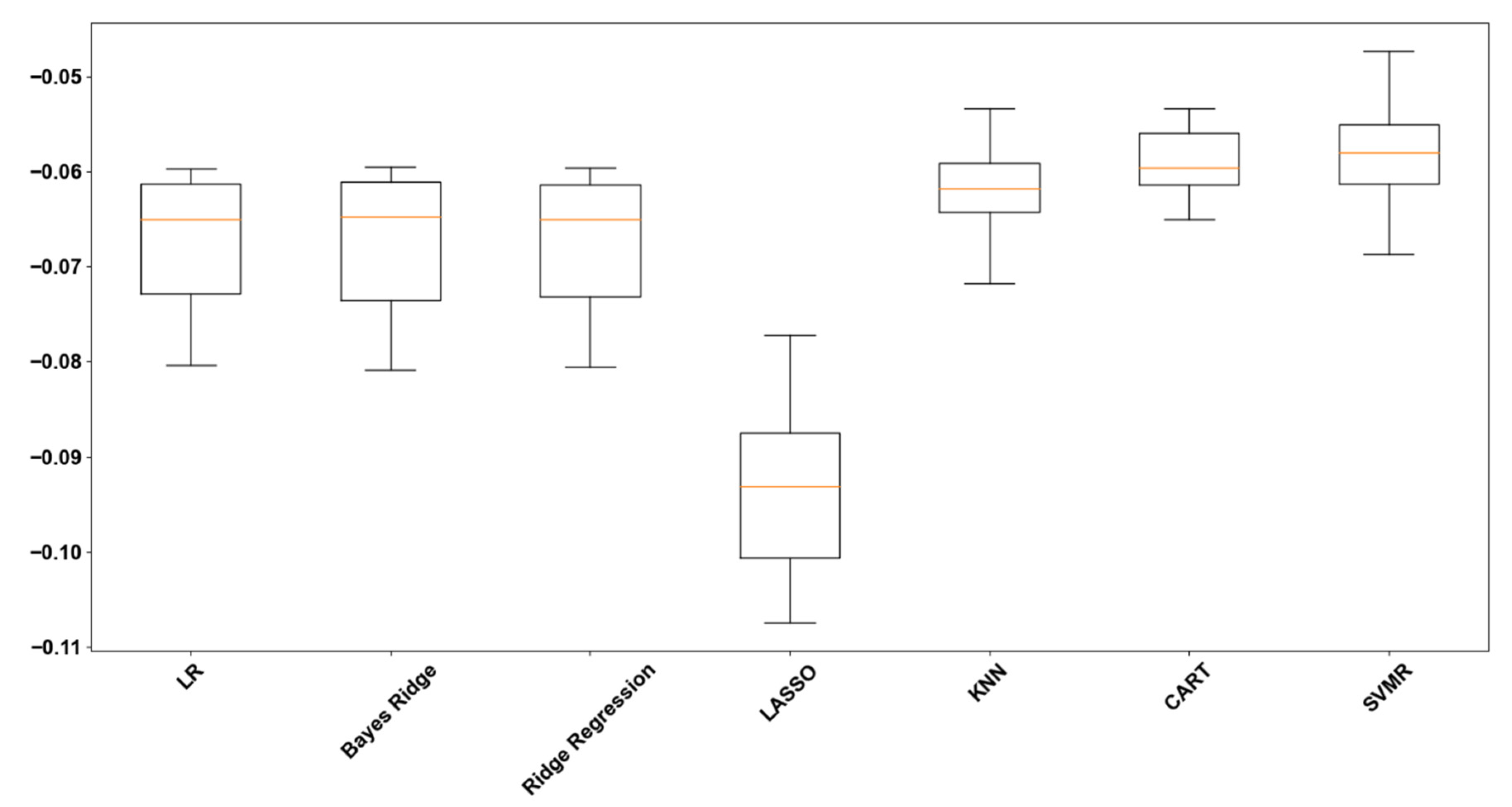
Figure 2.
ML algorithms sensitivity analysis on cross-validation.

Figure 3.
ML algorithms sensitivity analysis on repeated cross-validation.

Figure 4.
Correlation between LOOCV and RCV for all algorithms.
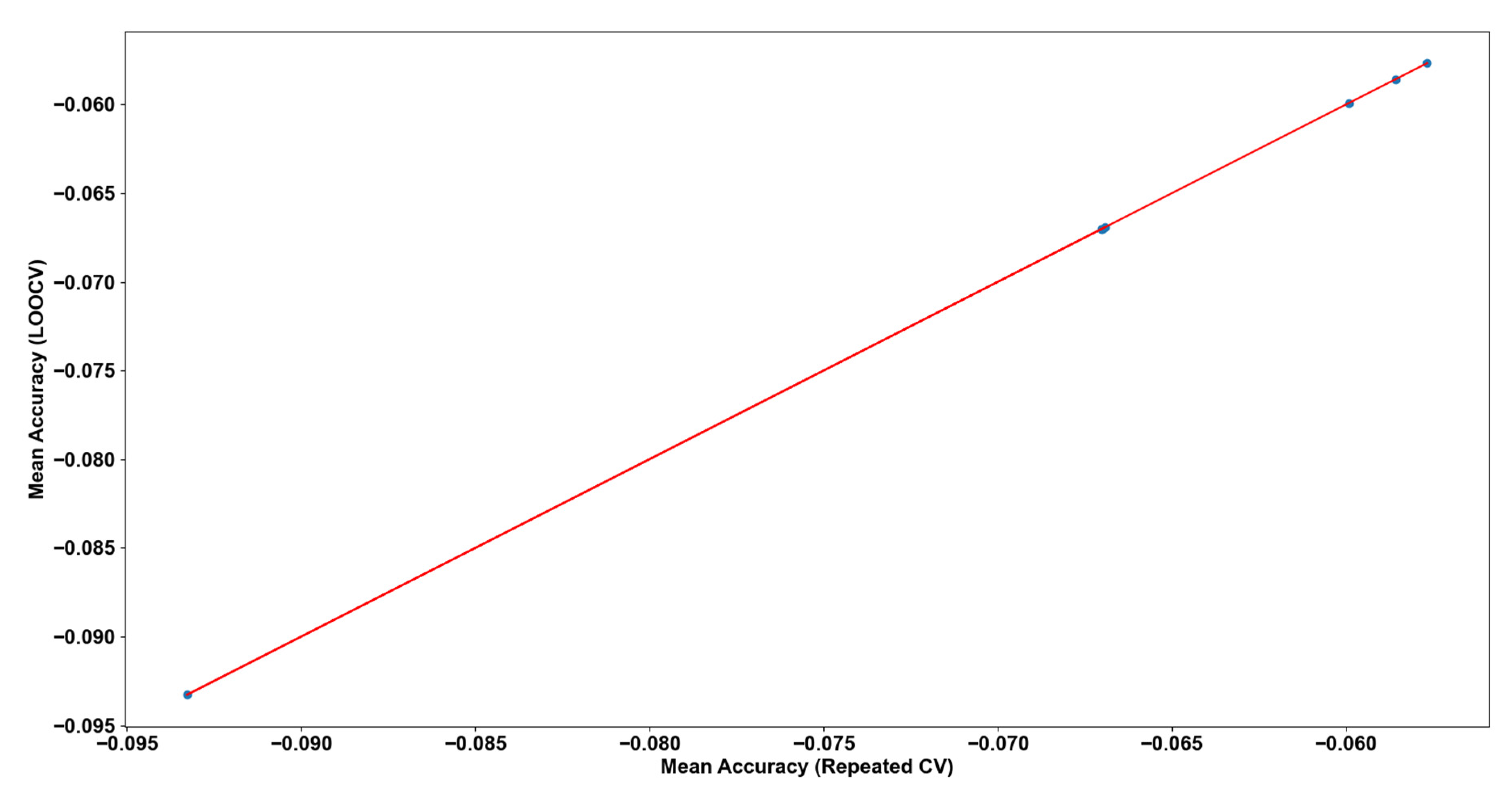
Figure 5.
ML algorithms accuracy scores after optimized RCV.
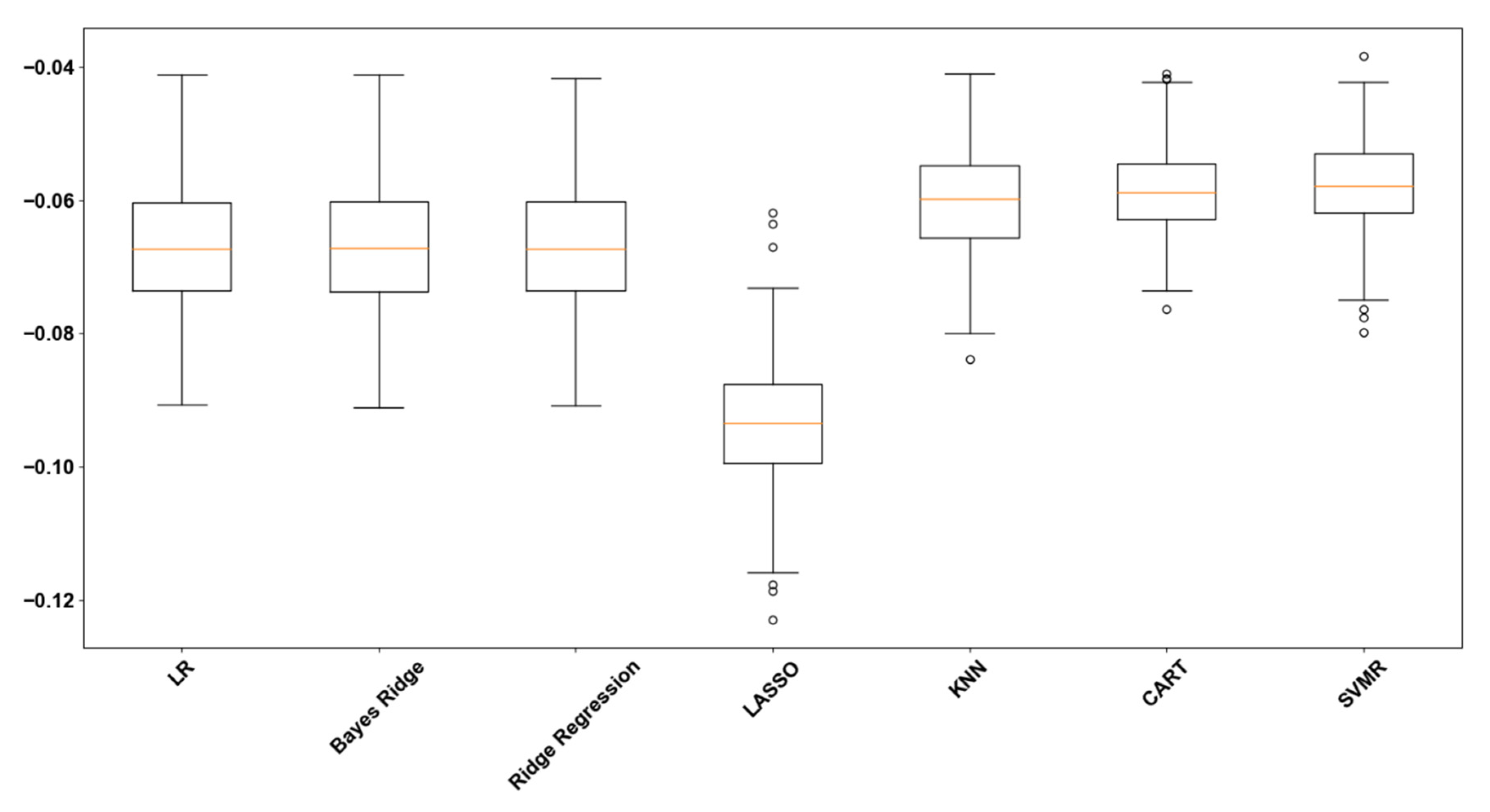

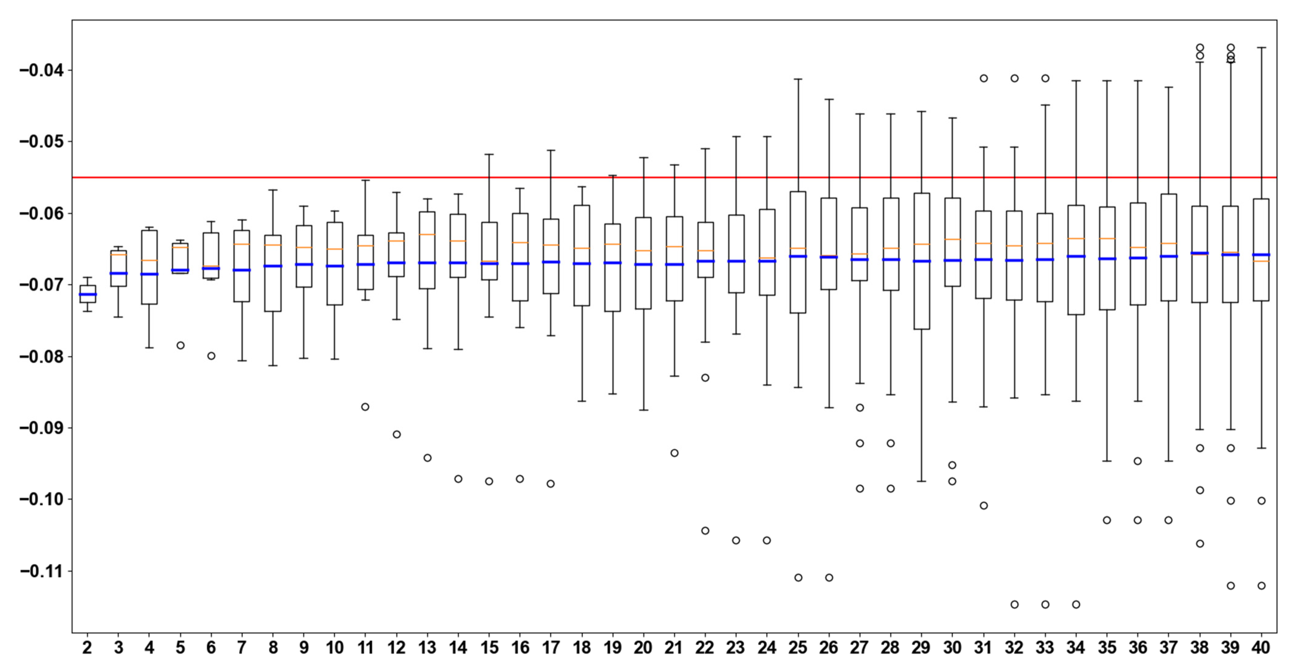
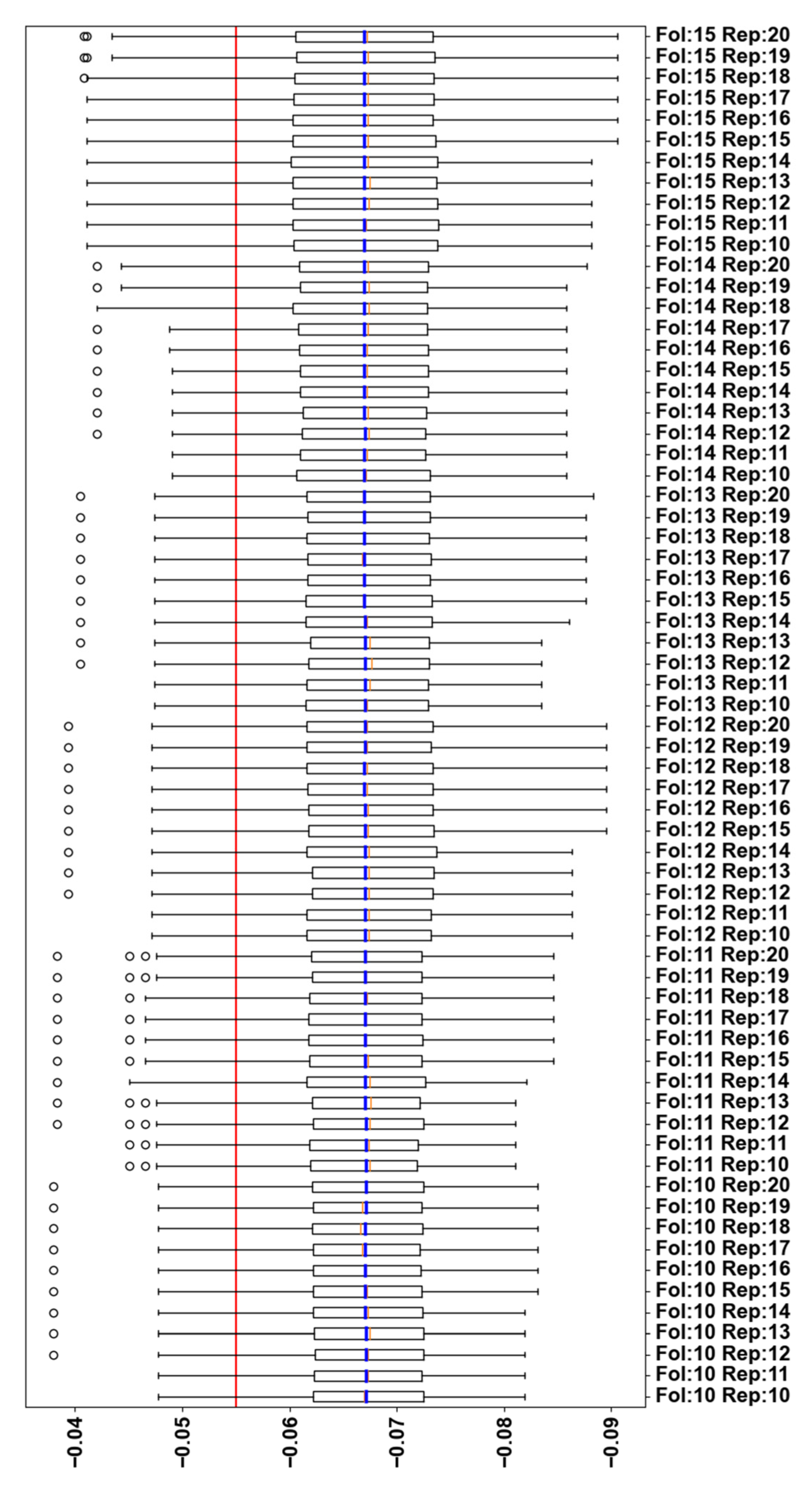
Table 1.
ML algorithms default training and testing.
| ML Algorithm | R2 Train Score | R2 Test Score | RMSE Test Score |
|---|---|---|---|
| Linear Regression | 0.5470 | 0.4754 | 0.00432 |
| Bayes Ridge Regression | 0.54686 | 0.47553 | 0.00432 |
| Ridge Regression | 0.54698 | 0.47548 | 0.00432 |
| LASSO Regression | 0 | −0.0016 | 0.00825 |
| K-Nearest Neighbors | 0.66823 | 0.39674 | 0.00497 |
| CART | 0.8056 | 0.51325 | 0.00401 |
| Support Vector Machines Regression | 0.64731 | 0.56272 | 0.0036 |
Table 2.
ML algorithms training and testing after stratified splitting.
| ML Algorithm | R2 Train Score | R2 Test Score | RMSE Test Score |
|---|---|---|---|
| Linear Regression | 0.49999 | 0.60878 | 0.00362 |
| Bayes Ridge Regression | 0.49978 | 0.60663 | 0.00364 |
| Ridge Regression | 0.49997 | 0.60816 | 0.00363 |
| LASSO Regression | 0.64847 | −0.0014 | 0.00927 |
| K-Nearest Neighbors | 0.6485 | 0.42249 | 0.00535 |
| CART | 0.79909 | 0.58683 | 0.00382 |
| Support Vector Machines Regression | 0.60912 | 0.62566 | 0.00347 |
Table 3.
Correlation of features.
| Management.M1 | Soil_Type.CL | Soil_Type.SL | Precipitation | Relative_Irrigation | Number_of_Trips_Reduction | |
|---|---|---|---|---|---|---|
| management.M1 | --- | 7.071077 ×10⁻¹ | 2.272757 × 10⁻¹⁶ | 1.029597 × 10⁻¹⁶ | 1.007215 × 10⁻¹⁶ | 9.568540 × 10⁻¹⁷ |
| soil_type.CL | --- | --- | 5 × 10⁻¹ | 1.724138 × 10⁻¹⁶ | 5.771856 × 10⁻¹⁶ | 2.890379 × 10⁻¹⁶ |
| soil_type.SL | --- | --- | --- | 4.659030 × 10⁻¹⁷ | 4.062555 × 10⁻¹⁶ | 4.985459 × 10⁻¹⁷ |
| precipitation | --- | --- | --- | --- | 3.69276 × 10⁻¹⁷ | 2.604227 × 10⁻¹⁷ |
| relative_irrigation | --- | --- | --- | --- | --- | 8.9092 × 10⁻¹⁸ |
| number_of_trips_reduction | --- | --- | --- | --- | --- | --- |
Table 4.
ML algorithms training and testing after correlated features exclusion.
| ML Algorithm | R2 Train Score | R2 Test Score | RMSE Test Score |
|---|---|---|---|
| Linear Regression | 0.47358 | 0.58799 | 0.00381 |
| Bayes Ridge Regression | 0.47341 | 0.58531 | 0.00384 |
| Ridge Regression | 0.47357 | 0.58718 | 0.00382 |
| LASSO Regression | 0 | −0.0014 | 0.00927 |
| K-Nearest Neighbors | 0.64755 | 0.41146 | 0.00545 |
| CART | 0.79909 | 0.58683 | 0.00382 |
| Support Vector Machines Regression | 0.60679 | 0.62352 | 0.00349 |
Table 5.
ML algorithms training and testing with transforms application.
| ML Algorithm | R2 Train Score/R2 Test Score | RMSE Score | ||||
|---|---|---|---|---|---|---|
| Scaling | Standardi Zation | Power Transform | Scaling | Standardi Zation | Power Transform | |
| Linear Regression | 0.49999/0.60878 | 0.49999/0.60878 | 0.49615/0.61141 | 0.00362 | 0.00362 | 0.0036 |
| Bayes Ridge Regression | 0.49971/0.60841 | 0.498789/0.60872 | 0.49579/0.61105 | 0.00363 | 0.00362 | 0.0036 |
| Ridge Regression | 0.49998/0.60878 | 0.49999/0.60885 | 0.49613/0.61141 | 0.00362 | 0.00362 | 0.0036 |
| LASSO Regression | 0/−0.0014 | 0/−0.0014 | 0/−0.0014 | 0.00927 | 0.00927 | 0.00927 |
| K-Nearest Neighbors | 0.74781/0.62416 | 0.72762/0.66027 | 0.71500/0.55056 | 0.00348 | 0.00315 | 0.00416 |
| CART | 0.79909/0.58683 | 0.79909/0.58683 | 0.79909/0.58683 | 0.00382 | 0.00382 | 0.00382 |
| Support Vector Machines Regression | 0.63347/0.65531 | 0.63978/0.66826 | 0.63010/0.64965 | 0.00319 | 0.00307 | 0.00324 |
Table 6.
ML algorithms performance scores after optimized RCV.
| ML Algorithm | Mean Accuracy—(Standard Error) For Repeated Cross-Validation after Sensitivity Analysis |
|---|---|
| Linear Regression | 0.066925—(0.008849) |
| Bayes Ridge Regression | 0.067004—(0.008873) |
| Ridge Regression | 0.067029—(0.008846) |
| LASSO Regression | 0.093284—(0.010321) |
| K-Nearest Neighbors | 0.059908—(0.007890) |
| CART | 0.058579—(0.006713) |
| Support Vector Machines Regression | 0.057669—(0.006979) |
Table 7.
SVMR performance before and after tuning.
| R2 Training Score | R2 Test Score | RMSE Test Score | |
|---|---|---|---|
| SVMR—Default hyperparameters | 0.63978 | 0.66826 | 0.00307 |
| SVMR—Tuned hyperparameters | 0.63961 | 0.66833 | 0.00307 |
Table 8.
Ensemble methods mean accuracy scores with RCV.
| Ensemble Method | Mean Accuracy—(Standard Error) For Repeated Cross-Validation |
|---|---|
| Extreme Gradient Boosting | 0.057299—(0.0066) |
| Gradient Boosting | 0.050332—(0.005987) |
| Random Forests | 0.056302—(0.006642) |
| Extra Trees | 0.058541—(0.006728) |
Table 9.
Ensemble methods and Tuned GB. Training and Testing scores.
| Ensemble Method | R2 Training Score | R2 Test Score | RMSE Test Score |
|---|---|---|---|
| Extreme Gradient Boosting | 0.79745 | 0.62404 | 0.00348 |
| Gradient Boosting | 0.77405 | 0.73282 | 0.00247 |
| Gradient Boosting (Tuned) | 0.74533 | 0.72741 | 0.00252 |
| Random Forests | 0.7971 | 0.62462 | 0.00348 |
| Extra Trees | 0.79909 | 0.58924 | 0.0038 |
Table 10.
Observations of improvement for experiments sequence.
| R2 Training Score | R2 Test Score | RMSE Test Score | |
|---|---|---|---|
| Support Vector Machines Regression (Experiment 1) | 0.64731 | 0.56272 | 0.0036 |
| Gradient Boosting (Experiment 9) | 0.74533 | 0.72741 | 0.00252 |
| Performance improvement on the test set (%) | 29.27% | 42.88% |
Publisher’s Note: MDPI stays neutral with regard to jurisdictional claims in published maps and institutional affiliations. |
© 2021 by the authors. Licensee MDPI, Basel, Switzerland. This article is an open access article distributed under the terms and conditions of the Creative Commons Attribution (CC BY) license (https://creativecommons.org/licenses/by/4.0/).
Share and Cite
MDPI and ACS Style
Christias, P.; Mocanu, M. A Machine Learning Framework for Olive Farms Profit Prediction. Water 2021, 13, 3461. https://doi.org/10.3390/w13233461
AMA Style
Christias P, Mocanu M. A Machine Learning Framework for Olive Farms Profit Prediction. Water. 2021; 13(23):3461. https://doi.org/10.3390/w13233461
Chicago/Turabian StyleChristias, Panagiotis, and Mariana Mocanu. 2021. "A Machine Learning Framework for Olive Farms Profit Prediction" Water 13, no. 23: 3461. https://doi.org/10.3390/w13233461
Note that from the first issue of 2016, this journal uses article numbers instead of page numbers. See further details here.