
Simulation-Optimization Model for Conjunctive Management of Surface Water and Groundwater for Agricultural Use


Department of Civil and Environmental Engineering, Dongguk University, Seoul 04620, Korea
*
Author to whom correspondence should be addressed.
Water 2021, 13(23), 3444; https://doi.org/10.3390/w13233444
Submission received: 10 November 2021
/
Revised: 26 November 2021
/
Accepted: 1 December 2021
/
Published: 4 December 2021
(This article belongs to the Section Water Resources Management, Policy and Governance)
Abstract
:The conjunctive management of surface water and groundwater resources is essential to sustainably manage water resources. The target study is the Osan watershed, in which approximately 60–70% of rainfall occurs during the summer monsoon in Central South Korea. Surface water resources are overexploited six times as much as groundwater resources in this region, leading to increasing pressure to satisfy the region’s growing agricultural water demand. Therefore, a simulation-optimization (S-O) model at the sub-basin scale is required to optimize water resource allocation in the Osan watershed. An S-O model based on an artificial neural network (ANN) model coupled with Jaya algorithm optimization (JA) was used to determine the yearly conjunctive supply of agricultural water. The objective was to minimize the water deficit in the watershed subject to constraints on the cumulative drawdown in each subarea. The ANN model could predict the behaviour of the groundwater level and facilitate decision making. The S-O model could minimize the water deficit by approximately 80% in response to the gross water demand, thereby proving to be suitable for a conjunctive management model for water resource management and planning.
1. Introduction
The recent decade has witnessed significant challenges in the sustainable management of agricultural water resources, namely growing water demand, overexploitation of single extraction sources and unrestricted extractions. Surface water and groundwater are the primary water sources for agricultural, domestic, and industrial purposes [1]. An increase in the demand of water for agricultural, domestic, and industrial use necessitates the formulation of alternative water management strategies to mitigate these challenges [2]. Notably, there is a considerable demand for agriculture water, representing approximately 70% of all water consumption worldwide [3]. Agriculture consumed 15.9 billion (m3) of water in 2007, accounting for around 48% of the Republic of Korea’s total annual water usage [4,5]. Moreover, it was reported that by 2020, water scarcity would reach more than 4.4 billion m3 [6,7]. According to a report of the Comprehensive Water Resources Plan (Water Vision 2020), the agricultural water demand in South Korea is significant, with paddy rice water demand accounting for 34.5% (12.90 Gm3/y) of the total freshwater resources (37.35 Gm3/y) in 2011 [8,9]. To satisfy future agricultural water demands, the conjunctive use of surface and groundwater management approaches will be necessary, as agricultural surface water extractions in the Osan watershed are nearly six times higher than agricultural groundwater withdrawals.
In general, the conjunctive use of ground and surface water is a viable alternative to mitigate water allocation problems [10,11]. The conjunctive use practice is based on the distribution of surface and groundwater to consumers via qualitative and quantitative criteria considering system limitations such as constraints associated with economic and social aspects [12,13]. The implementation of the conjunctive use method in managing surface water and groundwater can help not only alleviate water scarcity issues, but also increase the efficiency of water use and enhance the environmental conditions in the irrigated regions [14,15,16,17]. In conjunctive management, a simulation-optimization (S-O) model must be employed to evaluate the relationship between surface water and groundwater resources to achieve a suitable response of aquifers to formulate various water use policies, and thus, efficient water management policies, taking into account the managerial and hydraulic properties in the region [18]. Physical simulators primarily use traditional equations to model surface water and groundwater when forecasting the groundwater level. However, this method may lead to unsatisfactory forecasts owing to the inaccurate parameter tuning techniques. Recently, data-based simulators, such as those involving artificial neural networks (ANN), have become broadly applied owing to their higher accuracy and superior performance. In particular, such models can address the limitations of physical models, as instead of using traditional equations, such models can accurately establish the correlation between the output and inputs [2,19]. In conjunctive water-use strategies, data-based simulations have been combined with optimization models such as the genetic algorithm (GA) to attain optimum water management strategies. A combined framework involving simulation and optimization models is an effective tool for solving water allocation problems [12,20,21].
ANN is a data-driven technique that has been widely used in the hydrology domain in applications ranging from real-time to event-based modelling, as it can model a highly nonlinear process even in the presence of limited data [22,23,24,25,26,27,28,29,30]. In particular, modelling and forecasting of ANNs have been utilized in water quality, rainfall runoff, and precipitation [31]. Notably, ANN models can adjust to recurring variations and recognize trends in a complicated natural process.
In recent years, several researchers have employed simulation and optimization models in the context of irrigated agriculture to plan and optimize conjunctive water usage [2,17,19,32,33,34,35,36,37,38,39,40]. In 2016, ANN and an ant system optimization were used as an S-O model to predict the monthly conjunctive water supply for irrigation in the Zayandehrud River basin in central Iran. The authors indicated that the model could successfully determine a suitable management model with water extraction quantities for the available surface and groundwater and help enhance the aquifer conditions in the watershed [12]. Genetic programming (GP) as a simulator and multi-objective GA (MOGA) as an optimizer were used to minimize the irrigation water demand and maximize the agricultural net benefits for the region’s main crop in the Gavkhouni river basin, Iran. The findings showed that the optimal conjunctive use model, based on the S-O management model, can enhance the net benefits with the fewest negative socio-environmental consequences [2]. Moreover, an integrated S-O model with a water evaluation and planning system (WEAP) model was linked with the nondominated sorting GA II (NSGA-II) optimization algorithm to enhance reservoir operations, water allocations to irrigation canals, and river withdrawals and groundwater drawdowns in the Zayandehrud river basin, Iran. Results showed that the overall sustainability of the optimized model was 26% greater than that previously achieved with only a simulation model. Moreover, the sustainability of the reservoir and aquifers could be increased by 37% and 16%, respectively [41]. However, none of the existing studies have addressed the conjunctive use of surface and groundwater in the watershed considered in this research. This research represents the first attempt to introduce the Jaya algorithm (JA) in water resource management to optimize conjunctive surface and groundwater management. Similar GAs have been successfully used to develop water allocation policies [42,43,44,45].
The aim of the study is to simulate a single optimization model for conjunctive use of stream flow and groundwater for agriculture in the Osan watershed. A trained ANN model was used to consider the variations in the weather condition and uncertainty resulting from climate conditions in an eleven-year period, whereas the JA used the S-O model to optimize surface and groundwater extraction. The ANN model was used as a simulation model, and the JA was used for optimization to minimize water shortages for agriculture in the considered watershed, which is subject to the groundwater level, to solve a water allocation problem.
2. Materials and Methods
2.1. Area of Study
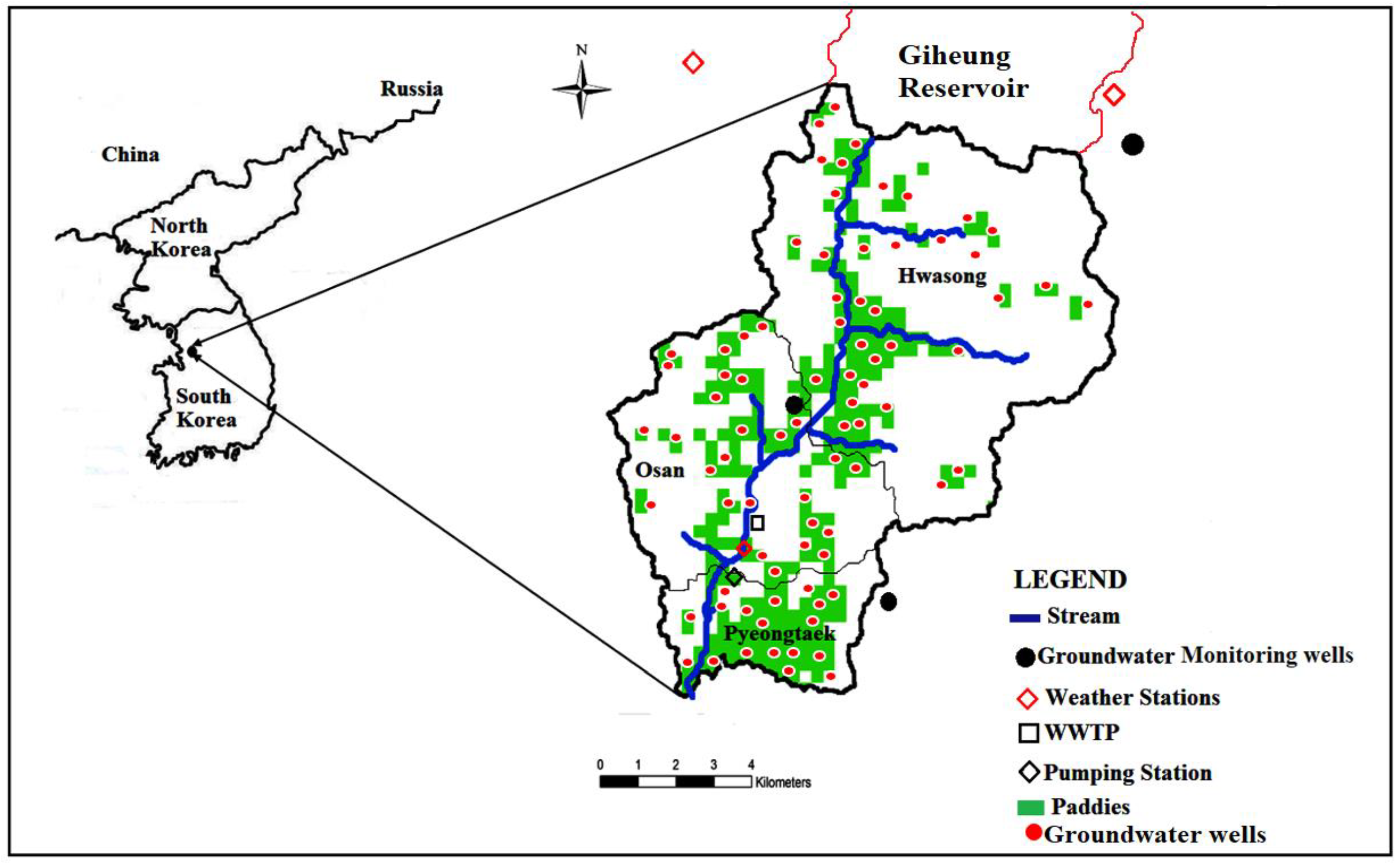
The Osan watershed is a small inland basin in South Korea that lies between latitudes N 37°05′56″ to N 37°14′05″ and longitudes E 127°01′29″ to E 127°09′38″. This watershed has a stream length of 16.49 km and an area of 98.3 km2 (Figure 1). The standard Osan water resource management area starts from the Giheung reservoir and passes through Hwasong city, Osan city, and Pyeongtaek city, which cover the length of the Osan stream. The drainage density of the watershed is 0.52 km/km2, with a drainage slope of 10.21%. The region has a temperate climate with four distinct seasons and a temperature and precipitation of 12 °C and 1321 mm per annum, respectively. The majority of the annual precipitation occurs in the monsoon season (June to September), contributing to approximately 70% of the water availability [7,46,47]. The study area consists of a forest area (32.3%), an urban area (26.1%), paddy rice area (18.3%), barren land (8.1%), upland rice area (6.2%), and grassland and water area (3.5%) [4,46]. The watershed has a wastewater treatment plant with a daily treatment capacity of 140,000 m3. Nearly 1 km downstream, there exists a pumping station where the effluent is poured directly into the stream, and the mixed water is utilized for agriculture.
Meteorological data pertaining to the monthly rainfall and average monthly temperature were collected from the Korean Meteorological Administration (https://data.kma.go.kr/data/grnd/selectAsosRltmList.do?pgmNo=36/ accessed on 8 March 2021). Yearly agricultural groundwater extraction and yearly agricultural surface water supply data were obtained from the Water Resource Management Information System (http://www.wamis.go.kr/ accessed on 3 March 2021), and daily real-time groundwater level data were obtained from the National Groundwater Information Center (http://www.gims.go.kr/ accessed on 10 February 2021).
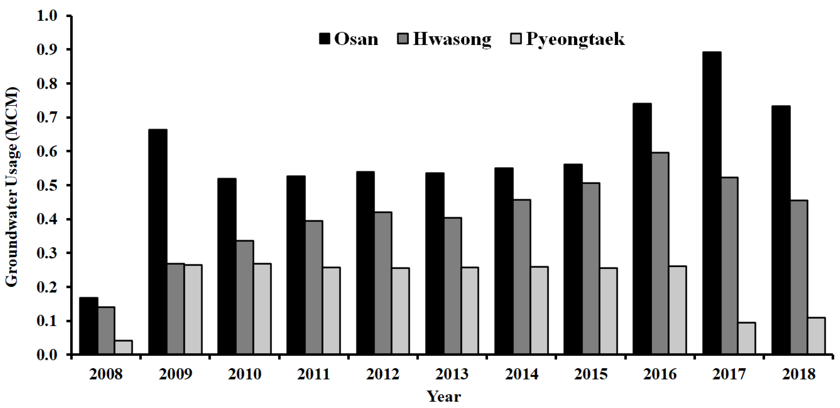
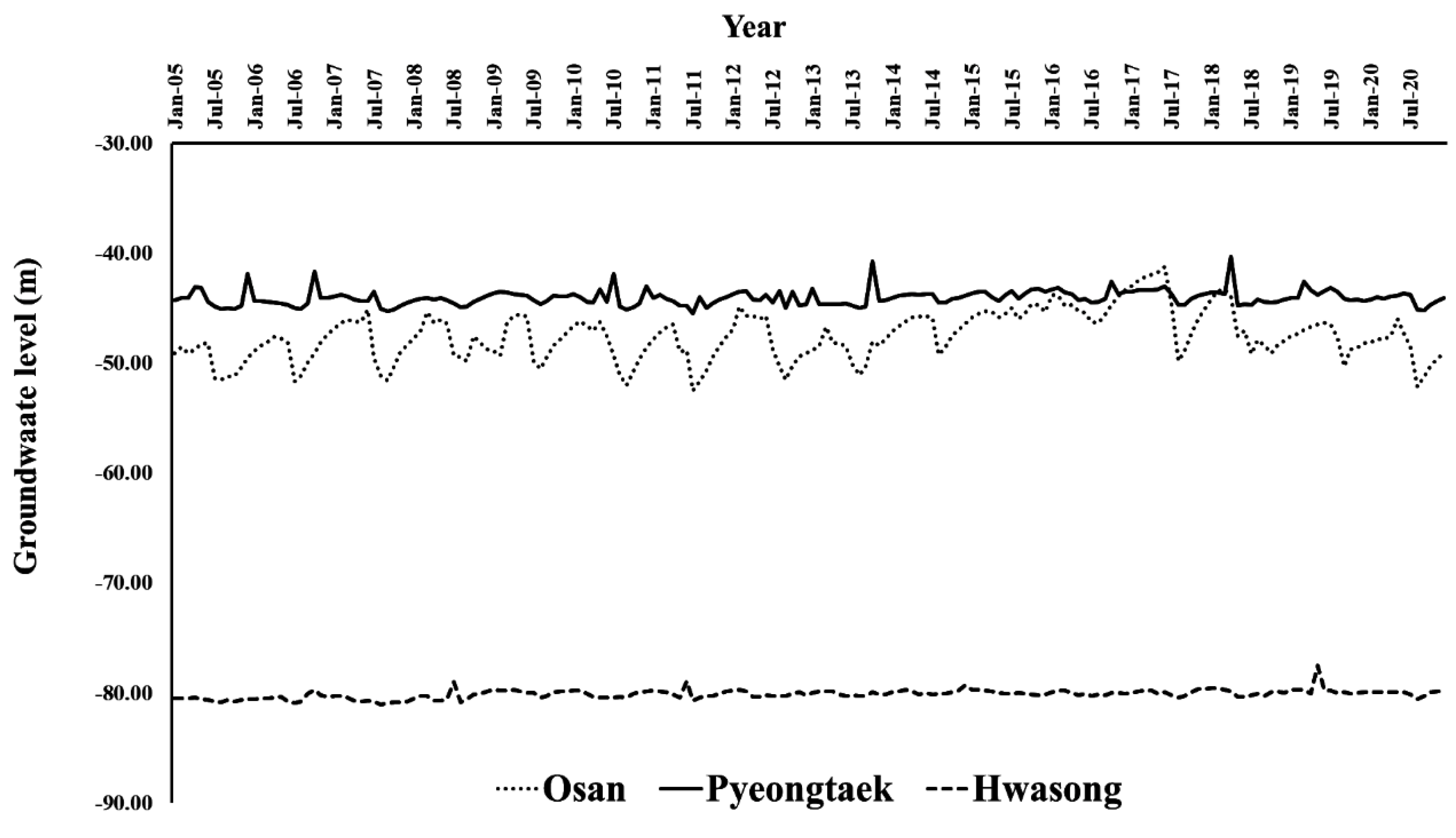
The agricultural surface water extraction in the watershed is supplied by the Osan stream with a farmland of approximately 2408 ha (Figure 2). Figure 3 shows the agricultural groundwater usage, pumped from approximately 155−1160 wells yearly, especially during the dry seasons. During the dry season, groundwater is the main water supply in South Korea [48]. Figure 4 shows the groundwater level for the three subareas in the watershed. The depths of the well range from 20 to 70 m, and hourly real-time data of electric conductivity, water temperature, and water level are provided. Groundwater level problems are expected in the future, as the total annual water resource investments are concentrated on groundwater development in the dry season, and only a small fraction is allocated for groundwater management [49]. Groundwater recharge is not predicted to increase owing to the increased precipitation. The average annual recharge of groundwater in Korea is 12.01% of the total annual precipitation, corresponding to 16.3 billion m3 per year [49,50].
Irrigation is the principal water source for agriculture, as mainly paddy rice is cultivated in the region. The agriculture pattern pertains to single-season planting with mainly summer and autumn harvests. The FAO-CROPWAT model was used to determine the yearly gross water demand in the watershed and the crop water requirement (CWR) of rice per year. CROPWAT is a model used by FAO mainly for irrigation management using soil, crop, and climate data to stimulate irrigation requirements, reference, and crop evapotranspiration [51]. Table 1 summarizes the CWR, water supply, and water demand in the watershed. The water demand equation can be expressed as follows:
Table 1 shows that there is a huge water deficit in the Osan watershed, as the surface and groundwater supply does not meet the water demand calculated by the FAO-CROPWAT model. There is no irrigation system in the watershed, but farmers divert the Osan stream water into their various farms during irrigation periods. Planned irrigation schedules can aid in reducing the water deficit, as the farmers irrigate only when water is needed, as they have different irrigation times. Most farmers own wells on the farms, and they use it in case of stream water shortages.
2.2. ANNs
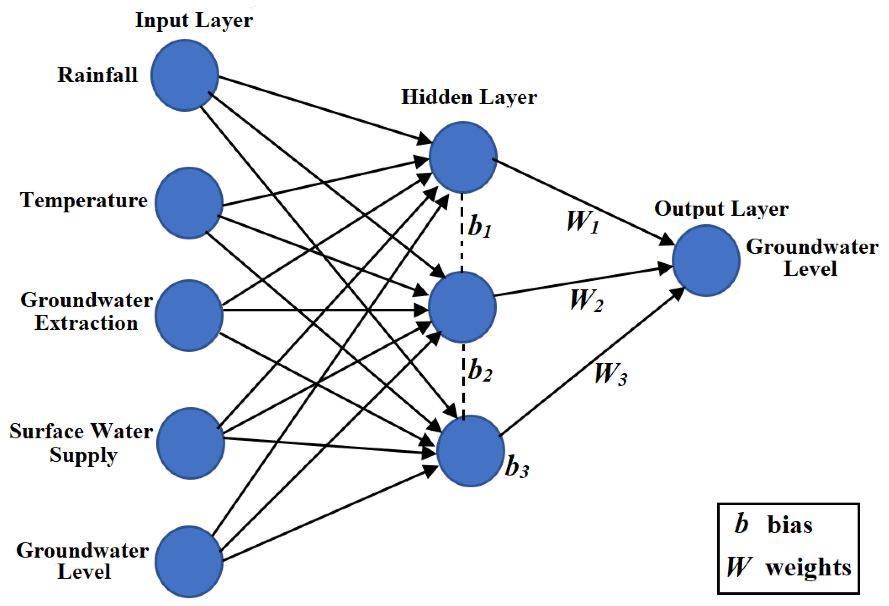
ANNs, as a type of artificial intelligence, aim to mimic the human brain and nervous system. With the use of datasets, ANN models can be trained to create forecasting models and understand the fundamental interactions without using parameters [52]. Several types of ANNs have been used in hydrological modelling [12,53,54,55,56]. An ANN model involves three layers: an input layer, hidden layers with weights and biases, and an output layer (Figure 5).
To conduct simulations based on ANNs, the fundamental concepts of system dynamics must be understood. Therefore, in this study, the groundwater level in the watershed was estimated using models based on annual data. Multilayer perceptron (MLP) ANNs have been widely used to solve hydrological problems [1], especially in combination with the Levenberg–Marquardt algorithm, which renders the model more efficient and stable. Compared to the conventional approaches for simulating the groundwater level, this learning method is more prompt, although it may easily fall into the local minima [57].
In this study, we adopted the Levenberg–Marquardt training technique and a single-layer architecture with three hidden layers by using MATLAB neural network fitting tools. In simulating the groundwater level, a variety of input parameters that directly affect the surface and groundwater interactions were considered. For input data selection, previous studies have used the law of conservation of mass [12,58]. The law states that the groundwater level fluctuates based on aquifer storage variations as a result of surface and groundwater interactions. The factors input to the model included the mean temperature, cumulative groundwater withdrawal for each subarea, precipitation, cumulative surface water allocated for irrigation for each subarea, and initial groundwater level. Runoff and stream water levels were not considered, as they did not directly have an impact on groundwater level. The ANN output was the groundwater level. The ANN network has a 5-60-1 configuration, with the hidden layer consisting of 60 neurons that were generated randomly until the mean square error was achieved. A separate ANN model was prepared for each subarea using specific inputs. In the context of the Osan watershed, the objective was to replicate the ANN model to attain the monthly groundwater levels.
All the data series were split into two sections (65% and 35% for training and testing, respectively), and the ANN performance was evaluated considering the indicators of the coefficient of determination (R2), mean absolute percentage error (MAPE), mean absolute error (MAE), and root mean square error (RMSE), described as in the equations below:
where denotes the observed values, denotes the simulated values, represents the observed mean values, represents the mean simulated values, and represents the number of variables. In general, under ideal conditions, the best match among actual and predicted variable results in an RMSE of 0 and R2 of 1.
2.3. JA
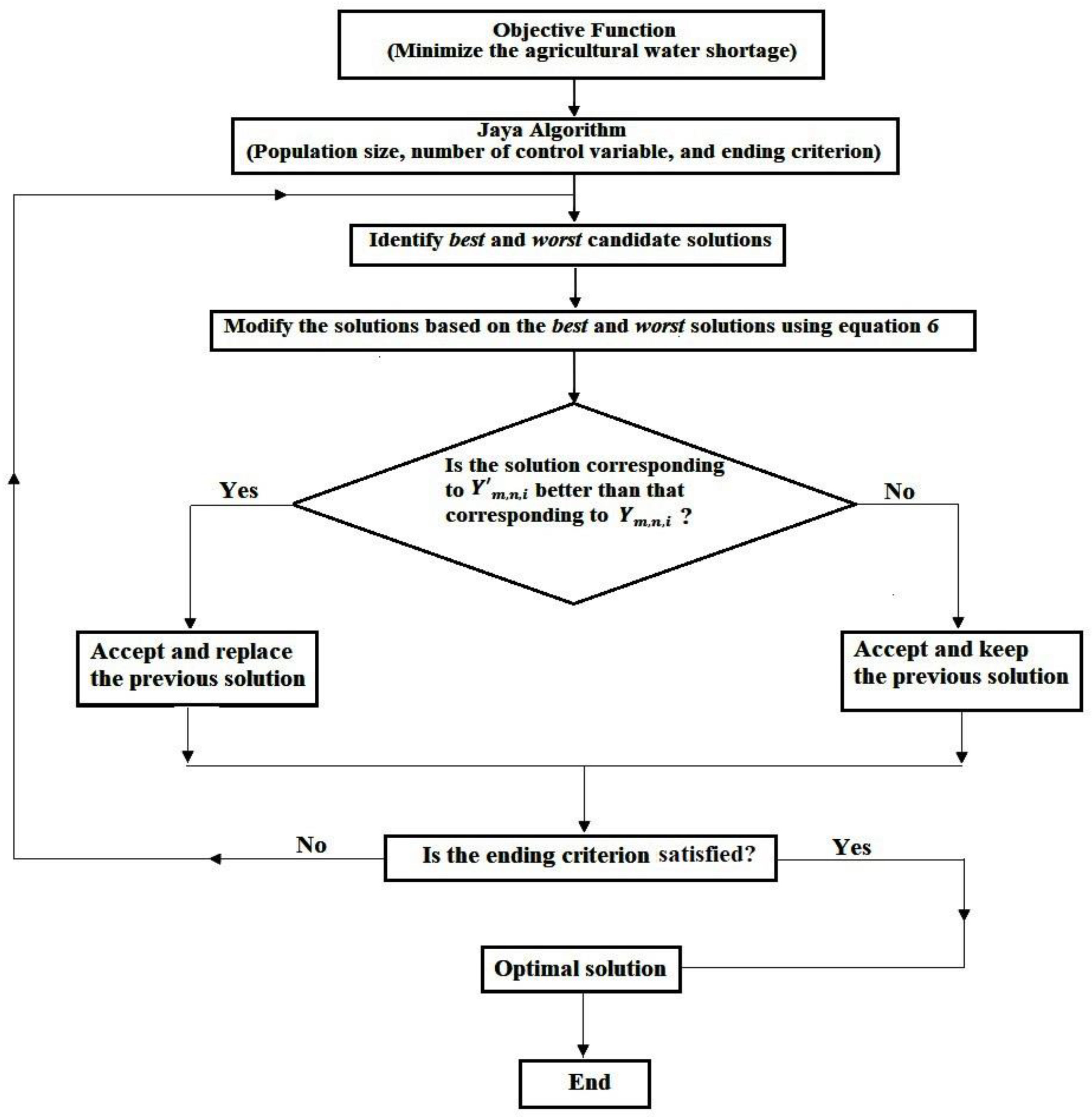
In solving constrained and unconstrained optimization problems, the JA has no algorithm-specific controlling parameter. Compared to similar population-based heuristic algorithms, JA involves only two controlling variables, namely, the number of generations and population size [59]. Moreover, the JA has only one phase, which renders the optimization approach simple. The parameter values can be represented as binary codes to attain a high degree of accuracy. The working principle and theory of JA have been described in existing studies [60,61,62]. The main objective of the JA is to identify the best possible solution for a given problem while avoiding the worst possible outcome.
Let represent the objective function of the JA. For iteration i, j indicates the iterations numbers (m = 1, 2, …, d), and k indicates population size (n = 1, 2, …, e). and Ym,best,i indicate the worst and best candidate solutions, respectively. represents the estimated value of the mth parameter
where and represent the best and worst solutions for the jth parameter, respectively. is the updated value of . Moreover, and are random numbers within [0,1]. The terms “” and “” represent the willingness of the solution to the best and worst solutions, respectively. is adopted if a prior candidate achieves the best solution [59]. The process flow of the JA is shown in Figure 6.
2.4. S-O Model
The objective is to minimize the agricultural water shortage unless the water demand exceeds the total available water. The ANN model outputs are optimized using the JA to attain the best conjunctive management practice subject to various constraints. The objective function is represented as
subject to
where is the demand, and is supply in year i. is the surface water volume supplied (MCM) in year i, is the maximum usable surface water volume in year i, is the extracted groundwater volume in year i, is the maximum volume of groundwater available in year i, is the volume of groundwater level change in year i, and is the maximum volume of groundwater in year i.
To account for the conditions in which the constraints are breached, a penalty function is introduced in the minimization objective function, with representing the penalty coefficient (an exceptionally large positive value), and representing the violation of the acceptable threshold of each constraint. The value of the violation is multiplied by a significance coefficient to determine the penalty. These sanctioned violations are introduced in the problem formulation to help satisfy the minimization objectives. The maximum volume of the available surface water, maximum volume of available groundwater, and maximum volume of groundwater change in year are set as 60 MCM, 5 MCM, and 1.5 m, respectively.
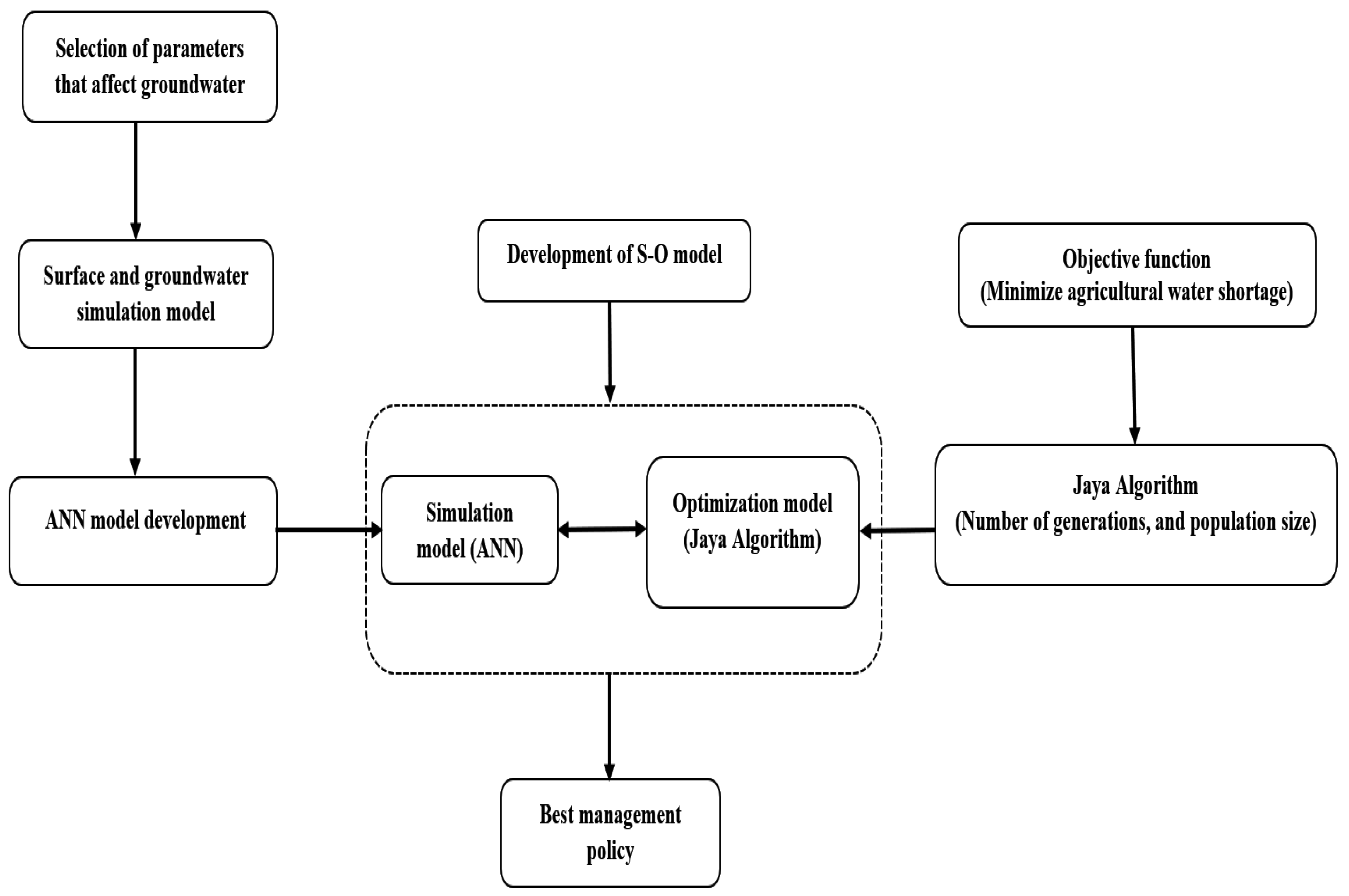
The objective function coupled with the constraint constitutes a nonlinear optimization problem. The ANN model and JA are externally linked to optimize the usage of groundwater and surface water in the watershed considering the groundwater level. In assessing the constraints and objective function, the ANN model and JA were used to simulate the annual groundwater level changes with respect to the quantities of groundwater extraction and surface water allocation in the watershed as decision variables. Figure 2 and Figure 3 show that the surface water resources are limited in the watershed. Consequently, water resource managers must establish suitable policies corresponding to each year’s needs and demands and allocate the usable water resources to meet the future demand of water. Figure 7 illustrates the linkage of the ANN model and JA optimization.
3. Results
3.1. Predictive Capability
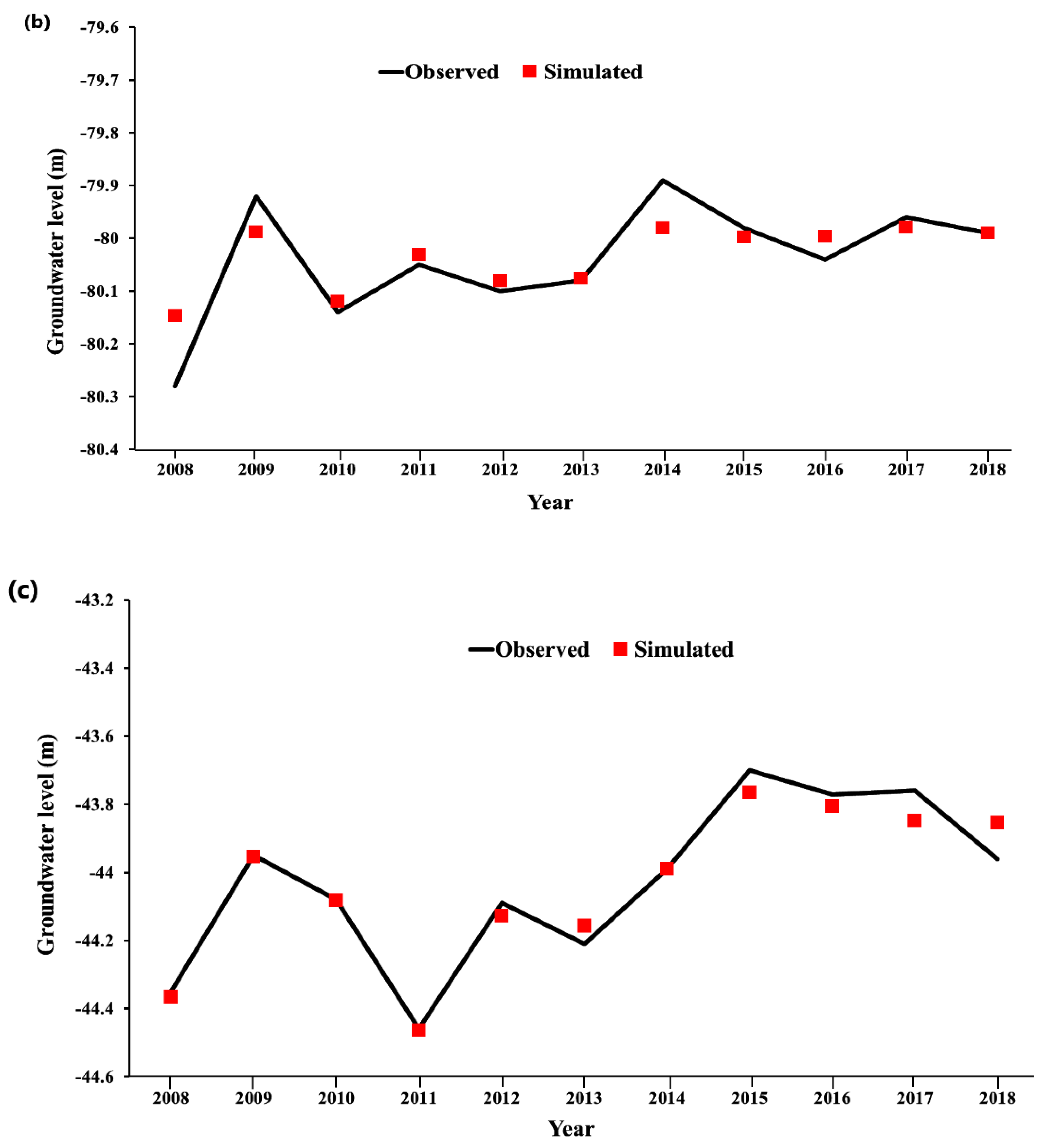
The Osan watershed was used to apply the proposed ANN model, specifically, the Osan, Hwasong, and Pyeongtaek areas. With the help of MATLAB, the optimization toolbox was used to predict groundwater levels in the watershed. Table 2 summarizes the ANN results. The best-fit neural network structures were determined for each subarea depending on the R2, RMSE, MSE, and MAPE values. Their respective values were 0.92, 0.12, 0.02 and 0.15 for the Osan subarea, 0.81, 0.01, 0 and 0.01 for the Hwasong subarea, and 0.98, 0.02, 0 and 0.08 for the Pyeongtaek subarea. The performance indicators were satisfactory in the training and testing of the ANN simulation model.
Figure 8a–c shows the ANN model results for each subarea, along with a comparison of the mean values of the observed and simulated groundwater level. The input parameters, namely, the temperature, rainfall, surface water supplied, groundwater extraction, and initial groundwater level most considerably influenced the groundwater level in the Osan watershed.
3.2. Optimal Conjunctive Use
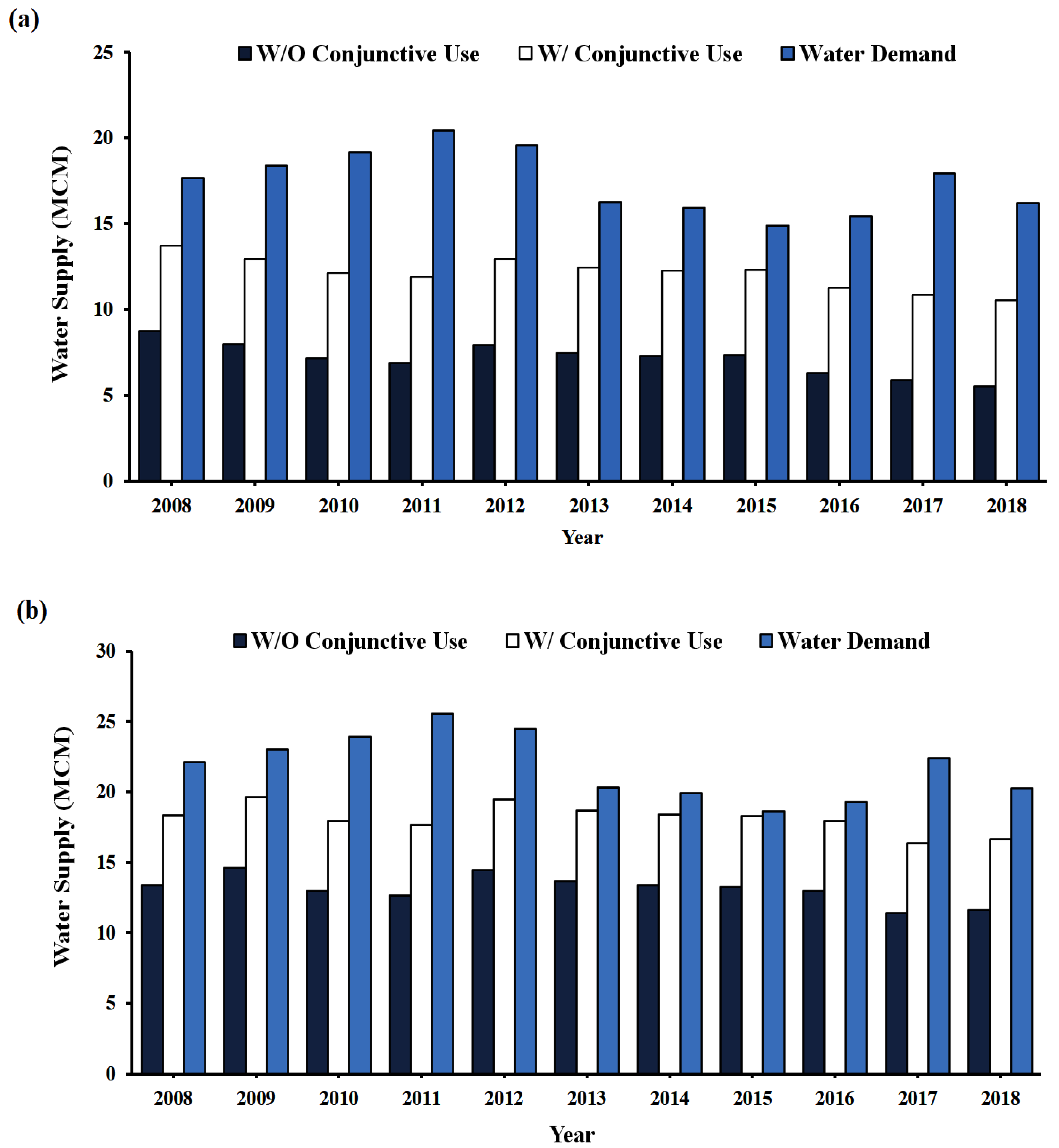
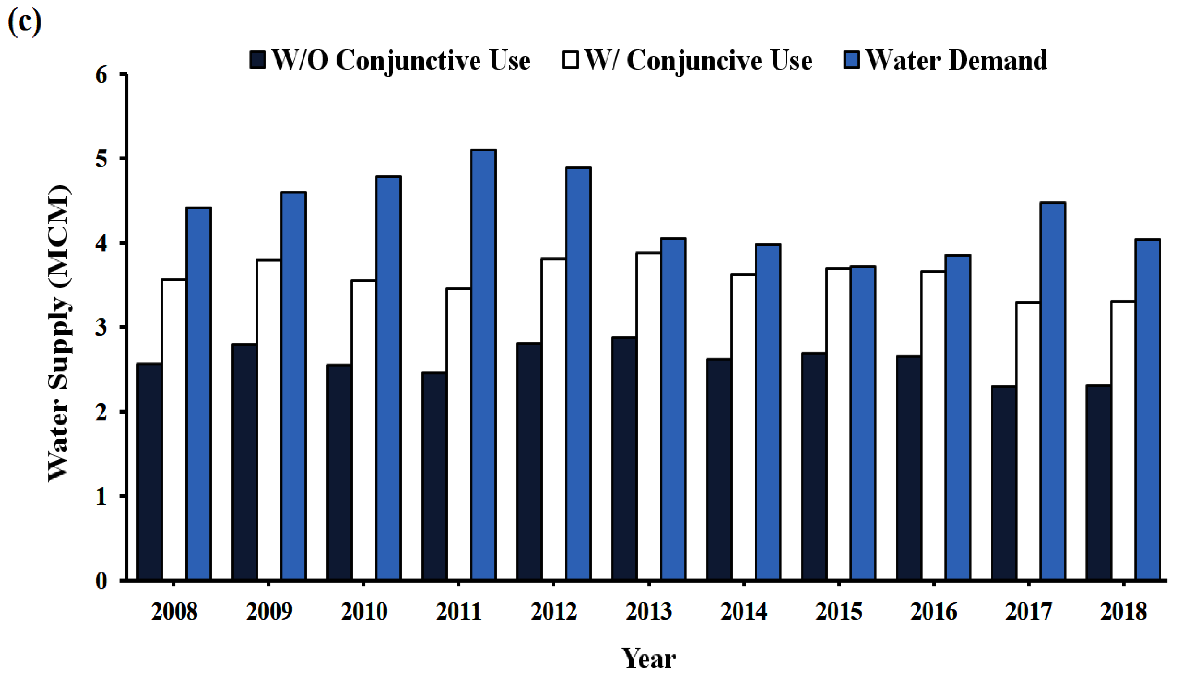
Figure 9 displays the S-O model’s results for total water usage in the Osan watershed. These diagrams show the amounts of water supplied with and without conjunctive use in the subareas in the Osan watershed. Comparison of Figure 9a–c indicates that with conjunctive management, water temporal distribution was improved, thus minimising water deficiency with respect to the water demand. Figure 9a shows that in the Osan subarea, there was an increase in water supply, which met approximately 40% of the water demand without conjunctive use in Osan, as compared to meeting about 70% of water demand with conjunctive use. A similar pattern was seen in Figure 9b, as the amount of water supply increased from about 60% without conjunctive use to approximately 83% with conjunctive use in the Hwasong subarea. Furthermore, Figure 9c also indicates an increase of water supply from 60% without conjunctive use to 83% with conjunctive use in the Pyeongtaek subarea.
Table 3 summarizes the distribution total water supply and water deficit with and without conjunctive use in the Osan watershed. The water deficit is specified with respect to the water demand pertaining to the crop water requirement in each subarea, calculated using the FAO-CROPWAT model defined in Equation (1). In the Osan subarea, the total water supply ranges from 5.52–8.74 MCM with a deficit of 7.57–13.53 MCM without conjunctive use. With conjunctive use, the total water supply increased to 10.52–13.74 MCM and the deficit decreased to 2.57–8.53 MCM. In the Hwasong subarea, the total water supply and deficit was 11.38–14.62 MCM and 5.36–11.01 MCM, respectively, without conjunctive use. The Hwasong subarea shows a similar pattern, as total water supply increased by 16.38–19.62 MCM, whereas the water deficit reduced by 1.36–7.87 MCM. In the Pyeongtaek subarea, without conjunctive use, the total water supply was 2.30–2.88 MCM and deficit was 1.03–2.65 MCM. With conjunctive use, there was an increase in the total water supply of 3.30–3.88 MCM, and the deficit decreased by 0.03–1.65 MCM. From these results, conjunctive use increases water supply and decreases deficit throughout the Osan watershed.
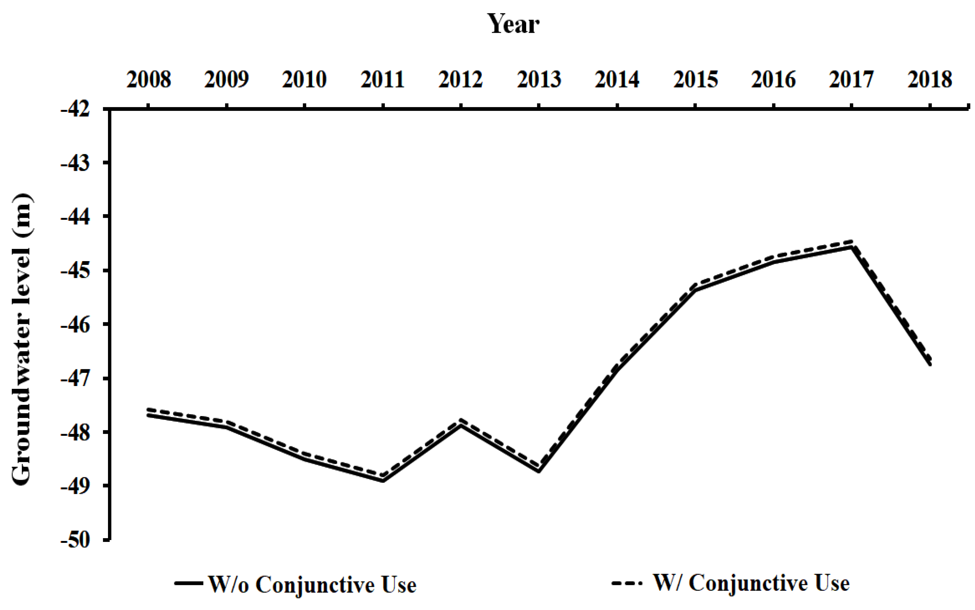
The groundwater level in the cases with and without conjunctive use in the Osan subarea are comparable. Figure 10 shows only the change in the groundwater level for the Osan subarea, owing to the similar pattern observed for the three subareas (no change in the temporal distribution of water). This phenomenon can likely be attributed to annual water recharge, which occurs during the summer monsoon season with an annual rainfall of 1321 mm. Besides precipitation during the summer monsoon, irrigation water for rice paddies increases groundwater levels as a result of water flow back [63].
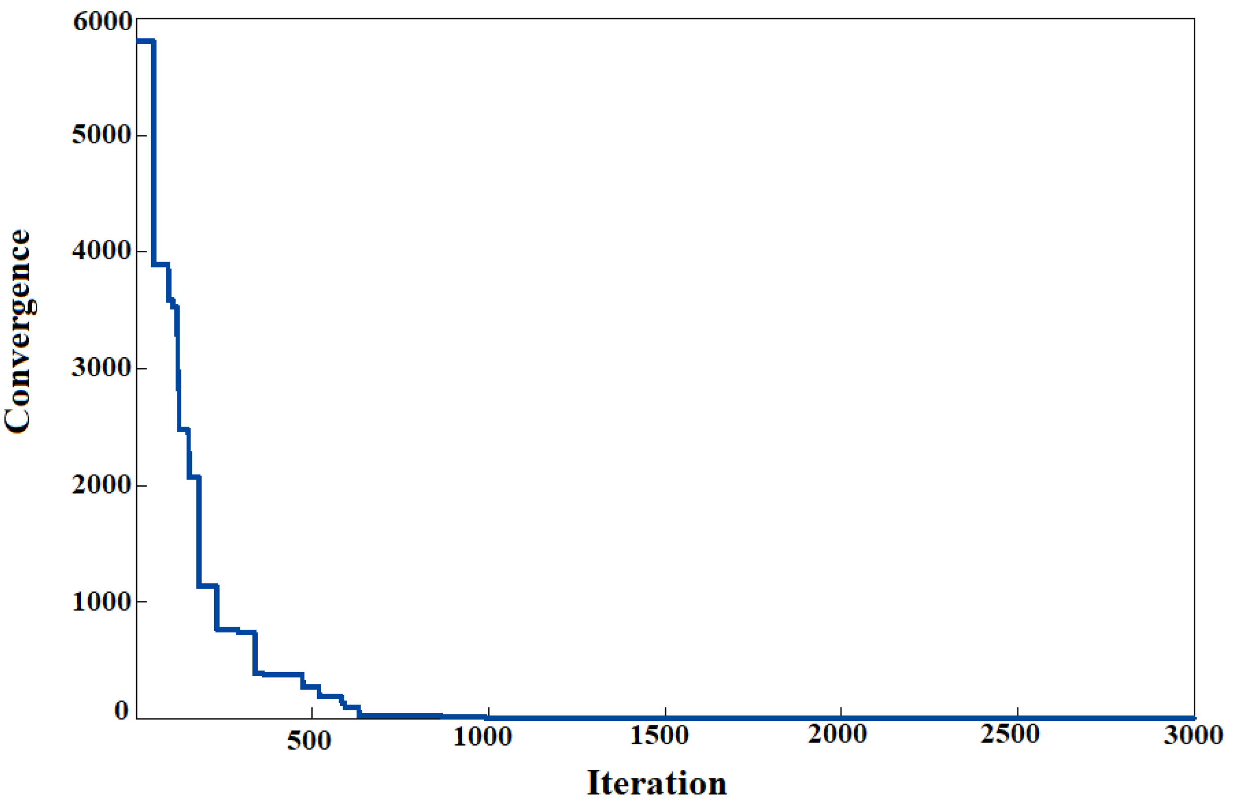
Figure 11 shows that the curve converges to an optimal point after 500 iterations for the JA. The optimization objective is satisfied, attaining a reasonable solution in 3000 iterations, corresponding to maximum convergence.
The single objective optimization model used in the study corresponds to the best possible solution to the water shortage minimization problem when using the S-O linked model with conjunctive use of the surface and groundwater resources in the Osan watershed.
4. Discussion
The accuracy of the ANN model from 2008–2018, as shown in Figure 8, indicates that the groundwater level was successfully predicted in each subarea and could be used to facilitate water management decision-making. The values indicated that ANN learning exhibits a reasonable precision, and the values for the testing and training stages indicate that overtraining does not occur. The ANN model performance was validated by these statistical metrics (Table 2).
The S-O model was applied to the Osan watershed to minimize water shortages. Groundwater is extracted mostly when surface water shortages occur to compensate for this shortage and satisfy the agricultural water demand in this region. Even though water is not generated in conjunctive management, water can be efficiently distributed, thereby minimizing the water shortage [12,64]. In other words, conjunctive water management can control the amount of groundwater extraction when allocating the surface water. Moreover, the S-O model can alter the distribution of the available surface and groundwater quantities to satisfy the agricultural water demand and reduce water shortage in the Osan watershed (Figure 9). The results are in accordance with other similar studies on S-O models, as conjunctive use reduces water shortage and reduces water demand [2,12].
Yearly water allocation and water demand from 2008 to 2018 are presented in Table 1. Clearly, the available supply is insufficient to meet the gross water demand necessary to realize the full agricultural potential. The S-O model can enhance the temporal water distribution in the region and optimize the water demands under the given constraints with respect to the crop water requirements. Although the water supply in the S-O model is increased, it cannot satisfy the agricultural water demand. Conjunctive water management can clearly enhance the water supply, and other aspects such as crop diversification and agricultural water demand can be satisfied, as paddy rice is the main water consumer in the region, owing to the considerable water consumption in rice cultivation. In general, water shortage minimization problems are designed to optimize the distribution of surface water and groundwater to reduce the overexploitation of either water source.
Although Table 1 presents the gross water demand for the Osan watershed, we also presented the individual water demand for each subarea to visualize how conjunctive use affects the surface water and groundwater distributions. When conjunctive use is applied, the total water supply increases, which reduces the deficit with respect to the water demand in the watershed. The total water supply can reach approximately 80% of the water demand in the Osan watershed. The cultivation of a smaller area and use of crop rotation techniques can help satisfy the water demands [12].
Overall, the best solution for the water shortage optimization problem were achieved by employing the S-O model of the conjunctive use of surface and groundwater using a single-objective optimization. This S-O model is capable of controlling the surface and groundwater balances in the Osan watershed.
5. Conclusions
An S-O linked model was created to enable the conjunctive use of surface water and groundwater resources to minimize water shortages for agriculture in the Osan watershed. An ANN was used as the simulation model, and the JA was used as the optimization model. The ANN model had a single-layer architecture with Marquardt training implemented. The output of the hidden layer has a linear function capable of predicting the groundwater level. The model input parameters were the groundwater extraction, surface water supply, temperature, rainfall, and initial groundwater level. The output results were provided to the JA to optimize water resources usage in the Osan watershed. The ANN model was capable of predicting groundwater level in the study and can be used as a decision support system in future research.
The S-O model was aimed at reallocating the surface water and groundwater portions, as the surface water extraction was six times higher than that for the groundwater resources; therefore, the S-O model aimed at reducing the difference in the supply and demand of water in the watershed subject to constraints attributed to the maximum allowable surface water supplied and groundwater extracted. Our research is the first attempt to introduce the Jaya algorithm (JA) in water resource management to optimize conjunctive surface and groundwater management. According to the S-O model results, the potential water supply in the Osan watershed cannot meet the agricultural water demand. However, the framework could minimize the water shortage to enhance water efficiency with negligible water drawdowns while satisfying approximately 80% of the water demand. It is necessary that farmers should maximize their farmland by using crop rotation techniques and planned irrigation schedules, which can help in satisfying the agricultural water demands in the Osan watershed. Overall, the performance of the conjunctive use of surface and groundwater was satisfactory. The proposed S-O model can aid in water resource management and planning (groundwater and surface water). This framework can promote the development of optimal management practices for the conjunctive management of groundwater and surface water resources, thereby facilitating decision making for water resource managers.
Further research on forecasting several years for the conjunctive management of surface and groundwater under different scenarios with constraints to climate change will improve the water resource management in the region.
Author Contributions
A.B.A. and S.-I.L. developed the methodology and prepared the manuscript. A.B.A. conducted the research under the supervision of S.-I.L. All authors have read and agreed to the published version of the manuscript.
Funding
This work was supported by the National Research Foundation of Korea (NRF) grant by the Korea government (2021R1A2C2011193). This research was also supported by the Korea Environment Industry & Technology Institute (KEITI) through the Demand Responsive Water Supply Service Program, funded by the Korea Ministry of Environment (MOE) (146515).
Institutional Review Board Statement
Not applicable.
Informed Consent Statement
Not applicable.
Data Availability Statement
Not applicable.
Conflicts of Interest
The authors declare no conflict of interest.
References
- Nayak, P.C.; Rao, Y.R.S.; Sudheer, K.P. Groundwater level forecasting in a shallow aquifer using artificial neural network approach. Water Resour. Manag. 2006, 20, 77–90. [Google Scholar] [CrossRef]
- Sepahvand, R.; Safavi, H.R.; Rezaei, F. Multi-objective planning for conjunctive use of surface and ground water resources using genetic programming. Water Resour. Manag. 2019, 33, 2123–2137. [Google Scholar] [CrossRef]
- Fischer, G.; Tubiello, F.N.; van Velthuizen, H.V.; Wiberg, D.A. Climate change impacts on irrigation water requirements: Effects of mitigation, 1990–2080. Technol. Forecast. Soc. Chang. 2007, 74, 1083–1107. [Google Scholar] [CrossRef] [Green Version]
- Ministry of Environment. Wastewater Reuse Guidebook; MOE: Seoul, Korea, 2009. (In Korean)
- Ministry of Construction and Transportation. National Water Resource Plan; MOCT: Seoul, Korea, 2012. (In Korean)
- Jeong, H.; Kim, H.; Jang, T. Irrigation water quality standards for indirect wastewater reuse in agriculture: A contribution toward sustainable wastewater reuse in South Korea. Water 2016, 8, 169. [Google Scholar] [CrossRef] [Green Version]
- Ashu, A.B.; Lee, S.-I. The effects of climate change on the reuse of agricultural drainage water in irrigation. KSCE J. Civ. Eng. 2021, 2, 51116–51129. [Google Scholar] [CrossRef]
- Ministry of Construction and Transportation. Comprehensive Water Resources Plan—Water Vision 2020; MOCT: Seoul, Korea, 2006. (In Korean)
- Yoo, S.-H.; Choi, J.-Y.; Lee, S.-H.; Kim, T. Estimating water footprint of paddy rice in Korea. Paddy Water Environ. 2014, 12, 43–54. [Google Scholar] [CrossRef]
- Pathare, V.G.; Jagtap, S.A. Attributes of conjunctive use of surface water and sub-surface water. Int. J. Eng. Technol. Manag. Arts Sci. 2016, 4, 27–30. [Google Scholar]
- American Society of Civil Engineers. Total Maximum Daily Load Analysis and Modeling: Assessment of the Practice; ASCE Press: Reston, VA, USA, 2017. [Google Scholar]
- Safavi, H.; Enteshari, S. Conjunctive use of surface and ground water resources using the ant system optimization. Agric. Water Manag. 2016, 173, 23–34. [Google Scholar] [CrossRef]
- Portoghese, I.; Giannoccaro, G.; Giordanoa, R.; Paganoa, A. Modeling the impacts of volumetric water pricing in irrigation districts with conjunctive use of surface and groundwater resources. Agric. Water Manag. 2021, 244, 106561. [Google Scholar] [CrossRef]
- Azaiez, M.N. A model for conjunctive use of ground and surface water with opportunity costs. Eur. J. Oper. Res. 2002, 143, 611–624. [Google Scholar] [CrossRef]
- Cosgrove, D.M.; Johnson, G.S. Aquifer management zones based on simulated surface-water response functions. J. Water Resour. Plan. Manag. 2005, 131, 89–100. [Google Scholar] [CrossRef]
- Liu, Y.; Sun, A.; Nelson, K.; Hipke, W. Cloud computing for integrated stochastic groundwater uncertainty analysis. Int. J. Digit. Earth 2013, 6, 313–337. [Google Scholar] [CrossRef]
- Singh, A. Optimizing the use of land and water resources for maximizing farm income by mitigating the hydrological imbalances. J. Hydrol. Eng. 2014, 19, 1447–1451. [Google Scholar] [CrossRef]
- Barlow, P.M.; Ahlfeld, D.P.; Dickerman, D.C. Conjunctive-management models for sustained yield of stream-aquifer systems. J. Water Resour. Plan. Manag. 2003, 129, 35–48. [Google Scholar] [CrossRef]
- Singh, A. Simulation–optimization modeling for conjunctive water use management. Agric. Water Manag. 2014, 141, 23–29. [Google Scholar] [CrossRef]
- Shi, F.; Zhao, C.; Sun, D.; Peng, D.; Han, M. Conjunctive use of surface and groundwater in central Asia area: A case study of the Tailan River Basin. Stoch. Environ. Res. Risk Assess. 2012, 26, 961–970. [Google Scholar] [CrossRef]
- Safavi, H.R.; Esmikhani, M. Conjunctive use of surface water and groundwater: Application of support vector machines (SVMs) and genetic algorithms. Water Resour. Manag. 2013, 27, 2623–2644. [Google Scholar] [CrossRef]
- Dawson, D.; Wilby, R. An artificial neural network approach to rainfall-runoff modeling. Hydrol. Sci. J. 1998, 43, 47–65. [Google Scholar] [CrossRef]
- Govindaraju, R.S.; ASCE Task Committee on Application of Artificial Neural Networks in Hydrology. Artificial neural networks in hydrology. I: Preliminary concepts. ASCE J. Hydrol. Eng. 2000, 5, 115–123. [Google Scholar]
- Jain, S.K.; Nayak, P.C.; Sudheer, K.P. Models for estimating evapotranspiration using artificial neural networks, and their physical interpretation. Hydrol. Process. 2008, 22, 2225–2234. [Google Scholar] [CrossRef]
- Babel, M.S.; Shinde, V.R. Identifying prominent explanatory variables for water demand prediction using artificial neural networks: A case study of Bangkok. Water Resour. Manag. 2011, 25, 1653–1676. [Google Scholar] [CrossRef]
- Javan, K.; Lialestani, M.R.F.H.; Nejadhossein, M. A comparison of ANN and HSPF models for runoff simulation in Gharehsoo River watershed, Iran. Model. Earth Syst. Environ. 2015, 1, 41. [Google Scholar] [CrossRef] [Green Version]
- Kasiviswanathan, K.S.; Sudheer, K.P. Methods used for quantifying the prediction uncertainty of artificial neural network based hydrologic models. Stoch. Environ. Res. Risk Assess. 2017, 31, 1659–1670. [Google Scholar] [CrossRef]
- Modaresi, F.; Araghinejad, S.; Ebrahimi, K. A comparative assessment of artificial neural network generalized regression neural network, least square support vector regression, and K-nearest neighbor regression for monthly streamflow forecasting in linear and nonlinear conditions. Water Resour. Manag. 2018, 32, 243–258. [Google Scholar] [CrossRef]
- Vidyarthi, V.K.; Jain, A. Knowledge extraction from trained ANN drought classification model. J. Hydrol. 2020, 585, 124804. [Google Scholar] [CrossRef]
- Vidyarthi, V.K.; Jain, A.; Chourasiya, S. Modeling rainfall-runoff process using artificial neural network with emphasis on parameter sensitivity. Model. Earth Syst. Environ. 2020, 6, 2177–2188. [Google Scholar] [CrossRef]
- Govindraraju, R.S.; Rao, A.R. (Eds.) Artificial Neural Networks in Hydrology; Kluwer: Dordrecht, The Netherlands, 2000; pp. 1–7. [Google Scholar]
- Matanga, G.B.; Mariño, M.A. Irrigation planning: 1. Cropping pattern. Water Resour. Res. 1979, 15, 672–678. [Google Scholar] [CrossRef]
- Loucks, D.P.; Stedginger, J.R.; Haith, D.A. Water Resource Systems Planning and Analysis; Prentice Hall: Englewood Cliffs, NJ, USA, 1981. [Google Scholar]
- Hantush, M.S.M.; Marino, M.A. Chance-constrained model for management of stream-aquifer system. J. Water Res. Plan. Manag. 1989, 115, 259–277. [Google Scholar] [CrossRef]
- Kite, G.; Droogers, P. Comparing evapotranspiration estimates from satellites, hydrological models, and field data. J. Hydrol. 2000, 229, 3–18. [Google Scholar] [CrossRef]
- Mantoglou, A. Pumping management of coastal aquifers using analytical models of salt water intrusion. Water Resour. Res. 2003, 39, 1–12. [Google Scholar] [CrossRef]
- Liu, L.; Cui, Y.; Luo, Y. Integrated modeling of conjunctive water use in a canal-well irrigation district in the lower Yellow River Basin, China. J. Irrig. Drain. Eng. 2013, 139, 775–784. [Google Scholar] [CrossRef]
- Singh, A.; Panda, S.N.; Saxena, C.K.; Verma, C.L. Optimization modeling for conjunctive use planning of surface water and groundwater for irrigation. J. Irrig. Drain. Eng. 2016, 142, 1–9. [Google Scholar] [CrossRef]
- Jha, M.K.; Peralta, R.C.; Sahoo, S. Simulation-optimization for conjunctive water resources management and optimal crop planning in Kushabhadra-Bhargavi river delta of Eastern India. Int. J. Environ. Res. Public Health 2020, 17, 3521. [Google Scholar] [CrossRef]
- Soleimani, S.; Bozorg-Haddad, O.; Boroomandnia, B.; Loáiciga, H.A. A review of conjunctive GW-SW management by simulation–optimization tools. J. Water Supply Res. Technol. AQUA 2021, 70, 239–256. [Google Scholar] [CrossRef]
- Chakrae, I.; Safavi, H.R.; Dandy, G.C.; Golmohammadi, M.H. Integrated simulation-optimization framework for water allocation based on sustainability of surface water and groundwater resources. J. Water Resour. Plan. Manag. 2021, 147, 05021001. [Google Scholar] [CrossRef]
- Wang, M.; Zheng, C. Ground water management optimization using genetic algorithms and simulated annealing: Formulation and comparison. J. Am. Water Resour. Assoc. 1998, 34, 519–530. [Google Scholar] [CrossRef]
- Yang, C.C.; Chang, L.C.; Chen, C.S.; Yeh, M.S. Multi-objective planning for conjunctive use of surface and subsurface water using genetic algorithm and dynamics programming. Water Resour. Manag. 2009, 23, 417–437. [Google Scholar] [CrossRef]
- Singh, A. Irrigation planning and management through optimization modeling. Water Resour. Manag. 2013, 28, 1–14. [Google Scholar] [CrossRef]
- Wu, X.; Zheng, Y.; Wu, B.; Tian, Y.; Han, F.; Zheng, C. Optimizing conjunctive use of surface water and groundwater for irrigation to address human-nature water conflicts: A surrogate modeling approach. Agric. Water Manag. 2016, 163, 380–392. [Google Scholar] [CrossRef]
- Ashu, A.; Lee, S.-I. Reuse of agriculture drainage water in a mixed land-use watershed. Agronomy 2019, 9, 6. [Google Scholar] [CrossRef] [Green Version]
- Ashu, A.B.; Lee, S.-I. Assessing climate change effects on water balance in a monsoon watershed. Water 2020, 12, 2564. [Google Scholar] [CrossRef]
- Lee, J.-Y.; Kwon, K.D. Current status of groundwater monitoring networks in Korea. Water 2016, 8, 168. [Google Scholar] [CrossRef] [Green Version]
- Lee, J.Y. Environmental issues of groundwater in Korea: Implications for sustainable use. Environ. Conserv. 2011, 38, 64–74. [Google Scholar] [CrossRef]
- Ministry of Land, Transport and Maritime Affairs; Korea Water Resources Corporation. A Revised National Master Plan for Groundwater Management; MLTM, K-Water: Gwacheon, Korea, 2007. (In Korean)
- Smith, M. CROPWAT: A Computer Program for Irrigation Planning and Management; Food and Agriculture Organization of the United Nations: Rome, Italy, 1992. [Google Scholar]
- Tayfur, G.; Singh, V.P. ANN and fuzzy logic models for simulating event-based rainfall-runoff. J. Hydraul. Eng. 2006, 132, 1321–1330. [Google Scholar] [CrossRef] [Green Version]
- Adamowski, J.; Sun, K. Development of a coupled wavelet transform and neural network method for flow forecasting of non-perennial rivers in semi-arid watersheds. J. Hydrol. 2010, 390, 85–91. [Google Scholar] [CrossRef]
- Yoon, H.; Jun, S.-C.; Hyun, Y.; Bae, G.-O.; Lee, K.-K. A comparative study of artificial neural networks and support vector machines for predicting groundwater levels in a coastal aquifer. J. Hydrol. 2011, 396, 128–138. [Google Scholar] [CrossRef]
- Belayneh, A.; Adamowski, J.; Khalil, B.; Ozga-Zielinski, B. Long-term SPI drought forecasting in the Awash River Basin in Ethiopia using wavelet neural network and wavelet support vector regression models. J. Hydrol. 2014, 508, 418–429. [Google Scholar] [CrossRef]
- Ketabchi, H.; Ataie-Ashtiani, B. Evolutionary algorithms for the optimal management of coastal groundwater: A comparative study toward future challenges. J. Hydrol. 2015, 520, 193–213. [Google Scholar] [CrossRef]
- Daliakopoulos, I.; Coulibaly, P.; Tsanis, I. Groundwater level forecasting using artificial neural networks. J. Hydrol. 2005, 309, 229–240. [Google Scholar] [CrossRef]
- Coppola, E.; Szidarovszky, F.; Poulton, M.; Charles, E. Artificial neural network approach for predicting transient water levels in a multi-layered groundwater system under variable state, pumping, and climate conditions. J. Hydrol. Eng. 2003, 8, 348–360. [Google Scholar] [CrossRef]
- Rao, R. Jaya: A simple and new optimization algorithm for solving constrained and unconstrained optimization problems. Int. J. Ind. Eng. Comput. 2016, 7, 19–34. [Google Scholar]
- Rao, R.; More, K. Design optimization and analysis of selected thermal devices using self-adaptive Jaya algorithm. Energy Convers. Manag. 2017, 140, 24–35. [Google Scholar] [CrossRef]
- Rao, R.V.; Saroj, A. A self-adaptive multi-population-based Jaya algorithm for engineering optimization. Swarm Evol. Comput. 2017, 37, 1–26. [Google Scholar]
- Rao, R.V.; Saroj, A. Constrained economic optimization of shell-and-tube heat exchangers using elitist-Jaya algorithm. Energy 2017, 128, 785–800. [Google Scholar] [CrossRef]
- Ha, K.; Lee, E.; An, H.; Kim, S.; Park, C.; Kim, G.-B.; Ko, K.-S. Evaluation of Seasonal Groundwater Quality Changes Associated with Groundwater Pumping and Level Fluctuations in an Agricultural Area, Korea. Water 2021, 13, 51. [Google Scholar] [CrossRef]
- Safavi, H.R.; Darzi, F.; Mariño, M.A. Simulation-optimization modeling of conjunctive use of surface water and groundwater. Water Resour. Manag. 2010, 24, 1965–1988. [Google Scholar] [CrossRef]
Figure 1.
Osan watershed showing the Osan stream and meteorological stations.

Figure 2.
Yearly surface water usage in the Osan watershed.
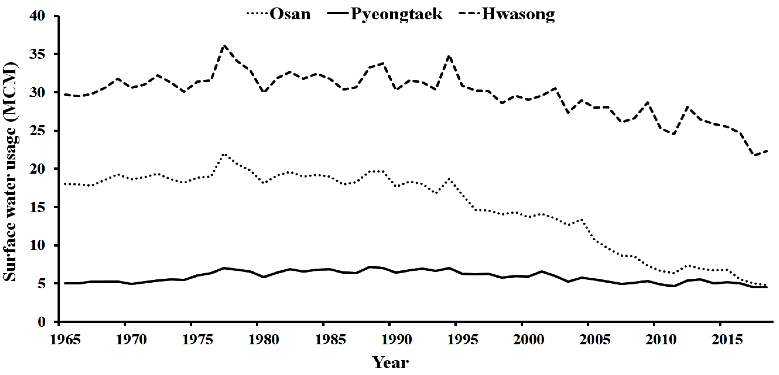
Figure 3.
Yearly groundwater usage in the Osan watershed.

Figure 4.
Average observed values for groundwater levels in the Osan watershed.

Figure 5.
Single-layer neutral network architecture.

Figure 6.
Process flow of the JA.

Figure 7.
Schematic representation of the linked S-O model.

Figure 8.
Observed and simulated groundwater values for the (a) Osan (b) Hwasong (c) Pyeongtaek subareas by using the ANN.
Figure 8.
Observed and simulated groundwater values for the (a) Osan (b) Hwasong (c) Pyeongtaek subareas by using the ANN.
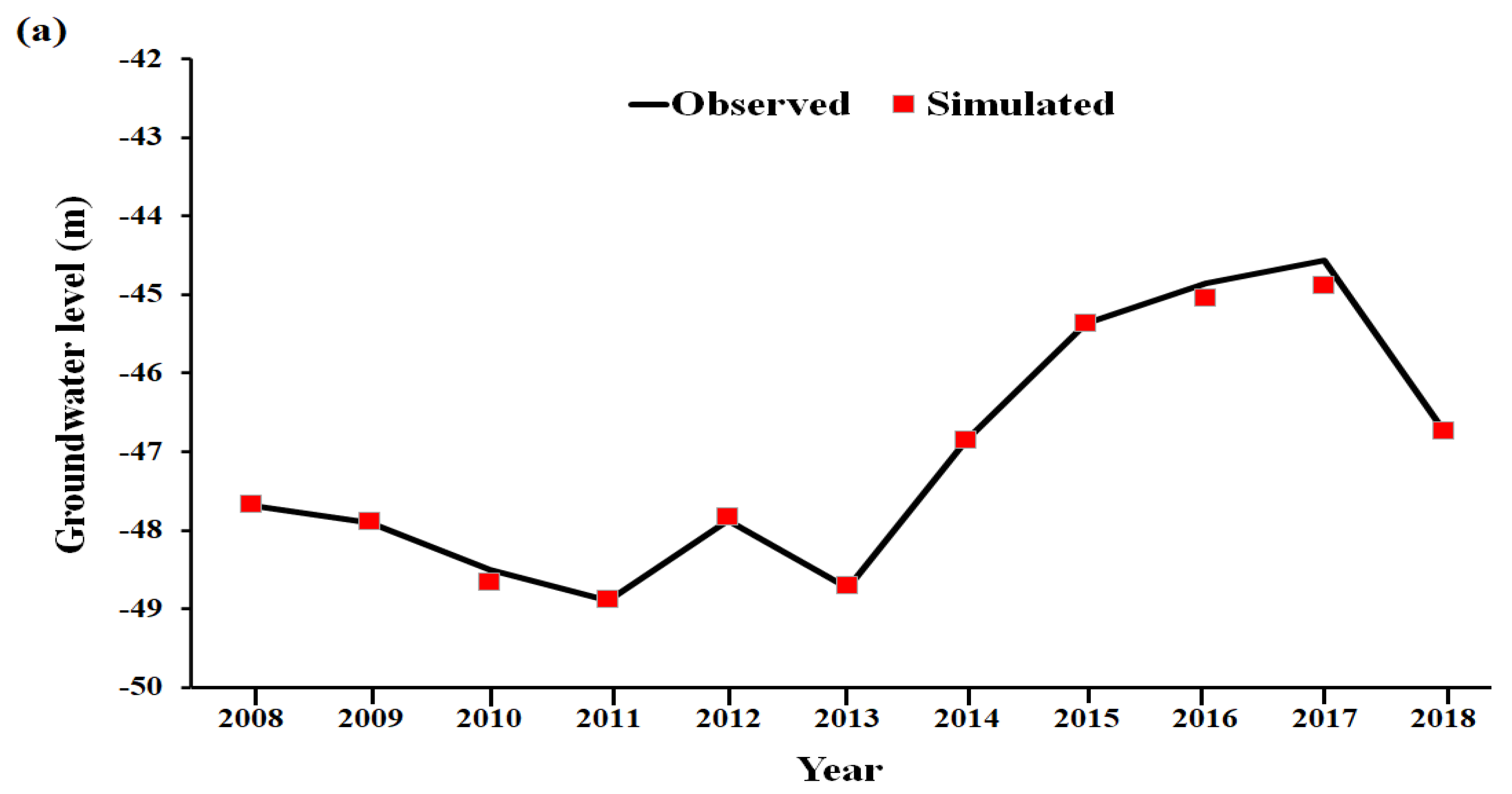

Figure 9.
Water demand, total water supply, and optimized water supply in the Osan watershed for the (a) Osan, (b) Hwasong and (c) Pyeongtaek subareas.
Figure 9.
Water demand, total water supply, and optimized water supply in the Osan watershed for the (a) Osan, (b) Hwasong and (c) Pyeongtaek subareas.


Figure 10.
Change in the groundwater level with and without conjunctive use in the Osan subarea.

Figure 11.
Convergence graph of the objective function.


Table 1.
Crop water requirement, water supply, and water demand in the Osan watershed.
| Year | Crop Water Requirement (mm) | Groundwater Supply (MCM) | Surface Water Supply (MCM) | Water Demand (MCM) |
|---|---|---|---|---|
| 2008 | 1833.4 | 0.34 | 24.78 | 44.18 |
| 2009 | 1909 | 1.20 | 25.52 | 46.01 |
| 2010 | 1986.1 | 1.12 | 22.79 | 47.87 |
| 2011 | 2118.6 | 1.18 | 22.14 | 51.06 |
| 2012 | 2031.8 | 1.21 | 25.33 | 48.97 |
| 2013 | 1686 | 1.20 | 24.12 | 40.63 |
| 2014 | 1653.3 | 1.27 | 23.41 | 39.84 |
| 2015 | 1545.5 | 1.32 | 23.42 | 37.25 |
| 2016 | 1602.6 | 1.60 | 22.04 | 38.62 |
| 2017 | 1858.5 | 1.51 | 19.62 | 44.79 |
| 2018 | 1679 | 1.30 | 19.51 | 40.46 |
Table 2.
Results of training and testing values for the ANN model.
| Subarea | Training (R) | Testing (R) | Overall (R) | Overall (R2) | RMSE | MSE | MAPE |
|---|---|---|---|---|---|---|---|
| Osan | 0.95 | 0.92 | 0.92 | 0.85 | 0.12 | 0.02 | 0.15 |
| Hwasong | 0.85 | 0.98 | 0.90 | 0.81 | 0.01 | 0 | 0.01 |
| Pyeongtaek | 0.99 | 0.97 | 0.99 | 0.98 | 0.02 | 0 | 0.08 |
Table 3.
Distribution of surface water, groundwater, total supply, and deficit with/without conjunctive use in the Osan watershed.
Table 3.
Distribution of surface water, groundwater, total supply, and deficit with/without conjunctive use in the Osan watershed.
| Subarea | Without Conjunctive Use (MCM) | With Conjunctive Use (MCM) | ||||||
|---|---|---|---|---|---|---|---|---|
| Surface Water Supply | Groundwater Supply | Total Water Supply | Deficit | Surface Water Supply | Groundwater Supply | Total Water Supply | Deficit | |
| Osan | 4.79–8.57 | 0.17–0.89 | 5.52–8.74 | 7.57–13.53 | 9.47–12.37 | 1.05–1.37 | 10.52–13.74 | 2.57–8.53 |
| Hwasong | 10.86–14.35 | 0.04–0.60 | 11.38–14.62 | 5.36–11.01 | 14.75–17.66 | 1.64–1.96 | 16.38–19.62 | 1.36–7.87 |
| Pyeongtaek | 2.26–2.75 | 0.02–0.13 | 2.30–2.88 | 1.03–2.65 | 2.97–3.49 | 0.33–0.39 | 3.30–3.88 | 0.03–1.65 |
Publisher’s Note: MDPI stays neutral with regard to jurisdictional claims in published maps and institutional affiliations. |
© 2021 by the authors. Licensee MDPI, Basel, Switzerland. This article is an open access article distributed under the terms and conditions of the Creative Commons Attribution (CC BY) license (https://creativecommons.org/licenses/by/4.0/).
Share and Cite
MDPI and ACS Style
Ashu, A.B.; Lee, S.-I. Simulation-Optimization Model for Conjunctive Management of Surface Water and Groundwater for Agricultural Use. Water 2021, 13, 3444. https://doi.org/10.3390/w13233444
AMA Style
Ashu AB, Lee S-I. Simulation-Optimization Model for Conjunctive Management of Surface Water and Groundwater for Agricultural Use. Water. 2021; 13(23):3444. https://doi.org/10.3390/w13233444
Chicago/Turabian StyleAshu, Agbortoko Bate, and Sang-Il Lee. 2021. "Simulation-Optimization Model for Conjunctive Management of Surface Water and Groundwater for Agricultural Use" Water 13, no. 23: 3444. https://doi.org/10.3390/w13233444
Note that from the first issue of 2016, this journal uses article numbers instead of page numbers. See further details here.