
A Novel Runoff Forecasting Model Based on the Decomposition-Integration-Prediction Framework
by
 , ,
, ,
Zhanxing Xu
1,2 ,
,
Jianzhong Zhou
1,2,*,
Li Mo
1,2,
Benjun Jia
1,2,
Yuqi Yang
1,2,
Wei Fang
1,2 and
Zhou Qin
1,2 1
School of Civil and Hydraulic Engineering, Huazhong University of Science and Technology, Wuhan 430074, China
2
Hubei Key Laboratory of Digital Valley Science and Technology, Wuhan 430074, China
*
Author to whom correspondence should be addressed.
Water 2021, 13(23), 3390; https://doi.org/10.3390/w13233390
Submission received: 10 November 2021
/
Revised: 20 November 2021
/
Accepted: 23 November 2021
/
Published: 1 December 2021
(This article belongs to the Section Hydrology)
Abstract
:Runoff forecasting is of great importance for flood mitigation and power generation plan preparation. To explore the better application of time-frequency decomposition technology in runoff forecasting and improve the prediction accuracy, this research has developed a framework of runoff forecasting named Decomposition-Integration-Prediction (DIP) using parallel-input neural network, and proposed a novel runoff forecasting model with Variational Mode Decomposition (VMD), Gated Recurrent Unit (GRU), and Stochastic Fractal Search (SFS) algorithm under this framework. In this model, the observed runoff series is first decomposed into several sub-series via the VMD method to extract different frequency information. Secondly, the parallel layers in the parallel-input neural network based on GRU are trained to receive the input samples of each subcomponent and integrate their output adaptively through the concatenation layers. Finally, the output of concatenation layers is treated as the final runoff forecasting result. In this process, the SFS algorithm was adopted to optimize the structure of the neural network. The prediction performance of the proposed model was evaluated using the historical monthly runoff data at Pingshan and Yichang hydrological stations in the Upper Yangtze River Basin of China, and seven various single and decomposition-based hybrid models were developed for comparison. The results show that the proposed model has obvious advantages in overall prediction performance, model training time, and multi-step-ahead prediction compared to several comparative methods, which is a reasonable and more efficient monthly runoff forecasting method based on time series decomposition and neural networks.
1. Introduction
Flood control and power generation are the two important operation objectives of reservoirs; accurate runoff forecasting provides reliable information of inflow in the forecast period so as to maximize the flood control benefits of the reservoir. It can also provide effective and exact input conditions for the preparation of power generation plans of hydropower stations to guide the economic and optimized operation of hydropower stations [1]. Therefore, accurate runoff forecasting is crucial. However, the formation process of hydrological runoff is affected by rainfall, evaporation, underlying surface conditions, and human activities. The runoff time series usually shows nonlinear and non-stationary characteristics [2,3,4,5]. In addition, many factors can impact the streamflow from upstream to downstream, such as tributaries, agricultural utilization, and dams; accurate runoff prediction is thus difficult and challenging [6,7,8].
In the past few decades, several runoff forecasting methods and models have been developed, ranging from conceptual models based on physical formation processes to fully data-driven models [9,10,11,12]. Although conceptual models can help people understand the process of runoff formation clearly, they need substantial hydrological, meteorological, underlying surface conditions, other parameters, and empirical knowledge. Therefore, there are many restrictive factors in the application of such models, resulting in poor prediction performance and uncertainty. For example, it is difficult to obtain good prediction results for some small basins lacking data [13,14]. In recent years, data-driven runoff prediction models have been widely studied and applied. Such models do not need to deeply understand the formation mechanism of the runoff process, but only need to predict runoff by fitting the nonlinear mapping relationship between input and output samples. Therefore, data-driven prediction models are becoming increasingly popular [1,15].
Data-driven forecasting models are also divided into two categories, namely the time series analysis model and the machine learning model [11]. Common time series analysis models include the Autoregressive model (AR), Moving Average model (MA), Autoregressive Moving Average model (ARMA), and Autoregressive Integrated Moving Average model (ARIMA) [16]. However, stationarity is a sufficient and necessary condition for establishing time series models, which makes these models difficult to capture the nonstationary of runoff time series [12]. In contrast, because of its strong nonlinear fitting ability and advantages of nonstationary series processing, the machine learning models are widely introduced into runoff forecasting research, from the Back Propagation (BP) neural network model, which was initially applied to runoff forecasting to Support Vector Machine (SVM) [1,17,18], Extreme Learning Machine (ELM) [8,19,20,21], and other machine learning models [22,23]. However, these classical models are easy to fall into local optimum and sensitive to parameter selection. Since the development of artificial intelligence, some deep learning methods, such as Recurrent Neural Network (RNN), have been tried to predict runoff because of its ability to learn long-term dependencies between runoff series [24]. Currently, the Long Short-Term Memory (LSTM) model is mostly studied [15,25], which can effectively overcome the shortcomings of gradient explosion and gradient disappearance in the general RNN model. Recently, Gated Recurrent Unit (GRU) [26], a variant of the LSTM network, has attracted researcher’s attention. Compared with LSTM, GRU has a simpler structure, fewer parameters, shorter training time, and has similar prediction performance with LSTM [27]. GRU has also been proved to have good application potential in runoff prediction [28].
Owing to the complexity of runoff series composition, the single runoff forecasting model is difficult to fully extract the internal components and identify the trend of runoff series, which affects the prediction performance [12]. Therefore, some researchers have begun to introduce signal time-frequency decomposition technology to preprocess original runoff series, fully extract useful information hidden in complex hydrological runoff series and construct a decomposition-based hybrid forecasting model to improve the overall prediction accuracy [16,29]. Discrete Wavelet Transform (DWT) is the most commonly used time-frequency analysis method in the hydrological field and has been widely used in runoff prediction [30,31]. However, the decomposition effect of DWT depends on the selection of the mother wavelet function and the setting of decomposition level, and its adaptability is poor [32]. Other wavelet analysis methods are more and more used in hydrology, such as Cross Wavelet Transform (XWT), and Wavelet Coherence Transform (WCT), which show good application results in the study of climate hydrological response [6,33]. Recently, some advanced wavelet time-frequency methods have been proposed, such as Least-Squares Wavelet Analysis (LSWA) and Least-Squares Cross Wavelet Analysis (LSCWA) [7]. These methods do not need any interpolation, gap-filling, or de-spiking, and have outstanding advantages in analyzing hydrological time series. LSCWA can be used to analyze the influence relationship between the two sequences and estimate the trend and seasonal components of hydrological time series more accurately, it can effectively reveal the possible consistency of climate and runoff time series components. In addition, EMD is also the most commonly used time-frequency decomposition method in some research [34,35]. This method can adaptively decompose the original time series into multimodal functions according to the characteristics of the original time series, which makes up for the deficiency of DWT to a certain extent, but there is a problem of modal aliasing, which is easy to cause the in-complete separation of noise series [36]. Variational Modal Decomposition (VMD) is an emerging signal time-frequency decomposition method [37]. It decomposes the original sequence into a set of modal functions with limited bandwidth by solving the variational problem. It has better anti-noise ability and mathematical theory foundation than classical DWT and EMD. It has been successfully applied to the prediction of different time series [38,39,40,41]. In recent years, it has also been gradually introduced into the analysis and prediction of runoff series [1,20].
At present, most of the decomposition-based hybrid runoff forecasting models with time series decomposition are based on the framework of Decomposition-Prediction-Reconstruction (DPR). Under this framework, the runoff forecasting results are obtained by predicting the sub-series decomposed from the original runoff series respectively and then aggregating the predicted values of the sub-series [1,12,20,42]. The research of hybrid runoff forecasting models mainly focuses on combining different time-frequency decomposition techniques and different machine learning methods, improving the prediction accuracy of the model by selecting improved decomposition techniques and some new machine learning models [9,12,43]. The prediction accuracy of the models can be improved effectively in some models, but many works are similar. At the same time, in this framework, the runoff decomposition level number determines the number of sub-prediction models, which in turn require more training time for such hybrid models [44]. On the other hand, the DPR framework obtains the final runoff forecasting result by overlaying the prediction results of each sub-series, which is easy to cause the accumulation of prediction error of each sub-series and make the runoff forecasting result deviate greatly, especially in the peak part of runoff series. Moreover, due to the complexity of the structure of deep learning models, such as LSTM and GRU, the inappropriate network structure will cause the loss of prediction accuracy and training time. Therefore, it is necessary to adopt the appropriate hyper-parameter optimization method with better global search ability to select the best structure parameter configuration for neural network models [45].
In summary, to explore the better hybrid application model of time-frequency decomposition technology and machine learning method for runoff forecasting, we developed a novel runoff forecasting framework and proposed a runoff forecasting model under this framework. The contributions of this research include:
- (1)
- The development of a runoff forecasting framework named Decomposition-Integration-Prediction (DIP) using parallel-input neural network, and proposed a novel runoff forecasting model with VMD, GRU, and Stochastic Fractal Search (SFS) algorithm under this framework;
- (2)
- The application the model to the runoff forecasting of Pingshan and Yichang Hydrological Stations in Upper Yangtze River Basin, China, and then verified the reliability and prediction performance of this forecasting method;
- (3)
- We further highlight the rationality and advantages of the proposed hybrid forecasting model by employing the seven models as comparative forecast models in terms of combinatorial principle and evaluating indicator, including AR, BP, LSTM, GRU, and three decomposition-based hybrid models Variational Mode Decomposition-Long Short-Term Memory (VMD-LSTM), Variational Mode Decomposition-Gated Recurrent Unit (VMD-GRU), Variational Mode Decomposition-Gated Recurrent Unit-Stochastic Fractal Search (VMD-GRU-SFS) based on the DPR framework.
The remainder of this paper is organized as follows: Section 2 briefly introduces the above-mentioned methods and presents the details of the proposed framework for monthly runoff forecasting. Section 3 contains several prediction performance evaluation indicators selected. Section 4 presents the case studies of the monthly runoff forecasting for the proposed method and contrast methods. Section 5 carries out result analysis and discussion, and the conclusions are provided in Section 6. Abbreviation descriptions of this paper are shown in Table A1.
2. Methodologies
2.1. Variational Mode Decomposition
To address the limitations of EMD for sensitivity to noise and sampling, Variational Mode Decomposition (VMD), an adaptive nonstationary signal decomposition method, was proposed by Dragomiretskiy and Zosso [37]. EMD uses recursive decomposition to extract sub-signals with different frequencies [46]. In contrast, the significant difference is that VMD uses the non-recursive method to transform the signal decomposition into a constrained variational problem. Its goal is to minimize the sum of the estimated bandwidth of each mode and uses the Alternate Direction Method of Multipliers (ADMM) algorithm to continuously update each mode and its center frequency, and gradually shift the mode’s frequency spectrum to “baseband”. Finally, each mode and its center frequency are extracted together. In this process, we need to assume that each mode is a finite bandwidth with different center frequencies. The constrained variational problem can be expressed as follows:
where is the kth mode, is the center frequency of the kth mode, is the Dirac distribution, × denotes convolution, and is the given observed signal.
In order to render the problem unconstrained. The quadratic penalty factor and Lagrangian multiplier are introduced to transform the constrained variational problem into an unconstrained problem of the following equation:
where and are the penalty parameter and Lagrange multiplier, respectively. Parameter can effectively reduce the interference of Gaussian noise, and can enhance the strictness of the constraint.
Therefore, the original minimization problem is now converted to an alternative model, in which, ADMM is adopted to seek the saddle point of the Lagrangian function by alternately updating the mode , frequency , and Lagrangian multiplier . The iterative equations of , , , are as follows:
where is the number of iterations, , , , and denotes the Fourier transforms of , , , and , respectively.
2.2. Gated Recurrent Unit
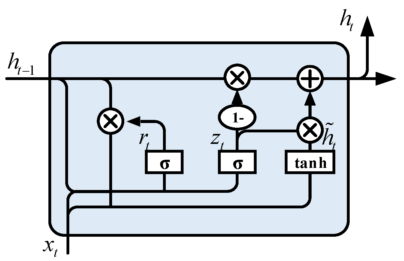
Gated Recurrent Unit (GRU) [26,27] is a neural network model first proposed by Cho et al. in 2014 to capture the long-term dependence of time series. GRU network can be regarded as a very effective variant of the LSTM network. Its structure is simpler than the LSTM network and it requires less time for model training [28]. Therefore, the GRU model has been widely used in the field of artificial intelligence [27,47], especially in processing time series [48,49]. LSTM import three gate operations: input gate, forgetting gate, and output gate to control input value, storage value, and output value [50]. In the GRU model, gate operations are simplified to update gate and reset gate. The specific structure of GRU is shown in the following Figure 1:
GRU cell is mainly composed of update gate and reset gate . The update gate controls the degree to which the state information at the previous time step will be brought into the current time step. The larger the value of the update gate is, the more the state information at the previous time step is brought in; reset gate is used to control how much information from the previous state is written into the current candidate set. More historical information will be ignored when the reset gate approaches the biggest value 1. The calculation equation between variables is as follows:
where, subscript denotes the current time step, , , represents the weights matrixes of the reset gate, the update gate, the hidden state in the GRU cell, respectively. Parameters
,
, and denotes the different biases corresponding to the different weight matrices. Parameter
is the calculated element of the hidden state (), and the symbol is an element-wise multiplication.
2.3. Stochastic Fractal Search Optimization
Stochastic Fractal Search algorithm (SFS) searches the optimal solution by the diffusion property of fractal [51,52,53]. The algorithm mainly includes two processes: diffusion process and update process. In diffusion process, the Gaussian distribution is selected as the random walk mode, in which each individual is diffused around its current position to generate a new generation. This step can be regarded as the exploitation phase of SFS algorithm. For each individual that diffuses, the position of each new individual is created through Gaussian walking and find the best individual among all individuals. The Gaussian walking function can be expressed as one of the following two equations:
where and are random numbers between [0, 1], is the optimal individual, is the position of the ith particle, and are Gaussian distribution parameters.
After, the update process is carried out, which can be considered as the exploration stage of the SFS algorithm. The process consists of two updates. The first update is for individual components, and the chance of individual component change is determined by sorting individual fitness values and calculating performance indicators. The better the individual fitness, the greater the chance of individual component change. The change equation of performance index and individual component is as follows:
where is the new modified position of , and are random selected individuals in the population.
The second update process aims to change the position of an individual by considering the position of other individuals in the population. This procedure improves the quality of exploration and thus meets the attributes of diversity. Before the second update process begins, all individuals obtained from the first update process need to be sorted again based on Equation (10), and then modify the position of as follows:
where is the position of the individual after the second update, and are two different random points selected from the group, is the best point and is a random number within the range [0, 1].
2.4. The Novel Runoff Forecasting Model Based on DIP Framework
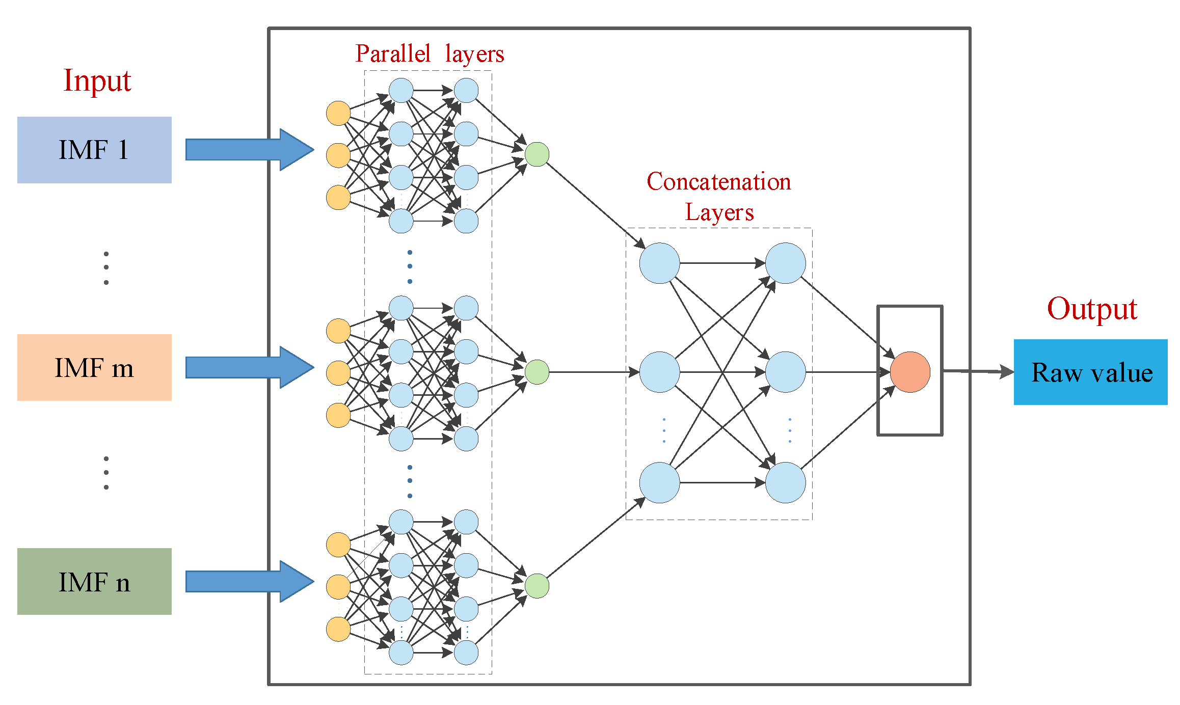
As a result of climate change and human activities, hydrological time series are often nonlinear and nonstationary [2,54]. To explore the better application of time series decomposition technology in runoff forecasting and enhance the prediction accuracy effectively, we developed a framework of runoff forecasting named Decomposition-Integration-Prediction (DIP) using a parallel-input neural network, and proposed a novel runoff forecasting model using VMD-GRU-SFS (DIP) with VMD, GRU, and SFS algorithms under this framework, as shown in the Figure 2, the parallel-input neural network structure illustrated in Figure 3.
In the developed DIP framework, the observed runoff series is first decomposed into several sub-series via the time series decomposition method to extract different frequency information and reduce the difficulty of the model prediction. Secondly, the parallel layers in the parallel-input neural network are trained to receive the input samples of each subcomponent and integrate their output adaptively through the concatenation layers. Finally, the output of concatenation layers is treated as the final runoff forecasting result. In this process, the hyper-parameter optimization algorithm is used to optimize the structure of the neural network to obtain the best prediction performance. Under the DIP framework, VMD, GRU, and SFS are adopted to form a model of a novel runoff forecasting hybrid model VMD-GRU-SFS (DIP), in which VMD is used to decompose the original runoff series, GRU is selected to establish the parallel-input neural network, SFS is adopted to optimize hyper-parameter of the model. Meanwhile, it is important to note that when we train the model, the output samples of the model are the raw observed series, not the sub-series of decomposition.
The structure of the constructed parallel-input neural network mainly includes two composite layers. The first layers are the parallel layers, in which several parallel neural networks are used to receive the input variable samples of each runoff sub-components. The second layers are the concatenation layers, the output of each parallel neural network is adaptively aggregated through the concatenation layer network to output the predicted runoff value.
The overall procedure used by the proposed forecasting method can be described as the following steps.
- (1)
- Data Pre-processing. Data cleaning is first used to process the runoff time series if the consistency check result is rejected. Next, we use VMD to decompose the runoff data into a set of sub-series with different frequencies. For optimal selection of decomposition level, check whether the last extracted component exhibits central-frequency aliasing. Then, the data in all sub-series are divided into training and testing datasets that are normalized to a range of [0, 1] aswhere and are the normalized and raw value of the ith runoff data sample, respectively. Parameters and are the maximum and minimum of data samples.
- (2)
- Lag period selection. For each sub-series decomposition by VMD, Partial Autocorrelation Function (PACF), is used to select the optimal Lag period for generating modeling samples, where the PACF lag count is set to 36. Assuming is the value to be predicted of the kth runoff component, we select the values which PACF exceeds 95% confidence interval in the 36 delay periods of time t as the input variables for this sub-series.
- (3)
- Model training & Hyper-parameters optimization. Using some open-source software libraries, such as Tensorflow and Keras, to build and training the multi-input neural network. To improve the forecasting performance, SFS is applied to optimize the hyper-parameters of the proposed framework. In this work, we mainly consider the numbers of hidden layers and hidden nodes for parallel layers and concatenation layers in parallel-input neural network. The number of hidden layers is initialized from 1 to 3 and the number of hidden nodes ranging from 5 to 100.
- (4)
- Forecasting application. In the third step, the parallel-input neural network has been trained. In forecasting application, the prediction result of the model should be denormalized to obtain the final predicted value.
3. Model Evaluation
In this section, four statistical indicators are employed for evaluating the forecasting performance of the proposed framework, namely Root Mean Square Error (RMSE), Normalized Root Mean Square Error (NRMSE), Mean Absolute Percentage Error (MAPE), and Nash-Sutcliffe Efficiency coefficient (NSE). RMSE and NRMSE can effectively describe the loss of regression; MAPE is used to test the relative error between the predicted value and the observed value; NSE is adopted to measure the consistency between the runoff forecast process and the actual process, and can evaluate the stability of the prediction results. Generally, forecast models with larger values of NSE or smaller values of RMSE, NRMSE, and MAPE provide better forecasting performance. These four performance metrics are defined as follows:
4. Case Studies
4.1. Study Area and Dataset
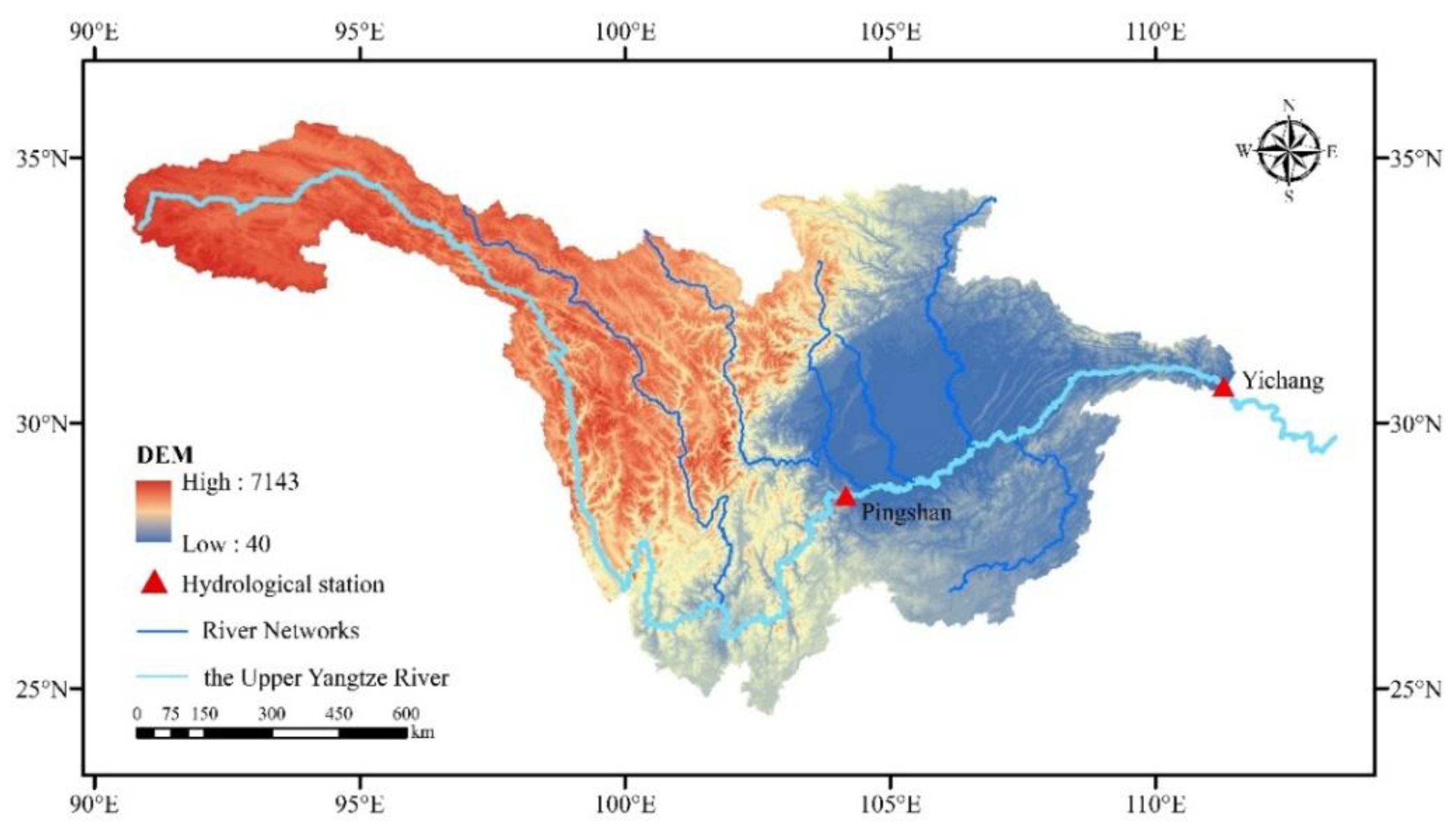
In this research, the Upper Yangtze River (UYR) Basin, from the source of the Yangtze River to Yichang, Hubei Province, is considered as the study object. As shown in Figure 4, the basin area is about of 1 × 10⁶ km2 (90°55′–111°52′ E, 24°49′–35°71′ E), approximately 55% of the total area of the Yangtze River Basin [55]. The UYR includes nine provinces, autonomous regions, and municipalities, including Qinghai, Tibet, Sichuan, Yunnan, Chongqing, and Hubei. The topography of the basin is complex and diverse, including the plateau (Qinghai Tibet Plateau) and the basin (Sichuan Basin), with an altitude level ranging from about 40 to 7143 m above sea level. Influenced by the southeast monsoon, southwest monsoon and Qinghai Tibet Plateau, the climate in this area is very sensitive and the rainfall distribution is significantly uneven. The flood season usually occurs from May to September, which accounts for 78% of the total annual rainfall, while the dry season is affected by water shortage. Therefore, the impact of climate diversity has brought many difficulties to the development and utilization of water resources in the region [43].
The monthly runoff data analyzed in this paper are from the Pingshan and Yichang hydrological station in UYR Basin, two key control stations in Upper Yangtze River. Their position is shown in Figure 4. The monthly runoff data covers the period from January 1940 to December 2010 for Pingshan, and January 1884 to December 2020 for Yichang, respectively. 80% of the monthly runoff data were used for training, 20% were used for testing. In the training dataset, approximately 90% of the data were utilized for model parameter optimization and the remainder were utilized for validation. In this work, all of the data preprocessing and management was performed by Numpy and Pandas scientific computing package in Python.
4.2. Data Preparation
To reduce the difficulty of prediction, VMD was utilized to decompose the original runoff series. The setting of decomposition parameter K is crucial to the decomposition result; too large or too small will affect the prediction accuracy directly. In our work, through the iterative calculation of K from 2 to 20, when K = 9, there was mode aliasing, so we could determine the optimal number of decomposition levels K = 8 [56]. The frequencies of the generated subseries varied from low to high, which indicates the components of the runoff series are quite complicated. After decomposition, the complexity level of the forecast greatly decreased due to the more regular data pattern.
Generally, the selection of input variables of the prediction model is of significance in the performance of predictions, so it is necessary to optimize the selection of input variables. Previous research has established that sequence decomposition may reduce the correlation between subcomponents and meteorological factors [57]. Therefore, in this study, we only used historical data autocorrelation to predict runoff. According to the procedure of Section 2.4, PACF is used to determine the optimal lag period. After calculation, the PACF of each subsequence was different. On the basis of fully considering the information in PACF and domain knowledge in practical application, the input variables for each series of the Yichang station monthly runoff forecasting model are listed in Table 1, where Xt-n denotes the nth antecedent variables of the sample to be predicted. The different number of input variables for each sub-series prediction model also explains the complexity of runoff sequence composition and the difficulty of forecasting.
4.3. Model Parameter
After data preparation of monthly runoff series for two hydrological stations, a proper forecasting model was selected, which can be used for runoff series. According to Section 2.4, we built a VMD-GRU-SFS (DIP) runoff forecasting model based on the DIP framework. The model parameters of VMD-GRU-SFS (DIP) for Pingshan and Yichang stations were optimized by the SFS algorithm, including the number of hidden layers and node number of hidden layers of each parallel GRU neural network, the hidden layers, and the number of node number of hidden layers of concatenation layers. The optimized network parameters are summarized in Table 2, where Adam, an extension to stochastic gradient descent, is selected as the optimizer [58].
4.4. Comparative Experiment Develop
To verify the rationality and prediction accuracy of the proposed runoff forecasting method, seven forecasting models were developed for comparison: four single forecasting models of AR, BP, LSTM, and GRU and three decomposition-based hybrid models of VMD-LSTM, VMD-GRU, and VMD-GRU-SFS. These models were implemented in Python programming. For the standard BP, LSTM, and GRU neural network models, the prediction problem can be directly transformed into a supervised learning problem, in which the observed runoff series of length N were divided into N−L data samples (where L is the length of the lag period), the input of the model is the L observation data before the forecast value, and the output is the forecast target. In general, the three-layer structure is proven to be able to fit arbitrary nonlinear functions [41]. Therefore, a three-layer structure was selected for these models. By contrast, for the hybrid forecasting method VMD-LSTM and VMD-GRU, the original runoff was first divided into several sub-series utilizing VMD. Each sub-components were then modeled utilizing a standard LSTM or GRU, respectively, and finally aggregated results of individual sub-series to obtain the final forecasting results. In addition, VMD-GRU-SFS combined with the SFS method to optimize the parameters of the model based on VMD-GRU, which is helpful in the selection of a more suitable model structural hyper-parameters. It should be noted that the above three hybrid models are based on the DPR prediction framework.
5. Result Analysis and Discussion
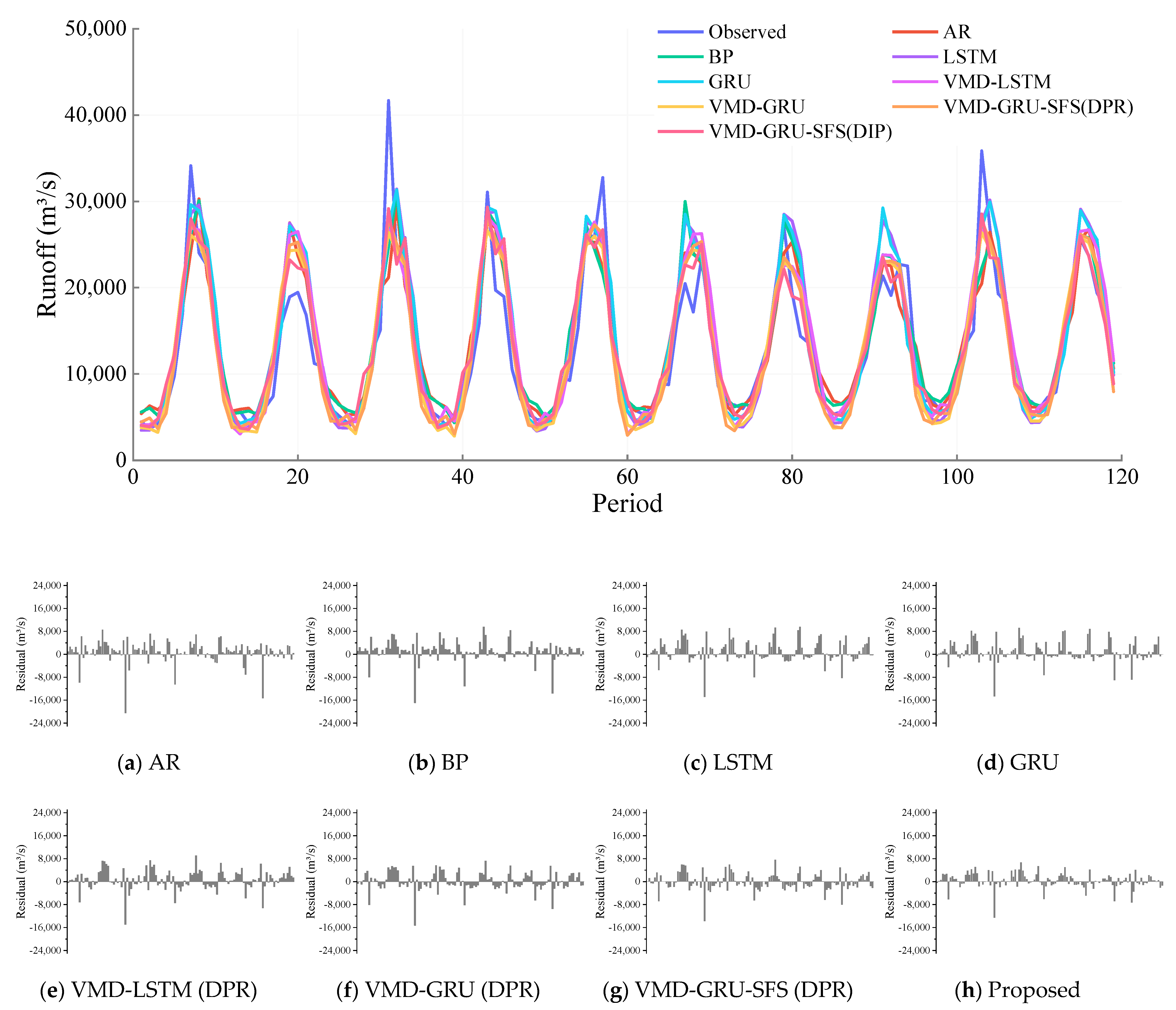
Based on the descriptions above, the forecast results of the proposed method and the contrast methods including AR, BP, LSTM, GRU, VMD-LSTM (DPR), VMD-GRU (DPR), and VMD-GRU-SFS (DPR) are discussed in this section. Figure 5 and Figure 6 show the comparison chart of prediction process and residual process of eight different prediction models in testing period for the Pingshan and Yichang stations. Figure 7 and Figure 8 show the scatter plot of the runoff series prediction results in testing period for the Pingshan and Yichang stations. In general, the prediction accuracy of the hybrid runoff forecasting model based on time series decomposition is higher than that of the single prediction model, and after SFS hyper-parameters optimization, the prediction accuracy of model has been effectively improved.
It can be seen from Figure 5 and Figure 6 that the prediction results of various models are essentially in line with the fluctuation process of runoff series in Pingshan and Yichang stations, and the prediction accuracy is ranked from high to low as: proposed model > VMD-GRU-SFS (DPR) > VMD-GRU (DPR) > VMD-LSTM (DPR) >GRU > LSTM > BP > AR. In the single prediction model, the AR and BP models have poor fitting ability and high prediction error. Compared with AR and BP, the LSTM model has recurrent neural network structure, which can better learn the long-term dependence of runoff series, the prediction accuracy of the model is improved. GRU model is a variant of LSTM, which simplifies the model structure without losing the prediction accuracy, and the prediction accuracy is basically consistent with LSTM. By contrast, the prediction performance of hybrid model is always better than single model, which can better fit the peak flow and have better prediction accuracy. However, the neural network model parameters are more difficult to select, which may lead to under-fitting and over-fitting. By using the SFS optimization algorithm to optimize the parameters of the GRU model, the prediction performance of the model can be obviously improved. Moreover, it is apparent from these figures that the prediction results of the proposed VMD-GRU-SFS (DIP) method based on DIP framework are always better than the other seven comparison models.
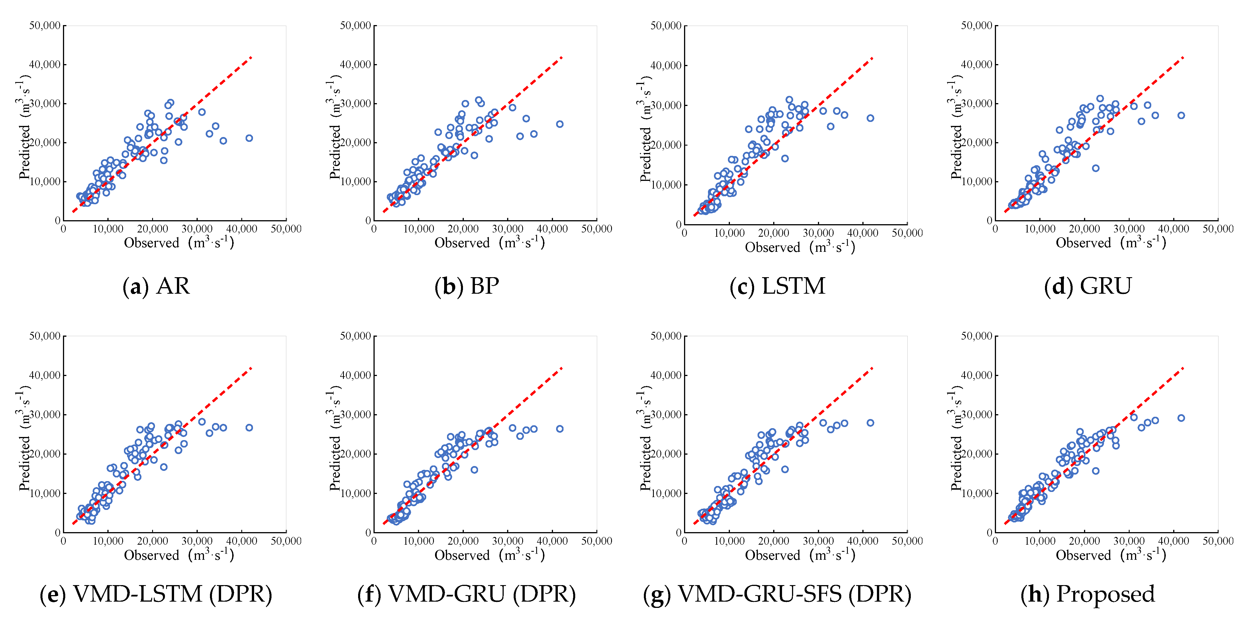
It can be clearly seen from the scatter diagram of Figure 7 and Figure 8 that the prediction performance of various models is obviously different. The scattered points of AR and BP models deviate far from the ideal line, especially the peak part of runoff. The prediction effects of LSTM and GRU models are similar, which are improved compared with above two models on the whole, but the scatter points are still relatively scattered. In general, it is obvious through the scatter plot that the prediction performance of the decomposition -based hybrid model is significantly better than that of the single model. However, at the peak of runoff, the scatter points of the VMD-LSTM (DPR) and VMD-GRU (DPR) model deviated from the ideal fitting line. By comparison, the VMD-GRU-SFS (DPR) model optimized with hyper-parameters has less deviation at the peak. The most striking finding is that for two hydrological stations, the forecasted and observed data scatter points of the proposed model are very close to the ideal baseline, whether it is the whole or the peak prediction part, which shows that the proposed method can effectively improve the generalization ability of the runoff forecasting model.
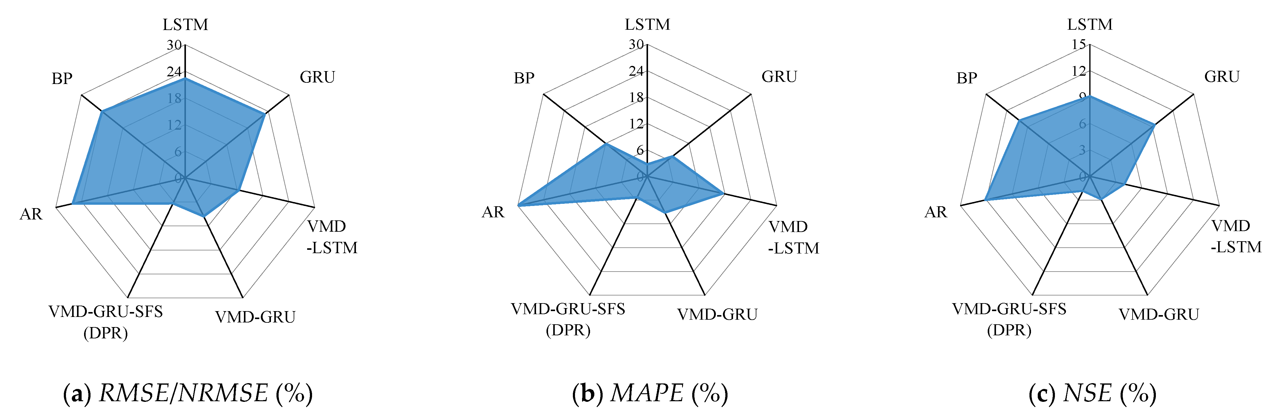
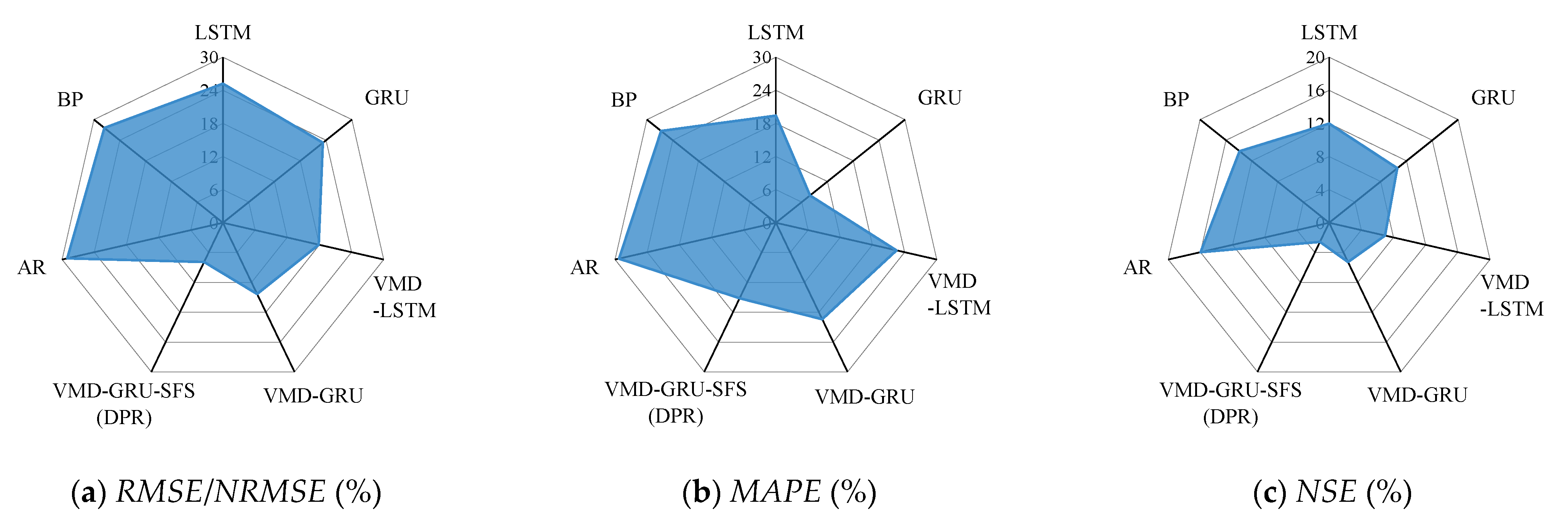
Although the predicted-observed runoff comparison hydrograph and scatter diagram can intuitively evaluate the corresponding relationship between the predicted value and the observed data, the statistical indicators can more accurately evaluate the prediction ability of a different model. To decrease the accidental error of neural network model, the statistical indexes were obtained after 10 trainings and the average value was calculated. Table 3 and Table 4 show the evaluation results of eight models in Pingshan and Yichang stations during training period and testing period. Figure 9 and Figure 10 show the prediction performance improvement ratio of the proposed model compared with other models for two stations.
In summary, the application of time series decomposition algorithm and hyper-parameter optimization method can enhance the prediction performance of the runoff forecasting model. Compared with GRU and VMD-GRU (DPR), the NSE of VMD-GRU-SFS (DPR) model in the testing set of both Pingshan and Yichang stations can be increased by more than 7% and 1%. It shows that time series decomposition can effectively reduce the difficulty of prediction by extracting the internal variation characteristics of runoff series, and also demonstrating the importance of hyper-parameter optimization to improve the accuracy of the forecasting model. Furthermore, one can clearly see from the table that the statistical indexes of the proposed runoff forecasting method are optimal in both the training period and the testing period. Taking Yichang station as an example, the RMSE, NRMSE, MAPE, and NSE in the test period are 3145.08, 8.28, 16.2, and 0.878, respectively. As shown in the Figure 10, the predicted statistical indexes during the test period of the proposed model have been improved to varying degrees compared with the other seven models. Compared with the single GRU model, the RMSE and NRMSE decreased by 23.3%, the MAPE decreased by 7.95% and the NSE increased by 10.6%. Compared with the VMD-GRU-SFS (DPR) hybrid model, RMSE and NRMSE decreased by 7.88%, MAPE decreased by 15.2%, and NSE increased by 2.57%. The analysis shows that the proposed runoff forecasting method can provide more satisfactory prediction results for runoff forecasting than other methods, and also demonstrates that the DIP prediction framework developed in this paper has better prediction performance than DPR framework for complex hydrological time series.
In addition, one interesting finding is that the training time of our proposed model is significantly less than that of other VMD-LSTM, VMD-GRU, and VMD-GRU-SFS hybrid models based on the DPR framework. Figure 11 shows the training time of different runoff forecasting models for the two stations. In general, the training time of a single model is much less than that of the hybrid model because of its simpler model structure and only requires training one runoff series. It should be pointed out that for the method with hyper-parameter optimization, the time for hyper-parameter optimization is not included, because the process of hyper-parameter optimization is very time-consuming.
Here we focus on the comparison of training time between hybrid models. As shown in the Figure 11, the training time of VMD-LSTM (DPR), VMD-GRU (DPR), VMD-GRU-SFS (DPR), and the proposed method in Pingshan station and Yichang station is shortened in turn. The VMD-LSTM (DPR) model in Pingshan station and Yichang station has 108 and 182.5 s training time respectively, and the total training time is the longest. Compared with VMD-LSTM (DPR), training time of the VMD-GRU (DPR) model is reduced because of its more concise structure, this finding is consistent with that of Gao et al. [28]. VMD-GRU-SFS (DPR) combines SFS hyper-parameter optimization based on VMD-GRU (DPR), it is helpful to find the best and most concise model structure, and the training time of the model is also significantly shortened. It is worth noting that the training time of the proposed model is the least in the hybrid model. The training time in the two stations is 64.9 s and 98.3 s, respectively, which is significantly reduced compared to the other three hybrid models. Taking Yichang station as an example, the training time of the proposed model is reduced by 46%, 42%, and 37% respectively compared with VMD-LSTM (DPR), VMD-GRU (DPR) and VMD-GRU-SFS (DPR). Therefore, the proposed method can save substantial model training time and has better practicability, which again proves the advantages of the method in runoff forecasting.
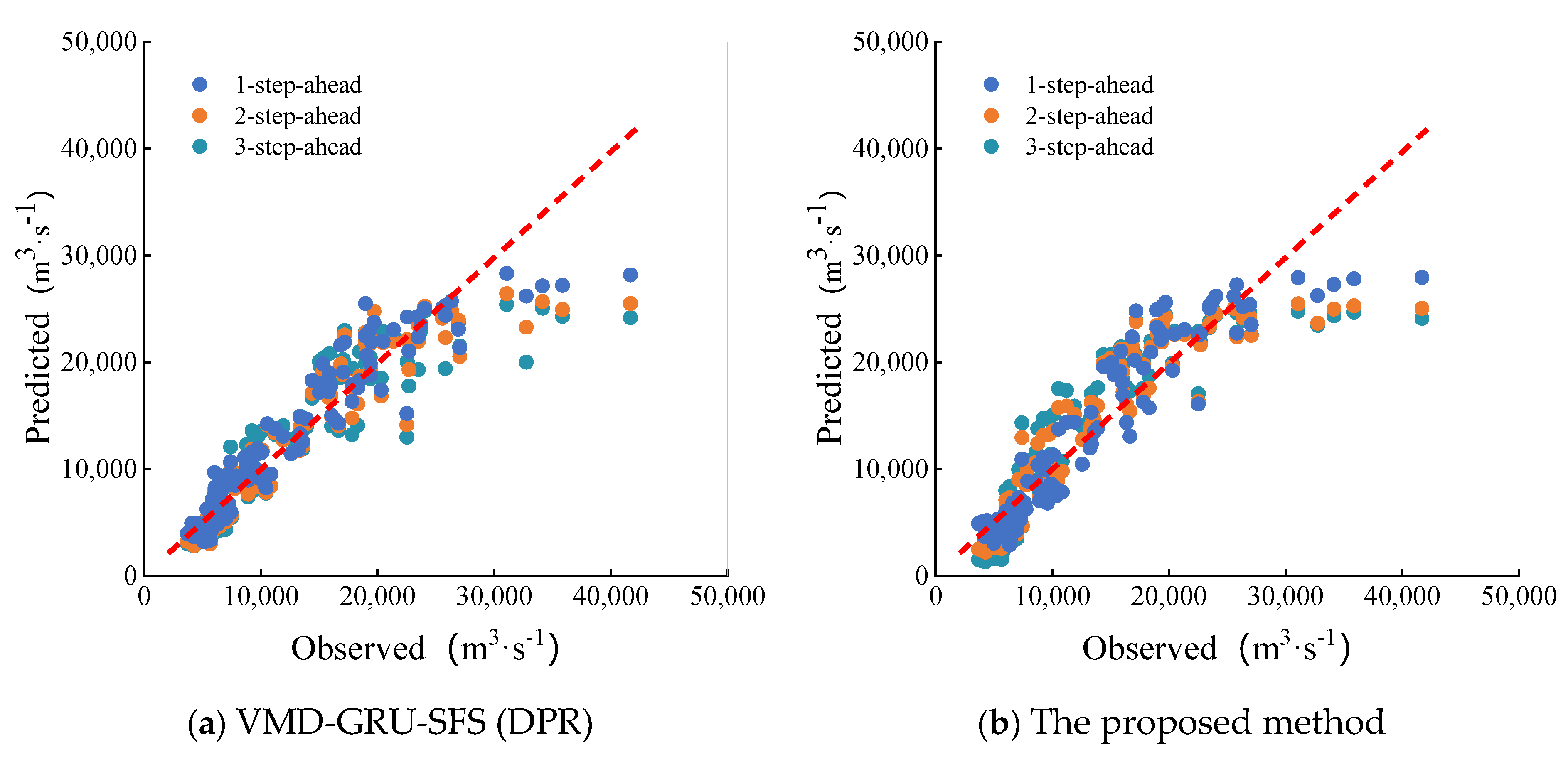
The studies above show that the performance of AR, BP, LSTM, GRU, VMD-LSTM (DPR), VMD-GRU (DPR), VMD-GRU-SFS (DPR), and the proposed model in single-step-ahead monthly runoff forecasting is different. The NSE of the proposed VMD-GRU-SFS (DIP) method of the testing set can reach 0.87 both in Pingshan and Yichang station, and both RMSE and MAPE are small. Compared with other models, the performance of the proposed model is improved to varying degrees, which shows a satisfactory monthly runoff forecasting ability. In addition to the accuracy of one-step prediction, multi-step monthly runoff forecasting is also of great significance for flood control and disaster reduction of reservoirs and compilation of long-term operation plans. Therefore, we can move on to discuss the multi-step-ahead forecasting performance of the proposed method next. The proposed method and VMD-GRU-SFS (DPR) model can be used as an example to compare the prediction results of the two models when the prediction steps are 1, 2 and 3. The scatter diagrams of the predicted and observed values of the two models with different prediction steps ahead are shown in Figure 12. Table 5 shows forecast results for the above two models for under the prediction steps of 1, 2 and 3.
It can be seen from the above figure that, on the whole, the prediction performance of the proposed method is better than the VMD-GRU-SFS (DPR) model for different prediction steps of 1, 2 and 3, and the scatter is relatively more concentrated. Especially in the peak part, the scatter of the proposed method is closer to the baseline when the flow exceeds 30,000 m3. With the increase of the prediction step size, the scattered points become more dispersed, and the prediction accuracy of the model decreases gradually. It seems that these results are due to the accumulation of prediction errors with the increase of prediction steps. It can be seen from Table 5 that with the increase of prediction steps, RMSE, NRMSE, and MAPE of VMD-GRU-SFS (DPR) model and the proposed model gradually increase, and the NSE value also decreases. When the three-step-ahead prediction is carried out, the NSE of VMD-GRU-SFS (DPR) model is 0.765, while NSE of the proposed model can still reach more than 0.8, indicating the better performance of the proposed model in multi-step prediction, it further shows the outstanding advantages of the proposed model in forecasting stability and extending the forecast period.
Via the above comparative analysis, the prediction results of the proposed VMD-GRU-SFS (DIP) method based on DIP framework are always better than the other seven comparison models in overall prediction performance, model training time, and multi-step-ahead prediction, mainly reasons for the superiority of the hybrid method are analyzed below. On the one hand, the parallel-input neural network in the proposed method adaptively aggregates the output of each parallel GRU model to obtain the prediction result. The model structure has the function of error self-calibration, which can effectively avoid the error accumulation in the integration of subsequence prediction results, thus achieving better single-step and multi-step prediction performance compared with other models. On the other hand, the parallel-input neural network obtains the decomposed runoff sub-series samples as the input and the original runoff sequence samples as the output. Although the structure of the model is more complex than that of single input, it only needs one model training, and does not need to train each sub-series separately. Therefore, it can save the training time of prediction model to a great extent.
6. Conclusions
In this paper, to improve the prediction performance of nonlinear, nonstationary runoff series, we proposed a novel runoff forecasting method based on the Decomposition-Integration-Prediction (DIP) framework. This method first involved obtaining the sub-series samples decomposed from the original runoff series by VMD as the model input. Then, several parallel GRU of the parallel-input neural network were used to fit trend, cycle, and seasonal variation characteristics of runoff subcomponents and integrate their output adaptively through the concatenation layers. Finally, the output of concatenation layers was treated as the final runoff forecasting result. In this process, we used the SFS algorithm to optimize the hyper-parameters of the model. In addition, using RMSE, NRMSE, MAPE, and NSE as the performance evaluation indices, the prediction results of the proposed method were compared with those of seven prediction models: AR, BP, LSTM, GRU, VMD-LSTM (DPR), VMD-GRU (DPR), and VMD-GRU-SFS (DPR).
In general, the method proposed in this paper can significantly improve the prediction performance of monthly runoff. Compared with the other seven runoff forecasting models, the key features of the proposed method lie in the following aspects:
- (1)
- This method can more effectively identify the internal variation characteristics of runoff series, adaptively aggregate the prediction results of sub-series, and improve the overall prediction accuracy of the model.
- (2)
- Compared with other hybrid runoff forecasting models based on DPR framework, this method can significantly shorten the training time of the model and has better practical value.
- (3)
- Compared with the VMD-GRU-SFS hybrid model based on DPR, the proposed method has better multi-step prediction ability and can effectively extend the prediction period.
The prediction results show that among all methods mentioned, the proposed method in this paper is the best on prediction accuracy, model training time, and multi-step-ahead prediction. Overall, the proposed new framework is a useful tool for forecasting nonlinear and nonstationary runoff series and is thus a promising model for runoff forecasting. However, it is worth noting that the main limitation of this study is that only the data series of two stations are used for model verification. Future research needs to be extended to stations in other basins to verify the robustness of the model. In addition, the proposed model needs interpolation pretreatment for the missing values in the runoff series. In the future, we will use advanced time-frequency analysis methods such as LSWA for runoff prediction research.
Author Contributions
Conceptualization, Z.X., J.Z. and L.M.; methodology, Z.X. and J.Z.; validation, Z.X., B.J. and Y.Y.; formal analysis, L.M.; data curation, W.F. and Z.Q.; writing—original draft preparation, Z.X.; writing—review and editing, L.M. and J.Z.; visualization, Z.X., B.J. and Y.Y.; supervision, J.Z. and L.M. All authors have read and agreed to the published version of the manuscript.
Funding
This paper is supported by the Key Program of the National Natural Science Foundation of China, grant number U1865202,52039004.
Institutional Review Board Statement
Not applicable.
Informed Consent Statement
Not applicable.
Data Availability Statement
Some data used during the study are proprietary or confidential in nature and may only be provided with restrictions.
Conflicts of Interest
The authors declare that they have no known competing financial interest or personal relationship that could have appeared to influence the work reported in this paper.
Appendix A

Table A1.
Abbreviation descriptions.
| Acronym | Full Name |
|---|---|
| DIP | Decomposition-IntegrationPrediction |
| VMD | Variational Mode Decomposition |
| GRU | Gated Recurrent Unit |
| SFS | Stochastic Fractal Search |
| AR | Autoregressive |
| MA | Moving Average |
| ARMA | Autoregressive Moving Average |
| ARIMA | Autoregressive Integrated Moving Average |
| BP | Back Propagation |
| SVM | Support Vector Machine |
| ELM | Extreme Learning Machine |
| RNN | Recurrent Neural Network |
| LSTM | Long Short-Term Memory |
| DWT | Discrete Wavelet Transform |
| XWT | Cross Wavelet Transform |
| WCT | Wavelet Coherence Transform |
| LSWA | Least-Squares Wavelet Analysis |
| LSCWA | Least-Squares Cross Wavelet Analysis |
| EMD | Empirical Mode Decomposition |
| DPR | Decomposition-Prediction-Reconstruction |
| VMD-LSTM (DPR) | Variational Mode Decomposition-Long Short-Term Memory based on Decomposition-Prediction-Reconstruction |
| VMD-GRU (DPR) | Variational Mode Decomposition-Gated Recurrent Unit based on Decomposition-Prediction-Reconstruction |
| VMD-GRU-SFS (DPR) | Variational Mode Decomposition-Gated Recurrent Unit-Stochastic Fractal Search based on Decomposition-Prediction-Reconstruction |
| VMD-GRU-SFS (DIP) | Variational Mode Decomposition-Gated Recurrent Unit-Stochastic Fractal Search based on Decomposition-Integration-Prediction |
| PACF | Partial Autocorrelation Function |
| RMSE | Root Mean Square Error |
| NRMSE | Normalized Root Mean Square Error |
| MAPE | Mean Absolute Percentage Error |
| NSE | Nash-Sutcliffe Efficiency |
| UYR | the Upper Yangtze River |
References
- Feng, Z.K.; Niu, W.J.; Tang, Z.Y.; Jiang, Z.Q.; Xu, Y.; Liu, Y.; Zhang, H.R. Monthly runoff time series prediction by variational mode decomposition and support vector machine based on quantum-behaved particle swarm optimization. J. Hydrol. 2020, 583, 124627. [Google Scholar] [CrossRef]
- Chang, J.; Zhang, H.; Wang, Y.; Zhu, Y. Assessing the impact of climate variability and human activity to streamflow variation. Hydrol. Earth Syst. Sci. Discuss. 2015, 12, 5251–5291. [Google Scholar] [CrossRef] [Green Version]
- Zhang, A.; Zhang, C.; Fu, G.; Wang, B.; Bao, Z.; Zheng, H. Assessments of Impacts of Climate Change and Human Activities on Runoff with SWAT for the Huifa River Basin, Northeast China. Water Resour. Manag. 2012, 26, 2199–2217. [Google Scholar] [CrossRef]
- Woldemeskel, F.; McInerney, D.; Lerat, J.; Thyer, M.; Kavetski, D.; Shin, D.; Tuteja, N.; Kuczera, G. Evaluating post-processing approaches for monthly and seasonal streamflow forecasts. Hydrol. Earth Syst. Sci. 2018, 22, 6257–6278. [Google Scholar] [CrossRef] [Green Version]
- Chen, X.; Li, F.W.; Feng, P. A new hybrid model for nonlinear and non-stationary runoff prediction at annual and monthly time scales. J. Hydro-Environ. Res. 2018, 20, 77–92. [Google Scholar] [CrossRef]
- Zerouali, B.; Chettih, M.; Alwetaishi, M.; Abda, Z.; Elbeltagi, A.; Santos, C.A.G.; Hussein, E.E. Evaluation of Karst Spring Discharge Response Using Time-Scale-Based Methods for a Mediterranean Basin of Northern Algeria. Water 2021, 13, 2946. [Google Scholar] [CrossRef]
- Ghaderpour, E.; Vujadinovic, T.; Hassan, Q.K. Application of the Least-Squares Wavelet software in hydrology: Athabasca River Basin. J. Hydrol. Reg. Stud. 2021, 36, 100847. [Google Scholar] [CrossRef]
- Roy, B.; Singh, M.P.; Kaloop, M.R.; Kumar, D.; Hu, J.W.; Kumar, R.; Hwang, W.S. Data-Driven Approach for Rainfall-Runoff Modelling Using Equilibrium Optimizer Coupled Extreme Learning Machine and Deep Neural Network. Appl. Sci. 2021, 11, 6238. [Google Scholar] [CrossRef]
- Xie, T.; Zhang, G.; Hou, J.; Xie, J.; Lv, M.; Liu, F. Hybrid forecasting model for non-stationary daily runoff series: A case study in the Han River Basin, China. J. Hydrol. 2019, 577, 123915. [Google Scholar] [CrossRef]
- De Vera, A.; Alfaro, P.; Terra, R. Operational Implementation of Satellite-Rain Gauge Data Merging for Hydrological Modeling. Water 2021, 13, 533. [Google Scholar] [CrossRef]
- He, X.; Luo, J.; Zuo, G.; Xie, J. Daily Runoff Forecasting Using a Hybrid Model Based on Variational Mode Decomposition and Deep Neural Networks. Water Resour. Manag. 2019, 33, 1571–1590. [Google Scholar] [CrossRef]
- He, X.; Luo, J.; Li, P.; Zuo, G.; Xie, J. A Hybrid Model Based on Variational Mode Decomposition and Gradient Boosting Regression Tree for Monthly Runoff Forecasting. Water Resour. Manag. 2020, 34, 865–884. [Google Scholar] [CrossRef]
- Bittelli, M.; Tomei, F.; Pistocchi, A.; Flury, M.; Boll, J.; Brooks, E.S.; Antolini, G. Development and testing of a physically based, three-dimensional model of surface and subsurface hydrology. Adv. Water Resour. 2010, 33, 106–122. [Google Scholar] [CrossRef]
- Partington, D.; Brunner, P.; Simmons, C.T.; Werner, A.D.; Therrien, R.; Maier, H.R.; Dandy, G.C. Evaluation of outputs from automated baseflow separation methods against simulated baseflow from a physically based, surface water-groundwater flow model. J. Hydrol. 2012, 458–459, 28–39. [Google Scholar] [CrossRef] [Green Version]
- Hu, C.; Wu, Q.; Li, H.; Jian, S.; Li, N.; Lou, Z. Deep learning with a long short-term memory networks approach for rainfall-runoff simulation. Water 2018, 10, 1543. [Google Scholar] [CrossRef] [Green Version]
- Huang, S.; Chang, J.; Huang, Q.; Chen, Y. Monthly streamflow prediction using modified EMD-based support vector machine. J. Hydrol. 2014, 511, 764–775. [Google Scholar] [CrossRef]
- Elshorbagy, A.; Simonovic, S.P.; Panu, U.S. Performance Evaluation of Artificial Neural Networks for Runoff Prediction. J. Hydrol. Eng. 2000, 5, 424–427. [Google Scholar] [CrossRef]
- Mutlu, E.; Chaubey, I.; Hexmoor, H.; Bajwa, S.G. Comparison of artificial neural network models for hydrologic predictions at multiple gauging stations in an agricultural watershed. Hydrol. Process. 2008, 22, 5097–5106. [Google Scholar] [CrossRef]
- Feng, Z.K.; Niu, W.J.; Tang, Z.Y.; Xu, Y.; Zhang, H.R. Evolutionary artificial intelligence model via cooperation search algorithm and extreme learning machine for multiple scales nonstationary hydrological time series prediction. J. Hydrol. 2021, 595, 126062. [Google Scholar] [CrossRef]
- Niu, W.-J.; Feng, Z.-K.; Chen, Y.-B.; Zhang, H.; Cheng, C.-T. Annual Streamflow Time Series Prediction Using Extreme Learning Machine Based on Gravitational Search Algorithm and Variational Mode Decomposition. J. Hydrol. Eng. 2020, 25, 04020008. [Google Scholar] [CrossRef]
- Yaseen, Z.M.; Sulaiman, S.O.; Deo, R.C.; Chau, K.W. An enhanced extreme learning machine model for river flow forecasting: State-of-the-art, practical applications in water resource engineering area and future research direction. J. Hydrol. 2019, 569, 387–408. [Google Scholar] [CrossRef]
- Hosseini, S.M.; Mahjouri, N. Integrating Support Vector Regression and a geomorphologic Artificial Neural Network for daily rainfall-runoff modeling. Appl. Soft Comput. 2016, 38, 329–345. [Google Scholar] [CrossRef]
- Shijun, C.; Qin, W.; Yanmei, Z.; Guangwen, M.; Xiaoyan, H.; Liang, W. Medium- and long-term runoff forecasting based on a random forest regression model. Water Supply 2020, 20, 3658–3664. [Google Scholar] [CrossRef]
- Chiang, Y.M.; Chang, F.J. Integrating hydrometeorological information for rainfall-runoff modelling by artificial neural networks. Hydrol. Process. 2009, 23, 1650–1659. [Google Scholar] [CrossRef]
- Kratzert, F.; Klotz, D.; Brenner, C.; Schulz, K.; Herrnegger, M. Rainfall—runoff modelling using Long Short-Term Memory (LSTM) networks. Hydrol. Earth Syst. Sci. 2018, 22, 6005–6022. [Google Scholar] [CrossRef] [Green Version]
- Cho, K.; Van Merriënboer, B.; Gulcehre, C.; Bahdanau, D.; Bougares, F.; Schwenk, H.; Bengio, Y. Learning Phrase Representations using RNN Encoder-Decoder for Statistical Machine Translation. In Proceedings of the 2014 Conference on Empirical Methods in Natural Language Processing (EMNLP), Doha, Qatar, October 2014; Association for Computational Linguistics: Stroudsburg, PA, USA. [Google Scholar] [CrossRef]
- Chung, J.; Gulcehre, C.; Cho, K.; Bengio, Y. Empirical Evaluation of Gated Recurrent Neural Networks on Sequence Modeling. arXiv 2014, arXiv:1412.3555. [Google Scholar]
- Gao, S.; Huang, Y.; Zhang, S.; Han, J.; Wang, G.; Zhang, M.; Lin, Q. Short-term runoff prediction with GRU and LSTM networks without requiring time step optimization during sample generation. J. Hydrol. 2020, 589, 125188. [Google Scholar] [CrossRef]
- Wang, W.C.; Xu, D.M.; Chau, K.W.; Chen, S. Improved annual rainfall-runoff forecasting using PSO–SVM model based on EEMD. J. Hydroinformatics 2013, 15, 1377–1390. [Google Scholar] [CrossRef]
- Venkata Ramana, R.; Krishna, B.; Kumar, S.R.; Pandey, N.G. Monthly Rainfall Prediction Using Wavelet Neural Network Analysis. Water Resour. Manag. 2013, 27, 3697–3711. [Google Scholar] [CrossRef] [Green Version]
- Solgi, A.; Nourani, V.; Pourhaghi, A. Forecasting daily precipitation using hybrid model of wavelet-artificial neural network and comparison with adaptive neurofuzzy inference system (case study: Verayneh station, Nahavand). Adv. Civ. Eng. 2014, 2014, 279368. [Google Scholar] [CrossRef] [Green Version]
- Hadi, S.J.; Tombul, M. Streamflow Forecasting Using Four Wavelet Transformation Combinations Approaches with Data-Driven Models: A Comparative Study. Water Resour. Manag. 2018, 32, 4661–4679. [Google Scholar] [CrossRef]
- Azuara, J.; Sabatier, P.; Lebreton, V.; Jalali, B.; Sicre, M.A.; Dezileau, L.; Bassetti, M.A.; Frigola, J.; Combourieu-Nebout, N. Mid- to Late-Holocene Mediterranean climate variability: Contribution of multi-proxy and multi-sequence comparison using wavelet spectral analysis in the northwestern Mediterranean basin. Earth-Sci. Rev. 2020, 208, 103232. [Google Scholar] [CrossRef]
- Wang, Z.Y.; Qiu, J.; Li, F.F. Hybrid Models Combining EMD/EEMD and ARIMA for Long-Term Streamflow Forecasting. Water 2018, 10, 853. [Google Scholar] [CrossRef] [Green Version]
- Yu, Y.; Zhang, H.; Singh, V.P. Forward Prediction of Runoff Data in Data-Scarce Basins with an Improved Ensemble Empirical Mode Decomposition (EEMD) Model. Water 2018, 10, 388. [Google Scholar] [CrossRef] [Green Version]
- Sankaran, A.; Janga Reddy, M. Analyzing the Hydroclimatic Teleconnections of Summer Monsoon Rainfall in Kerala, India, Using Multivariate Empirical Mode Decomposition and Time-Dependent Intrinsic Correlation. IEEE Geosci. Remote Sens. Lett. 2016, 13, 1221–1225. [Google Scholar] [CrossRef]
- Dragomiretskiy, K.; Zosso, D. Variational mode decomposition. IEEE Trans. Signal Process. 2014, 62, 531–544. [Google Scholar] [CrossRef]
- Zhang, G.; Liu, H.; Zhang, J.; Yan, Y.; Zhang, L.; Wu, C.; Hua, X.; Wang, Y. Wind power prediction based on variational mode decomposition multi-frequency combinations. J. Mod. Power Syst. Clean Energy 2019, 7, 281–288. [Google Scholar] [CrossRef] [Green Version]
- Liu, H.; Mi, X.; Li, Y. Smart multi-step deep learning model for wind speed forecasting based on variational mode decomposition, singular spectrum analysis, LSTM network and ELM. Energy Convers. Manag. 2018, 159, 54–64. [Google Scholar] [CrossRef]
- Wu, Q.; Lin, H. Short-Term Wind Speed Forecasting Based on Hybrid Variational Mode Decomposition and Least Squares Support Vector Machine Optimized by Bat Algorithm Model. Sustainability 2019, 11, 652. [Google Scholar] [CrossRef] [Green Version]
- He, F.; Zhou, J.; Feng, Z.K.; Liu, G.; Yang, Y. A hybrid short-term load forecasting model based on variational mode decomposition and long short-term memory networks considering relevant factors with Bayesian optimization algorithm. Appl. Energy 2019, 237, 103–116. [Google Scholar] [CrossRef]
- He, S.; Guo, S.; Chen, K.; Deng, L.; Liao, Z.; Xiong, F.; Yin, J. Optimal impoundment operation for cascade reservoirs coupling parallel dynamic programming with importance sampling and successive approximation. Adv. Water Resour. 2019, 131. [Google Scholar] [CrossRef]
- Wen, S.; Su, B.; Wang, Y.; Zhai, J.; Sun, H.; Chen, Z.; Huang, J.; Wang, A.; Jiang, T. Comprehensive evaluation of hydrological models for climate change impact assessment in the Upper Yangtze River Basin, China. Clim. Chang. 2020, 163, 1207–1226. [Google Scholar] [CrossRef]
- Pei, S.; Qin, H.; Zhang, Z.; Yao, L.; Wang, Y.; Wang, C.; Liu, Y.; Jiang, Z.; Zhou, J.; Yi, T. Wind speed prediction method based on Empirical Wavelet Transform and New Cell Update Long Short-Term Memory network. Energy Convers. Manag. 2019, 196, 779–792. [Google Scholar] [CrossRef]
- Yang, L.; Shami, A. On hyperparameter optimization of machine learning algorithms: Theory and practice. Neurocomputing 2020, 415, 295–316. [Google Scholar] [CrossRef]
- Huang, N.E.; Shen, Z.; Long, S.R.; Wu, M.C.; Snin, H.H.; Zheng, Q.; Yen, N.C.; Tung, C.C.; Liu, H.H. The empirical mode decomposition and the Hilbert spectrum for nonlinear and non-stationary time series analysis. Proc. R Soc. London Ser. A Math. Phys. Eng. Sci. 1998, 454, 903–995. [Google Scholar] [CrossRef]
- Chrupała, G.; Kádár, A.; Alishahi, A. Learning Language through Pictures. In Proceedings of the 53rd Annual Meeting of the Association for Computational Linguistics and the 7th International Joint Conference on Natural Language Processing, Beijing, China, July 2015; pp. 112–118. Available online: https://aclanthology.org/P15-2019/ (accessed on 9 November 2021).
- Li, C.; Tang, G.; Xue, X.; Saeed, A.; Hu, X. Short-Term Wind Speed Interval Prediction Based on Ensemble GRU Model. IEEE Trans. Sustain. Energy 2020, 11, 1370–1380. [Google Scholar] [CrossRef]
- Sajjad, M.; Khan, Z.A.; Ullah, A.; Hussain, T.; Ullah, W.; Lee, M.Y.; Baik, S.W. A Novel CNN-GRU-Based Hybrid Approach for Short-Term Residential Load Forecasting. IEEE Access 2020, 8, 143759–143768. [Google Scholar] [CrossRef]
- Fischer, T.; Krauss, C. Deep learning with long short-term memory networks for financial market predictions. Eur. J. Oper. Res. 2018, 270, 654–669. [Google Scholar] [CrossRef] [Green Version]
- Salimi, H. Stochastic Fractal Search: A powerful metaheuristic algorithm. Knowl. Based Syst. 2015, 75, 1–18. [Google Scholar] [CrossRef]
- Awad, N.H.; Ali, M.Z.; Suganthan, P.N.; Jaser, E. Differential evolution with stochastic fractal search algorithm for global numerical optimization. In Proceedings of the IEEE Congress on Evolutionary Computation, Vancouver, BC, Canada, 24–29 July 2016; pp. 3154–3161. [Google Scholar]
- Khalilpourazari, S.; Khalilpourazary, S. A Robust Stochastic Fractal Search approach for optimization of the surface grinding process. Swarm Evol. Comput. 2018, 38, 173–186. [Google Scholar] [CrossRef]
- Bai, Y.; Wang, P.; Xie, J.; Li, J.; Li, C. Additive Model for Monthly Reservoir Inflow Forecast. J. Hydrol. Eng. 2014, 20, 04014079. [Google Scholar] [CrossRef]
- Zhong, W.; Guo, J.; Chen, L.; Zhou, J.; Zhang, J.; Wang, D. Future hydropower generation prediction of large-scale reservoirs in the upper Yangtze River basin under climate change. J. Hydrol. 2020, 588, 125013. [Google Scholar] [CrossRef]
- Zuo, G.; Luo, J.; Wang, N.; Lian, Y.; He, X. Two-stage variational mode decomposition and support vector regression for streamflow forecasting. Hydrol. Earth Syst. Sci. 2020, 24, 5491–5518. [Google Scholar] [CrossRef]
- Wang, Y.; Wu, L. On practical challenges of decomposition-based hybrid forecasting algorithms for wind speed and solar irradiation. Energy 2016, 112, 208–220. [Google Scholar] [CrossRef] [Green Version]
- Kingma, D.P.; Ba, J.L. ADAM: A method for stochastic optimization. In Proceedings of the 3rd International Conference on Learning Representations, ICLR 2015—Conference Track Proceedings, San Diego, CA, USA, 7–9 May 2015; pp. 1–15. [Google Scholar]
Figure 1.
The architecture of GRU unit.

Figure 2.
A block diagram of the proposed runoff forecasting model based on the DIP framework.
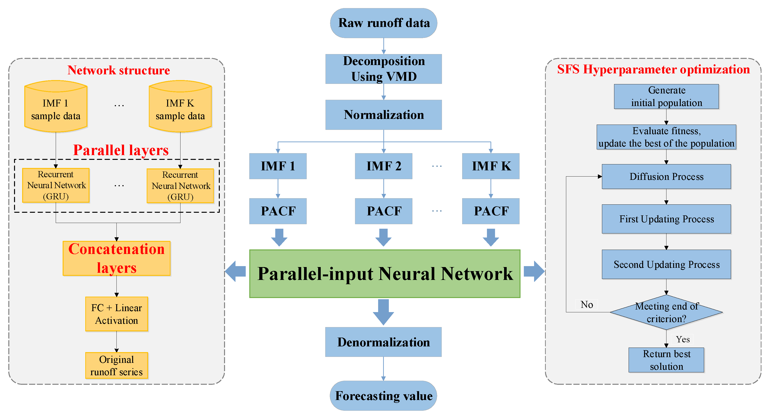
Figure 3.
Structure of the constructed parallel-input neural network.

Figure 4.
Study area and location of the two hydrological stations in Upper Yangtze River Basin.

Figure 5.
Prediction results and residual of different methods for the Pingshan station. (a) AR model prediction residual; (b) BP model prediction residual; (c) LSTM model prediction residual; (d) GRU model prediction residual; (e) VMD-LSTM (DPR) model prediction residual; (f) VMD-GRU (DPR) model prediction residual; (g) VMD-GRU-SFS (DPR) model prediction residual; (h) Proposed model prediction residual.

Figure 6.
Prediction results and residual of different methods for the Yichang station. (a) AR model prediction residual; (b) BP model prediction residual; (c) LSTM model prediction residual; (d) GRU model prediction residual; (e) VMD-LSTM (DPR) model prediction residual; (f) VMD-GRU (DPR) model prediction residual; (g) VMD-GRU-SFS (DPR) model prediction residual; (h) Proposed model prediction residual.

Figure 7.
Scatter plots of different methods for the Pingshan station. (a) AR model; (b) BP model; (c) LSTM model; (d) GRU model; (e) VMD-LSTM (DPR) model; (f) VMD-GRU (DPR) model; (g) VMD-GRU-SFS (DPR) model; (h) Proposed model.
Figure 7.
Scatter plots of different methods for the Pingshan station. (a) AR model; (b) BP model; (c) LSTM model; (d) GRU model; (e) VMD-LSTM (DPR) model; (f) VMD-GRU (DPR) model; (g) VMD-GRU-SFS (DPR) model; (h) Proposed model.

Figure 8.
Scatter plots of different methods for the Yichang station. (a) AR model; (b) BP model; (c) LSTM model; (d) GRU model; (e) VMD-LSTM (DPR) model; (f) VMD-GRU (DPR) model; (g) VMD-GRU-SFS (DPR) model; (h) Proposed model.
Figure 8.
Scatter plots of different methods for the Yichang station. (a) AR model; (b) BP model; (c) LSTM model; (d) GRU model; (e) VMD-LSTM (DPR) model; (f) VMD-GRU (DPR) model; (g) VMD-GRU-SFS (DPR) model; (h) Proposed model.

Figure 9.
Improvement rates in terms of statistical Indexes in the testing stage of the proposed method for runoff forecasts at the Pingshan station, as compared with the different models. (a) RMSE/NRMSE improvement rate; (b) MAPE improvement rate; (c) NSE improvement rate.
Figure 9.
Improvement rates in terms of statistical Indexes in the testing stage of the proposed method for runoff forecasts at the Pingshan station, as compared with the different models. (a) RMSE/NRMSE improvement rate; (b) MAPE improvement rate; (c) NSE improvement rate.

Figure 10.
Improvement rates in terms of statistical indexes in the testing stage of the proposed method for runoff forecasts at the Yichang station, as compared with the different models. (a) RMSE/NRMSE improvement rate; (b) MAPE improvement rate; (c) NSE improvement rate.
Figure 10.
Improvement rates in terms of statistical indexes in the testing stage of the proposed method for runoff forecasts at the Yichang station, as compared with the different models. (a) RMSE/NRMSE improvement rate; (b) MAPE improvement rate; (c) NSE improvement rate.

Figure 11.
Training time of different methods for the two hydrological station.

Figure 12.
Scatter fitting plots for test sets using VMD-GRU-SFS (DPR) and the proposed method for 1, 2 and 3-step ahead forecast at Yichang station. (a) VMD-GRU-SFS (DPR) model; (b) The proposed method.
Figure 12.
Scatter fitting plots for test sets using VMD-GRU-SFS (DPR) and the proposed method for 1, 2 and 3-step ahead forecast at Yichang station. (a) VMD-GRU-SFS (DPR) model; (b) The proposed method.

Table 1.
Optimal input variables of each IMF for Yichang Hydrological station.
| IMFs | Input Variables | Numbers of Input |
|---|---|---|
| IMF1 | Xt-1~Xt-11, Xt-14, Xt-15, Xt-17~Xt-19 | 16 |
| IMF2 | Xt-1~Xt-11, Xt-14~Xt-19 | 17 |
| IMF3 | Xt-1~Xt-10, Xt-12, Xt-14, Xt-17~Xt-22 | 18 |
| IMF4 | Xt-1~Xt-10, Xt-14, Xt-15, Xt-17, Xt-20~Xt-23, Xt-27, Xt-29 | 19 |
| IMF5 | Xt-2, Xt-4~Xt-9, Xt-13~Xt-16, Xt-18~Xt-20, Xt-24, Xt-27 | 16 |
| IMF6 | Xt-1~Xt-8, Xt-10~Xt-12, Xt-16, Xt-20, Xt-23, Xt-35 | 15 |
| IMF7 | Xt-1~Xt-12, Xt-16~Xt-20, Xt-23~Xt-28, Xt-30~Xt-32, Xt-36 | 27 |
| IMF8 | Xt-1~Xt-3, Xt-5, Xt-6, Xt-8, Xt-13, Xt-14, Xt-16, Xt-25~Xt-29 | 14 |
Table 2.
Summary of the parameter configuration of forecasting Model.
| Station | Layers | Hidden Layers | Hidden Nodes | Activation Function | Loss Function | Optimizer | Epochs | Batch Size |
|---|---|---|---|---|---|---|---|---|
| Pingshan | multi-input layers | 2 | 22 | softsign | mse | adam | 20 | 8 |
| 29 | softsign | |||||||
| concatenation layers | 2 | 37 | softsign | |||||
| 12 | linear | |||||||
| Yichang | multi-input layers | 2 | 27 | softsign | mse | adam | 20 | 8 |
| 43 | softsign | |||||||
| concatenation layers | 2 | 34 | softsign | |||||
| 19 | linear |
Table 3.
Results of different forecasting methods for the Pingshan station.
| Model | Training | Testing | ||||||
|---|---|---|---|---|---|---|---|---|
| RMSE | NRMSE | MAPE | NSE | RMSE | NRMSE | MAPE | NSE | |
| AR | 1464.36 | 10.89 | 24.2 | 0.835 | 1771.89 | 13.18 | 25.6 | 0.791 |
| BP | 1378.41 | 10.26 | 20.9 | 0.854 | 1724.55 | 12.83 | 20.3 | 0.805 |
| LSTM | 1302.25 | 9.69 | 13.7 | 0.869 | 1688.15 | 12.56 | 18.4 | 0.813 |
| GRU | 1282.78 | 9.54 | 15.9 | 0.873 | 1700.87 | 12.65 | 19.3 | 0.811 |
| VMD-LSTM (DPR) | 1228.62 | 9.14 | 21.8 | 0.883 | 1496.11 | 11.13 | 21.7 | 0.853 |
| VMD-GRU (DPR) | 1178.06 | 8.76 | 20.2 | 0.892 | 1449.76 | 10.79 | 19.7 | 0.862 |
| VMD-GRU-SFS (DPR) | 1134.25 | 8.44 | 19.2 | 0.901 | 1399.51 | 10.41 | 18.9 | 0.871 |
| Proposed | 1056.28 | 7.86 | 19.6 | 0.914 | 1310.62 | 9.75 | 17.9 | 0.887 |
Table 4.
Results of different forecasting methods for the Yichang station.
| Model | Training | Testing | ||||||
|---|---|---|---|---|---|---|---|---|
| RMSE | NRMSE | MAPE | NSE | RMSE | NRMSE | MAPE | NSE | |
| AR | 3946.35 | 10.38 | 19.9 | 0.852 | 4433.03 | 11.67 | 22.9 | 0.757 |
| BP | 3785.58 | 9.96 | 18.3 | 0.863 | 4343.23 | 11.43 | 22.1 | 0.771 |
| LSTM | 3562.45 | 9.37 | 14.7 | 0.879 | 4204.73 | 11.06 | 20.1 | 0.784 |
| GRU | 3469.44 | 9.13 | 13.9 | 0.885 | 4098.51 | 10.78 | 17.6 | 0.794 |
| VMD-LSTM (DPR) | 3241.23 | 8.53 | 18.2 | 0.899 | 3828.96 | 10.08 | 20.9 | 0.821 |
| VMD-GRU (DPR) | 3202.11 | 8.43 | 15.4 | 0.902 | 3670.41 | 9.66 | 20.1 | 0.834 |
| VMD-GRU-SFS (DPR) | 2917.92 | 7.68 | 16.9 | 0.918 | 3414.16 | 8.98 | 19.1 | 0.856 |
| Proposed | 2943.65 | 7.75 | 16.6 | 0.917 | 3145.08 | 8.28 | 16.2 | 0.878 |
Table 5.
Results of different forecasting methods for the Yichang station.
| Steps | VMD-GRU-SFS(DPR) | The Proposed | ||||||
|---|---|---|---|---|---|---|---|---|
| RMSE | NRMSE | MAPE | NSE | RMSE | NRMSE | MAPE | NSE | |
| 1-step-ahead | 3414.16 | 8.98 | 19.1 | 0.856 | 3145.08 | 8.28 | 16.2 | 0.878 |
| 2-step-ahead | 3913.61 | 10.30 | 23.7 | 0.812 | 3405.01 | 8.96 | 20.9 | 0.857 |
| 3-step-ahead | 4368.91 | 11.50 | 29.9 | 0.765 | 3905.09 | 10.28 | 21.1 | 0.813 |
Publisher’s Note: MDPI stays neutral with regard to jurisdictional claims in published maps and institutional affiliations. |
© 2021 by the authors. Licensee MDPI, Basel, Switzerland. This article is an open access article distributed under the terms and conditions of the Creative Commons Attribution (CC BY) license (https://creativecommons.org/licenses/by/4.0/).
Share and Cite
MDPI and ACS Style
Xu, Z.; Zhou, J.; Mo, L.; Jia, B.; Yang, Y.; Fang, W.; Qin, Z. A Novel Runoff Forecasting Model Based on the Decomposition-Integration-Prediction Framework. Water 2021, 13, 3390. https://doi.org/10.3390/w13233390
AMA Style
Xu Z, Zhou J, Mo L, Jia B, Yang Y, Fang W, Qin Z. A Novel Runoff Forecasting Model Based on the Decomposition-Integration-Prediction Framework. Water. 2021; 13(23):3390. https://doi.org/10.3390/w13233390
Chicago/Turabian StyleXu, Zhanxing, Jianzhong Zhou, Li Mo, Benjun Jia, Yuqi Yang, Wei Fang, and Zhou Qin. 2021. "A Novel Runoff Forecasting Model Based on the Decomposition-Integration-Prediction Framework" Water 13, no. 23: 3390. https://doi.org/10.3390/w13233390
Note that from the first issue of 2016, this journal uses article numbers instead of page numbers. See further details here.