Sandtank-ML: An Educational Tool at the Interface of Hydrology and Machine Learning

Abstract

Hydrologists and water managers increasingly face challenges associated with extreme climatic events. At the same time, historic datasets for modeling contemporary and future hydrologic conditions are increasingly inadequate. Machine learning is one promising technological tool for navigating the challenges of understanding and managing contemporary hydrological systems. However, in addition to the technical challenges associated with effectively leveraging ML for understanding subsurface hydrological processes, practitioner skepticism and hesitancy surrounding ML presents a significant barrier to adoption of ML technologies among practitioners. In this paper, we discuss an educational application we have developed—Sandtank-ML—to be used as a training and educational tool aimed at building user confidence and supporting adoption of ML technologies among water managers. We argue that supporting the adoption of ML methods and technologies for subsurface hydrological investigations and management requires not only the development of robust technologic tools and approaches, but educational strategies and tools capable of building confidence among diverse users.

1. Introduction

Water is a driving force for extreme events, which are increasing in frequency and severity at an alarming rate. As of September 2021, there have been 18 weather and climate disaster events, each costing over one billion dollars [1]. California had its worst fire season on record in 2020, with the 2021 season expected to surpass this dire benchmark [2]. Simultaneously, over half of the U.S. is experiencing drought conditions [3], including the Colorado River, which is at risk of downstream user curtailments [4]. These extreme events put life, property, infrastructure, livelihoods, and our collective water future at risk. Researchers across scientific disciplines agree that climate change will drive the continued increase in the degree and frequency of extreme events [5].

Alongside the increased prevalence and intensity of extreme events, scientists and decision makers face an additional challenge: the historical datasets traditionally used for modeling, prediction, and decision making are no longer adequate for understanding future conditions. These datasets are increasingly unrepresentative of current and future conditions, leaving us without the right information to answer vital questions about water quantities, availability, and movement in systems. This lack of relevant information drives the need for new technologies and approaches to understand, model, and predict hydrological conditions in a way that enables the effective management of water. Our collective environment is changing and the water resources that are intertwined with these environments are changing, so accessible, customizable tools to evaluate these systems in flux are critical. Machine learning is one promising technological tool for navigating the challenges of understanding and managing contemporary hydrological systems.

Machine learning (ML) is a type of artificial intelligence (AI) that relies on the introduction of large amounts of data to computer systems, allowing them to “learn” through experience [6]. ML is a pervasive tool in our society, driving technology forward. You will find ML playing a role in anything from self-driving cars to medical image recognition and beyond. Within the realm of hydrology, ML is being mobilized to improve hydrological forecasting within the context of unprecedented climatic shifts. For example, Cai et al. (2021) explored the impact of catchment physical properties on ML performance for groundwater level prediction [7]. They found that various hydrometeorological and geological characteristics impacted the simulation accuracy and recommended continued work to increase trust in the use of ML technology in hydrology. Frame and colleagues (2021) aimed to understand whether process-based models are more reliable for predicting extreme events (in this case, streamflow) as compared to data-driven models [8]. This work demonstrated that under these testing conditions the data-driven models (including physics-informed ML model and purely ML model) performed better than process-based models at predicting peak flows under a variety of conditions, including extreme events. Other recent ML applications in hydrology include well sample mean age prediction [9], multi-year El Niño-Southern Oscillation (ENSO) forecasting [10], prediction of point discharge observation timing [11], and prediction of subsurface permeability from stream discharge [12]. Although these findings support the significant potential of ML in hydrology, researchers caution that more work needs to be done to better understand the black box of ML and how to apply it in physically meaningful ways. While ML technologies are being adopted in some realms of hydrology, the learning curve to apply such approaches is steep and the required resources are often prohibitive for water managers on the ground. This creates barriers to the adoption of ML technologies among those making decisions regarding water management practices.

The HydroGEN project aims to harness the power of ML to improve our understanding of contemporary hydrological systems and processes and associated water management systems by doing two things. First, we are working to improve ML technologies. Our web-based platform is designed to generate customized hydrologic scenarios that can be easily manipulated by users to address scale, observations, and locations that are relevant to their needs. HydroGEN trains ML models on synthetic datasets generated by physically-based hydrologic models combined with observations. Unlike the commonly used data-driven methods, this approach allows the ML model to be trained with events that are more extreme than what has historically been observed and to simulate poorly observed variables like soil moisture and groundwater depth.

Second, we are developing a suite of educational and training tools to make ML and the role it can play in water management systems more accessible and relevant, in turn increasing the adoption and utilization of ML technologies among water managers. Despite the increasing importance and utility of ML, user interviews we conducted with educators and hydrologists indicated that there are few accessible educational tools and resources that engage with machine learning in general and even fewer that exist at the interface of hydrology and machine learning (an emerging exception to this are the educational resources produced by the National Science Foundation AI Institute for Research on Trustworthy AI in Weather, Climate and Coastal Oceanography (https://www.ai2es.org/products/education/ (accessed on 25 October 2021). Moreover, existing open access ML educational tools often require high levels of base knowledge and/or a significant level of time committed by the user in order to progress through curricula (for example, see: https://www.tensorflow.org/resources/learn-ml (accessed on 25 October 2021). While these educational tools are useful for helping individuals gain proficiency and understanding in the foundational ML concepts and practices, they are in many cases too time intensive and more in-depth than is needed for supporting adoption of ML among water managers. In response to a gap in the education and training ecosystem around easily accessible and useable ML educational tools, our team has developed a web-based educational application, Sandtank-ML, that allows users to gain an understanding of basic ML concepts, as well as the way in which ML can be used to understand and address hydrological processes and challenges.

In the next section, we provide an overview of Sandtank-ML before discussing how this application will be utilized within the context of the HydroGEN project to build confidence and support adoption of ML-based technologies among water managers and the public.

2. Materials and Methods

2.1. Sandtank-ML Capabilities and User Workflow

Sandtank-ML builds upon an already existing educational tool created by members of our research team called the ParFlow Sandtank. The ParFlow Sandtank (https://sandtank.hydroframe.org (accessed on 25 October 2021)), is an interactive computer simulation of a physical aquifer model. The ParFlow Sandtank allows users to explore the subsurface, controlling various inputs, visualizing outputs in real time, and using tools to evaluate factors that impact real hydrogeological systems. Using the output of the ParFlow Sandtank as the prediction goal, Sandtank-ML allows users to run different ML models and manipulate training sets and other components to explore how particular decisions impact model accuracy. The goal of the application is to help users gain an understanding of basic ML approaches and processes, while building confidence in ML as a tool that can be used to understand and address real-world environmental issues. Sandtank-ML can be used with both water managers and students to increase knowledge of basic ML concepts and processes, building confidence and supporting adoption of the technology.

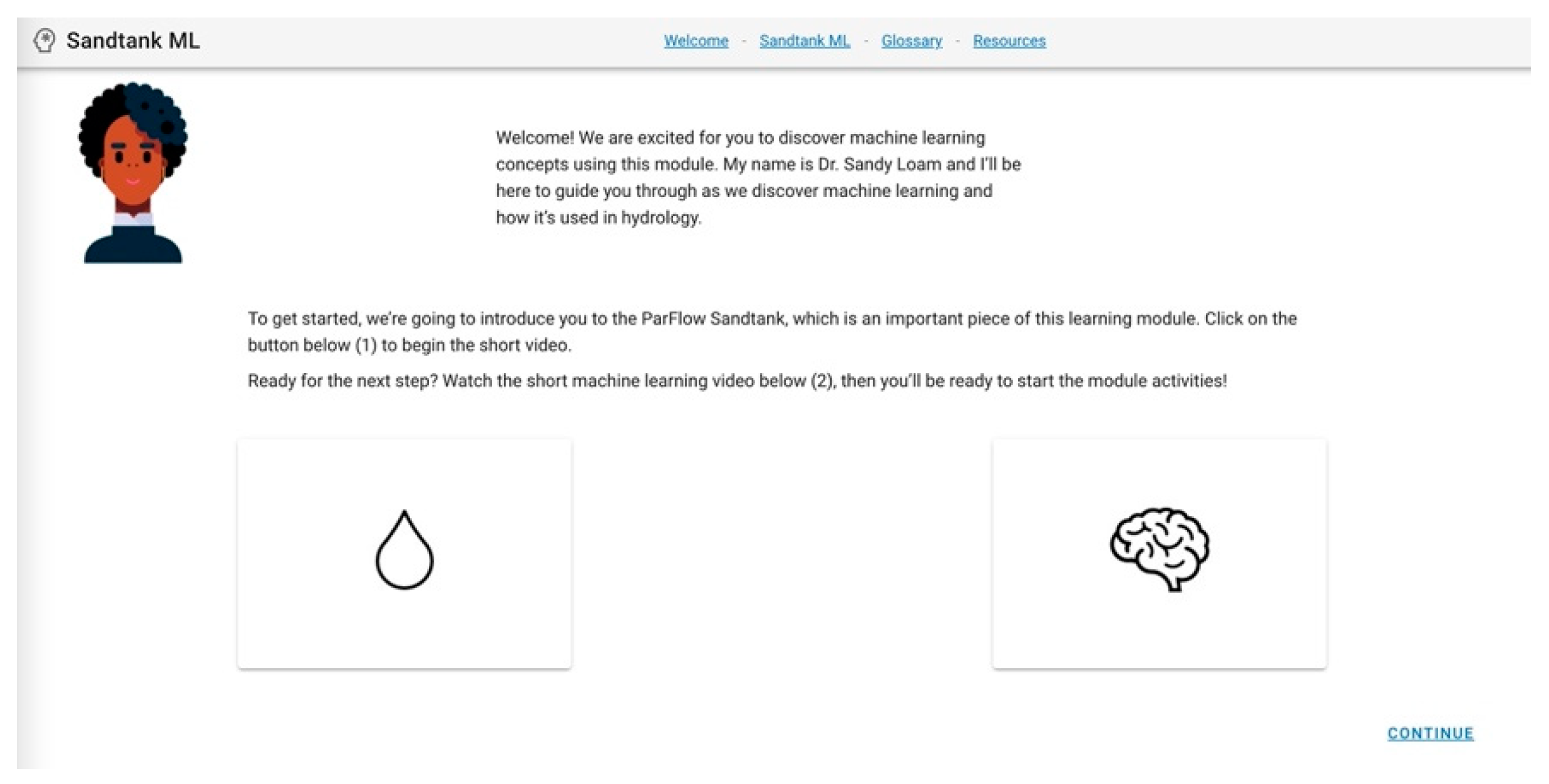
Users can access Sandtank-ML via: https://sandtank-ml.hydroframe.org (accessed on 25 October 2021). This URL directs users to the welcome page (Figure 1), where you are introduced to Dr. Sandy Loam, who will guide users through the application and provide additional information as needed. Because we are interested in using this application to both promote understanding and adoption of ML and broaden understanding of who engages in computer and geoscience education, we strategically designed the main character of the app to be a woman of color. Existing data indicate that only approximately 15% of individuals in the computer science workforce are people of color [13] and research has repeatedly indicated that the representations of scientists and engineers are key to shaping differential rates of entry and retention in STEM fields and careers [14,15,16]. Similarly, Geoscience fields continue to collectively be the least diverse in STEM [17]. Dr. Loam works to introduce a non-typical representation of a computer scientist and geoscientist. The welcome page houses two videos (under development): a video that introduces the ParFlow Sandtank, which is a foundational piece of Sandtank-ML; and an introductory machine learning video, that will provide users with the background information and context to successfully use the application (Figure 1).

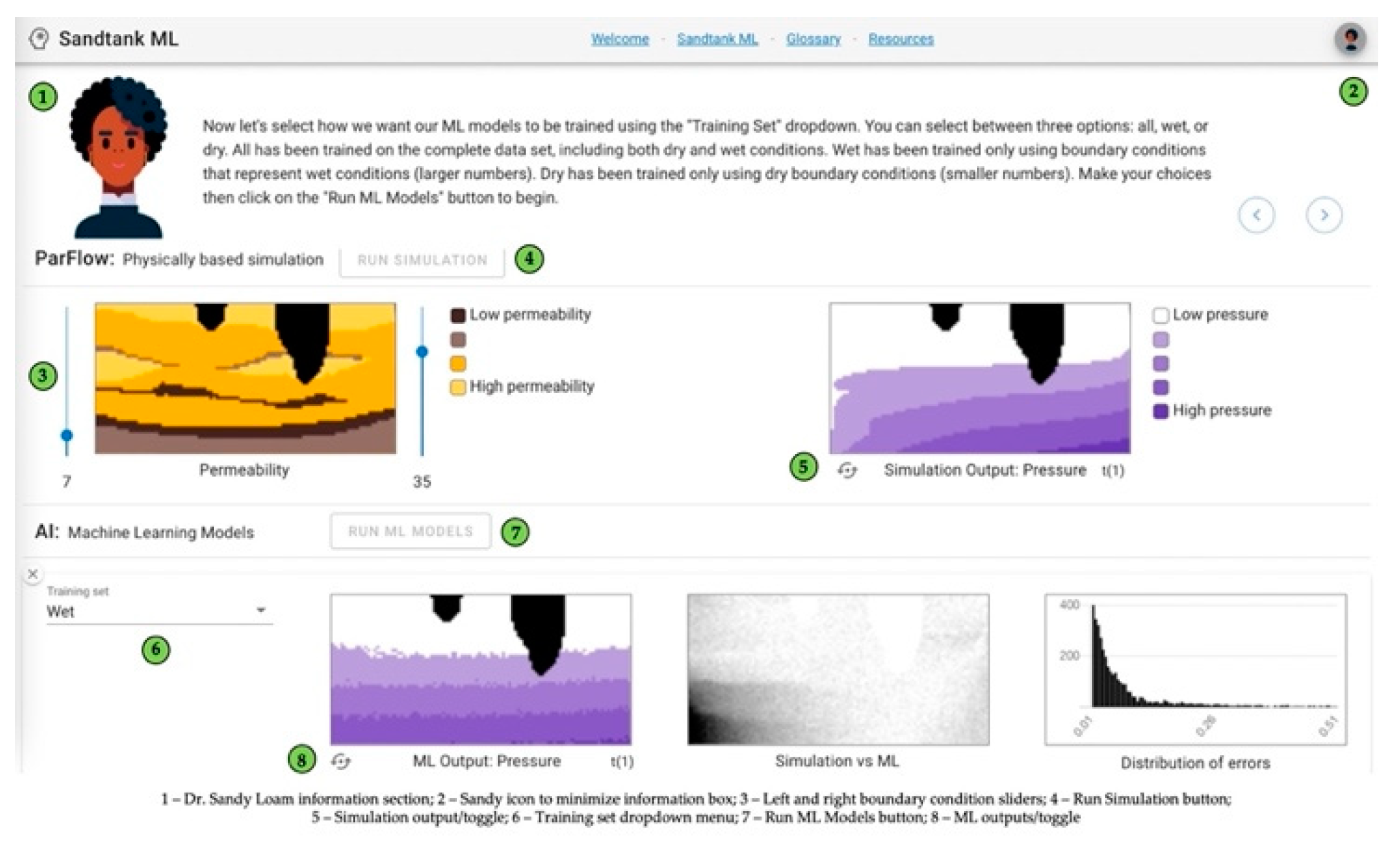
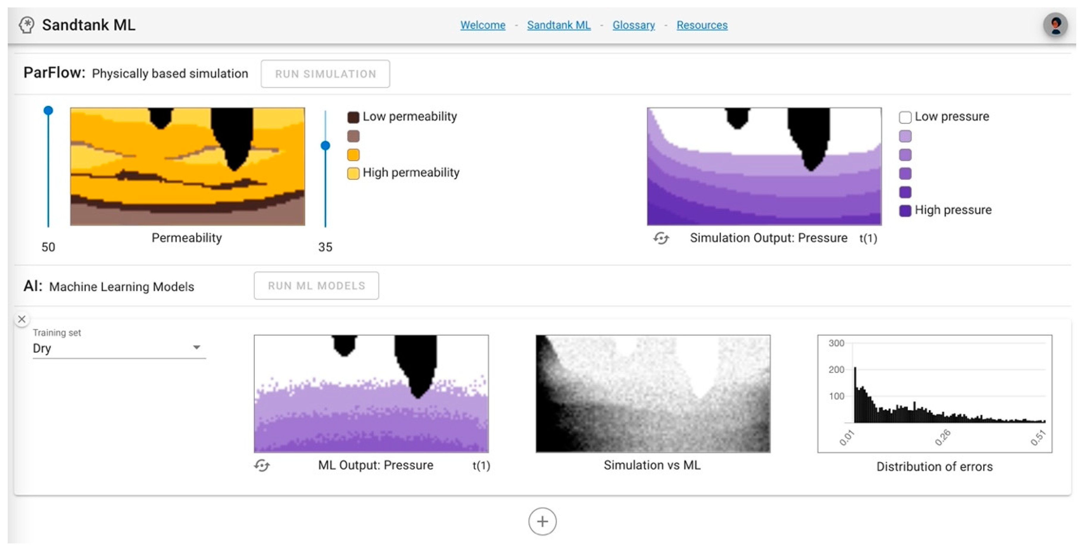
Once users have completed the welcome activities, they are directed to the main application page by clicking on the Sandtank ML tab in the navigation bar. The features of this page are displayed in Figure 2. On this page, users are again greeted by Dr. Loam, who provides context and instructions, which can be minimized if the user desires. Users are directed to the ParFlow section of the application, where they have the capability to adjust boundary conditions by dragging the sliders up or down to change the values. Higher values represent wet conditions, while lower values represent dry conditions. Once the sliders have been set, users are prompted to click on the Run Simulation button, which will begin the physically based simulation using the provided input. ParFlow, an open-source parallel watershed flow model, is used in this step to generate hydrologic simulations [18,19,20,21]. After a few moments, the simulation generates a pressure output (represented by purple) and a saturation output (represented by blue), which you can toggle between using the icon in the lower left corner of the image. These simulation outputs then become the target outputs for the machine learning models that will be used.

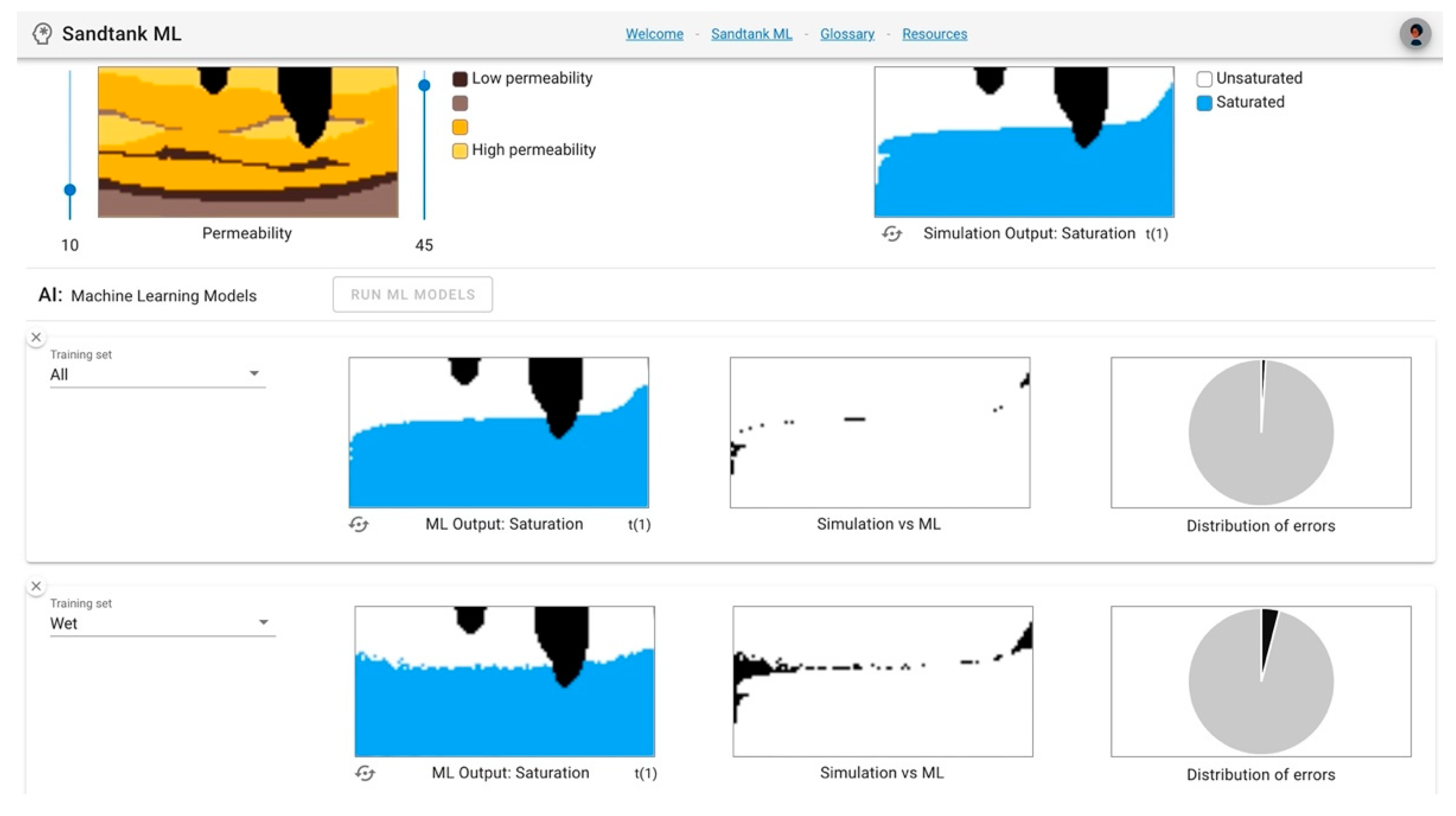
Users are then directed to the AI section, where the plus button can be clicked to add ML models. The first decision point is the training set, which allows the user to decide what type of dataset the ML model uses to “learn.” Our team identified this step as vital to understand in the overall ML process and developed this option specifically to enhance user understanding and trust in the training process. The training selections include all, wet, or dry. The all option provides a complete dataset, including both dry and wet conditions. The wet option trains the ML model using only boundary conditions that represent wet conditions (larger values). The dry choice offers the ML model only dry boundary conditions (smaller values) for training. Once users have made training set decisions, they are prompted to click the Run ML Models button to allow the machine learning process to begin. This step in the process represents a number of iterations of training and validation that each ML model undergoes before it presents the output prediction for analysis.

2.2. Sandtank-ML Outputs and Analysis

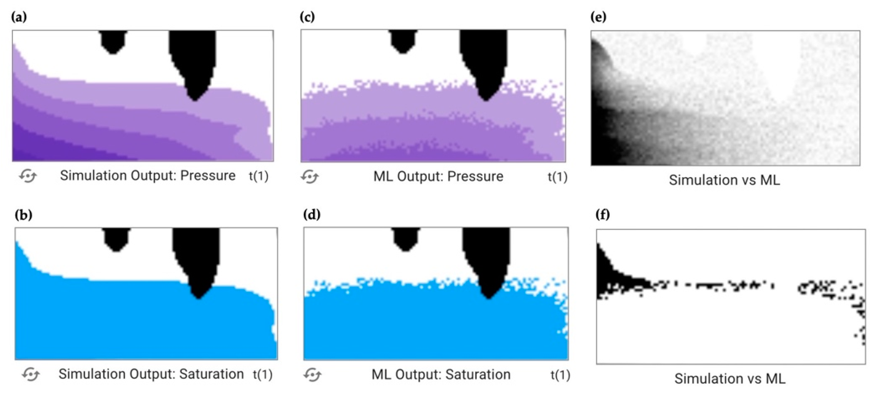
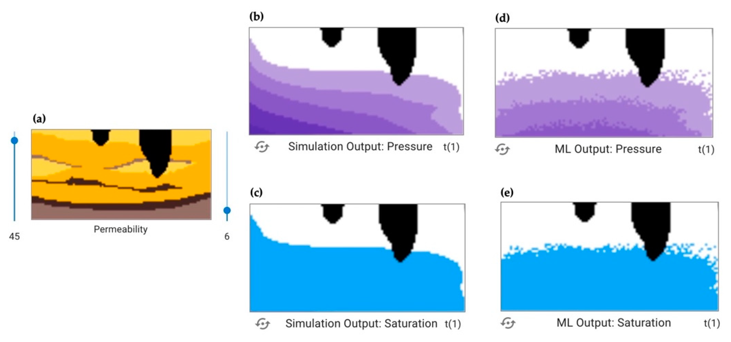
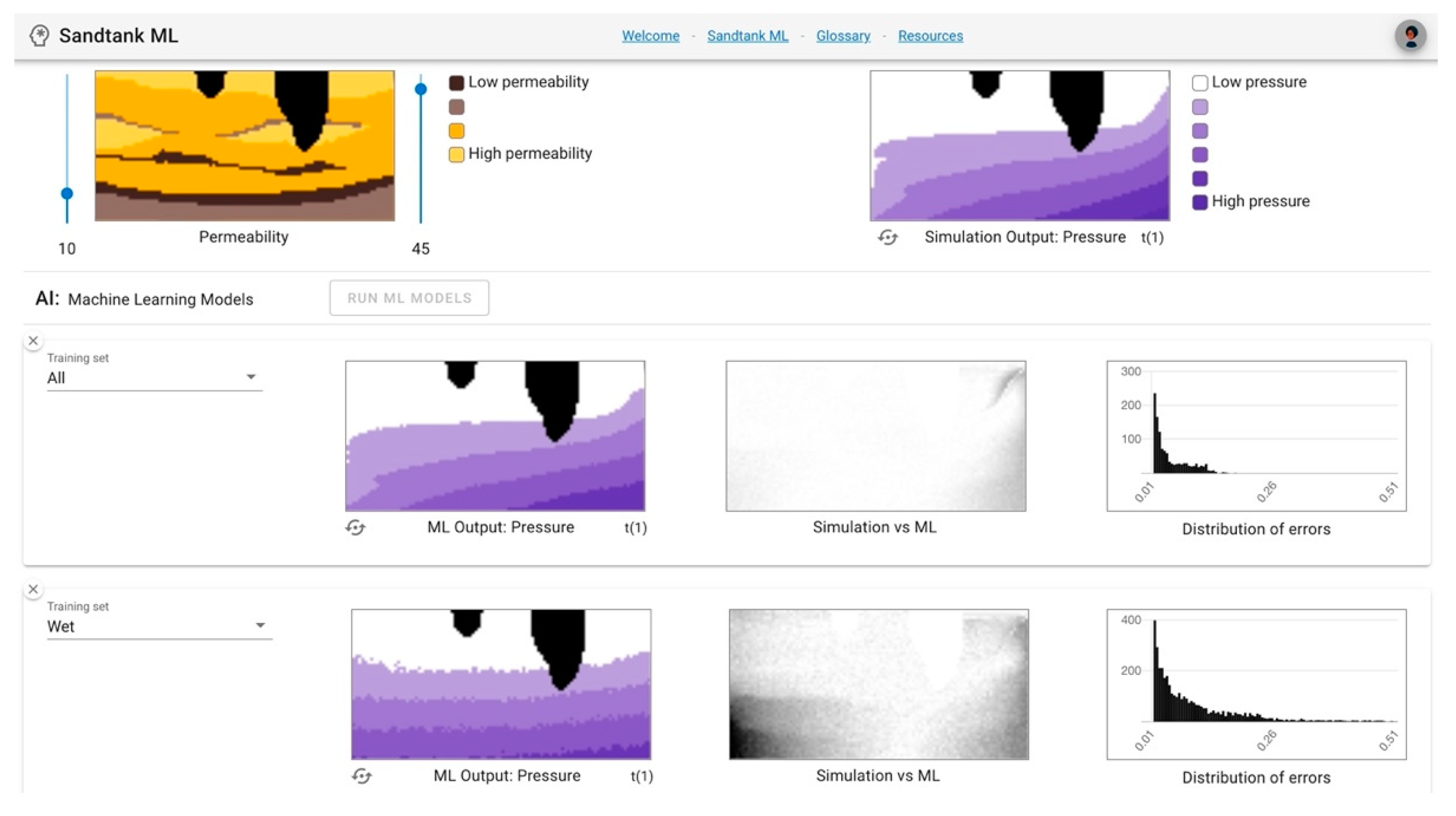
Once users have generated ML outputs, there is an opportunity to compare and analyze outputs from the ML models to the physically based simulation, which is the goal of the ML predictive model. The left column output, “ML output: Pressure/Saturation”, allows users to visually compare the predicted output to the simulation output, where a pixelated or mismatching image represents less agreement between the simulation and the ML. 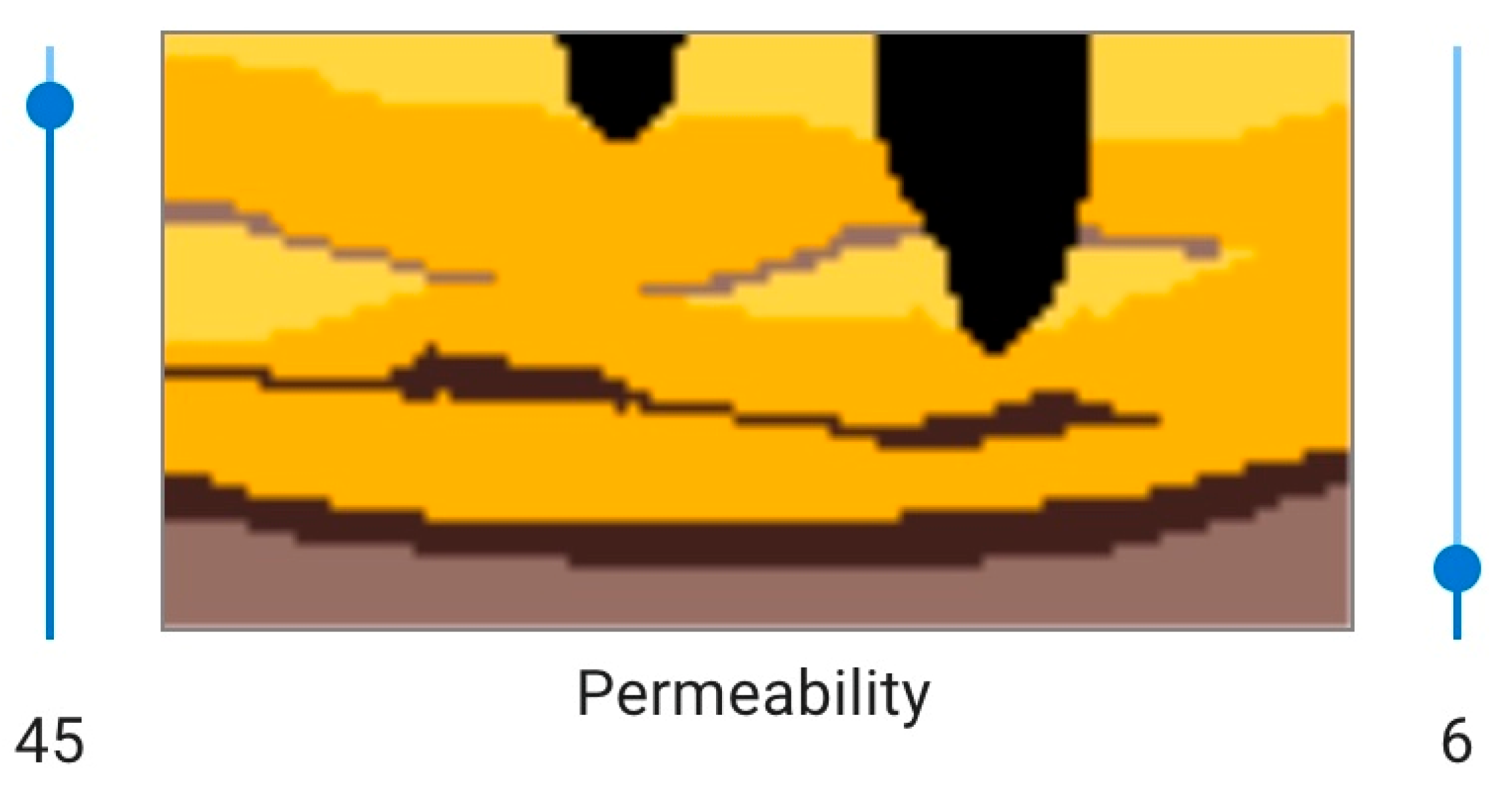For example, Figure 3 shows (a) the input conditions for the simulation, (b) the “goal” simulation output for pressure, (c) the “goal” simulation output for saturation, (d) the ML pressure output using a dry training set, and (e) the ML saturation output using a dry training set. It is clear that the ML outputs do not accurately represent the simulation results. The image shapes do not align well and there is significant pixelation (panels d, e) which indicates that the ML model would need more training (with potentially more data or more representative data) to achieve better results.

In the center column, the mathematical difference between the simulation and the ML is presented as “Simulation vs. ML”. A pixel that is black represents a greater difference between the simulation and ML, while a white pixel represents a smaller difference. Figure 4 continues the example from Figure 3, adding in panels (e) and (f) which show the difference column for pressure (e) and saturation (f) outputs. Visual inspection allows the user to recognize that the ML outputs in panels (c) and (d) do not accurately represent the goal images in panels (a) and (b), as discussed above. Panels (e) and (f) allow users to add a layer of numerical value to that analysis. In panel (e), the dark pixels, ones with greater difference between the simulation and the ML, are mostly on the left side of the image. In this run, the left boundary condition was set to 45, a large value, which represents wet conditions (Figure 3). Since this ML model was trained using a dry dataset, it was not given data that represented wet conditions, so did poorly at predicting this specific outcome. A similar effect can be observed in panel (f) in relation to saturation, where there is greater difference on the wet boundary condition side of the image.

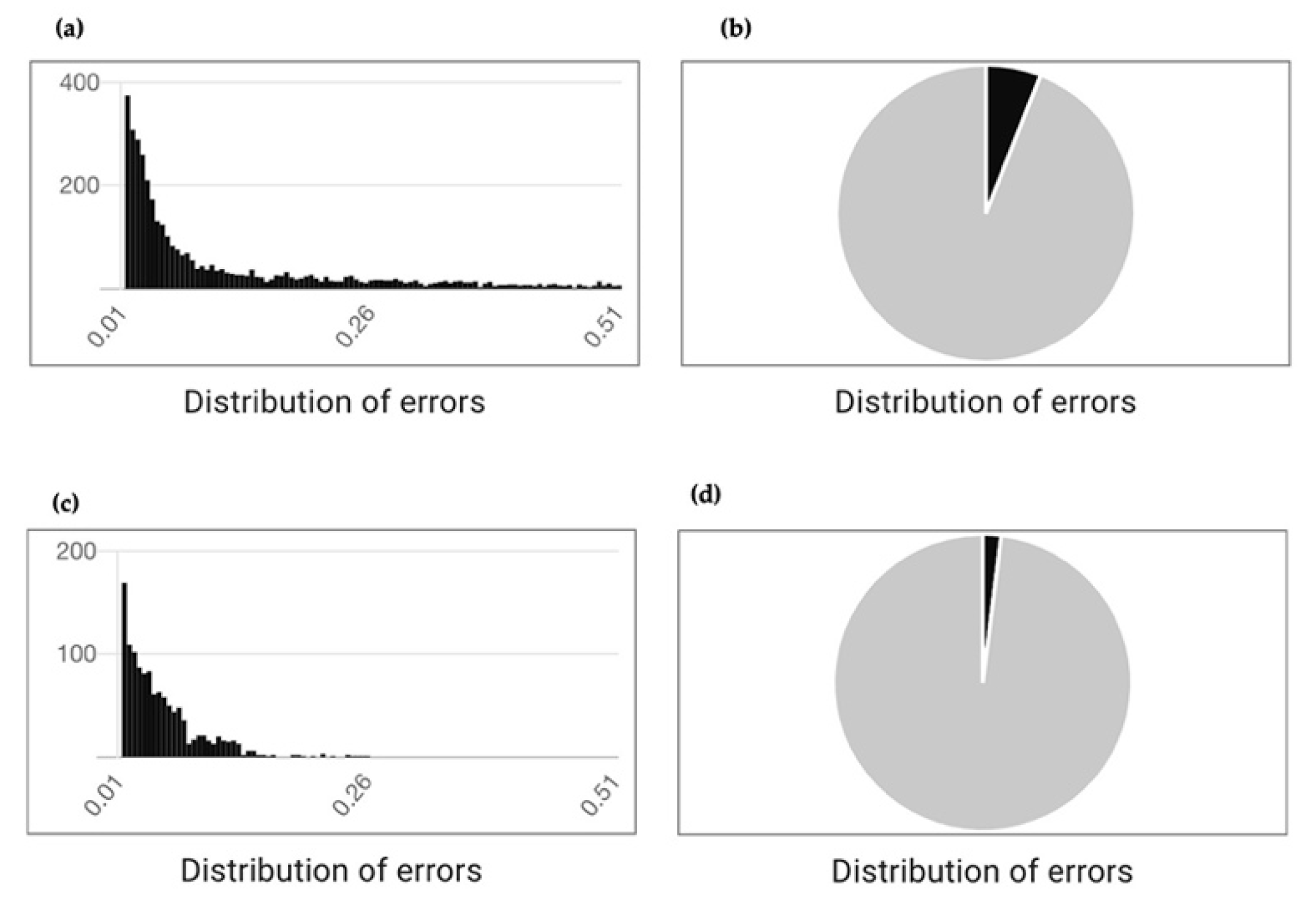
Finally, in the right column of the application ML outputs, the distribution of errors is presented. Figure 5 displays the pressure (a) and saturation (b) outputs for the same example highlighted in Figure 3 and Figure 4 (a dry dataset), along with pressure (c) and saturation (d) distribution of errors for an ML model trained using the all dataset (i.e., both wet and dry data). Upon visual analysis, there is an evident decrease in the number of errors, as well as the amount of error from the ML model training with the dry dataset as compared to the ML model trained using both wet and dry data. These ML outputs build a foundation for development of educational and training resources to achieve our goal of increased understanding, accessibility, and adoption of our technology.

Importantly, Sandtank-ML does not aspire to educate users on precisely how the full HydroGEN application works. Rather, the goal is to provide users with a base-level understanding of the foundational concepts and processes central to how ML is utilized within the context of hydrological forecasting so that they gain confidence in the process and technology.

2.3. Hydrology and ParFlow

Numerical modeling has been used to explore the role of groundwater, soil moisture dynamics, and overland flow. This work builds on the integrated hydrology model, ParFlow [22]. ParFlow [23] simulates fully coupled unsaturated, saturated and overland flow [19,20,24]. ParFlow has been used widely in prior work to study the effects of heterogeneity on flow, runoff, and land-energy balance [25,26,27,28,29,30]. ParFlow is an open-source software platform [31] which is freely available and runs on a wide range of systems from laptop to supercomputer. Here, we use a specific model built using the ParFlow platform designed to replicate the popular sand tank physical hydrology model. This model, shown in Figure 6, simulates saturated and unsaturated water flow using the two dimensional Richards’ equation and integrated surface flow for the river. When the river is switched to the lake, the surface outflow is turned off and pressures can rise and fall with the lake level. This model runs in real time, in a container, in the application.

2.4. Machine Learning

There are challenges and opportunities utilizing machine learning to emulate groundwater evolution. The challenges include few training samples, out-of-distribution prediction, approximated uncertainties, and prediction over various time scales. However, we are enticed by the capabilities that include large, open datasets, new emulators, improved data assimilation, and observation-based emulators.

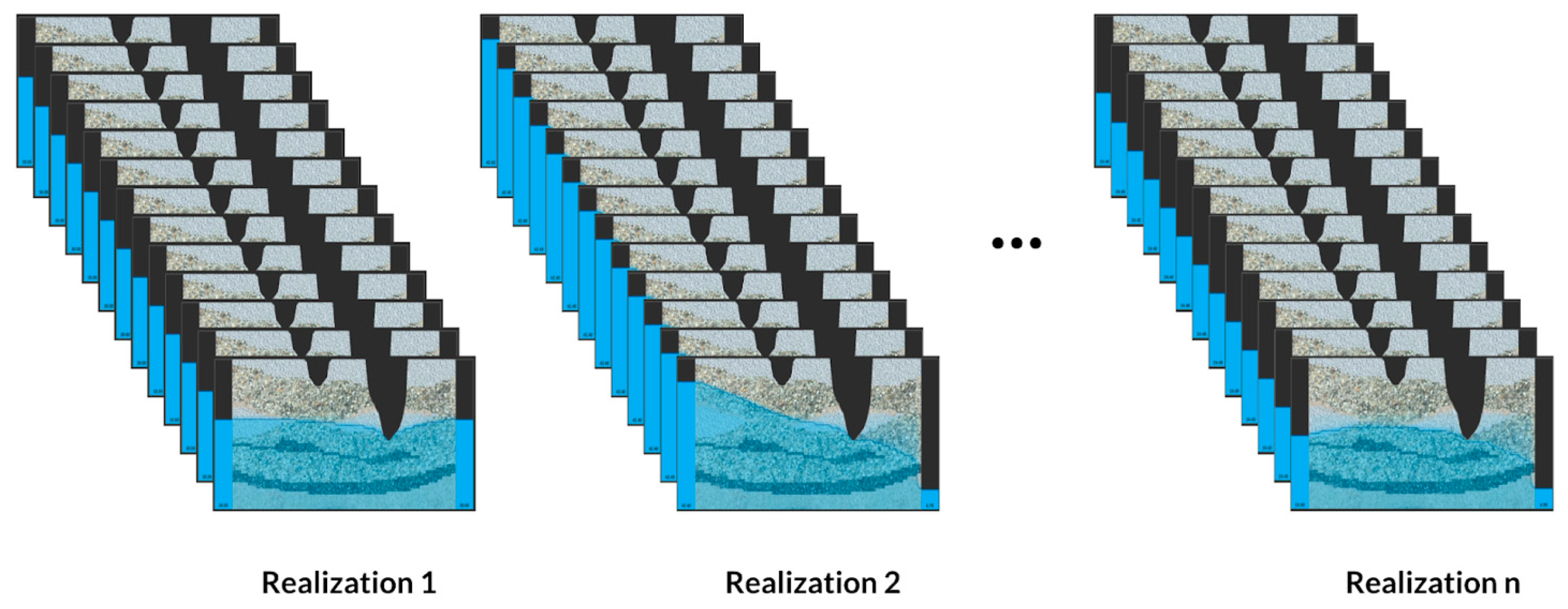
It is hard to fathom that terabytes of groundwater simulation data results in too few training samples, but the number of samples over the adjustable parameters spanning dimension is often small. We addressed this challenge in two ways: reduced spatial dimensions and limited adjustable parameters. Reducing the simulator from three-dimensions to two-dimensions allowed us to balance the size of the simulation data results (Figure 7). Limiting the adjustable parameters to the right and the left boundary conditions condensed the spanning dimension of the emulation space. These two assumptions balanced our emulator exploration, yielding adequate training data.

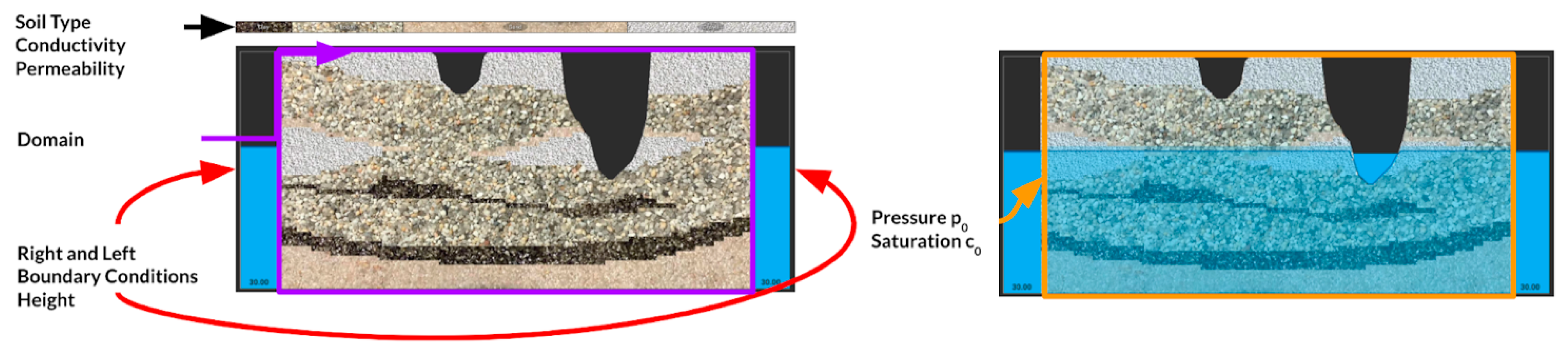
Although we built the Sandtank simulator to accept a variety of soil configurations, we held to the default configuration for our initial exploration (Figure 8). Additionally, we fixed the initial pressure and saturation conditions. In the end, we allow two parameters to vary, the right and the left boundary conditions. This numerical setup allowed us to examine both in-distribution and out-of-distribution prediction by short-sheeting the generated range of one or both of the adjustable parameters. Finally, we restricted our prediction time-scale to solely the next time step. The schematic of these conditions can be visualized in Figure 8.

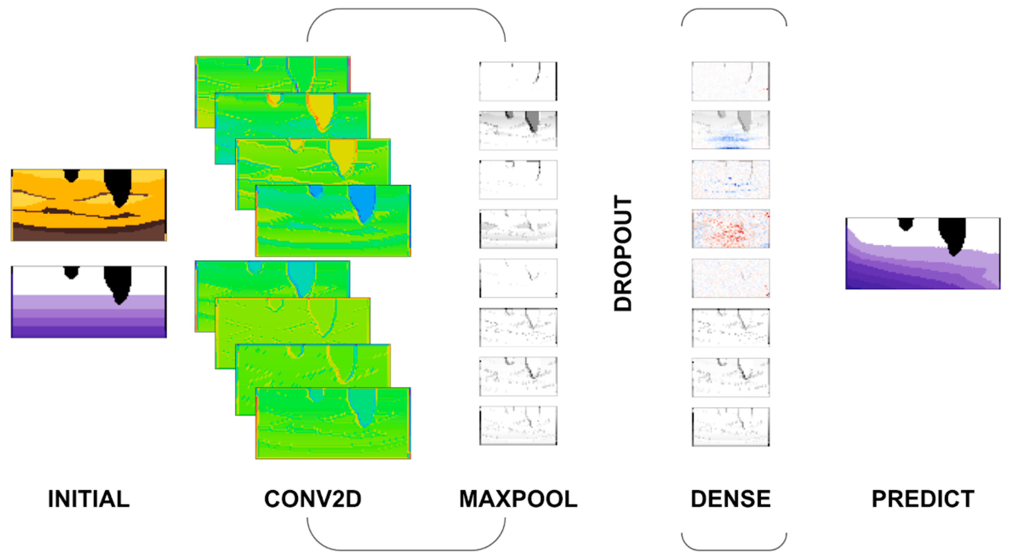
To predict pressure at the next step, we train a Convolutional Neural Network (CNN), which has proven very effective in image recognition and classification (Figure 9). Instead of classification, we reformulated the network for regression similar to what Ronneberger et al. implemented for U-net [32]. A CNN is a simple deep learning algorithm that applies a filter to input to create a map of features used to summarize the presence of these features in the data.

As Figure 9 shows, our network uses a two-dimensional convolutional layer (CONV2D) followed by a pooling layer (MAXPOOL) to downsample the features. MAXPOOL removes the position and orientation bias while reducing the overall size of the final dense layer (DENSE). These two elements are a common pattern for CNN and may be repeated one or more times to detect features at different scales. Next, we introduce a dropout layer (DROPOUT) to prevent our model from overfitting by randomly setting some outgoing edges to 0 at each update of the training phase. The uncertainties of our numerical model are constructed naturally as we move from a physical model to a mathematical model through to a computer model using simplifying assumptions. So, a dropout layer can be used to approximate uncertainties [33] for neural networks (NN). Finally, the dense layer uses L1Loss to drive the training for regression.

Sandtank-ML uses Pytorch and PyTorch Lighting to implement the network and facilitate distributed training leveraging multiple GPUs. Our Sandtank, ParFlow-based, numerical simulations serve as both the input and the labeled result for training with data access and manipulation provided through ParFlow’s Python PFTools. The Web application built for that demonstrator is based on Vue.js leveraging the ParaViewWeb framework for communicating and driving our Python server.

3. Results

In the following section, two application runs will be described to illustrate the capabilities of Sandtank-ML in addressing various learning objectives.

3.1. User 1 Example Case

This example user has gone to the Sandtank-ML application page and chooses to try the app before reading any background information. The user sets the sliders to 50 on the left and 35 on the right, then the simulation output is generated. Once this is completed, the user adds an ML model to train, chooses a dry training set, then runs the ML model; the outputs are generated. Figure 10 shows the associated information. In the top right corner, the output from the simulation is presented; in this example we are showing only the pressure output. The pressure is present in the system relative to where the boundary sliders have been positioned and pressure increases with depth. This image is the goal for the ML emulator. The lower left of the three ML outputs (ML Output: Pressure) allows a visual comparison, which shows poor similarity to the simulation output. This output captures some of the pressure gradient, but does not align well near the boundary on either side and is quite pixelated. The center ML output (simulation vs. ML) shows that there is a difference between the ML and the simulation throughout, but that there is a large difference on the right boundary and an even greater difference on the left boundary. Lastly, we see a range of errors in the distribution of errors output which may not have much meaning without a point of comparison (more on this in user 2 example); to the trained eye this is a significant amount of error. This user example demonstrates that ML models are highly dependent on the data that are used for training. In this case, the simulation output was generated using wet conditions, selecting large values for each boundary condition. The training set, however, was composed of dry data, which does not provide the ML model sufficient data to be able to accurately predict the desired outcome. When the ML model is only trained using dry data for a wet simulation output, it performs poorly at predicting wet outcomes since it has only seen dry data. If user 1 explored another ML option, they would find that training the ML model using the wet dataset or the all dataset would generate better predictions, since they provide the ML model with more representative data (wet training set) or more data overall which include both the wet and dry conditions (all training set).

3.2. User 2 Example Case

User 2 begins their Sandtank-ML experience on the welcome page, where they meet Dr. Sandy Loam and watch the two introductory videos. This user then goes to the Sandtank-ML page and begins to work, choosing to set the right boundary slider to 45 and the left boundary slider to 10. Since this user starts the process with some background knowledge, they choose to train the ML model using the all and wet datasets; they suspect that the complete dataset will produce the best results, but want to train a second ML model for comparison. The outputs for this example are displayed in Figure 11. The simulation output can be found in the upper right corner of Figure 11; once again, this is the goal for the ML model predictions. This user begins to evaluate the ML model outputs from the all training set first. It is clear upon visual inspection that the ML output from this training set is highly accurate when compared to the simulation. In the simulation vs. ML output there is minimal dark shading, confirming that there is little difference between this ML output and the simulation. Upon inspection of the distribution of errors, the user can see that the amount of error is always below 0.26 and the maximum number of errors is approximately 250 (at the 0.01 error value, which represents a very minimal error). User 2 then examines the ML model outputs from the wet training set, which appears to be less accurate than the all training set prediction. Visually, the user sees inaccuracies in the pressure values and locations, as well as more dark shading indicating more significant difference between the ML output and the simulation. With respect to metrics, this user can now compare the distribution of errors from the all dataset to the wet dataset and see that there are both more errors and greater errors present when using the wet training set (as compared to the all training set). Figure 12 shows the saturation outputs from this user example, which can be interpreted similarly.

These user examples demonstrate a number of paths that can be taken through Sandtank-ML to reach various outcomes. The main learning objective addressed in these two examples is the importance of the training data. Quantity and quality of data matters and ML models need to see a variety of data examples to make the best, most accurate predictions. These user examples mimic our method behind the main HydroGEN platform. By using ParFlow to generate synthetic training data to use with observations and other standard model inputs, we are able to provide more realistic predictions for both current and future water scenarios. Understanding the importance of training data to ML predictions is a key learning objective to mastery of this technology.

4. Discussion and Conclusions

We presented an educational application at the interface of machine learning and hydrology that can be used to teach a variety of user groups about foundational ML topics as well as how ML is leveraged to complement physics-based hydrological modeling. Water managers and other users of the main HydroGEN application can use Sandtank-ML to explore various topics more in-depth then translate that understanding into confidence when using the main HydroGEN application and tackling the often described “black box“ of machine learning. Similarly, educators can use Sandtank-ML as a tool to demonstrate foundational concepts in ML for beginner students; more advanced students can apply what they already know about ML to real research scenarios.

Sandtank-ML has great potential as an educational tool and we see even greater potential as we move from version 0.5 (current) to version 1.0. Version 1.0 will be released in early 2022 after user testing and resource development are completed. Multiple supplementary versions of the application are under development that allow users to explore more advanced topics. Users will have the opportunity to access different interfaces that allow for the manipulation and observation of different ML components, such as epochs and dropout. A comprehensive version, with maximum decision points and features, will be provided to users to facilitate intense exploration. Digital lesson plans will be accessible through the app to support utilization in both educational and professional contexts.

Although in-person engagement is highly desirable, sometimes there are barriers associated with this type of engagement. For example, physical aquifer models which are used to teach hydrogeology concepts have inherent limitations: users require access to these physical model(s), models have a prohibitively high cost to purchase for many, models often require trained personnel to deliver instructive lessons, the required time to visualize hydrogeological phenomena and “reset” the system is long, and the static configuration of model materials does not allow for setup variety. The Parflow Sandtank that Sandtank-ML builds upon, addresses these limitations by providing an accessible and easily manipulatable online interface capable of conveying the same concepts as a physical model. Sandtank-ML further provides users with an opportunity to gain an understanding of the role ML can play in present-day hydrological forecasting in the anthropocene. Virtual tools like Sandtank-ML provide greater accessibility, without the need to purchase expensive equipment or host an external educator or organization to deliver lessons. Additionally, our resources under development will provide users and educators with the information and knowledge necessary to deliver instructive lessons using Sandtank-ML. Finally, we overcome the long time to visualize phenomena, because Sandtank-ML produces results in real time as you step through the application, making decisions along the way.

Our collective water future is in peril and the tools that decision makers currently use are no longer reliable for future scenario prediction. Machine learning technology is rapidly being incorporated into hydrology to meet these new information needs. We have presented the Sandtank-ML application, to support the understanding and application of ML technology to meet our need for better predictive tools of the future. We invite you to join Dr. Sandy Loam, our guide for Santank-ML, to explore the interface of machine learning and hydrology.