
Models of Gully Erosion by Water


Faculty of Geography, Lomonosov Moscow State University, Leninskiye Gory 1, 119899 Moscow, Russia
Water 2021, 13(22), 3293; https://doi.org/10.3390/w13223293
Submission received: 14 October 2021
/
Revised: 18 November 2021
/
Accepted: 19 November 2021
/
Published: 21 November 2021
(This article belongs to the Special Issue Soil Water Erosion)
Abstract
:The type of modelling of gully erosion for the projects of land management depend on the targets and degree of details of these projects, as well as on the availability of input data. The set of four models cover a broad range of possible applications. The most detailed information about predicted gullies, change of their depth, width, and volume throughout the gully lifetime is obtained with the gully erosion and thermoerosion dynamic model. The calculation requires the time series of surface runoff, catchment relief, and lithology and the complex of coefficients and parameters, some of which can be estimated only by model calibration on the measurements. The difficulty in obtaining some of these coefficients makes it necessary to use less complicated models. The stable gully model predicts final gully depths and widths and is useful for projects where only stable gully geometry is used. The modified area–slope approach is used in the two simplest models, where the position on the slopes of possible gullies is calculated without details of the gully geometry. One of these models calculates total erosion potential, taking into account all water runoff transforming a gully. The second calculates gully erosion risk, using the information about slope inclination, contributing area and maximum surface runoff.
1. Introduction
The need to assess possible gully position, depth, width and volume in agricultural areas and areas of new development is well known [1,2,3,4]. This practical necessity of land management causes the emergence of a wide variety of methods for assessing gully erosion potential (see reviews [5,6]). However, in this diversity, there is an obvious bias towards using the same theoretical approach, determining the critical slope and catchment area for the formation of a gully (area–slope approach), proposed in [7,8]. Often it is enough for practical purposes to estimate the points on the initial slope, where flow achieves threshold conditions and gully erosion initiates. The area–slope approach contains a significant empirical component (empirical coefficients) and the use of such models is restricted to the region of empirical data collection ([9,10,11] and many others, see bibliography in [6]). Most existing models of gully erosion, more or less empirical, find such threshold points and predict a maximum length of gully. The limitation of this approach and ways to overcome them are discussed in this paper.
It is not possible to estimate other measures of the gullies, such as depth, width, area and volume within the area–slope approach. Therefore, additional empirical models are used to calculate, for example, a gully width [12,13].
Maximum morphometric measures are not achieved simultaneously during the formation of a gully. Observations and experiments show [14] that a gully formation has two main stages. The first is the stage of rapid gully erosion, when during about 5% of the gully lifetime, more than 90% of the gully length, more than 80% of its depth, and about 60% of the area is reached. The second is the stage of gully stabilisation, when the area and last of all, the volume increases. Therefore, models of gully erosion calculation naturally fall into two groups for the prediction of gully morphology at these two stages.
It is possible to use the area–slope approach to calculate threshold conditions of flow not only in the gully head points but also in all points along the gully longitudinal profile. This way led to the calculation of the longitudinal profile of the stable gully, at each point of which flow velocity (controlled by slope, contributing area, resistance to flow and runoff depth) is equal to the critical velocity of erosion initiation. The processes of gully head and wall transformation by gravitation become important in this stage. Zorina [15] proposed one of the first models of this type, and its modification is described further. The full development of the stable gully takes many hundreds of years [16].
Most sophisticated dynamic models of gully evolution are based on the solution of an equation of mass continuity [17,18]. Usually, dynamic models describe the first stage of rapid gully formation, although such models can be run up to the stage of gully stabilization.
Different types of gully erosion models are used for different purposes, depending on the targets of such calculations and on the existence of input data. We offer in this paper the set of models, which cover the range of such targets in land management projects. This set includes four models of gully erosion prediction, where all known approaches to solving this problem are applied.
Two models calculate gully depth and width along its longitudinal profile:
- (1)
- The dynamic model of gully formation in “real” time. Not only mechanical erosion by water on a gully bed but also erosion by thermal action of water (if frozen soil is present) and gravitation processes on the gully walls are included in this model.
- (2)
- The model of finite stable gully describes gully geometry when water flow and gravitation already do not deform the gully bed and walls.
In the next two models, the novel modification of the area–slope approach is used, which gives the most probable position of possible gullies:
- (3)
- The model of gully erosion potential, which takes into account the effect of all runoff from the catchment.
- (4)
- Express model of the risk of gully erosion, which takes into account only the maximum surface runoff.
The main goal of this research article is to describe these four gully erosion models of different levels of simplification, to show their similarities and differences, and to compare the results of calculations of the characteristics of the same gully using these four models. The sequential comparison of the calculation results obtained with different models for the same object is novel and allows identifying the advantages and disadvantages of the proposed models and developing recommendations for their use in practice. This comparison makes it possible to choose which of the models gives the best results for available input data and for the level of complexity of the land management project.
2. Methodology—Model Descriptions
2.1. The Models with Gully Longitudinal Profile Calculations
2.1.1. The Dynamic Model of Gully Erosion
The dynamic gully erosion and thermoerosion model GULTEM (or DYNGUL model for erosion only) was proposed for calculations at the first stage of gully evolution. At this stage, the erosion and thermoerosion are predominant at the gully bottom, and rapid mass movement occurs on the gully walls. Gully channel transformation is very intensive, and morphometric characteristics of the gully (length, depth, width, area, volume) are far from stable and changing rapidly. This model is described in detail elsewhere [17,18], therefore, only basic information is given here.
The two main processes to be described are:
- (a)
- Formation of a rectangular cut in the initial slope by mechanical and thermal action of the flowing water.
- (b)
- Transformation of the rectangular cut into a trapezoidal shape by shallow landslides during the period between adjacent runoff events.
The rate of gully incision is controlled by water flow velocity, depth, temperature, as well as by the soil mechanical pattern and the level of protection by vegetation. These characteristics are combined in the equations of mass conservation:
and deformation:
where Qs = Q C is sediment transport rate (m3 s−1), Q—discharge (m3 s−1); X—longitudinal coordinate (m); t—time (s); C—mean volumetric sediment concentration; Cw—sediment concentration of the lateral input; qw—specific lateral discharge (m2 s−1); E—gully bed erosion rate (m s−1); Eb—channel banks erosion rate (m s−1); V—gully “empty” volume (m2); W—flow width (m); D—eroded bank height (m); Uf—particles fall velocity in the turbulent flow (m s−1), ε—soil porosity.
During the episode of erosion, the accumulation of sediments on the gully bed is assumed negligible. Therefore, Equations (1) and (2) can be transformed to:
The analysis of the experiment results in the natural gullies in different environments and in experimental flumes [17,18] shows that in the conditions of steep slopes and cohesive soils, common for gullies, the mean rate of bed erosion is linearly correlated with the product of bed shear stress τ = g ρdS and the mean flow velocity U (i.e., stream power):
where S is flow surface slope, d is flow depth (m), q = Q/W is specific discharge, g is acceleration due to gravity, ρ is water density and kE is the combined erosion coefficient, which depends on soil properties. H is Heaviside step function, equal to 0 when flow velocity U is less than the critical velocity of erosion initiation Ucr, and equal to 1 when U ≥ Ucr. Critical velocity depends on soil and vegetation cover properties [19].
Equation (4) links the dynamic model with the methods of gully potential estimation based on the threshold slope-contributing area approach [8,9].
In the case of gully erosion in the frozen soil (thermoerosion), the water temperature becomes the main factor of erosion. Field and laboratory experiments [18] showed that as the first approximation, the soil detachment rate is linearly correlated with water temperature T °C and equal to the rate of thawing of frozen soil with the open surface:
where kTE is the coefficient of thermoerosion. Equation (5) is used for calculation only for the case of direct contact of water with frozen soil, without any thaw layer. Therefore the inequalities
are checked in the calculation algorithm. If the rate of thermal erosion is less than the rate of mechanical erosion and a thaw layer does not form. Then Equation (5) is used for estimation of the gully bed lowering by thermoerosion. On the contrary, if the rate of the thermal front movement in soil is more than the rate of mechanical erosion then a thaw layer is formed, and Equation (4) is used in the model for the mechanical erosion rate calculation.
The erosion rate of the gully banks can be estimated only in a first approximation as some function of the rate of gully bed erosion, controlled by the ratio of lateral velocity v and longitudinal velocity U. Using this assumption, an approximate formula for the rate of eroded bank erosion can be proposed:
where kb is the bank erosion coefficient, the details see in [18].
Flow width W and depth d in the gullies usually is calculated via regime equations as the power functions of discharge:
Flow velocity U is
or, according to the Chezy–Manning formula
where n is Manning’s roughness coefficient.
Gully walls become practically straight after rapid sliding, following the incision. In this case, a model of straight slope stability can be used for the prediction of gully walls inclination. It is possible for the practical needs to measure the gully walls inclinations at the stable sections and use the measured angle φ for the further calculations.
When the bottom width, wall inclination φ and whole volume of the gully V are known, the shape of the gully cross-section can be represented as a trapezoid with bottom width Wb, depth
and top width
The result of the calculations was gully depth, bed and top width, volume for each cross-section of the gully along each flowline and for each time step. The calculations required information about initial relief of the gully catchment and about boundaries of all lithological units, including topsoil with vegetation in the form of DTM (Digital Terrain Model), the sequence of surface runoff values, and all parameters and coefficients used in Equations (4)–(13). The coefficients are empirical and local and must be estimated for a given territory. The calibration of the model parameters, especially the erosion/thermoerosion coefficients and critical velocity on measured data, is highly recommended.
The dynamic model of gully erosion is the only one with which gully evolution can be simulated in “real” time, and all details of this process (within postulated assumptions) can be adequately described. The main problem was the simplification in the model of the real process (such as straight slopes assumption) and, nevertheless, a large number of parameters and coefficients, some of which required model calibration. The level of simplification of all other models, described further, was significantly greater, and the result of the modelling was less definite. However, these models require less initial information and can be useful for preliminary investigations.
2.1.2. Stable Gully Model
The stability of the gully refers to such a stage when the gully bottom is not eroded by water, and the gully walls do not change their shape. This requires two conditions: (1) flow velocities U in the gully are less than critical velocities of erosion initiation Ucr for soils composing the gully bed; (2) gravitation processes become negligible and the gully walls have reached the “angle of repose” for the given soil texture, cohesion and wetness.
In the STABGUL model, the critical velocity of erosion initiation Ucr was calculated using the Chezy–Manning formula (Equation (11)), and the flow depth d was represented as a power-law function of discharge (Equation (9)), which was calculated as the catchment area F multiplied by the runoff depth M:
where k is the coefficient for changing the dimension of the quantities included in the formula. Then
Therefore, the stable gully bed inclination is:
Equation (16) links the model of the stable gully to the methods of gully potential estimation, based on the threshold contributing area-slope approach [8,9]. It can be written in the form of an ordinary differential equation:
where the contributing area F, coefficient a and exponent b are functions of length L from the mouth of the gully with the initial altitude z00 to i-th point on the flowline with initial altitude z0i. Equation (17) is solved numerically along all flowlines with the known altitudes of the mouth of the stable gully z00, runoff depth M, critical velocity, bed roughness, parameters in Equation (16), and the required functions of length. The result of the solution is the partial altitudes zij of gully bed along flowlines for a given j-th runoff depth Mj. The partial gully depth Dij at i-th point is
Dij = z0i − zij.
The partial longitudinal profiles differ substantially from each other. To calculate the most probable shape of the stable gully longitudinal profile, all discharges passing through a channel must be taken into account. The channel deformations during a given discharge are proportional to the magnitude of the sediment transport rate and duration of this discharge [20]. Following this assumption, the following sequence of calculations was proposed to calculate the most probable longitudinal profile of a stable gully:
- (a)
- The entire range of runoff depths is divided into N equal intervals, and probability pk of each j-th interval of runoff depth is calculated.
- (b)
- For each j-th runoff depth Mj in the middle of the j-th interval, the partial longitudinal profiles with bottom altitudes zij are calculated at each i-th point on the flowlines with Equation (17).
- (c)
- For each j-th runoff depth Mj the partial magnitude of the sediment transport rate Eij is calculated with Equation (4), written without erosion coefficient aswhere S0 is the inclination of the initial slope. Flow width is calculated with Equation (8).
- (d)
- The most probable stable gully bottom altitudes Zpi are calculated weighted with partial magnitudes of the sediment transport rate Eij and runoff depth probability densities pj
The result of these calculations is the most probable stable gully profile along each flowline. The calculation requires information about the initial relief of the gully catchment and about boundaries of all lithological units, including topsoil with vegetation in the form of the DTM (Digital Terrain Model); the probability density function of surface runoff depths, all parameters and coefficients used. As was already mentioned, these coefficients are empirical and local and must be estimated for a given territory.
The most probable stable gully profile can be close to one of the partial longitudinal profiles calculated with particular surface runoff. However, it did not coincide completely with any of them. It was obvious that flow velocities along the most probable profile for larger surface runoff values could be greater than the critical velocity of erosion initiation. The ultimate stable gully profile was, therefore, lower than the most probable one.
2.2. Area–Slope Approach
The product of the critical slope S and the power-law function of contributing catchment area F determine the condition of erosion initiation within this approach [7,8]:
It is also can be written in the form:
In several works [9,21,22] Equation (21) is written in the form
where C is critical contributing area of the catchment. It was shown in [22] that C was similar to Horton’s [23] critical distance for channel initiation.
Equations (21)–(23) bear equal information, as α = 1/b and am = .
Equation (21) is an empirical analogue of the formula for the critical shear stress [24] or the square of the critical flow velocity Ucr [25], at which erosion begins. The flow in gullies is usually of turbulent type. Therefore, flow velocity U was expressed in terms of the slope and catchment area using the Chezy–Manning formula (Equation (15)):
The parameter a in Formula (21) will be written as
and the exponent b as 4m/3.
According to [6], the empirical information for a set of investigated regions showed that exponent b varied across a rather narrow range and its mean was about 0.4 (0.38). Therefore, m in Equation (24) must be 0.3, and this value fits the measurements in the gullies of the Yamal peninsula [26].
The coefficient a in Equation (21) was much more variable even within one catchment area [6] since it depends on many factors. These were the shape of the gully channel, the roughness of its bottom, the critical velocity of erosion initiation and the water runoff depth. The last characteristic was the most difficult to determine for calculation with Equation (21). The surface runoff depth varies through time (and less, in space) and is a probabilistic variable. The choice of the value (probability) of this quantity was largely subjective and at least should be justified in each specific case.
The way to avoid this uncertainty was to transform Equation (24) thus that the indefinite surface runoff depth is regarded not as a predictor but as a response:
It is worth noting that Equation (26) is the version of Equation (23), where both parts are divided by the critical catchment area F (C in Equation (23)) and multiplied by the runoff depth:
This version is novel and was not discussed in the literature. All parameters and variables at the right side of Equation (26) can be determined unequivocally for every point on a catchment. The calculated value of surface runoff depth is also unique for each point at the catchment and has the meaning of critical. If at a given catchment point with some slope and area, the actual runoff depth is greater than or equal to the critical value calculated by the Equation (26)
the erosion initiation is potentially possible at this point. This critical runoff depth Mcr and risk of erosion initiation have determinable probability (duration) PM. Equation (26) is used further in two following models of gully erosion potential estimation.
2.2.1. Total Erosion Potential (TEP) Model
The critical runoff depth Mcr is the minimal runoff depth, which initiates erosion. Therefore, erosion occurs during all flows with runoff depths more than Mcr. The influence of all flows with runoff depths more than Mcr must be taken into account to calculate the gully erosion potential. In the TEP model, the similar procedure, as in the STABGUL model, is proposed:
- (a)
- The entire range of flow depths is divided into N intervals, and probability pj of each j-th interval is calculated.
- (b)
- For each j-th runoff depth Mj in the middle of the j-th interval, the partial erosion rate is calculated at each point i-th on the catchment with Equation (4).
- (c)
- Erosion potential by flows with runoff depths more than critical is calculated as the sum of partial erosion rates , weighted with runoff depth probability pj, beginning from the interval jcr with critical runoff depth Mcr:
- (d)
- To remove coefficients in Equation (29), relative erosion potential REi is estimated by dividing Epi by its maximum value ENi:
The influence of morphometric characteristics S and F at the i-th point of the catchment is reached through the value of Mcr from Equation (26), which determines the number of intervals of M from jcr to N, used in the calculation of ETPi.
The value of ETPi varies from 1 (at Mcr = 0) to 0 (at Mcr ≥ Mmax). At Mcr = 0 (j = 0), erosion begins at a given point for any, the smallest values of the runoff depth and ETPi is maximum. Accordingly, at Mcr ≥ Mmax (j = N), the runoff depth never exceeds the critical depth, and erosion will not occur at this point.
The input information to run TEP is simpler than for the previous models, as morphometry for each flowline is not required. Instead, the digital models for flow accumulation and slope are used, which can be calculated from DEM with most GIS. Empirical coefficients and parameters in Equation (26) are used in this model. Hydrological information is represented in the form of the probability density function of runoff depths, as in the STABGUL model.
The output is the values of the relative erosion potential ETPi, calculated for each pixel on the catchment area DEM. The probability density function of ETPi is usually negatively skewed [26], it is better to use the logarithms of ETPi.
2.2.2. Express Estimation of Gully Erosion Risk
Probability density functions of runoff depth for a small catchment can often be approximated with an exponential relationship [27]. For this case, ETPi in Equation (31) is an inverse power-law function of Mcr. This is the base to formulate the express model of gully erosion risk GER, (the term risk is used here instead of the term potential to distinguish these two models) when power-law functions are used instead of Equation (31). Using the exponent 2m/3 in Equation (26), the expression for such function of critical runoff depth takes the form:
Therefore, Equation (31) is transformed to the expression of gully erosion risk EGR:
As in Equation (31), the value of EGR varies from 1 (at Mcr = 0) to 0 (at Mcr ≥ Mmax), which corresponds to a change in the degree of potential erosion risk. At Mcr = 0, erosion begins at a given point for any, the smallest values of the runoff depth and EGR is maximum. Accordingly, at Mcr ≥ Mmax, the runoff depth does not exceed the critical depth, and erosion will not occur at this point.
The input information to run GER comes from digital models for flow accumulation and slope, which can be calculated from DEM in most of GIS. Empirical coefficients and parameters p, m, Ucr and n are used in this model. Hydrological information is restricted to the maximum daily runoff depth. The outputs are the values of the gully erosion risk EGR, calculated for each pixel on the catchment area DEM.
3. Results
Since each of the presented models of gully erosion was characterized by a certain degree of simplification of the real process, it is rational to compare calculation results with measurements of actual erosion. Of greatest interest is the comparison of calculations based on the most complicated model GULTEM with actual data. If successful, the calculation results for simpler models can be compared with calculations from GULTEM.
3.1. GULTEM Model Validation and Calibration
The common definition of validation offered by the Society for Computer Simulation Technical Committee on Model Credibility [28] is “Substantiation that a computerized model within its domain of applicability possesses a satisfactory range of accuracy consistent with the intended application of the model”. In our case, “a satisfactory range of accuracy” depends on the quality of the measurements on the natural object and on the accuracy of the input data necessary for calculations. The catchment selected for the validation and calibration procedure (Figure 1) is situated on the Yamal Peninsula, West Siberia, close to the most severely gullied part of the peninsula. The investigated gully P-1 did not exist in 1986. After construction in 1986–1987 of the exploitation camp at the top of the catchment, erosion and thermoerosion began due to the increased water supply and vegetation cover damage. In 1988, the gully P-1 length was 450 m, in 1989—740 m, in 1990–1991—940 m and in 1995—965 m. The gully head reached the buildings of the exploitation camp, and repeated filling of the gully head with heavy loam by bulldozers stopped the gully growth. The observations showed that gully P-1 was still active in 2007 [18] and further (Figure 1), increased in depth and volume, though the gully length did not increase further. Therefore, the period 1991–1995 of not regulated gully activity was used for model validation and calibration with two longitudinal profiles of the gully bed measured in July 1991 and 1995 (Figure 2).
Empirical coefficients and parameters, required to run GULTEM, were estimated from morphometric and hydraulic measurements on selected and adjacent catchments: the coefficient of thermoerosion kTE = 2.5 × 10⁻⁵ m s−1 (°C)−1; the gully walls inclination φ = 0.6 rad; bank erosion coefficient kb was calculated via [18]; coefficients in Equation (8) are pw = 3.0 m (m3/s)−mw and mw = 0.4; coefficients in Equation (9) are p = 0.21 m (m3/s)−m and m = 0.3; Manning’s roughness coefficient n = 0.06 m−1 s; critical velocity of erosion initiation Ucr = 0.2 m s−1. Meteorological information, in form of changing through time air temperature and precipitation, was taken from ERA5 reanalysis. The sequences of surface runoff depths were calculated with the hydrological model, validated on the hydrological measurements on the selected catchment [27].
The combined erosion coefficient kE in Equation (4) varied in calibration procedure in the range 6.5 × 10⁻⁵–6.5 × 10⁻⁴ m−1. The difference between calculated (Z95c) and measured (Z95m) gully bed altitudes in 1995 was estimated with
where N is the number of gully segments with the measured altitudes, dx—the distance between segments, L—gully length in the year 1995. The best fit of Z95c and Z95m was at kE = 3.6 × 10⁻⁴ with RMSE = 0.057 m (Figure 3). This value shows a consistency between the model results and measurements and “a satisfactory range of accuracy”.
3.2. The Comparison of GULTEM and STABGUL Models
The calculations with GULTEM and STABGUL models were performed for the gully P-1. The same empirical coefficients were used in both models. The probability density function for surface runoff, used in STABGUL (Figure 4), was derived from a 30-year long sequence of surface runoff depths [27], which was used in GULTEM calculations. The GULTEM model was run for a 1200-year period (40 repetitions of a 30-year long sequence) to obtain a stable longitudinal profile, suited for comparison with the stable gully calculated from the STABGUL model.
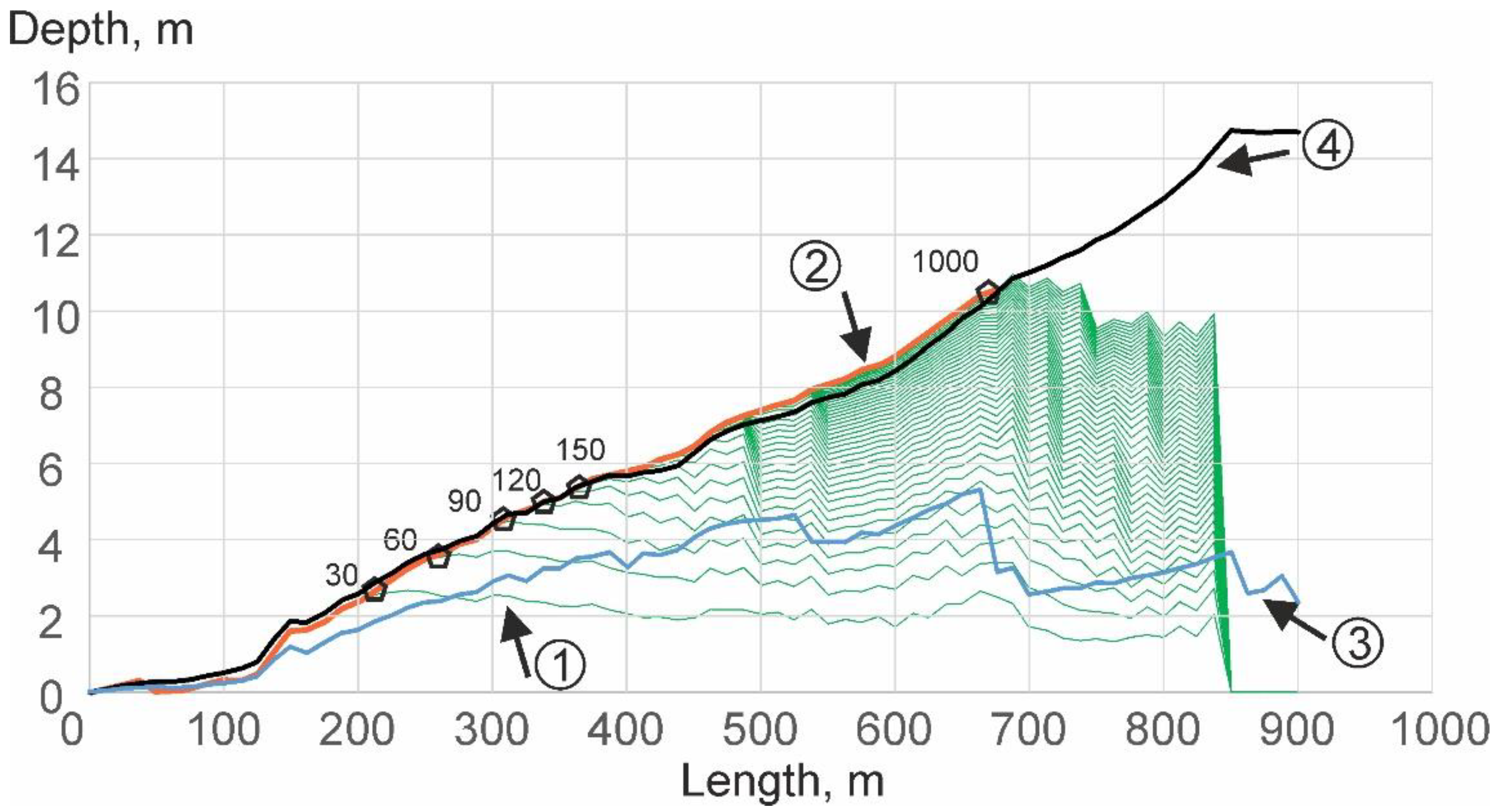
The results of calculations with GULTEM in Figure 5 show a gradual increase of the gully depths and the length of the stable segment of the gully bed through time. At these segments of the gully, its depth does not change anymore. After about 1000 years in calculations, almost the entire gully bed becomes stable, and flow velocities for any discharge become less than critical at all points.
Calculations with STABGUL with the above-described algorithm resulted in the most probable stable longitudinal profile with depths (line 3 in Figure 5), close to the depths from GULTEM after about 120–150 calculation years. This period is close to the period of stabilization of most human-induced gullies on the East European plain [29]. These depths are about 40% less than from GULTEM after 1000 years of calculated erosion (line 2 at Figure 5). The ultimate stable longitudinal profile calculated with STABGUL for the maximum runoff depth (line 4 at Figure 5) fits well with the stable profile after 1000 years from GULTEM. This result shows that the most probable stable longitudinal profile from the STABGUL model can accurately simulate a stable gully after 120–150 years of its lifetime, which can further slowly be transformed to its ultimate stability. It also points out the significance of high discharges on the process of gully erosion.
3.3. The Comparison of the GULTEM and TEP Models
The total erosion potential was calculated in the TEP model along the same flowline and with the same empirical coefficients and hydrological data as gully depth in GULTEM. The similarities and differences in the results (Figure 6) are explained by the similarities and differences in the models’ formulations. Both models operate with the rate of erosion E (Equation (4)), which depends on local slope inclination and specific discharge.
At a given point, the gully depth in GULTEM and erosion potential in TEP are the sum of the product of the erosion rate values and their durations. In GULTEM the products are included to the sum if flow velocity is more than critical, in the TEP model, if runoff depth is more than critical. Therefore, we can expect a correlation of the calculation results. The differences shown are due to the significant simplification in the TEP model of the erosion process. The result of calculations in the TEP model shows the potential of erosion, its position at the catchment, and potential intensity, not gully geometry. In the TEP model, the influence of the altitude of the basis of erosion at the gully mouth and the processes of gully walls slumping are not taken into account. The main difference is the absence in the TEP of the gully longitudinal profile self-forming evolution. Slope inclination in the TEP model is the inclination of the initial slope. Therefore, the correlation between the results of calculation with the two models quickly decreases with time (Figure 7).
3.4. The Comparison of TEP with GER Model
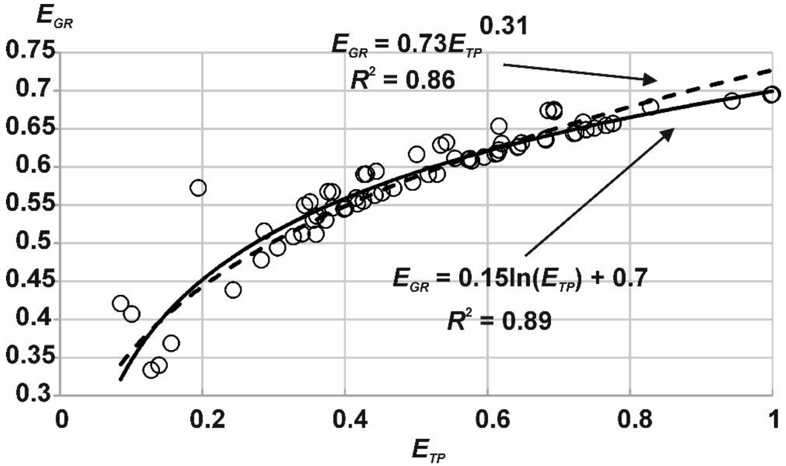
As in previous cases, gully erosion risk was calculated in the GER model along the same flowline and with the same empirical coefficients and hydrological data. There is a close relationship (power-law or logarithmic) between calculation results from the TEP model of total erosion potential ETP and of gully erosion risk EGR in GER (Figure 8). Therefore, the comparison of calculation results from the GER model and GULTEM is more or less the same as in the previous paragraph.
4. Discussion
The problems to be discussed are the availability to possible users of input information, required for calculations with detailed models, and the limitations in simplified models.
The GULTEM is the only model of the four described in this article in which gully evolution can be simulated in “real” time and gully geometry change though time can be adequately simulated. In this model, it is possible to take into account the temporal trends in hydrological information, common in the conditions of global climate change. The temporal and spatial changes in land use, for example, properties of vegetation cover, are also possible to include in the calculations. The large number of input empirical coefficients, morphometric and hydrological data required to run GULTEM is a limitation of the model. The calculations require information for all or particular flowlines in the form of digitized 2D longitudinal profiles of the altitudes of top catchment surface Z (see Figure 2) and of the surfaces Zj of other underlying lithological units along these flowlines. The contributing catchment areas F and coordinates x, y are also collected for the same points. If a digital elevation model (DEM) is available for the catchment, most of this information can be collected using standard tools included in any geographical information system (GIS). The lithological composition of the territory may require investigations in the field.
Parameters and coefficients, used in Equations (4–13), are also better to obtain via measurements at the selected territory, as in [18]. Values of some of these coefficients can be found in special literature. The coefficients in regime Equations (8) and (9) for gullies are discussed in [6,13], the coefficient of thermoerosion in [18], the critical velocity of erosion initiation in [19,30], Manning’s roughness coefficient in [31,32]. The gully walls inclination φ is assumed to equal the angle of repose for a given lithology (see discussion in [33]).
Experimental data on the values of the erosion coefficient kE for cohesive soils, common for gullies, is limited. Experiments and model calibration were provided on soils of the Yamal peninsula [17,18], for silt loams in the gullies of the coast of George Lake in Australia [34], loess soils in the Manawatu River basin and rendzina in the Waimakariri River basin, New Zealand [35] and granodiorite saprolites at the basin of the Mbuluzi River (Swaziland) [36]. The variability of this coefficient is very high. In the direct measurements of sediment budget in the gullies of the Yamal peninsula during the snow thaw and summer rains the value of kE changes from 0.0008 to 0.01 for loams and silt loams with cohesion from 10 to 40 KPa, estimated with a torvane shear tester, and up to 1.3 for loose silt sand. The measurements in Australia showed a similar range of kE: for the loams with cohesion 30–40 KPa 0.0028–0.0034, with cohesion 50–70 kPa—0.0008. The measurements in New Zealand for the loess soil with cohesion 51 kPa showed kE = 0.004–0.005 for soil with organic carbon content 2.4% and kE = 0.021 for the same soil with organic carbon content 0.44%. For rendzina with cohesion 22 kPa and 3.5% content of organic carbon, kE was 2 × 10⁻⁵. Model calibration for the gullies in Swaziland showed kE value 0.006 for sandy saprolites with cohesion 4.5–9 kPa. The listed information was not enough to find the relationship between kE and eroded cohesive soil properties, and the large range of its values does not permit the recommendation of values for calculations on not-investigated objects. The only way to use GULTEM for gully erosion prediction is to calibrate the model on the measurements (see Section 3.1). Usually, such calibration is possible in the framework of detailed projects of land management [36,37].
The complexity in erosion coefficient estimations is the reason to use simpler models for preliminary applications. The models STABGUL, TEP and GER do not require the erosion coefficient. Other parameters and coefficients used in these models, if not estimated in the field measurements, can be found in special literature.
Probability density functions (PDF) of surface runoff values are used in STABGUL and TEP models but for different erosion form lifetimes. The minimum prediction duration in the STABGUL model is about 150 years. Therefore, it is assumed that the time series of hydrological characteristics are stationary. This is not true in the current global climate change, and predictions with STABGUL will not include the trends in the time series of surface runoff. Keeping in mind this limitation, STABGUL is a powerful tool to find the longitudinal profiles, lengths, depths, widths, areas and volumes of the gullies close to the stage of stabilization [16]. This can be useful for the classification of the gullies in the intensively gullied territory to separate stable gullies and those that are still active [38].
The total erosion potential model is based on the modification of the area–slope approach in gully erosion investigations when critical runoff depth is calculated. The TEP model estimates possible gully position in the catchment and erosion intensity. This information can be enough in preliminary projects of land management. The absence of the need for the flowline geometry is the significant simplification: the calculations are performed directly for given points in the catchment, for which slope and contributing area are measured. Calculations of the total erosion potential with the TEP model are more flexible in the conditions of trends in hydrological time series. Much smaller prediction periods are needed in the TEP model (one or a few decades), allowing it to use step functions of PDFs to take into account temporal changes in hydrological statistics. The main limitation of the TEP model is the absence of prediction of the gully geometry.
The GER model requires very limited hydrological data—only maximum daily surface runoff depth for the prediction period. At the same time, the GER model output for a certain catchment contains nearly the same information as total erosion potential from the TEP model, which uses more hydrological data. This similarity is explained by the more or less close relationship between parameters of PDFs of surface runoff values and their maximums. Such relationships are different for different PDFs, as other parameters of PDFs must be taken into account. Therefore, transfer from TEP to GER output will also be different for different hydrological conditions, as unnamed parameters of PDFs are implicitly used in such transfer.
5. Conclusions
The four models described here encompass all now existing approaches to gully erosion prediction. Comparison of the results of calculations for the same gully using these four models makes it possible to choose the model that is most suitable for use in a land management project depending on its objectives and the available information. The set of gully erosion models discussed here can meet the requirements of land management projects with different levels of detail.
Use of the dynamic gully erosion model GULTEM is recommended for calculations of gully geometry transformation in time and space for the most detailed projects of land management. Flowline geometry, soil texture, parameters and coefficients, used in GULTEM, can be obtained via measurements at the selected territory and from DEMs. The calculations take into account the temporal trends in hydrological information, important for conditions of global climate change. The main difficulty in modelling is the estimation of the erosion coefficient, which usually requires calibrating the model.
The input data for the stable gully model STABGUL is the same as for GULTEM, except for the erosion coefficient, which is the most difficult to estimate. Therefore, STABGUL is easier to apply. The STABGUL model is useful for projects where only final gully geometry is required. Only stationary hydrological time series are used in the model.
Possible gully position in the catchment and erosion intensity are estimated with the total erosion potential (TEP) and gully erosion risk (GER) models. The novel type of area–slope approach allows effective use of hydrological information in the form of critical surface runoff for erosion initiation. These models can be useful for preliminary estimates of the possible effects of different land uses.
The presented models, with proper selection of initial data and necessary calibration, can be used for territories with different climates, soils, and land use. They are most effective for areas with possible linear disturbance of the natural vegetation cover, which is typical for the use of land for pastures, for the initial stages of urbanization and the industrial development of new territories.
Funding
This research was funded by Russian State Task 0110—1.13, N 121051100166-4 “Hydrology, morphodynamics, and geoecology of erosion-channel systems”.
Conflicts of Interest
The author declares no conflict of interest.
References
- Poesen, J.; Nachtergaele, J.; Verstraeten, G.; Valentin, C. Gully erosion and environmental change: Importance and research needs. Catena 2003, 50, 91–133. [Google Scholar] [CrossRef]
- Valentin, C.; Poesen, J.; Li, Y. Gully erosion: Impacts, factors and control. Catena 2005, 63, 132–153. [Google Scholar] [CrossRef]
- Bennett, S.; Wells, R. Gully erosion processes, disciplinary fragmentation, and technological innovation. Earth Surf. Process. Landf. 2019, 44, 46–53. [Google Scholar] [CrossRef] [Green Version]
- Sidorchuk, A.Y. Assessing the gully potential of a territory (a case study of central Yamal. Geogr. Nat. Resour. 2020, 41, 178–186. [Google Scholar] [CrossRef]
- Poesen, J.W.A.; Torri, D.; Vanwalleghem, T. Gully erosion: Procedures to adopt when modelling soil erosion in landscapes affected by gullying. In Handbook of Erosion Modelling; Morgan, R.P.C., Nearing, M.A., Eds.; Wiley-Blackwell: Chichester, UK, 2011; pp. 360–386. [Google Scholar] [CrossRef]
- Torri, D.; Poesen, J. A review of topographic threshold conditions for gully head development in different environments. Earth Sci. Rev. 2014, 130, 73–85. [Google Scholar] [CrossRef]
- Schumm, S.A. Geomorphic thresholds: The concept and its applications. Trans. Inst. Brit. Geogr. 1979, NS4, 485–515. [Google Scholar] [CrossRef]
- Patton, P.C.; Schumm, S.A. Gully erosion, north western Colorado: A threshold phenomenon. Geology 1975, 3, 83–90. [Google Scholar] [CrossRef]
- Desmet, P.J.; Poesen, J.; Govers, G.; Vandaele, K. Importance of slope gradient and contributing area for optimal prediction of the initiation and trajectory of ephemeral gullies. Catena 1999, 37, 377–392. [Google Scholar] [CrossRef]
- Vandekerckhove, L.; Poesen, J.; Oostwoudwijdenes, D.; Nachtergaele, J.; Kosmas, C.; Roxo, M.J.; de Figueiredo, T. Thresholds for gully initiation and sedimentation in Mediterranean Europe. Earth Surf. Process. Landf. 2000, 25, 1201–1220. [Google Scholar] [CrossRef]
- Garrett, K.K.; Wohl, E.E. Climate-invariant area–slope relations in channel heads initiated by surface runoff. Earth Surf. Process. Landf. 2017, 42, 1745–1751. [Google Scholar] [CrossRef]
- Woodward, D.E. Method to predict cropland ephemeral gully erosion. Catena 1999, 37, 393–399. [Google Scholar] [CrossRef]
- Nachtergaele, J.; Poesen, J.; Sidorchuk, A.; Torri, D. Prediction of concentrated flow width in ephemeral gully channels. Hydrol. Process. 2002, 16, 1935–1953. [Google Scholar] [CrossRef]
- Kosov, B.F.; Nikolskaya, I.I.; Zorina, Y.F. Experimental research of gullies formation. Exp. Geomorphol. 1978, 3, 113–140. (In Russian) [Google Scholar]
- Zorina, E.F. Quantitative methods of estimating of gully erosion potential. In Soil Erosion and Channel Processes (Eroziya Pochv i Ruslovye Protsessy); Chalov, R.S., Ed.; Moscow Univ. Press: Moscow, Russia, 1979; Volume 7, pp. 81–90. (In Russian) [Google Scholar]
- Sidorchuk, A.; Märker, M.; Moretti, S.; Rodolfi, G. Gully erosion modelling and landscape response in the Mbuluzi River catchment of Swaziland. Catena 2003, 50, 507–525. [Google Scholar] [CrossRef]
- Sidorchuk, A. Dynamic and static models of gully erosion. Catena 1999, 37, 401–414. [Google Scholar] [CrossRef]
- Sidorchuk, A. Gully erosion in the cold environment: Risks and hazards. Adv. Environ. Res. 2015, 44, 139–192. [Google Scholar]
- Sidorchuk, A.; Grigor’ev, V. Soil erosion on the Yamal peninsula (Russian Arctic) due to gas field exploitation. Adv. GeoEcol. 1998, 31, 805–811. [Google Scholar]
- Wolman, M.G.; Miller, J.P. Magnitude and frequency of forces in geomorphic processes. J. Geol. 1960, 68, 54–74. [Google Scholar] [CrossRef] [Green Version]
- Montgomery, D.R.; Dietrich, W.E. Landscape dissection and drainage area-slope thresholds. In Process Models and Theoretical Geomorphology; Kirby, M.J., Ed.; Wiley: New York, NY, USA, 1994; pp. 221–246. [Google Scholar]
- Istanbulluoglu, E.; Tarboton, D.G.; Pack, R.T.; Luce, C. A sediment transport model for incision of gullies on steep topography. Water Resour. Res. 2003, 39, 1103. [Google Scholar] [CrossRef]
- Horton, R.E. Erosional development of streams and their drainage basins: Hydro-physical approach to quantitative morphology. Geol. Soc. Am. Bull. 1945, 56, 275–370. [Google Scholar] [CrossRef] [Green Version]
- Harvey, M.D.; Watson, C.C.; Schumm, S.A. Gully Erosion; Tech. Note 366; U.S. Dept. of the Inter., Bur. of Land Management: Washington, DC, USA, 1985; p. 181.
- Mirtskhulava, Ts.E. Principles of Physics and Mechanics of Channel Erosion (Osnovy Fiziki i Mekhaniki Erozii Rusel); Gidrometeoizdat: Leningrad, Russia, 1988; p. 303. (In Russian) [Google Scholar]
- Sidorchuk, A. The potential of gully erosion on the Yamal peninsula, West Siberia. Sustainability 2020, 12, 260. [Google Scholar] [CrossRef] [Green Version]
- Matveeva, T.; Sidorchuk, A. Modelling of surface runoff on the Yamal peninsula, Russia, using ERA5 reanalysis. Water 2020, 12, 2099. [Google Scholar] [CrossRef]
- Schlesinger, S.; Crosbie, R.E.; Gagne, R.E.; Innis, G.S.; Lalwani, C.S.; Loch, J.; Sylvester, R.J.; Wright, R.D.; Kheir, N.; Bartos, D. Terminology for model credibility. Simulation 1979, 32, 103–104. [Google Scholar]
- Sidorchuk, A.Y.; Golosov, V.N. Erosion and sedimentation on the Russian plain, II: The history of erosion and sedimentation during the period of intensive agriculture. Hydrol. Process. 2003, 17, 3347–3358. [Google Scholar] [CrossRef]
- Van Rijn, L.C. Erodibility of mud-sand bed mixtures. J. Hydraul. Eng.-ASCE 2020, 146, 04019050. [Google Scholar] [CrossRef]
- Chow, V.T. Open-Channel Hydraulics; McGraw-Hill Book Co.: New York, NY, USA, 1959; p. 680. [Google Scholar]
- Engman, E.T. Roughness coefficients for routing surface runoff. J. Irrig. Drain. Eng.-ASCE 1986, 112, 39–53. [Google Scholar] [CrossRef]
- Statham, I. Some limitations to the application of the concept of angle of repose to natural hillslopes. Area 1975, 7, 264–268. [Google Scholar]
- Sidorchuk, A. Dynamic model of gully erosion. In Modelling Soil Erosion by Water; Boardman, J., Favis-Mortlock, D., Eds.; Springer: Berlin/Heidelberg, Germany, 1998; pp. 451–460. [Google Scholar] [CrossRef]
- Sidorchuk, A.; Schmidt, J.; Cooper, G. Variability of shallow overland flow velocity and soil aggregate transport observed with digital videography. Hydrol. Process. 2008, 22, 4035–4048. [Google Scholar] [CrossRef]
- Sidorchuk, A.; Märker, M.; Moretti, S.; Rodolfi, G. Soil erosion modelling in the Mbuluzi River catchment (Swaziland, South Africa). Part I: Modelling the dynamic evolution of gullies. Geogr. Fis. E Din. Quat. 2001, 24, 177–187. [Google Scholar]
- Kayode-Ojo, N.; Ehiorobo, J.O.; Uzoukwu, N. Modelling and prediction of gully initiation in the University of Benin using the GULTEM dynamic model. J. Energy Technol. Policy 2016, 6, 22–32. [Google Scholar]
- Wasson, R.J. Annual and decadal variation of sediment yield in Australia, and some global comparisons. In Variability in Stream Erosion and Sediment Transport; Olive, L.J., Loughran, R.J., Kesby, J.A., Eds.; IAHS Publ. N 224: Wallinford, UK, 1994; pp. 269–279. [Google Scholar]
Figure 1.
The catchment of the large unnamed stable gully with tributary gully P-1 on the Yamal peninsula, Russia (the image of 27 June 2016 from Google Earth). The star on the left part of the figure shows the catchment position.
Figure 1.
The catchment of the large unnamed stable gully with tributary gully P-1 on the Yamal peninsula, Russia (the image of 27 June 2016 from Google Earth). The star on the left part of the figure shows the catchment position.

Figure 2.
The longitudinal profiles of gully P-1, used for model calibration.
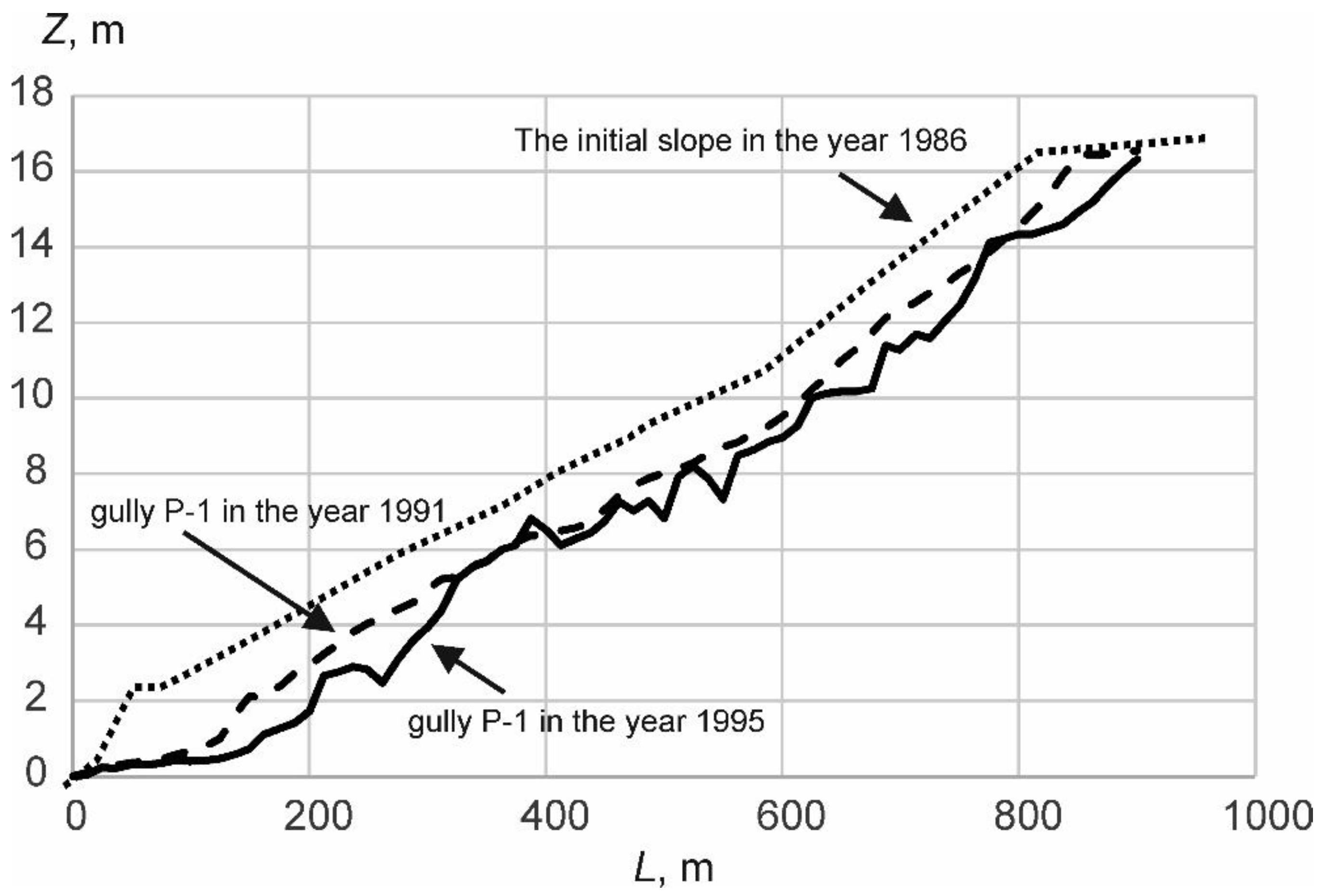
Figure 3.
The result of model calibration.
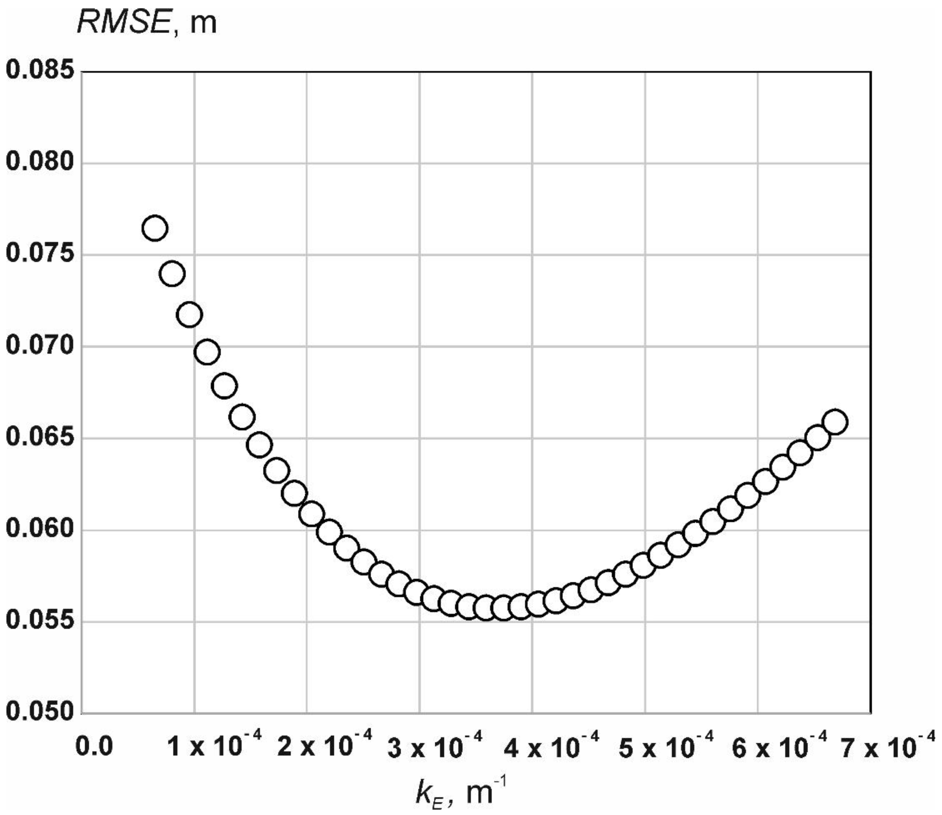
Figure 4.
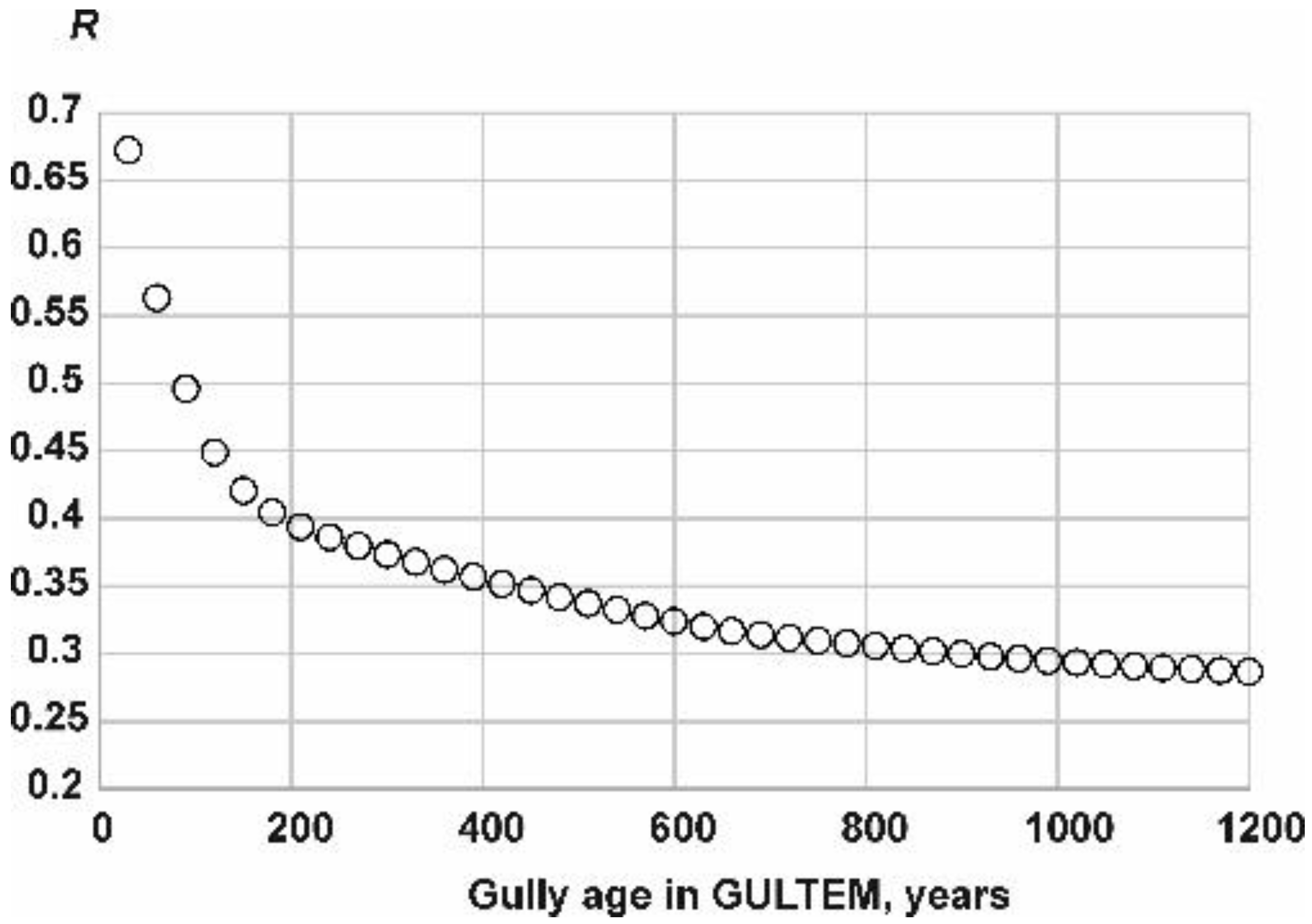
Histogram of daily surface runoff at the gully P-1 catchment.

Figure 5.
The sequence of gully P-1 incision depths calculated with GULTEM for the 1200-year period with 30-year step (green lines 1; pentagrams on some of the lines indicate the age). Red line 2 shows the depths of the gully after 1000 calculation years. Blue line 3 shows the depths of the most probable stable gully, black line 4—the depths of the ultimate stable gully, calculated with the STABGUL model.

Figure 6.
The gully P-1 incision depths for 30-, 150- and 1200-years calculation periods with GULTEM. Black dashed line shows total erosion potential, calculated with the TEP model.
Figure 6.
The gully P-1 incision depths for 30-, 150- and 1200-years calculation periods with GULTEM. Black dashed line shows total erosion potential, calculated with the TEP model.
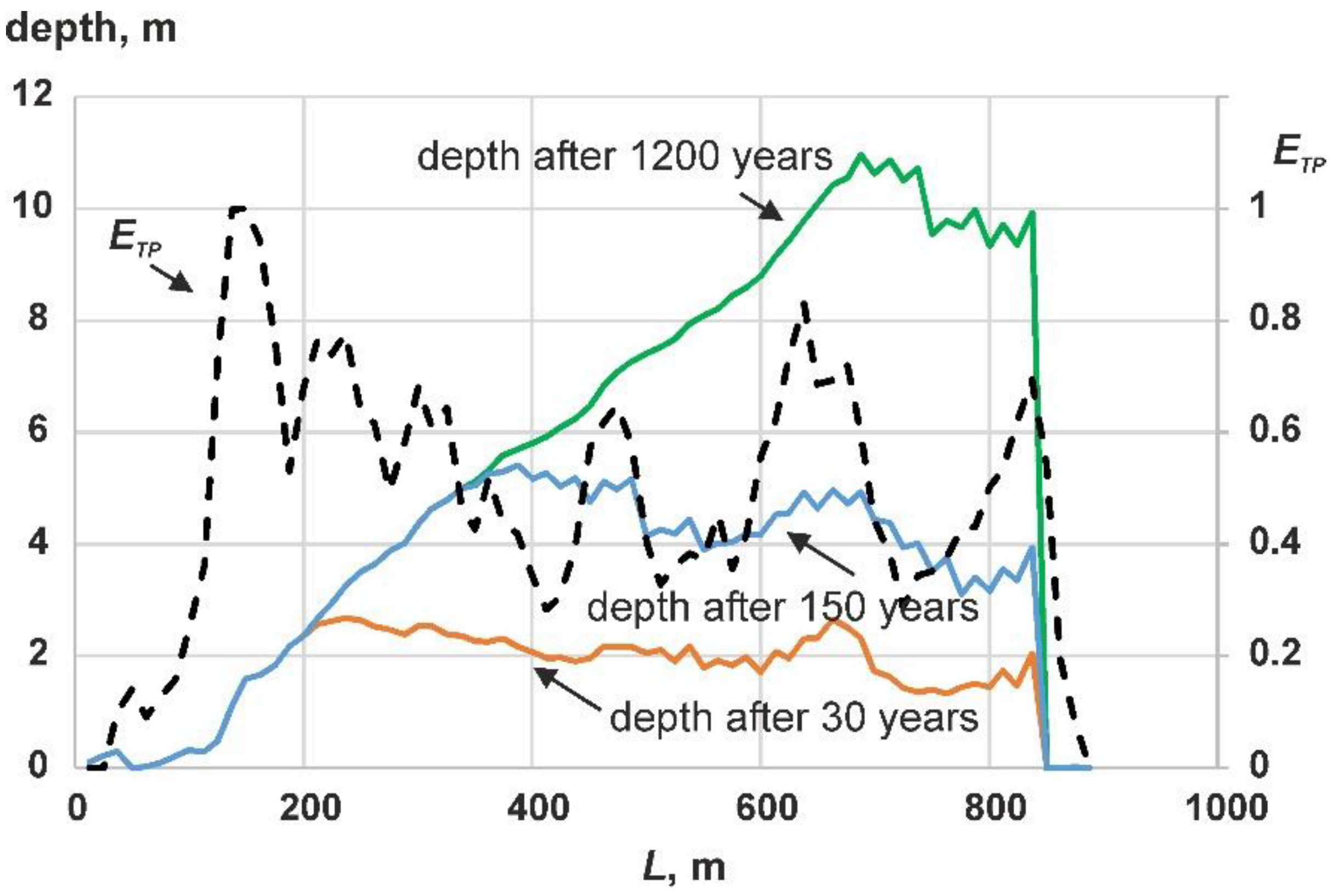
Figure 7.
The decrease of correlation with the increase of prediction time between total erosion potential, calculated with the TEP model, and gully depths, calculated with GULTEM.
Figure 7.
The decrease of correlation with the increase of prediction time between total erosion potential, calculated with the TEP model, and gully depths, calculated with GULTEM.

Figure 8.
The relationship between total erosion potential from TEP and gully erosion risk from GER for the points along the bed profile of gully P-1, shown in Figure 2.
Figure 8.
The relationship between total erosion potential from TEP and gully erosion risk from GER for the points along the bed profile of gully P-1, shown in Figure 2.
Publisher’s Note: MDPI stays neutral with regard to jurisdictional claims in published maps and institutional affiliations. |
© 2021 by the author. Licensee MDPI, Basel, Switzerland. This article is an open access article distributed under the terms and conditions of the Creative Commons Attribution (CC BY) license (https://creativecommons.org/licenses/by/4.0/).
Share and Cite
MDPI and ACS Style
Sidorchuk, A. Models of Gully Erosion by Water. Water 2021, 13, 3293. https://doi.org/10.3390/w13223293
AMA Style
Sidorchuk A. Models of Gully Erosion by Water. Water. 2021; 13(22):3293. https://doi.org/10.3390/w13223293
Chicago/Turabian StyleSidorchuk, Aleksey. 2021. "Models of Gully Erosion by Water" Water 13, no. 22: 3293. https://doi.org/10.3390/w13223293
Note that from the first issue of 2016, this journal uses article numbers instead of page numbers. See further details here.