
Energy Flux Paths in Lakes and Reservoirs


1
Institute for Environmental Sciences, University of Koblenz-Landau, 76829 Landau, Germany
2
Department of Experimental Limnology, Leibniz-Institute of Freshwater Ecology and Inland Fisheries, 12587 Berlin, Germany
3
GFZ German Research Centre for Geosciences, 14473 Potsdam, Germany
4
Institute of Hydrology and Meteorology, Chair of Meteorology, Technische Universität Dresden, 01069 Dresden, Germany
*
Author to whom correspondence should be addressed.
Water 2021, 13(22), 3270; https://doi.org/10.3390/w13223270
Submission received: 6 August 2021
/
Revised: 14 October 2021
/
Accepted: 10 November 2021
/
Published: 18 November 2021
(This article belongs to the Special Issue Physical Processes in Lakes)
Abstract
:Mechanical energy in lakes is present in various types of water motion, including turbulent flows, surface and internal waves. The major source of kinetic energy is wind forcing at the water surface. Although a small portion of the vertical wind energy flux in the atmosphere is transferred to water, it is crucial for physical, biogeochemical and ecological processes in lentic ecosystems. To examine energy fluxes and energy content in surface and internal waves, we analyze extensive datasets of air- and water-side measurements collected at two small water bodies (<10 km2). For the first time we use directly measured atmospheric momentum fluxes. The estimated energy fluxes and content agree well with results reported for larger lakes, suggesting that the energetics governing water motions in enclosed basins is similar, independent of basin size. The largest fraction of wind energy flux is transferred to surface waves and increases strongly nonlinearly for wind speeds exceeding 3 m s−1. The energy content is largest in basin-scale and high-frequency internal waves but shows seasonal variability and varies among aquatic systems. At one of the study sites, energy dissipation rates varied diurnally, suggesting biogenic turbulence, which appears to be a widespread phenomenon in lakes and reservoirs.
Keywords:
energy fluxes; energy content; lakes; reservoirs; internal waves; surface waves; biogenic turbulence1. Introduction
The spatial distribution and temporal dynamics of mechanical energy play vital roles in the physical, biogeochemical and ecological functioning of lentic ecosystems. At the water surface, wind-generated turbulence regulates the vertical distribution of heat that is exchanged with the atmosphere, affects thermal stratification [1] and controls gas exchange with the atmosphere [2], which can be enhanced by surface waves [3]. Vertical turbulent mixing in the surface layer controls the exposure of planktonic organisms to light, therewith regulating primary production and community composition of phytoplankton [4,5,6]. Wind-induced upwelling [7,8], as well as internal waves [9], affect phytoplankton and water quality by transporting nutrients from the stratified hypolimnion to the surface layer. The state of mixing of water bodies can result in the persistence of harmful cyanobacteria in the thermocline throughout summer stratification [10]. At the bottom of lakes and reservoirs, boundary layer turbulence controls the oxygen flux into the sediments [11] and therewith the rate of carbon burial and methane production [12], as well as the internal loading of the lake with nutrients [13].
The major source of mechanical energy in lentic systems is wind, which exerts a shear force at the water surface. However, only a small fraction of the vertical wind energy flux in the atmospheric boundary layer is transferred to water motions (~1.9% according to [14] and ~22% including surface waves in [15]). Water motions are distributed over a wide range of temporal and spatial scales ranging from low to high frequencies of the energy spectrum [15]. Recently, energy transfer from wind to water has been found to be more efficient when the lake is thermally stratified, resulting in an enhancement of mean kinetic energy throughout the water column during seasonal stratification [16,17]. The majority of the wind energy flux is dissipated in the atmospheric and water surface boundary layers. A considerable part of the non-dissipated wind energy (~20%) is fed to the surface wave field [15]. In [18], however, this percentage is lower—1.5–3.5%, although both estimates were derived from the same set of observations conducted in a Swiss lake. Approximately 1% of the energy input is stored in large-scale currents such as basin-scale internal waves [15]. Shear instabilities lead to the degeneration of large-scale internal waves into propagating high-frequency internal waves. They appear at frequencies being some fraction of the maximum buoyancy frequency, which is related to the strength of vertical density stratification [19,20,21]. It has been estimated that about 90% of the energy in the internal waves is dissipated within the bottom boundary layer [14,15].
Current knowledge about the partitioning and distribution of energy fluxes in lakes and reservoirs described above is mainly based on observations from the same lake [16,17], or information compiled from asynchronously conducted measurements in different systems [15]. The generality of current figures, their transferability to water bodies of different size and depth, and their temporal dynamics remain largely unexplored. Moreover, all existing estimates are based on bulk parameterization of wind energy fluxes, as observations lack direct measurements of atmospheric fluxes [14,15,16,17,18]. The role of surface waves in the energy budget appears to be constraint by observations, which are restricted to a single study in a large lake [15,18].
To address these gaps in research, we analyze the most relevant components of energy fluxes and energy content in various types of water motions in response to wind energy fluxes in two small (<10 km2) water bodies. The study sites, a lake and a reservoir, differ in surface area by one order of magnitude, but have comparable water depth (~10 m). Given the difference in surface area and the fact that the reservoir experiences water level variations, we expect the hydrodynamic processes in these two water bodies to be different. The selected lake is considered representative of a large number of small lakes, belonging to the most abundant size class which contributes 54% of the global lake surface area [22,23]. To overcome shortcomings of previous studies, we used direct measurements of momentum fluxes in the atmosphere above the water surface for the estimation of the wind energy flux into the lakes. We investigate the wind speed and fetch dependence on the surface wave characteristics based on measurements covering nearly a complete annual cycle. The predominant modes of basin-scale internal waves and the presence of high-frequency internal waves are identified and examined. The data are used to complement and to re-examine mean energy budgets of small lentic systems, their temporal dynamics, and their variation with water body size.
2. Materials and Methods
2.1. Study Sites and Measurements
Measurements were conducted at a small reservoir (Bautzen Reservoir, surface area: 5.33 km2, volume: 39.2 × 10⁶ m3, maximum depth: 12.2 m) and a small lake (Lake Dagow, surface area: 0.3 km2, volume: 1.2 × 10⁶ m3, maximum depth: 9.5 m)—both situated in Germany. Bautzen Reservoir is a part of the dammed river Spree in southeastern Germany, with a mean water residence time of 164 days [24]. It can be classified as a small storage-type reservoir [25,26] with additional purposes of flood control and leisure activities. Besides, the reservoir is used to regulate the water supply for wetlands and power stations located downstream of the river. The outlet tower located near the dam regulates water discharge through the bottom of the reservoir. Major water withdrawal in summer is associated with a gradual decrease of water level [27]. The reservoir is often not persistently stratified throughout the summer due to a lack of shelter against strong winds and experiences several full mixing events [24,28]. Lake Dagow is a glacial lake in the Lake Stechlin area in northern Germany. It is a small eutrophic lake with a water residence time of 5 years [29]. The lake develops persistent density stratification every year leading to anoxic conditions in its hypolimnion [29]. Lake Dagow was impacted by wastewater, duck and carp farming in the 1960–1970s, with restoration activities in the 1980s.
At both water bodies, a similar set of instruments was installed for a period resolving the seasonal dynamics of stratification and mixing in Bautzen Reservoir (3 April until 3 December in 2018) and the transition from stratified to mixed conditions during the autumn overturn in Lake Dagow (11 September until 25 November in 2017). Meteorological measurements, including radiation fluxes and eddy covariance (EC) measurements of vertical momentum fluxes, were conducted from floating platforms (Points A and E, Figure 1). The platform was 3 × 3 m in size in Bautzen Reservoir and about 2.5 × 5 m in size in (Lake Dagow). Both platforms were attached with steel chains (Bautzen Reservoir) or guy wires (Lake Dagow) to four concrete anchors at the bottom. Vertical profiles of flow velocity in the water column, including turbulent velocity fluctuations, were measured by acoustic Doppler current profilers (ADCP), which were mounted downward-facing at the platforms (see Table 1). In Bautzen reservoir, the profiling range of the platform-mounted ADCP did not cover the entire water column and an additional ADCP was deployed at the bottom at ~10 m distance from the platform. The bottom-mounted instrument did not resolve turbulent velocity fluctuations and provided mean flow velocity profiles only. In Lake Dagow, there were three sequential ADCP deployments with time gaps in between. The ADCP was installed at the bottom during the second and third deployments. Thermistor chains were deployed at the platform in Bautzen Reservoir and in the middle of Lake Dagow to observe vertical temperature stratification in water. Wave recorders (high-frequency pressure loggers) were placed near the shore at both locations and an additional wave recorder was installed at the platform in Bautzen Reservoir. The measurement campaign lasted from 3 April until 3 December in 2018 in Bautzen Reservoir and from 11 September until 25 November in 2017 in Lake Dagow.
Detailed information about instrumentation and resolution is provided in Table 1. As described in the following sections, the collected data were analyzed to characterize energy fluxes from wind to water and the energy content in different types of water motion. Meteorological data were screened based on plausibility limits, logged information about maintenance work at the measurement station, and by detection of errors and outliers. ADCP velocity data were filtered using a threshold for signal correlation (>70 (-)) and were despiked following [30,31]. All final parameters were estimated with a temporal resolution of 30 min.
2.2. Energy Content
2.2.1. Internal Waves
Standing, basin-scale internal waves (internal seiches) are characterized by oscillations of the vertical density structure that appears due to wind forcing acting on the stratified lake. Waves are typically present in the form of one or several energetic modes depending on the density layer structure [32]. In our study, we identified the major modes of internal waves using the “Internal Wave Analyzer” software (IWA) [33] and selected wave “events” when visual evidence of their presence was observed. Visual evidence appeared in vertical displacements of isotherms and as a pronounced peak in the power spectral density estimated for variations in isothermal depths and for the selected velocity components. Similarly, events were identified for propagating (high frequency) internal waves, which were mainly present in the spectra of the vertical velocity component and displacement of isotherms during the stratified season. The high-frequency limit of the wave band in spectra is limited by the maximum buoyancy frequency Nmax (Hz) [19,34]:
where g (m s−2) is gravitational acceleration, ρw (kg m−3) is water density, ρw0 (kg m−3) is the mean water density, z (m) is the height above the bottom with positive direction upwards. The conversion from temperature to density was done based on the freshwater equation of state following [35].
The energy content in a linear internal wave field is equally partitioned into potential energy and kinetic energy [36]. An appropriate approach for estimation of the energy is calculation of the locally available potential energy (APE (J m−3)) from temporal variations of water density observed at a single mooring location [37,38]:
where ζ (m) is the vertical displacement of a fluid particle and z′ is the integration variable. We estimated potential energy at 30 min resolution (or 1 min for high-frequency internal waves) by using different time intervals for estimating the mean (background) density stratification. As a rule of thumb, we considered 10 periods of the observed wave, either the basin-scale or high-frequency internal wave, for calculating mean density profiles. In addition, for basin-scale internal waves we estimated kinetic energy from the spectra of the three velocity components within the frequency band corresponding to the range of the wave periods provided by IWA. For high-frequency internal waves a fixed frequency range from 1 × 10⁻³ to 6.1 × 10⁻³ Hz was selected.
For comparison with surface energy fluxes, we integrated the volumetric energy content over depth. Both integrated potential and kinetic energies (as well as dissipation rate described in Section 2.4), were normalized by depth-dependent surface area, i.e., for a given quantity X, integration over the water column was computed as:
where Asurf is the surface area of the water body, H is the water depth, A is the depth-dependent cross-sectional area.
2.2.2. Surface Waves
Significant wave height Hsig (m) and energy content in surface waves Ewave (J m−2) were calculated from pressure fluctuations measured by the wave recorders. The calculation was carried out following standard procedures based on linear wave theory [40] by using the “Ruskin” software provided by the manufacturer [41]. The calculations take into account the attenuation of wave-induced pressure fluctuations at the sampling depth of the sensor. Significant wave height is defined as the average height of the highest one third of the waves during each sampling interval. Mean wave energy was calculated from the variance of water surface elevation. Note that for Bautzen Reservoir we used only those wave measurements that corresponded to the acceptable wind directions (195–355°) to avoid the possible sheltering effect of the measurement platform (the sensor was deployed at the south-western corner).
2.2.3. Schmidt Stability
The Schmidt stability Sc (J m−2) describes the integrated potential energy in vertical density stratification of the entire basin. It is equivalent to the work required for vertical mixing, i.e., the energy required to move the vertical coordinate of the center of mass of all water in the basin to the corresponding center of volume zv:
where V is the volume of the basin.
2.3. Energy Fluxes
2.3.1. Wind Energy Flux and Rate of Working
The vertical energy flux at a standard height of 10 m above the water surface P10 (W m−2) is equivalent to the vertical shear stress multiplied by the horizontal wind velocity [42]:
where (kg m−1 s−1) is the shear stress, (m s−1) is the atmospheric friction velocity and ρa (kg m−3) is air density. In our analysis, we estimated from measurements of turbulent velocity fluctuations in the atmospheric boundary layer using the eddy-covariance (EC) method [43]. The mean wind speed measured at a height of 1.8 m (Bautzen Reservoir) and 1.97 m (Lake Dagow) above the water surface was corrected to a standard height of 10 m ( (m s−1)) by considering atmospheric stability [44,45]. We calculated the fraction of the wind energy that is transferred to the water as the total rate of working RW (W m−2) following [16]:
where the wind () and flow velocity (u,v) components were rotated along the wind direction averaged over 12 h since the shape of two water bodies does not have any preferred elongated direction. The drag coefficient CDN10 was first determined as (-) and then corrected to its neutral counterpart , where κ = 0.4 (-) is the von Kármán constant, L is the Monin-Obukhov length scale and ψ are the stability functions described in [44]. Note that, we used the first acceptable measurement of flow velocity below the surface: for Bautzen Reservoir, it corresponds to ~1 m depth, for Lake Dagow ~0.6 m (first deployment), ~1.3 m (second and third deployment).
2.3.2. Surface Wave Energy Flux
The horizontal wave energy flux per unit length of the wave crest of surface waves (Pwave (W m−1)) was calculated as the product of the wave energy and the wave group velocity. The group velocity is a function of wave period, which we assign to the period corresponding to the maximum in the wave spectrum. The estimation of the wave energy flux proceeds in the same way as in [46]. To compare Pwave with the wind energy flux P10, we considered the ratio Pwave/(P10 × F) 100 (%), where F (m) is the wind fetch at the wave measurement location. The wind fetch is interpolated from distances obtained from the map corresponding to the standard grid of wind direction. Note that, as in Section 2.2.2, we disregarded data with unacceptable wind directions for Bautzen Reservoir.
2.3.3. Surface Heat Flux and Buoyancy Flux
The net surface energy flux in form of heat and radiation Hnet (W m−2) is expressed as the sum of net shortwave radiation QSW, longwave radiation QLW, and latent and sensible heat fluxes HL, HS (W m−2). Latent and sensible heat fluxes were calculated following the standard EC methodology using the “Eddy Pro Version 6.2.1” software (LI-COR, Inc., Lincoln, NE, USA).
The surface buoyancy flux JBO (W m−2) was calculated as:
where α (K−1) is the temperature-dependent thermal expansion coefficient of water and cp (J kg-1 K−1) is the specific heat capacity of water.
2.3.4. Energy Flux to Basin-Scale Internal Waves
For the estimation of the fraction of the wind energy input attributed to basin-scale internal waves, we manually selected isolated episodes with solitary wind event and corresponding enhancement of the available potential energy in internal waves. This fraction (%) was calculated as a ratio of APE averaged over one cycle of the wave right after the wind event to the wind energy flux integrated over the time for the respective wind event.
2.4. Dissipation Rates
Dissipation rates of turbulent kinetic energy ε (W kg−1) were estimated following two methods: inertial subrange fitting (ISF) [47] and second-order structure function (SF) [48]. Both methods have been widely applied and validated for obtaining dissipation rates from velocity data measured by ADCP [49,50,51,52]. Under the assumption of isotropic turbulence, the theoretical power spectrum of turbulent velocity fluctuations S (m3 s−2 rad−1) is expressed as:
where αK = 1.5 (-) is the universal Kolmogorov constant, k (rad m−1) is the spatial wavenumber and C1 (-) is the isotropy constant, which depends on the direction of the velocity component 18/55 ≤ C1 ≤ 4/3 × 18/55. We used a constant value of C1 = 18/55 as we used beam-averaged velocity spectra from the ADCP, which measures along-beam velocity fluctuations without directional information [53]. Power spectra estimated from measurements were fitted to Eq. 10 to estimate the dissipation rates. The upper wavenumber limit for the fit was found as a breakpoint where the power spectral density became smaller than the level of noise. The noise level was determined as the logarithmically averaged high-frequency end of the spectra at frequencies higher than 0.2 Hz. To find the lower frequency limit for inertial subrange fitting, we used the optimization procedure described in [54]. We used three criteria for quality assurance for calculated dissipation rates: validity of Taylor’s frozen turbulence hypothesis, coefficient of determination of the fit (for both—see [47]) and the length of observed inertial subrange (set to a minimum of 10/8 of decade). The application of these quality criteria led to significant reduction in dissipation rate estimated using ISF (~70% of the data were removed).
Due to the presence of surface waves in velocity spectra, we could not apply ISF for the entire period of measurements. We manually selected velocity spectra where no sur-face wave peak was observed. For periods when no inertial subrange could be observed in the spectra, we applied the SF method, which can be corrected for the case when surface waves are present [55]:
where D(z,r) (m2 s−2) is the mean squared velocity difference at two locations separated by the distance r (m), C2 = 2.1 (-) is a constant, C3 (-) is a coefficient describing wave orbital motion and Nm (m2 s−2) is the measurement noise. C3, C2 ε2/3 and Nm were determined using least square fits of measured along-beam velocity fluctuations to Equation (11). We used fixed numbers of ADCP bins for the fitting. First, we applied the procedure with 5 bins (for the purpose of the calculations the number of bins should be odd). We noticed that noise could be negative in cases when the theoretical structure function was not long enough to reach its “plateau”. Therefore, we used the procedure with seven bins and replaced the values of dissipation rates from the previous step for cases when the noise was negative. We disregarded fits, if either Nm, C2 ε2/3, the difference between the first point of the structure function and the noise, or the difference between the second and first point of the structure function were negative. The application of these criteria led to ~51% and ~30% reduction of the dissipation rate estimates for Bautzen Reservoir and Lake Dagow, respectively.
The dissipation rates obtained from both ISF and SF methods agreed reasonably well (see Figure S1, Supplementary Material). However, the scatter at low dissipation rates increases towards the bottom and the structure function estimates were a factor of 2 to 3 lower than the ISF estimates for dissipation rates exceeding 1 × 10⁻⁸ W kg−1. The final dissipation rates combined both estimates using ISF and SF techniques considering the ISF calculations as default value and gap-filling with estimates from SF.
The ISF method could be applied for the full depth range of the velocity measurements. Application of the SF method results in dissipation profiles that lack several bins at the beginning and at the end of the profiling range due to the calculation procedure but could be applied in the presence of surface waves. Thus, we combined the advantages of both methods. However, this procedure was applied and validated for Bautzen Reservoir data, while for Lake Dagow only the SF method was used. That was because there were only few periods during which the velocity spectra were not affected by surface waves during the first deployment and application of the ISF method was not possible for most of the time.
Logarithmic velocity profiles in the bottom boundary layer (BBL) were not resolved by our ADCP measurements at both locations due to the limited profiling range. Visual observation of the flow velocity profiles revealed that the BBL extended up to ~2 m distance above the bottom. Dissipation rates in the BBL were calculated using the flow velocity (m s−1) at the measurement depth (ADCP bin) closest to the bottom using the law of the wall [56]:
where (m s−1) is the bottom friction velocity. Following [56], the bottom drag coefficient was corrected for the distance from the bottom at which the flow speed was measured, using a standard value of 1.5 × 10⁻³ at 1 m height. Resulting dissipation rate profiles were integrated over depth as in Equation (3) and multiplied by density of the water ρw to obtain areal estimates of depth-integrated dissipation rates (in W m−2).
3. Results
3.1. Overview of the Measurements
The measurements include both stratified and mixed conditions throughout 243 days in Bautzen Reservoir and the transition from seasonal summer stratification to mixed conditions during the autumn overturn (76 days) in Lake Dagow (Figure 2). In Bautzen Reservoir, the temperature stratification during summer was occasionally disrupted by winds exceeding 7 m s−1. These mixing events are consistent with observations at this reservoir reported in previous studies [24,28,57]. The maximum temperature at the water surface was 29.2 °C (4 August) in Bautzen Reservoir and 18 °C (11 September) in Lake Dagow. The maximum temperature difference between surface and bottom was 15.2 °C (10 June) and 8 °C (12 September) in Bautzen Reservoir and Lake Dagow, respectively. In Lake Dagow, the thermocline was located close to the bottom and the thickness of the hypolimnion was only ~0.7 m. Average Schmidt stability was 4.3 and 41.8 J m−2 and maximum values were 21 J m−2 (17 September) and 178 J m−2 (01 June) in Lake Dagow and Bautzen Reservoir, respectively. The heat and buoyancy fluxes varied between −155 and 1113 W m−2 (−5.1 × 10⁻⁴ and 4.2 × 10⁻³ W m−2) in Bautzen Reservoir and between −130 and 763 W m−2 (−2.6 × 10⁻⁴ and 3.1 × 10⁻³ W m−2) in Lake Dagow (buoyancy flux in parenthesis, Table S1, Figure S8, Supplementary Material).
Wind forcing in both systems was of the same order of magnitude: the wind speed at 10 m height was 3.0 ± 1.9 and 2.7 ± 1.7 m s−1 (here and further, ± denotes standard deviation) with maximum values of 13.7 and 10.1 m s−1 in Bautzen Reservoir and Lake Dagow, respectively. West-northwestern (280–300°) and south-western (220–240°) wind directions were predominant for Bautzen Reservoir and Lake Dagow, respectively. The water level continuously declined throughout the study period from 11.2 m to 6.8 m at the platform location in Bautzen Reservoir, while in Lake Dagow it remained constant (~8.3 m at the ADCP location). Water discharge at the inflow and at the outlet tower varied between 0.6 and 3.9 m3 s−1, with mean values of 1.2 and 1.9 m3 s−1, respectively (Figure S2, Supplementary Material). In both water bodies, flow velocities were relatively small for most of the time (~0.01–0.02 m s−1). The maximum flow speed was 0.1 m s−1 in Bautzen Reservoir and 0.07 m s−1 in Lake Dagow. The mean significant wave height Hsig was (3.9 ± 9.6) × 10−3 m and (1.9 ± 2.7) × 10−2 m at shore sampling locations (Point B in Bautzen Reservoir, Point G in Lake Dagow, see Figure 1) and (7.4 ± 9.9) × 10−2 m at the platform in Bautzen Reservoir. The maximum value of significant wave height was 0.1 and 0.2 m for the shore sampling locations in Lake Dagow and Bautzen Reservoir, respectively, and 0.5 m at the platform in Bautzen Reservoir.
3.2. Wind Energy Flux and Rate of Working
The ratio of the wind energy flux at 10 m height (P10) to the rate of working associated with shear stress in the surface layer of the water column (RW) provides an estimate of the efficiency of the energy transfer from wind to water. We analyzed the ratio separately for mixed and for stratified conditions, but we did not find significant differences between both conditions (Figure 3). We used a fixed, although arbitrary, threshold for Schmidt stability (Sc = 5 J m−2) to distinguish between mixed and stratified conditions. Distributions of the ratio of RW to P10 for periods when the Schmidt stability was smaller or larger than 5 J m−2 were in close agreement (Figure S3, Supplementary Material). The median values of the ratio were 1.8 × 10⁻³ and 1.6 × 10⁻³ in Bautzen Reservoir, and 1.7 × 10⁻³ and 0.7 × 10⁻³ in Lake Dagow for non-stratified and stratified conditions, respectively. We applied linear regressions of RW as a function of P10 considering P10 less than 2 W m−2, as most of the data belonged to this interval. Different values of the threshold in Schmidt stability to distinguish stratified and mixed conditions did not result in significant changes in slopes. However, we noticed that the slope of the regression was sensitive to the inclusion of few high-magnitude values. The slope coefficient for all data, which describes the efficiency of energy transfer is equal to (1.3 ± 0.1) × 10−3 and (2.61 ± 0.05) × 10−3 (± here denotes standard error for the slope) for Bautzen Reservoir and Lake Dagow, respectively. Data from Bautzen Reservoir were additionally filtered based on the same wind directions as for surface waves (Section 2.2.2) to avoid potential sheltering by the measurement platform. These values were comparable to the mean efficiency of 1.3 × 10⁻³ estimated under mixed conditions in a lake by [16].
3.3. Surface Waves
We examined the relationship between significant wave height and wind speed at 10 m height (Figure 4a) and compared our wave measurements with the only—to the best of our knowledge—other existing dataset of significant wave height in relation to wind speed in a lake. These data were measured in a large lake in Switzerland over a two-week period [18]. Although the significant wave height reached higher values in [18] (~0.5 m) than in our measurements (~0.3 m, at the platform location in Bautzen Reservoir), the wind-speed dependence is remarkably consistent in both datasets. Wave heights were relatively small (<1 × 10⁻² m) with weak dependence on wind speed for winds below ~3 m s−1, while wave heights strongly increased for wind speeds exceeding 3–4 m s−1. Significant wave heights measured at the shore locations were generally smaller in amplitude and showed a weaker increase with increasing wind compared to open-water measurements (Figure 4a). This could be related to the interference with waves reflected from the shore and shallow water depth at the sampling locations.
We applied an empirical approach for the prediction of significant wave height based on the wave frequency, wind speed and fetch length, which was originally derived from measurements in the North Sea but is also commonly used in lake models (the Joint Sea Wave Project or JONSWAP, [58]). The parameterization overestimated the significant wave height up to wind speeds of approximately 4 m s−1 and underestimated wave heights for higher wind speeds (see blue lines, Figure 4a). This supported the earlier finding of [18]; however, their “breakpoint” was at around 6 m s−1 and the JONSWAP predictions agreed well with the measurements at higher wind speed. The authors of [18] note that the possible reasons for underestimation at low wind speeds could either be insufficient sensor accuracy to resolve the small amplitude of waves, or a failure to compute the wind fetch correctly as the variability in wind direction at low wind speeds is very high. The wind fetch indeed varied considerably due to the variations in wind direction; however, smoothing of the calculated fetch prior to applying the wave model did not significantly reduce the predicted values at low wind speeds. The JONSWAP model overestimated the significant wave height for both measurements at shore locations.
Energy content in surface waves varied between 1.3 × 10⁻⁴ and 9.1 × 10² J m−2 with a log-averaged value of 0.3 J m−2 for the measurements at the platform in Bautzen Reservoir. In Lake Dagow, it varied between 1.6 × 10⁻⁴ and 1.1 × 101 J m−2 with a log-averaged value of 1.5 × 10⁻³ J m−2. Wave energy measured at the shore in Bautzen Reservoir (1.3 × 10⁻⁴–2.1 × 101 J m−2 with log-averaged value 2 × 10⁻² J m−2) was comparable in magnitude to the shore measurements in Lake Dagow. Wave energy showed strong dependence on the wind speed exceeding 3 m s−1 with a power-law exponent of ~8–9 (Figure S4, Supplementary Material).
The median values of the fraction of the wind energy input attributed to the surface waves (see Section 2.3.2) varied between 0.05% and 0.4% between sampling locations (Figure 4b). Mean values varied between 0.5% and 4%. The fraction strongly increased for wind speeds exceeding 3 m s−1.
3.4. Internal Waves
Basin-scale and high-frequency internal waves were observed in both water bodies. The prevailing mode of basin-scale waves was the second vertical mode/first horizontal mode (V2H1), with a period of approximately 8–9 and 12 h and maximum amplitude of 1–2 m and 0.5–1 m in Bautzen Reservoir and Dagow Lake, respectively (Figure 5). Note, that we also observed waves with a period of approximately 21 h in both water bodies; however, they occurred only once during a short period of time. Although a clear periodic structure of the waves was present below the thermocline (Figure 5a), close to the surface it was often masked by wind-driven flow and mixed layer dynamics. Unlike basin-scale internal waves, high-frequency internal waves occurred not only during summer stratification but also during autumn and spring mixing. The period of the major wave peak in the power spectra of velocity and isothermal depths varied throughout the measurements from 5–6 min during the stratified season up to 15–20 min during mixing in spring and autumn. High-frequency internal waves appeared in the frequency range 0.02–0.2 N, which was lower than values reported for larger lakes (0.1–0.7 N) [59,60,61,62].
Energy content in basin-scale and high-frequency internal waves is comprised of available potential energy (APE) and kinetic energy (see Section 2.2.1). We analyzed its seasonal dynamics, using the long-term measurement from Bautzen Reservoir (Figure 6a). During the deepening of the upper mixed layer in spring, the average APE during internal wave events (for the definition of “event” see Section 2.2.1) had a maximum of 6.7 J m−2, while it remained nearly constant below 1 J m−2 during most of the time. Its average value for 13 analyzed internal wave events was 1.2 ± 1.0 J m−2. Note that the periods of the internal waves in the two last events (October and November, see Figure 6a) were not supported by the predictions of the Internal Wave Analyzer; however, we visually observed internal waves as a peak in the velocity spectrum. The average APE in high-frequency internal waves evaluated for 210 events reached its maximum value of 0.45 J m-2 in summer during the strongest stratification (end of June–beginning of September). The average value over the entire measurement period was 0.06 ± 0.05 J m−2.
The mean kinetic energy during the selected basin-scale internal wave events was on average a factor of four smaller than the APE. This inconsistency with linear wave theory can be explained by the location of measurements relative to the lake center. In standing waves, the kinetic energy is higher near the center, whereas the potential energy is higher along the edges. However, for high-frequency internal waves, the average kinetic energy for all selected events was 0.05 J m−2, which was comparable to the APE (note that the difference between them is greater during April to August, probably because velocity measurements cover only the upper part of the water column). In Lake Dagow, we identified only one event with basin-scale internal wave activity and the corresponding APE of 0.05 J m−2 was two orders of magnitude smaller than in Bautzen Reservoir because the thermocline was close to the bottom. Following [14], we used the double value of APE as a measure of the total energy in internal waves.
The fraction of the wind energy flux, which is transferred to basin-scale internal waves was estimated based on nine selected episodes with solitary wind events in Bautzen Reservoir and three in Lake Dagow (see Section 2.3.4). One example is presented in Figure 6b, which demonstrates how waves are energized by a wind event. The average percentage of wave energy and integrated wind energy flux amounted up to 0.1% with an average value of 0.04 ± 0.03%. In Lake Dagow, the energy flux to internal waves was 0.002%, which is one order of magnitude lower than the average value in Bautzen.
3.5. Dissipation Rate in Surface and Bottom Boundary Layers
The log-averaged dissipation rates of turbulent kinetic energy were of the same order of magnitude (~10−8 W kg−1) in Bautzen Reservoir and Lake Dagow (Figure 7). They tended to increase towards the water surface, while remaining nearly constant in the middle of the water column. Estimates of dissipation rate in the bottom boundary layer (Equation (12)) were on average one (Bautzen Reservoir) and two (Lake Dagow) orders of magnitude smaller than dissipation rates in the interior and the surface layer.
In Lake Dagow, the BBL approach may not be appropriate as there was a possible influence of biogenic activity, which may contribute additional turbulence or interfere with the analysis method. We observed a strong diurnal variation in the dissipation rate (primarily during the first deployment; see Figures S5 and S8, Supplementary Material). However, in contrast to similar observations [17,63], we observed high acoustic backscatter during the night (see Figure S5b, Supplementary Material) and an increase in dissipation rates and vertical velocity occurred during the day (Figure S5b, Supplementary Material). It is important to note that high dissipation rates were present in the entire water column and not just close to the bottom where elevated acoustic backscatter was observed. We also observed a “trace” of high dissipation rates starting from midnight when migrating zooplankton species begin to swim towards the bottom. We suggest that strong acoustic backscatter during the night and high dissipation rate and vertical flow velocity patterns during the day (see average profiles for days and nights in Figure S5, Supplementary Material) are related to diurnal migrations of different types of organisms. The pronounced diurnal pattern of dissipation rates and backscatter strength became less obvious in the second and third ADCP deployments suggesting the reduction of the number of species in autumn.
Depth-integrated dissipation rates were typically three orders of magnitude smaller than the wind energy flux (Figures S6–S8, Supplementary Material). The dissipation rates integrated over the BBL were on average two orders of magnitude lower than the dissipation rates integrated over the interior and surface boundary layer (Figure S7, Supplementary Material). The share of the wind energy input that was dissipated in turbulence increased with wind speed. In Bautzen Reservoir, highest values of depth-integrated dissipation rates were comparable in magnitude to the corresponding wind energy flux (Figure S6a, Supplementary Material). We observed a strong relationship between the integrated dissipation rate and wind energy flux with a power-law exponent of ~2.6 for wind speeds exceeding ~3 m s−1 in Bautzen Reservoir (Figure S7). We did not find this relationship in the data from Lake Dagow, where the wind energy flux reached comparable magnitude, but integrated dissipation rates remained below the high values observed in Bautzen Reservoir. However, rare events with high integrated energy dissipation rates did not contribute to mean conditions. The average ratio of total integrated dissipation rate and wind energy flux was 0.23% and 0.5% for Bautzen Reservoir and Lake Dagow, respectively. Similarly, the mean values of depth-integrated dissipation rates were a factor of two lower in Bautzen (1.7 × 10⁻⁵ W m−2) compared to Lake Dagow (3.4 × 10⁻⁵ W m−2).
4. Discussion
4.1. Overall Energy Budget
Based on simultaneous measurements of energy fluxes in the atmospheric boundary layer and along the water column in two small water bodies, we compiled energy budgets in terms of energy fluxes and energy content in different types of water motions (Figure 8, Table S1, Supplementary Material). Despite having different origin and differing in size by one order of magnitude, the reservoir and the lake feature similar hydrodynamic processes and energy flux paths. Most of the vertical energy flux at 10 m above the water surface is dissipated in the atmospheric boundary layer (~95% of the wind energy flux) and is not transferred to the water body. The remaining fraction is distributed into various types of water motions.
The largest fraction of wind energy flux (0.5–4%) is transferred to surface waves. Energy dissipation in turbulent flows accounted for 0.2–0.5% of the wind energy flux, while one order of magnitude less energy is transferred to basin-scale internal waves (0.002–0.04%). The energy content is largest in basin-scale internal waves in Bautzen Reservoir, where it is about one order of magnitude higher than the energy content in surface waves, as well as in high-frequency internal waves. Lake Dagow, the energy content is of comparable magnitude in all type of waves. Generally, the energy content in water motions is small compared to the potential energy in thermal stratification (Schmidt stability), which differed on average by one order of magnitude between both water bodies. The average wind energy flux in the atmosphere exceeded the average buoyancy flux by two orders of magnitude in both water bodies (Figure 8).
Some important components of the energy budget are lacking, including turbulent kinetic energy and kinetic energy in large-scale water motions such as water currents (except for waves). As discussed in the following sections, our results revealed a number of important findings related to specific energy flux paths, as well as to the potential generalization of the derived energy budget to other lakes and reservoirs.
4.2. Energy Transfer Efficiency
The estimated efficiency of energy transfer from wind to water derived from wind energy flux and rate of working in the surface layer was in close agreement for both water bodies, despite their difference in surface area. The estimated rate of wind working can be considered as an independent estimate of the energy transfer from wind to water. It can be obtained by summing up the relevant components of the energy budget (Table S1). Taking the mean shear and flow velocity at the water surface into account, the RW should be equal to the sum of all energy fluxes, except for surface waves, which are not resolved in the estimation of the RW. The sum of the components was dominated by depth-integrated energy dissipation rates (0.23–0.5% of P10), which were slightly higher but of the same order of magnitude as RW (0.14–0.27% of P10). Generally, this agreement supports the magnitudes of the energy fluxes compiled in Figure 8.
In contrast to earlier studies on Lake Windermere [16,17], there was no evidence of intensification of the energy transfer from the wind to the water during the stratified season compared to the period of lake mixing. The efficiency of wind energy input for both water bodies was found to be within the values reported for non-stratified conditions [14]. However, we did find a strong, non-linear increase of the efficiency with increasing wind speed in Bautzen reservoir. This fact was in line with our finding that estimates of a mean transfer efficiency are sensitive to including the few largest observations. We observed a close agreement between the mean transfer efficiencies estimated in the present study for two water bodies differing by an order of magnitude in surface area and those reported in [14] for Lake Windermere South Basin, which is slightly larger in size than Bautzen Reservoir but considerably deeper. This agreement suggests that the values represent a robust order-of-magnitude estimate for aquatic systems of small to medium size.
4.3. Surface and Internal Waves
The fraction of the wind energy flux attributed to surface waves was up to 4% on average and within the range reported by [13,16] based on measurements in a large (214 km2) lake in Switzerland. However, this fraction strongly increased with the wind speed exceeding 3 m s−1 and depended on the sampling location. We demonstrated that the JONSWAP model for the estimation of the significant wave height may not be an appropriate approach for estimating significant wave heights in smaller lakes and reservoirs as it significantly overestimated wave height at low wind speed. At high wind speed, we found an extremely strong increase of wave energy with a power-law coefficient of ~8–9 with wave height exceeding the JONSWAP predictions. More wave observations in different lakes and reservoirs and further detailed investigation of the relationship between the wave characteristics and wind speed are needed to improve predictions of wave height and wave energy fluxes in lakes and reservoirs.
The energy content in basin-scale internal waves was on average lower than values reported for a larger and deeper alpine lake in [14] (0.1–2.4 J m−2 versus 22 ± 3 J m−2) and slightly higher than the values in [15] (10−2–1 J m−2). We assume that this difference can be related to the strength of stratification and lake depth. The alpine lakes studied in [14] and [15] showed persistent and large-amplitude internal seiching, which occurred rather sporadically and with smaller amplitudes in Bautzen and Dagow. In addition, the energy content in basin-scale internal waves varied with season and was on average five-fold higher in spring than for the remaining sampling period in Bautzen Reservoir. This can be explained by the deepening of the thermocline and the way of calculation of the energy content with the thermocline depth being the upper limit for vertical integration. Also, lake bathymetry can affect the seasonal variation of the internal waves [64]. The energy flux to the basin-scale internal waves can be up to 0.1% of the wind energy flux but is on average two orders of magnitude smaller than that reported for the alpine lake (0.04% versus 1% in [13]). Energy content in high-frequency internal waves was on average one order of magnitude smaller than in basin-scale internal waves (Bautzen Reservoir) and comparable with basin-scale internal waves in Lake Dagow. During the stratified season, high-frequency waves can contain on average twice as much energy than during the remaining period.
4.4. Energy Dissipation Rates
Average energy dissipation rates were of the same order of magnitude in both water bodies (~5 × 10⁻⁹ W kg−1). More energy was dissipated with increasing wind energy flux. Although in Bautzen Reservoir at high wind speeds almost all of the wind energy flux was dissipated, this was not observed at Lake Dagow, which may be related to the smaller size of the lake and the sheltering effect of the surrounding forest. On average, a similar percentage of the wind energy flux was dissipated in both water bodies. However, the dissipation rates estimated for the bottom boundary layer were on average one (Bautzen Reservoir) and two (Lake Dagow) orders of magnitude smaller than those calculated for the remaining water column. This can potentially be explained by the fact that flow velocities were generally very low, and the boundary layer may not be observed within the ADCP profiling range, making an underestimation of the dissipation rates possible.
The other possible explanation for such a difference in the dissipation rates in Lake Dagow is biogenic activity. We observed high acoustic backscatter in the upper part of the water column during the night and at larger depth during daytime, suggesting diurnal vertical migration of zooplankton [65]. Recent studies found higher dissipation rates at depths of high acoustic backscatter [17,63], suggesting a contribution of migrating organisms to energy dissipation. In contrast to these observations, we observed enhanced dissipation rates at depths and at times of low acoustic backscatter. The difference in dissipation rates between day and night can be up to two orders of magnitude. As pointed out in [65], the acoustic backscatter strength is affected by both the abundance and the acoustic properties of the scatterers and can be dominated by organisms containing gas bubbles. Other organisms, such as small fish, may follow opposing migration patterns, which remain hidden in the volume backscatter strengths [66]. Aggregations of small swimming fish with densities of 5–8 m−3 have been shown to enhance dissipation rates by one order of magnitude [67]. The role of biogenic turbulence in marine in inland waters has been widely discussed and analyzed in the past decade (see reviews in [68,69]). The main conclusion was that although small swimmers may generate additional flow and energy dissipation, they are unlikely to contribute to vertical mixing. Small swimmers generate flow disturbances at the scale of some multiple body length [70]. The dissipation rate estimates from ADCP are limited by the relatively large size of the sampling volume (bin size) and are theoretically based on turbulent energy transfer from large to small scales. These limitations may challenge the measurement of energy dissipation rates with ADCP in the presence of small swimmers. The increasing reporting of diurnal patterns in energy dissipation rates in relation to acoustic backscatter in recent studies calls for careful validation of these estimates using alternative methods for estimating dissipation rates, such as microstructure profiling and particle image velocimetry.
4.5. Study Limitations
In addition to the methodological limitations and uncertainties mentioned above, a number of limitations of our analysis should be noted. We made single-point measurements, and internal waves were not spatially resolved. Additional measurements along the direction of the internal wave may allow to estimate the potential and kinetic energy in wave motions more precisely. To assess the possible effect of lake bathymetry and morphology on internal wave structure and seasonal variability, spatially resolved flow measurements can be combined with numerical models in future studies.
In addition, we did not analyze the potential impact of the water level variation in Bautzen Reservoir on the energy fluxes. Reduction of the water level in a medium-sized reservoir shortens the stratification period [71,72]. This would affect the energy content in the basin-scale internal waves, at least in the way we calculated it. Possible interference of the internal waves with the lakebed may cause more turbulence in the bottom boundary layer. However, it is difficult to distinguish between the effect of water level variation and the seasonal change in the lake thermal structure without additional modeling.
Furthermore, we assumed that the wind speed is horizontally homogeneous over the lake for all sampling locations. This may not be applicable and additional, spatially resolving meteorological measurements should be included in future studies. The uncertainties in the estimation of dissipation rates could be related to the selection of the constants (in inertial subrange fitting and structure function methods). For example, [52,73] showed that these constants depend on the distance from the boundary and the use of the “canonical” constants may lead to significant errors. In addition, it remains unclear how flow and energy dissipation generated by small swimming organisms affect measurements and bulk parameterizations of energy dissipation rates.
5. Conclusions
For the first time, we related observations of energy content and fluxes in different types of water motion to simultaneously measured energy fluxes in the atmospheric boundary layer. Although the two studied water bodies were expected to be governed by contrasting hydrodynamic processes and conditions, we did not find any significant differences in energy fluxes. The observed and estimated energy fluxes and energy content agree well with results reported for larger water bodies, suggesting that the energetics governing water motions in enclosed basins is similar, independent of basin size.
Only a small fraction (<5%) of the vertical wind energy flux in the atmosphere is transferred to water motions. By disregarding surface waves, the efficiency of energy transfer does not differ strongly between various water bodies of different sizes. The transfer efficiency increases with increasing wind energy flux, but we could not observe significant differences of the energy efficiency under stratified and mixed conditions, as it has been reported for a deeper lake.
Our measurements highlight the importance of surface waves, which receive the largest share of the wind energy flux into the water and have mostly been neglected in previous studies. The wave energy flux increases strongly nonlinearly with increasing wind speed for wind speed exceeding 3 m s−1. Existing parametrizations of wave height as a function of wind speed and fetch length fail to reproduce observed wave amplitudes in small water bodies.
The largest energy content was observed in basin-scale internal waves, which was found to be within the range reported for larger lakes. However, the energy fluxes and energy content in internal waves seem to vary strongly among lakes having different size and depth. Internal waves appear to be more important in mean energy budgets in larger and deeper lakes.
Dissipation rates of turbulent kinetic energy show similar structure and dynamics and are of comparable magnitude in water bodies of different size. Similar to surface waves, depth-integrated dissipation rates increase strongly nonlinearly if the wind energy flux exceeds a threshold value, which corresponds to a wind speed of 3 m s−1. We observed a pronounced diurnal pattern in dissipation rates at one of our study sites, which is most likely related to vertically migrating organisms. The reliability of commonly applied measurement and analysis procedures for estimating energy dissipation rates in the presence of swimming organisms needs to be confirmed in future studies.
Supplementary Materials
The following are available online at https://www.mdpi.com/article/10.3390/w13223270/s1, Figure S1: Dissipation rate estimated using structure function method (SF) versus dissipation rate calculated using inertial subrange fitting method (ISF) at ~1.5 m depth for measurements in Bautzen Reservoir (gray dots). Figure S2: Discharge of the inflow (red line) and outflow (at the outlet tower) of Bautzen reservoir. The data was provided by the the Landestalsperren-Verwaltung Sachsen (LTV). Figure S3: Probability distribution of the ratio of rate of working (RW) to wind energy flux (P10) selected for two cases: Schmidt stability (Sc) < 5 J m−2 (area shown in gray, corresponding to non-stratified conditions) and Sc ≥ 5 J m−2 (area shown in red, corresponding to stratified conditions) for (a) Bautzen Reservoir. The median values are 1.8 × 10⁻³ and 1.6 × 10⁻³, the average values (±standard deviation) are (2 ± 4)·10−3 and (0.6 ± 21.6)·10−2, for non-stratified and stratified conditions, respectively. (b) Lake Dagow. Figure S4: Surface wave energy versus wind speed at 10 m height at the platform location in Bautzen Reservoir (gray dots). Wave energy shows strong dependence on wind speed exceeding 2–3 m s−1. The black line shows bin-average data, the red line represents a power-law relationship with an exponent of nine. The latter was obtained from a linear regression of log-transformed data. Figure S5: (a) Dissipation rates of turbulent kinetic energy averaged over night and over daytime during the first ADCP deployment in Lake Dagow. (b) Acoustic backscatter strength recorded by the ADCP (upper panel), vertical flow velocity (middle panel), dissipation rate (lower panel). Figure S6: Depth-integrated dissipation rate (including surface and bottom boundary layers and interior of the water bodies) versus the vertical wind energy flux above the water surface in (a) Bautzen Reservoir; (b) Lake Dagow. Figure S7: Dissipation rate integrated over the bottom boundary layer (the thickness of 2 m, light gray dots) and over the rest of the water column where the ADCP measurements are available (dark gray dots) using data from (a) Bautzen Reservoir; (b) Lake Dagow. The gray solid line represents a 1:1 relationship. Figure S8: Temporal dynamics of wind energy flux (black line, upper panel), dissipation rates integrated over the water depth (red dots, upper panel) and buoyancy flux (lower panel) for data measured in (a) Bautzen Reservoir; (b) Lake Dagow. Note the pronounced diurnal pattern in integrated energy dissipation rates in Lake Dagow during the first ADCP deployment (cf. Figure S4). Table S1: Energy content and energy fluxes.
Author Contributions
Conceptualization by A.L., S.G. and U.S.; methodology by U.S., P.C., T.S. and A.L.; formal analysis by S.G. and A.L.; writing—original draft preparation by S.G., U.S., P.C., T.S, A.L; data curation by U.S., S.G. and T.S.; visualization by S.G; supervision by A.L. All authors have read and agreed to the published version of the manuscript.
Funding
S.G. and A.L. were supported by the German Research Foundation (Deutsche Forschungsgemeinschaft, DFG) under the grant LO1150/12-1. Eddy Covariance measurements at Lake Dagow (T.S.) used infrastructure of the Terrestrial Environmental Observatories Network (TERENO) and were supported by the Helmholtz Young Investigators Grant (VH-NG-821) of the Helmholtz Association of German Research Centers. U. S. was participated in project “Greenhouse Gas Emissions from Reservoirs: Mechanisms and Quantification (TREibhausGAsemissionen von TAsperren—TREGATA)” which was funded by the DFG and was listed under the project number 288267759.
Institutional Review Board Statement
Not applicable.
Informed Consent Statement
Not applicable.
Data Availability Statement
The water-side measurements from Bautzen Reservoir and Lake Dagow are openly available in Zenodo at 10.5281/zenodo.5159088. The meteorological data from Lake Dagow presented in this study is openly available in FLUXNET at https://doi.org/10.18140/FLX/1669633 (accessed 20 August 2021) [74]. The meteorological and temperature data from Bautzen Reservoir are available on request from U. S. The data are not publicly available due to ongoing research. The data of discharge at the outlet tower (Bautzen Reservoir) is property of the Landestalsperren-Verwaltung Sachsen (LTV).
Acknowledgments
We strongly appreciate the help and support with instrumentation and maintenance from Christoph Bors, Gonzalo Santaolalla, Jens Nejstgaard, Tim Walles, Christian Wille, Philipp Keller, Matthias Koschorreck, Christian Bernhofer, Heiko Prasse, Uwe Eichelmann, Markus Hehn, and Martin Wieprecht. We thank Christian Wille for providing materials for the study.
Conflicts of Interest
The authors declare no conflict of interest.
References
- Imberger, J. Flux paths in a stratified lake: A review. In Physical Processes in Lakes and Oceans; American Geophysical Union: District of Columbia, WA, USA, 1998; pp. 1–17. [Google Scholar]
- Jähne, B.; Haußecker, H. Air-Water Gas Exchange. Annu. Rev. Fluid Mech. 1998, 30, 443–468. [Google Scholar] [CrossRef]
- Perolo, P.; Fernández Castro, B.; Escoffier, N.; Lambert, T.; Bouffard, D.; Perga, M.-E. Accounting for Surface Waves Improves Gas Flux Estimation at High Wind Speed in a Large Lake. In Dynamics of the Earth System; Interactions: Franklin, MA, USA, 2021. [Google Scholar]
- MacIntyre, S. Vertical Mixing in a Shallow, Eutrophic Lake: Possible Consequences for the Light Climate of Phytoplankton. Limnol. Oceanogr. 1993, 38, 798–817. [Google Scholar] [CrossRef]
- Huisman, J.; Sharples, J.; Stroom, J.M.; Visser, P.M.; Kardinaal, W.E.A.; Verspagen, J.M.H.; Sommeijer, B. Changes in Turbulent Mixing Shift Competition for Light between Phytoplankton Species. Ecology 2004, 85, 2960–2970. [Google Scholar] [CrossRef] [Green Version]
- Peeters, F.; Straile, D.; Lorke, A.; Ollinger, D. Turbulent Mixing and Phytoplankton Spring Bloom Development in a Deep Lake. Limnol. Oceanogr. 2007, 52, 286–298. [Google Scholar] [CrossRef]
- Corman, J.R.; McIntyre, P.B.; Kuboja, B.; Mbemba, W.; Fink, D.; Wheeler, C.W.; Gans, C.; Michel, E.; Flecker, A.S. Upwelling Couples Chemical and Biological Dynamics across the Littoral and Pelagic Zones of Lake Tanganyika, East Africa. Limnol. Oceanogr. 2010, 55, 214–224. [Google Scholar] [CrossRef] [Green Version]
- Bocaniov, S.A.; Schiff, S.L.; Smith, R.E.H. Plankton Metabolism and Physical Forcing in a Productive Embayment of a Large Oligotrophic Lake: Insights from Stable Oxygen Isotopes: Plankton Metabolism and Physical Forcing. Freshw. Biol. 2012, 57, 481–496. [Google Scholar] [CrossRef]
- MacIntyre, S.; Jellison, R. Nutrient Fluxes from Upwelling and Enhanced Turbulence at the Top of the Pycnocline in Mono Lake, California. Hydrobiologia 2001, 466, 13–29. [Google Scholar] [CrossRef]
- Sepúlveda Steiner, O. Mixing Processes and Their Ecological Implications: From Vertical to Lateral Variability in Stratified Lakes; EPFL: Lausanne, Switzerland, 2020. [Google Scholar]
- Lorke, A.; Müller, B.; Maerki, M.; Wüest, A. Breathing Sediments: The Control of Diffusive Transport across the Sediment-Water Interface by Periodic Boundary-Layer Turbulence. Limnol. Oceanogr. 2003, 48, 2077–2085. [Google Scholar] [CrossRef]
- Sobek, S.; Durisch-Kaiser, E.; Zurbrügg, R.; Wongfun, N.; Wessels, M.; Pasche, N.; Wehrli, B. Organic Carbon Burial Efficiency in Lake Sediments Controlled by Oxygen Exposure Time and Sediment Source. Limnol. Oceanogr. 2009, 54, 2243–2254. [Google Scholar] [CrossRef] [Green Version]
- Søndergaard, M.; Jensen, J.P.; Jeppesen, E. Role of Sediment and Internal Loading of Phosphorus in Shallow Lakes. Hydrobiologia 2003, 506–509, 135–145. [Google Scholar] [CrossRef]
- Wüest, A.; Piepke, G.; Van Senden, D.C. Turbulent Kinetic Energy Balance as a Tool for Estimating Vertical Diffusivity in Wind-Forced Stratified Waters. Limnol. Oceanogr. 2000, 45, 1388–1400. [Google Scholar] [CrossRef]
- Imboden, D.M. The Motion of Lake Waters. In The Lakes Handbook, Volume 1; O’Sullivan, P.E., Reynolds, C.S., Eds.; Blackwell Science Ltd.: Malden, MA, USA, 2003; pp. 115–152. ISBN 978-0-470-99927-1. [Google Scholar]
- Woolway, R.I.; Simpson, J.H. Energy Input and Dissipation in a Temperate Lake during the Spring Transition. Ocean Dyn. 2017, 67, 959–971. [Google Scholar] [CrossRef]
- Simpson, J.H.; Woolway, R.I.; Scannell, B.; Austin, M.J.; Powell, B.; Maberly, S.C. The Annual Cycle of Energy Input, Modal Excitation and Physical Plus Biogenic Turbulent Dissipation in a Temperate Lake. Water Res. 2021, 57, e2020WR029441. [Google Scholar] [CrossRef]
- Simon, A. Turbulent Mixing in the Surface Boundary Layer of Lakes. Ph.D. Thesis, Swiss Federal Institute of Technology, Zürich, Switzerland, 1997. [Google Scholar]
- Heyna, B.; Groen, P. On Short-Period Internal Gravity Waves. Physica 1958, 24, 383–389. [Google Scholar] [CrossRef]
- Boegman, L.; Ivey, G.N.; Imberger, J. The Energetics of Large-Scale Internal Wave Degeneration in Lakes. J. Fluid Mech. 2005, 531, 159–180. [Google Scholar] [CrossRef] [Green Version]
- Preusse, M.; Peeters, F.; Lorke, A. Internal Waves and the Generation of Turbulence in the Thermocline of a Large Lake. Limnol. Oceanogr. 2010, 55, 2353–2365. [Google Scholar] [CrossRef] [Green Version]
- Downing, J.A.; Prairie, Y.T.; Cole, J.J.; Duarte, C.M.; Tranvik, L.J.; Striegl, R.G.; McDowell, W.H.; Kortelainen, P.; Caraco, N.F.; Melack, J.M.; et al. The Global Abundance and Size Distribution of Lakes, Ponds, and Impoundments. Limnol. Oceanogr. 2006, 51, 2388–2397. [Google Scholar] [CrossRef] [Green Version]
- Choulga, M.; Kourzeneva, E.; Zakharova, E.; Doganovsky, A. Estimation of the Mean Depth of Boreal Lakes for Use in Numerical Weather Prediction and Climate Modelling. Tellus A Dyn. Meteorol. Oceanogr. 2014, 66, 21295. [Google Scholar] [CrossRef] [Green Version]
- Rinke, K.; Hübner, I.; Petzoldt, T.; Rolinski, S.; König-Rinke, M.; Post, J.; Lorke, A.; Benndorf, J. How Internal Waves Influence the Vertical Distribution of Zooplankton. Freshw. Biol. 2007, 52, 137–144. [Google Scholar] [CrossRef] [Green Version]
- Poff, N.L.; Hart, D.D. How Dams Vary and Why It Matters for the Emerging Science of Dam Removal. BioScience 2002, 52, 659. [Google Scholar] [CrossRef] [Green Version]
- Tundisi, J.G. Limnology; CRC Press: Boca Raton, FL, USA, 2017; ISBN 978-1-138-07204-6. [Google Scholar]
- Kerimoglu, O.; Rinke, K. Stratification Dynamics in a Shallow Reservoir under Different Hydro-Meteorological Scenarios and Operational Strategies. Water Resour. Res. 2013, 49, 7518–7527. [Google Scholar] [CrossRef]
- Wagner, A.H.; Janssen, M.; Kahl, U.; Mehner, T.; Benndorf, J. Initiation of the Midsummer Decline of Daphnia as Related to Predation, Non-Consumptive Mortality and Recruitment: A Balance. Arch. Hydrobiol. 2004, 160, 1–23. [Google Scholar] [CrossRef]
- Casper, S.J. Lake Stechlin: A Temperate Oligotrophic Lake; Springer: Berlin/Heidelberg, Germany, 2012; Volume 58. [Google Scholar]
- Goring, D.G.; Nikora, V.I. Despiking Acoustic Doppler Velocimeter Data. J. Hydraul. Eng. 2002, 128, 117–126. [Google Scholar] [CrossRef] [Green Version]
- Wahl, T.L. Discussion of “Despiking Acoustic Doppler Velocimeter Data” by Derek G. Goring and Vladimir I. Nikora. J. Hydraul. Eng. 2003, 129, 484–487. [Google Scholar] [CrossRef] [Green Version]
- Münnich, M.; Wüest, A.; Imboden, D.M. Observations of the Second Vertical Mode of the Internal Seiche in an Alpine Lake. Limnol. Oceanogr. 1992, 37, 1705–1719. [Google Scholar] [CrossRef]
- De Carvalho Bueno, R.; Bleninger, T.; Lorke, A. Internal Wave Analyzer for Thermally Stratified Lakes. Environ. Model. Softw. 2021, 136, 104950. [Google Scholar] [CrossRef]
- Antenucci, J.P.; Imberger, J. On Internal Waves near the High-Frequency Limit in an Enclosed Basin. J. Geophys. Res. 2001, 106, 22465–22474. [Google Scholar] [CrossRef]
- Chen, C.-T.A.; Millero, F.J. Thermodynamic Properties for Natural Waters Covering Only the Limnological Range. Limnol. Oceanogr. 1986, 31, 657–662. [Google Scholar] [CrossRef]
- Kundu, P.K.; Cohen, I.M.; Dowling, D.R. Gravity Waves. In Fluid Mechanics; Elsevier: Amsterdam, The Netherlands, 2012; pp. 253–307. ISBN 978-0-12-382100-3. [Google Scholar]
- Holliday, D.; Mcintyre, M.E. On Potential Energy Density in an Incompressible, Stratified Fluid. J. Fluid Mech. 1981, 107, 221. [Google Scholar] [CrossRef]
- Kang, D.; Fringer, O. On the Calculation of Available Potential Energy in Internal Wave Fields. J. Phys. Oceanogr. 2010, 40, 2539–2545. [Google Scholar] [CrossRef]
- Read, J.S.; Hamilton, D.P.; Jones, I.D.; Muraoka, K.; Winslow, L.A.; Kroiss, R.; Wu, C.H.; Gaiser, E. Derivation of Lake Mixing and Stratification Indices from High-Resolution Lake Buoy Data. Environ. Model. Softw. 2011, 26, 1325–1336. [Google Scholar] [CrossRef]
- RBR Ltd. Wave Parameters. Available online: https://docs.rbr-global.com/support/ruskin/ruskin-features/waves/wave-parameters (accessed on 25 July 2021).
- Ruskin Software. Available online: https://rbr-global.com/products/software (accessed on 25 July 2021).
- Imboden, D.M.; Wüest, A. Mixing Mechanisms in Lakes. In Physics and Chemistry of Lakes; Lerman, A., Imboden, D.M., Gat, J.R., Eds.; Springer: Berlin/Heidelberg, Germany, 1995; pp. 83–138. ISBN 978-3-642-85134-6. [Google Scholar]
- Foken, T.; Nappo, C.J. Micrometeorology; Springer: Berlin/Heidelberg, Germany, 2008; ISBN 978-3-540-74665-2. [Google Scholar]
- Paulson, C.A. The Mathematical Representation of Wind Speed and Temperature Profiles in the Unstable Atmospheric Surface Layer. J. Appl. Meteorol. Climatol. 1970, 9, 857–861. [Google Scholar] [CrossRef]
- Large, W.G.; Pond, S. Open Ocean Momentum Flux Measurements in Moderate to Strong Winds. J. Phys. Oceanogr. 1981, 11, 324–336. [Google Scholar] [CrossRef] [Green Version]
- Hofmann, H.; Lorke, A.; Peeters, F. The Relative Importance of Wind and Ship Waves in the Littoral Zone of a Large Lake. Limnol. Oceanogr. 2008, 53, 368–380. [Google Scholar] [CrossRef]
- Bluteau, C.E.; Jones, N.L.; Ivey, G.N. Estimating Turbulent Kinetic Energy Dissipation Using the Inertial Subrange Method in Environmental Flows: TKE Dissipation in Environmental Flows. Limnol. Oceanogr. Methods 2011, 9, 302–321. [Google Scholar] [CrossRef]
- Wiles, P.J.; Rippeth, T.P.; Simpson, J.H.; Hendricks, P.J. A Novel Technique for Measuring the Rate of Turbulent Dissipation in the Marine Environment. Geophys. Res. Lett. 2006, 33, L21608. [Google Scholar] [CrossRef]
- Guerra, M.; Thomson, J. Turbulence Measurements from Five-Beam Acoustic Doppler Current Profilers. J. Atmos. Ocean. Technol. 2017, 34, 1267–1284. [Google Scholar] [CrossRef]
- McMillan, J.M.; Hay, A.E. Spectral and Structure Function Estimates of Turbulence Dissipation Rates in a High-Flow Tidal Channel Using Broadband ADCPs. J. Atmos. Ocean. Technol. 2017, 34, 5–20. [Google Scholar] [CrossRef]
- Lorke, A. Boundary Mixing in the Thermocline of a Large Lake. J. Geophys. Res. 2007, 112, C09019. [Google Scholar] [CrossRef] [Green Version]
- Jabbari, A.; Rouhi, A.; Boegman, L. Evaluation of the Structure Function Method to Compute Turbulent Dissipation within Boundary Layers Using Numerical Simulations. J. Geophys. Res. Oceans 2016, 121, 5888–5897. [Google Scholar] [CrossRef]
- Lorke, A.; Wüest, A. Application of Coherent ADCP for Turbulence Measurements in the Bottom Boundary Layer. J. Atmos. Ocean. Technol. 2005, 22, 1821–1828. [Google Scholar] [CrossRef] [Green Version]
- Guseva, S.; Aurela, M.; Cortes, A.; Kivi, R.; Lotsari, E.S.; Macintyre, S.; Mammarella, I.; Ojala, A.; Stepanenko, V.M.; Uotila, P.; et al. Variable Physical Drivers of Near-Surface Turbulence in a Regulated River. Water Resour. Res. 2021, 57. [Google Scholar] [CrossRef]
- Scannell, B.D.; Rippeth, T.P.; Simpson, J.H.; Polton, J.A.; Hopkins, J.E. Correcting Surface Wave Bias in Structure Function Estimates of Turbulent Kinetic Energy Dissipation Rate. J. Atmos. Ocean. Technol. 2017, 34, 2257–2273. [Google Scholar] [CrossRef]
- Lorke, A.; MacIntyre, S. The Benthic Boundary Layer (in Rivers, Lakes, and Reservoirs). In Encyclopedia of Inland Waters; Elsevier: Amsterdam, The Netherlands, 2009; pp. 505–514. ISBN 978-0-12-370626-3. [Google Scholar]
- Benndorf, J.; Kranich, J.; Mehner, T.; Wagner, A. Temperature Impact on the Midsummer Decline of Daphnia galeata: An Analysis of Long-Term Data from the Biomanipulated Bautzen Reservoir (Germany): Temperature Impact on Midsummer Decline. Freshw. Biol. 2001, 46, 199–211. [Google Scholar] [CrossRef]
- Hasselmann, K.F.; Barnett, T.; Bouws, E.; Carlson, H.; Cartwright, D.; Enke, K.; Ewing, J.; Gienapp, H.; Hasselmann, D.; Meerburg, A.; et al. Measurements of Wind-Wave Growth and Swell Decay during the Joint North Sea Wave Project (JONSWAP). Ergänzungsheft zur Dtsch. Hydrogr. Z. Reihe A 1973, 12, 1–95. Available online: http://hdl.handle.net/21.11116/0000-0007-DD3C-E (accessed on 14 October 2021).
- Mortimer, C.H.; McNaught, D.C.; Stewart, K.M. Short Internal Waves near Their High-Frequency Limit in Central Lake Michigan. In Proceedings of the 11th Annual Conference on Great Lakes Research, Milwaukee, WI, USA, 18–20 April 1968; pp. 454–469. [Google Scholar]
- Thorpe, S.A. High-Frequency Internal Waves in Lake Geneva. Phil. Trans. R. Soc. Lond. A 1996, 354, 237–257. [Google Scholar] [CrossRef]
- Stevens, C.L. Internal Waves in a Small Reservoir. J. Geophys. Res. 1999, 104, 15777–15788. [Google Scholar] [CrossRef]
- Gímez-Giraldo, A.; Imberger, J.; Antenucci, J.P.; Yeates, P.S. Wind-Shear-Generated High-Frequency Internal Waves as Precursors to Mixing in a Stratified Lake. Limnol. Oceanogr. 2008, 53, 354–367. [Google Scholar] [CrossRef]
- Ishikawa, M.; Bleninger, T.; Lorke, A. Hydrodynamics and Mixing Mechanisms in a Subtropical Reservoir. Inland Waters 2021, 11, 286–301. [Google Scholar] [CrossRef]
- Fricker, P.D.; Nepf, H.M. Bathymetry, Stratification, and Internal Seiche Structure. J. Geophys. Res. 2000, 105, 14237–14251. [Google Scholar] [CrossRef]
- Lorke, A.; McGinnis, D.F.; Spaak, P.; Wuest, A. Acoustic Observations of Zooplankton in Lakes Using a Doppler Current Profiler. Freshw. Biol. 2004, 49, 1280–1292. [Google Scholar] [CrossRef]
- Lorke, A.; Weber, A.; Hofmann, H.; Peeters, F. Opposing Diel Migration of Fish and Zooplankton in the Littoral Zone of a Large Lake. Hydrobiologia 2008, 600, 139–146. [Google Scholar] [CrossRef] [Green Version]
- Lorke, A.; Probst, W.N. In Situ Measurements of Turbulence in Fish Shoals. Limnol. Oceanogr. 2010, 55, 354–364. [Google Scholar] [CrossRef]
- Kunze, E. Biologically Generated Mixing in the Ocean. Annu. Rev. Mar. Sci. 2019, 11, 215–226. [Google Scholar] [CrossRef]
- Simoncelli, S.; Thackeray, S.J.; Wain, D.J. Can Small Zooplankton Mix Lakes? Limnol. Oceanogr. 2017, 2, 167–176. [Google Scholar] [CrossRef]
- Wickramarathna, L.N.; Noss, C.; Lorke, A. Hydrodynamic Trails Produced by Daphnia: Size and Energetics. PLoS ONE 2014, 9, e92383. [Google Scholar] [CrossRef] [PubMed]
- Nowlin, W.H.; Davies, J.-M.; Nordin, R.N.; Mazumder, A. Effects of Water Level Fluctuation and Short-Term Climate Variation on Thermal and Stratification Regimes of a British Columbia Reservoir and Lake. Lake Reserv. Manag. 2004, 20, 91–109. [Google Scholar] [CrossRef]
- Bonnet, M.-P.; Poulin, M.; Devaux, J. Numerical Modeling of Thermal Stratification in a Lake Reservoir. Methodology and Case Study. Aquat. Sci. 2000, 62, 105. [Google Scholar] [CrossRef]
- Jabbari, A.; Boegman, L.; Valipour, R.; Wain, D.; Bouffard, D. Dissipation of Turbulent Kinetic Energy in the Oscillating Bottom Boundary Layer of a Large Shallow Lake. J. Atmos. Ocean. Technol. 2020, 37, 517–531. [Google Scholar] [CrossRef]
- Sachs, T.; Wille, C. FLUXNET-CH4 DE-Dgw Dagowsee, Dataset, 2015–2018. Available online: https://doi.org/10.18140/FLX/1669633 (accessed on 20 August 2021).
Figure 1.
Bathymetric maps of the study sites: (a) Bautzen Reservoir; (b) Lake Dagow. The plots were created based on the published maps in [24,29]. Black lines show isolines with equal elevation in meters above sea level (m a.s.l.). Small panels on the right show wind roses with wind directions and windspeed. The locations of the instruments are indicated by triangles and circles labeled with capital letters. Points A and E (triangles) mark the locations of the platforms for micrometeorological measurements and the acoustic Doppler current profiler (ADCP). The ADCPs were deployed at the bottom, at a distance of approximately 10 m from the platforms. Points A and F mark the locations of the thermistor chains. A, B and G mark the location of the surface wave observations (pressure sensors).

Figure 2.
Overview of wind forcing and hydrodynamic conditions in (a) Bautzen Reservoir and (b) Lake Dagow. From the top to the bottom: (1) wind speed corrected to a height of 10 m; (2) significant wave height; (3) temperature profile (color denotes temperature, lines show isothermal depths); (4) flow velocity profiles (velocity magnitude). The black lines mark the location of the water surface. All data are shown at 30 min resolution.
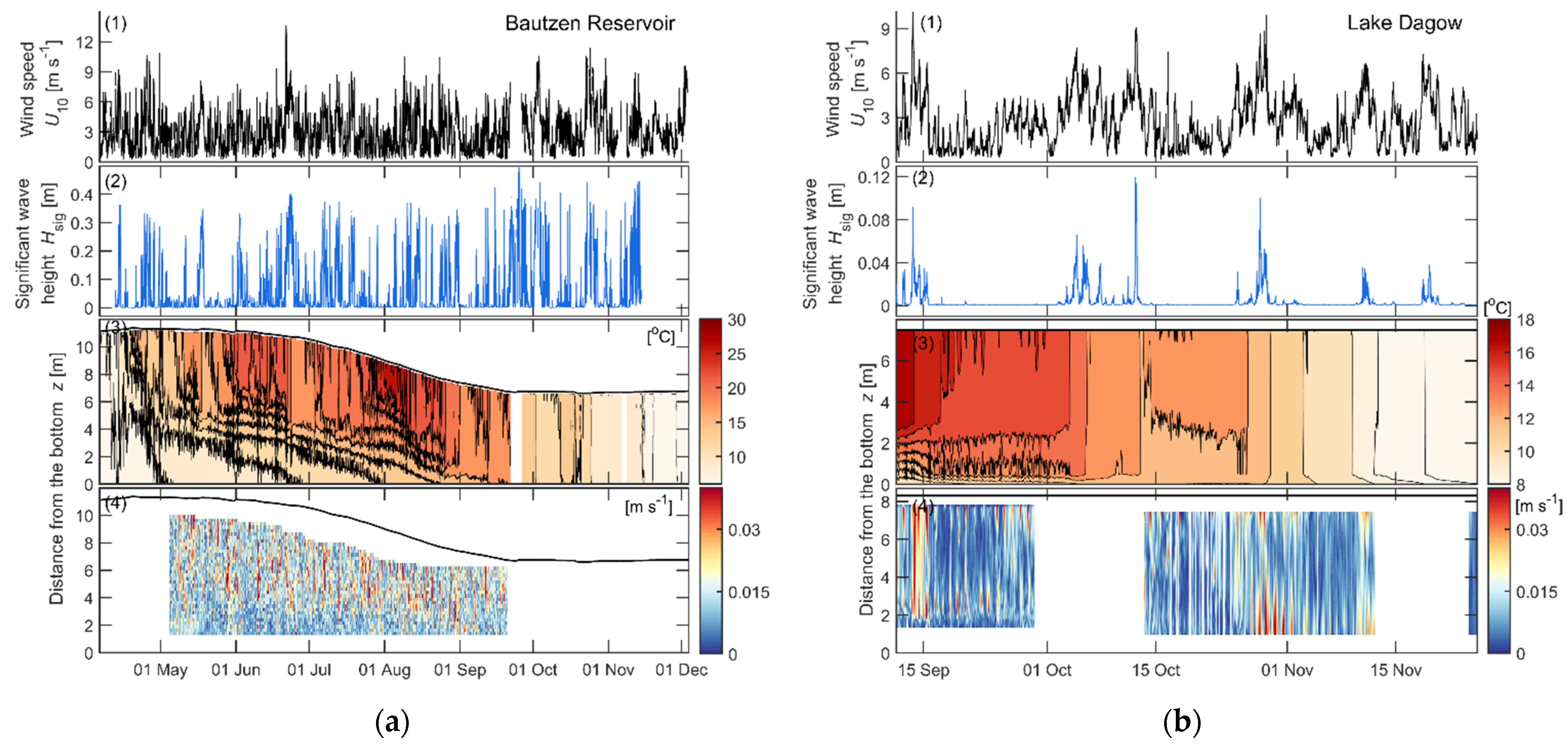
Figure 3.
Potential energy in stratification and efficiency of energy transfer from wind to water in (a) Bautzen Reservoir and (b) in Lake Dagow. From top to bottom: (1) the black line shows the time series of Schmidt stability (Sc). The horizontal red lines mark the threshold value (5 J m−2) to separate mixed and stratified conditions. (2) Relationship between rate of working RW and wind energy input P10. Gray dots show all data. Red and blue lines represent bin-averages for two selected cases: Sc ≥ 5 and Sc < 5 J m−2—indicating stratified and mixed conditions, respectively. A minimum of 5 data points was considered for the bin-averaging. The black line shows a linear regression for all data with P10 < 2 W m−2. Inset graphs in the lower panels show a detailed view of the data at small energy fluxes. The slope coefficient, i.e., the efficiency of energy transfer from wind to water is equal to (1.3 ± 0.1) × 10−3 and (2.61 ± 0.05) × 10−3 for Bautzen Reservoir and Lake Dagow, respectively.

Figure 4.
(a) Significant wave Hsig as a function of wind speed . Lines with markers represent measurements: black color shows data from [18]. Blue, green and red colors represent the bin-averaged data from the present study: Bautzen Reservoir A (platform), B (shore) and Dagow Lake G (shore). Solid lines show a commonly applied empirical parameterization of the significant wave height based on the wind speed and fetch length (JONSWAP). The parameterization was applied to the observed wind speed and direction with a resolution of 30 min. (b) Boxplots showing the percentages of the ratio of wave energy flux per unit length of wave crest (Pwave) to the fetch-integrated wind energy flux (approximated as P10 multiplied by the fetch length) for three measurement locations. The central horizontal line in boxes indicates the median; the bottom and top edges of the boxes denote the 25th and 75th percentiles; the whiskers extend to the largest data points which are not considered outliers.
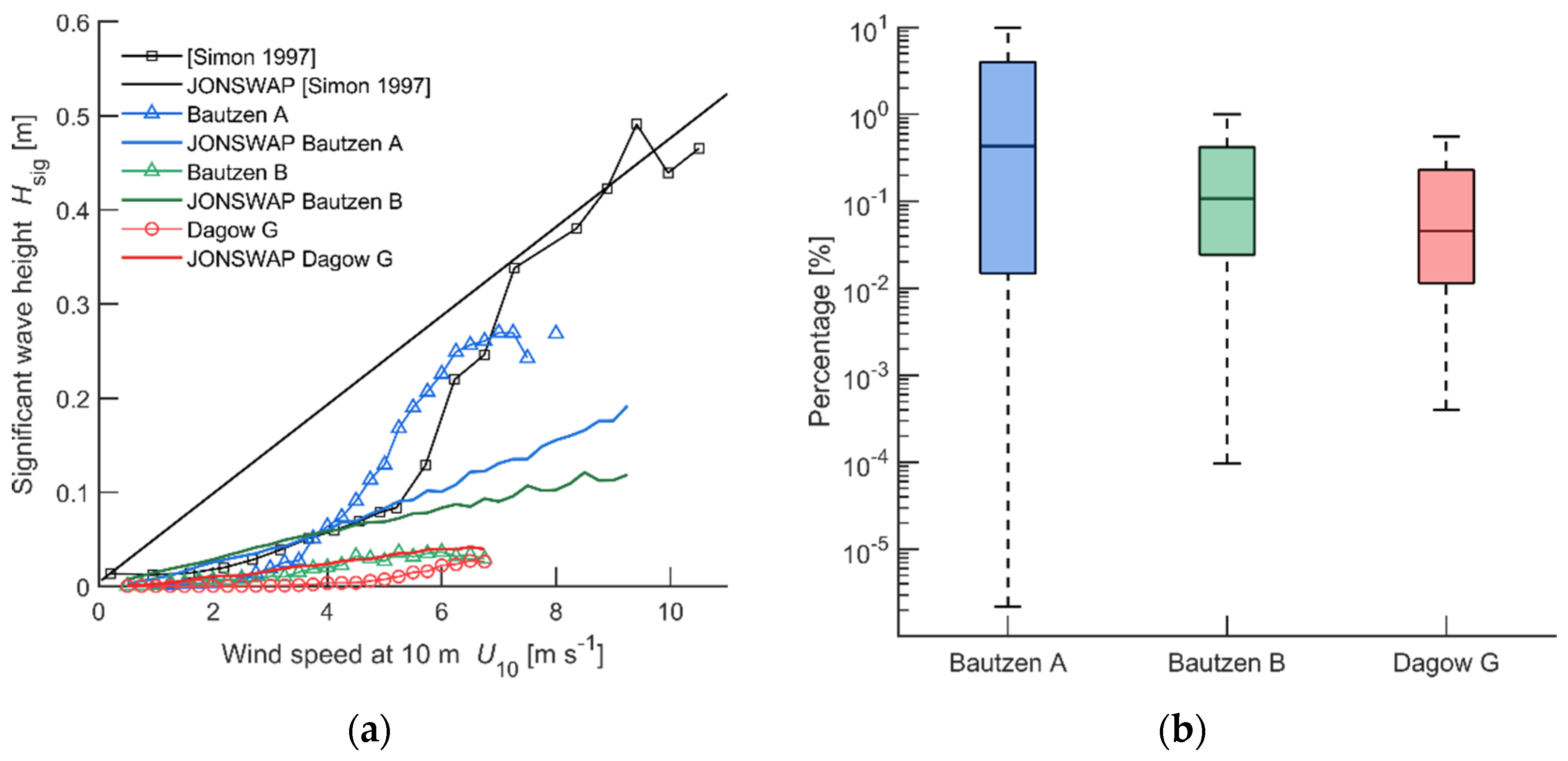
Figure 5.
(a) Sample data from Bautzen Reservoir illustrating high-frequency internal waves with a period of 6 min (upper panel) and basin-scale internal waves with the period of 9 h (lower panel). The upper and lower panels show vertical (w) and horizontal (u) velocity components, respectively. Black lines show temperature isotherms; blue lines show the distance above the bed for which the velocity power spectra are shown in panel (b). (b) Power spectral density estimates for flow velocity components (m2 s−1) and isotherms (m2 s). Blue, light blue and red solid lines show velocity spectra; gray, black and light red show isotherm spectra for Bautzen Reservoir and Lake Dagow, respectively. Internal waves are associated with distinct spectral peaks and vertical dashed lines denote major internal wave periods.
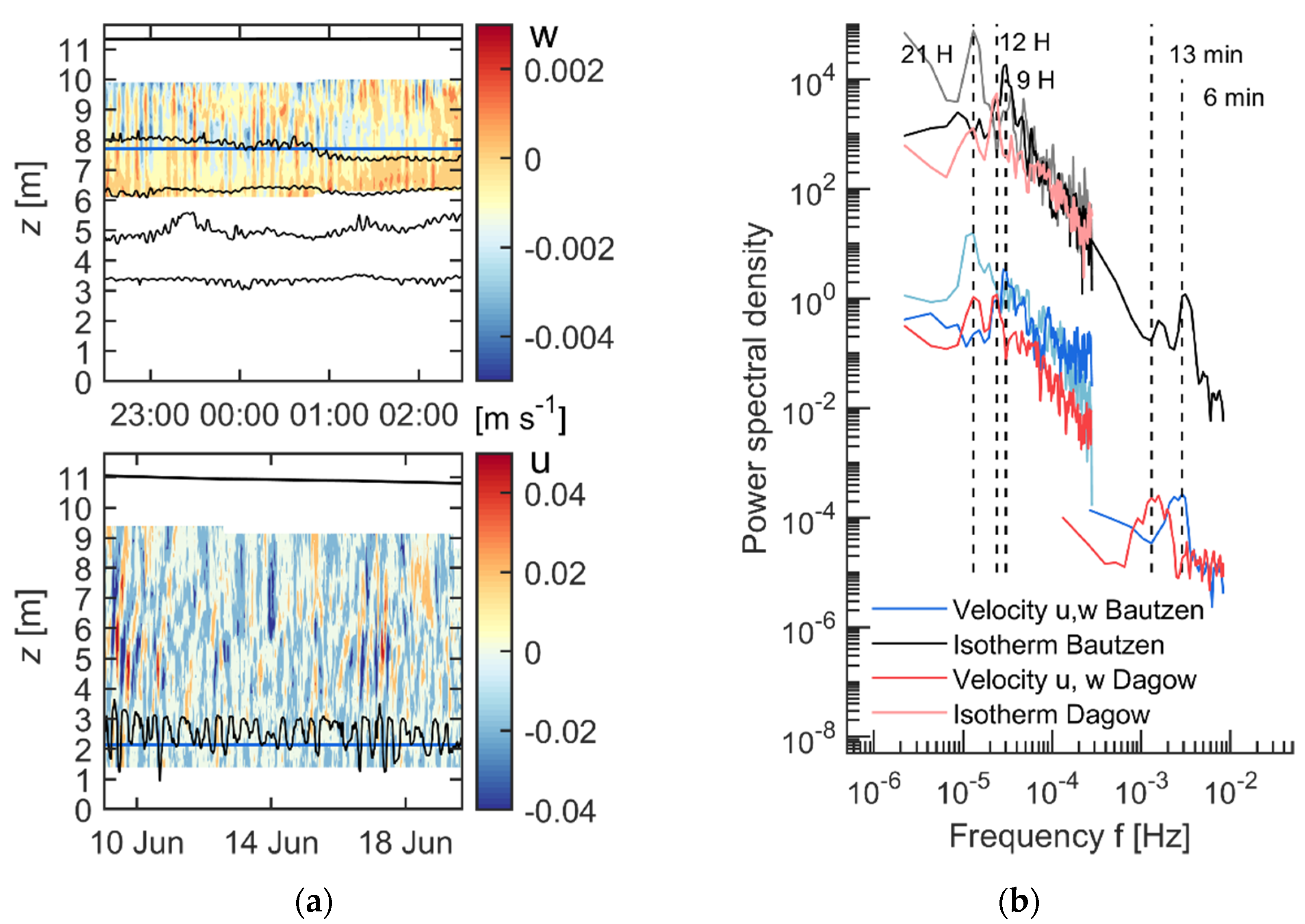
Figure 6.
(a) Average available potential energy (APE) in basin-scale internal waves (upper panel) and in high-frequency internal waves (lower panel) throughout the measurement period in Bautzen Reservoir. The red-shaded areas correspond to the presence of the basin-scale waves with 8–9 h period, the green-shaded area shows the presence of a wave with 21 h period. The width of the bars is not to scale but is proportional to the event duration (i.e., narrow bars indicate shorter events where waves are present, and wider bars indicate longer events). The black line in the lower panel (a) shows a moving average of the APE. (b) Sample data demonstrating the transfer of wind energy to basin-scale internal waves. The upper panel shows the time series of P10 and APE averaged over one wave cycle. After the wind event stopped, APE grows first and then decays after three wave cycles. The lower panel shows isothermal depths with the event duration marked by red vertical lines.

Figure 7.
Vertical profiles of log-averaged energy dissipation rates (ε) for all available data (gray and red shaded areas show the 5th to 95th range of data): (a) combined data with dissipation rates calculated using the structure function and inertial subrange fitting methods (black circles, the platform-mounted ADCP facing downward) and using bottom boundary layer approach (see Section 2.4, red circles, the ADCP deployed at the bottom) in Bautzen Reservoir. The vertical axis is split into two subaxes with identical scaling: The lower axis corresponds to the distance from the bottom, the upper—to the distance from the surface. Thus, we avoid averaging over the entire water column because the water level change was significant throughout the measurements. Data are based on measurements in Bautzen Reservoir. (b) Dissipation rate calculated using the structure function method and the BBL approach based on measurements in Lake Dagow (separately for the first and for the following two ADCP deployment periods).

Figure 8.
Scheme showing mean energy fluxes in (W m−2) and mean energy content (J m−2) for the two studied water bodies. Numbers written before/after a slash correspond to the values obtained from Bautzen Reservoir and Lake Dagow measurements, respectively. Solid and dashed lines illustrate the motion and equilibrium positions of vertical layers of water with the same density.


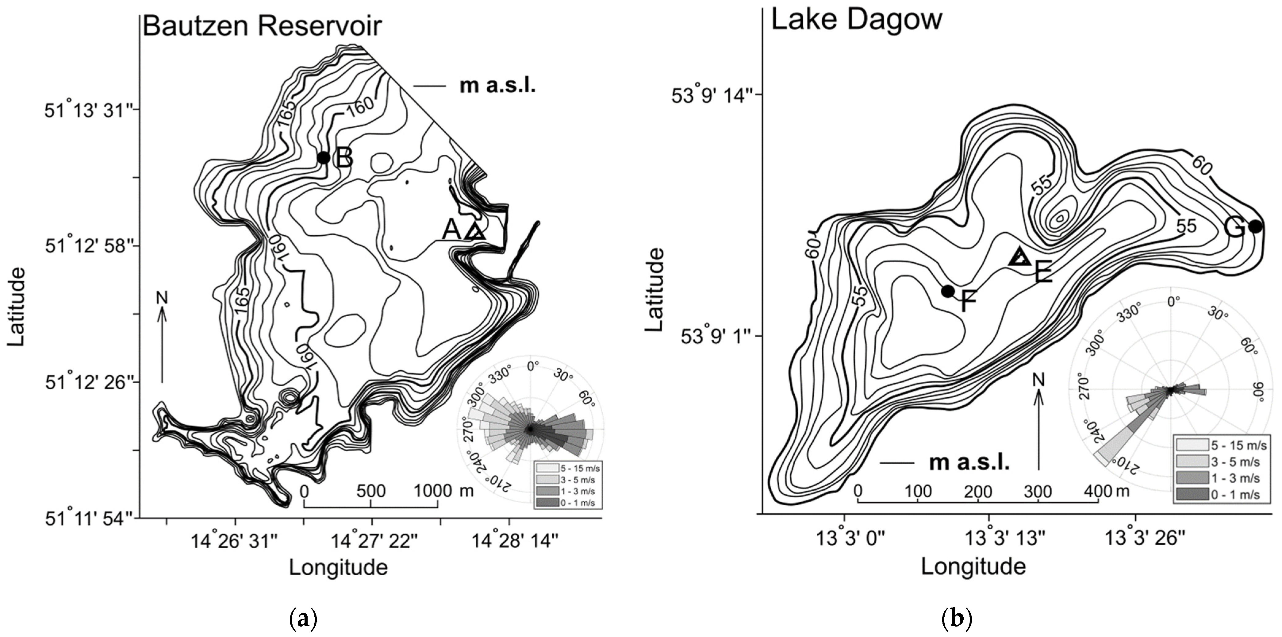
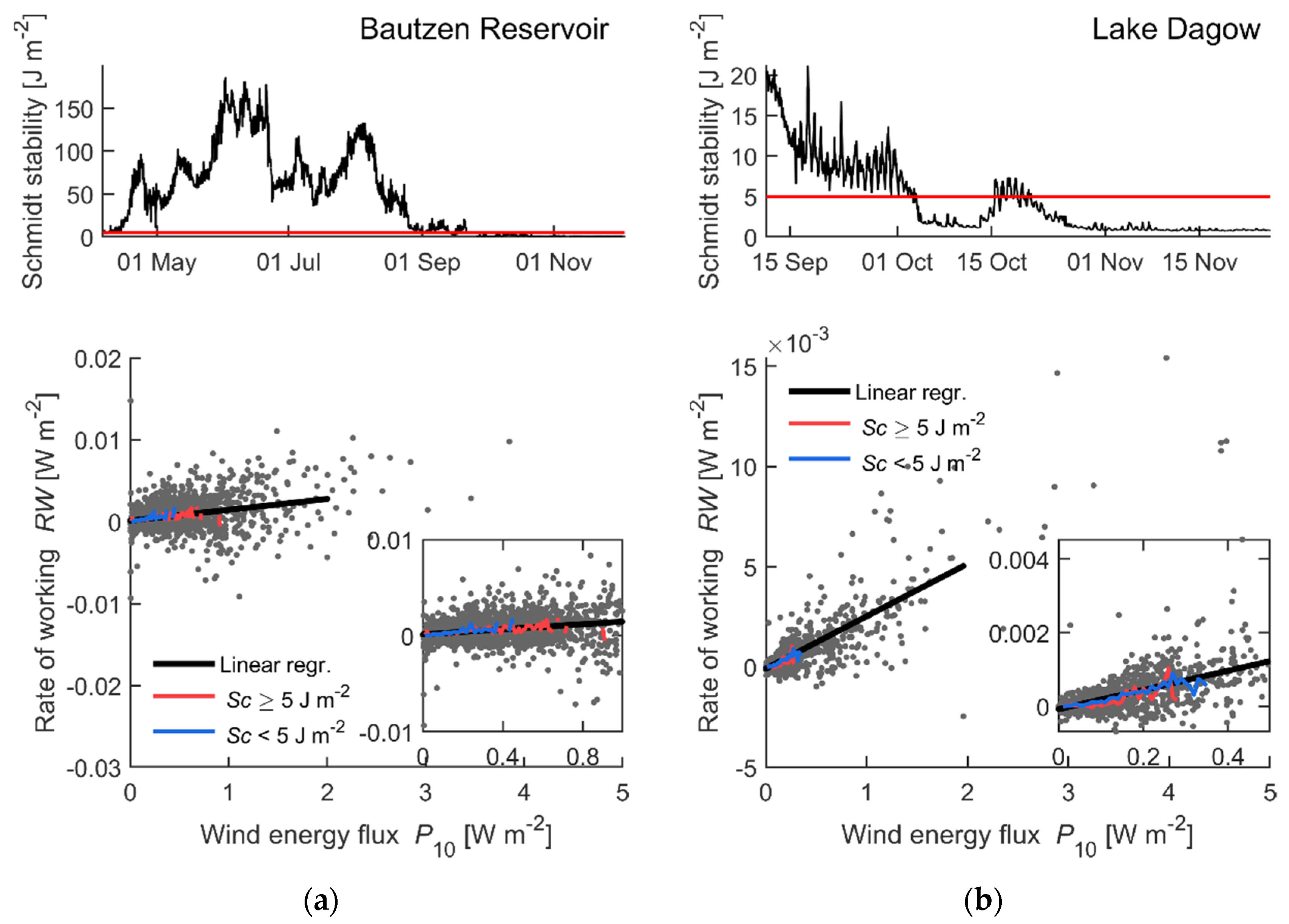
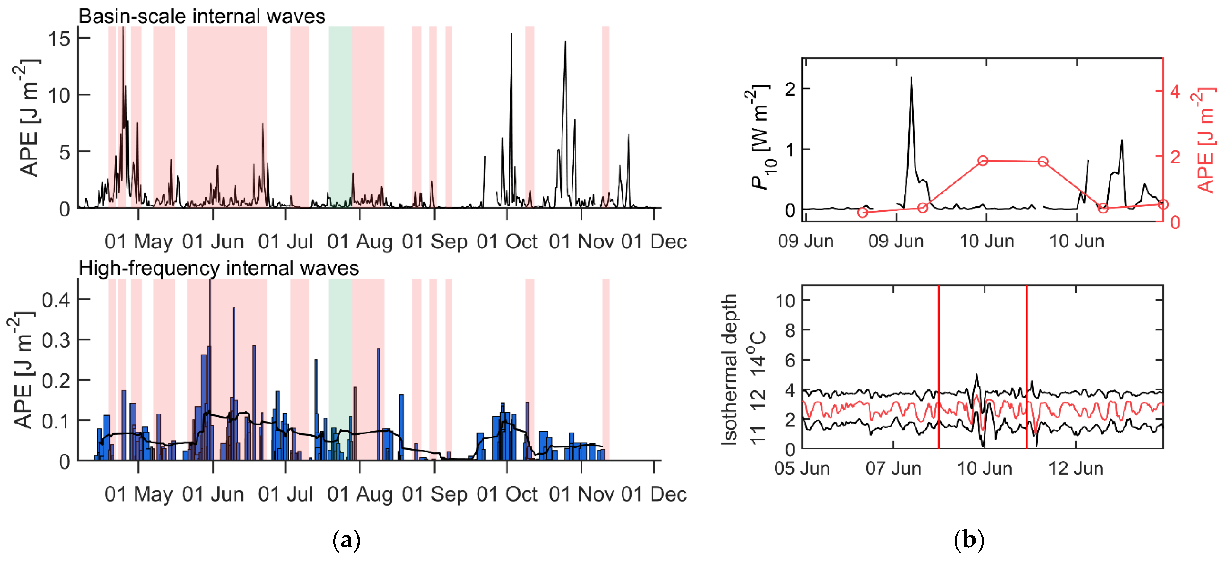
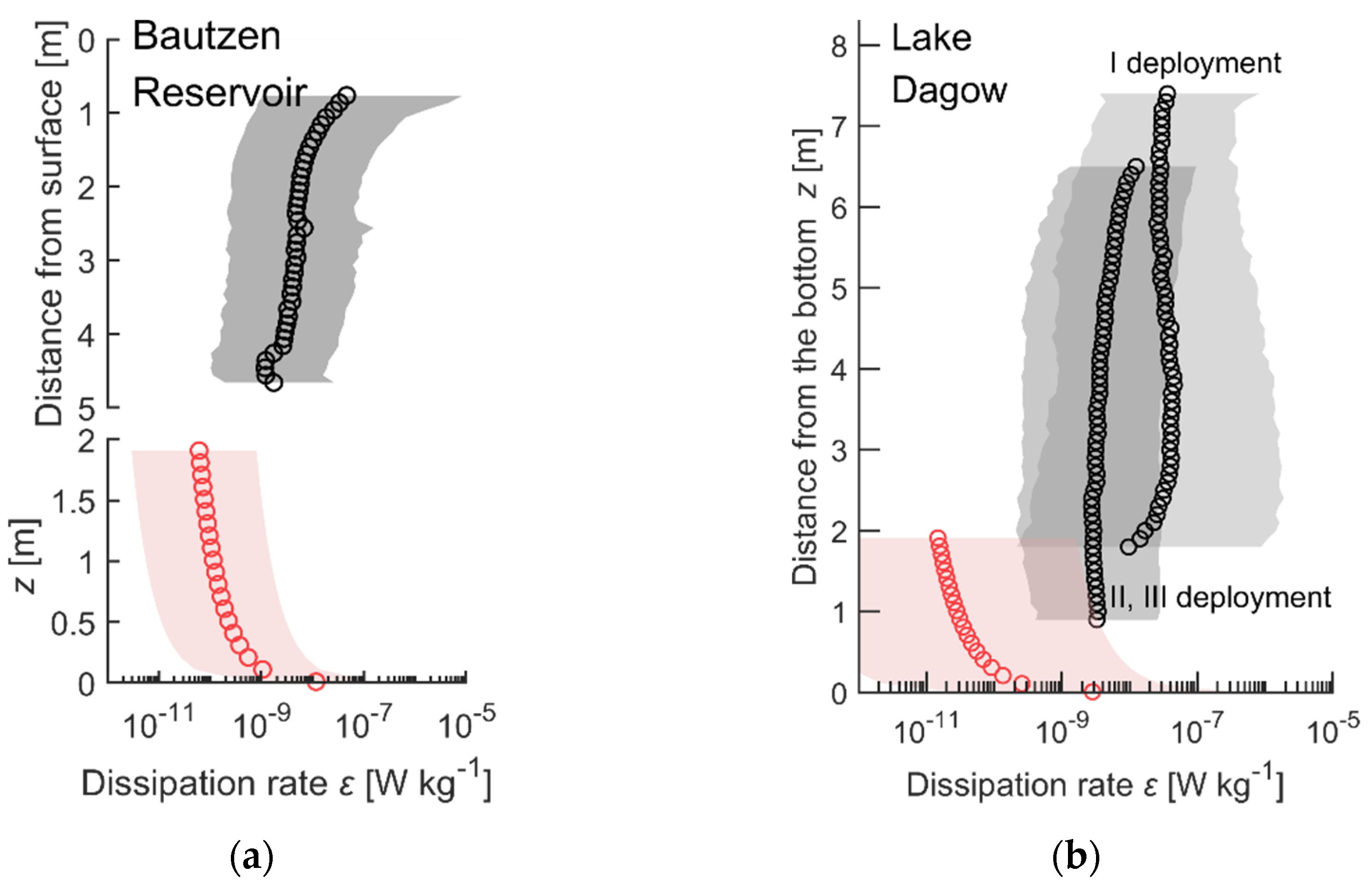
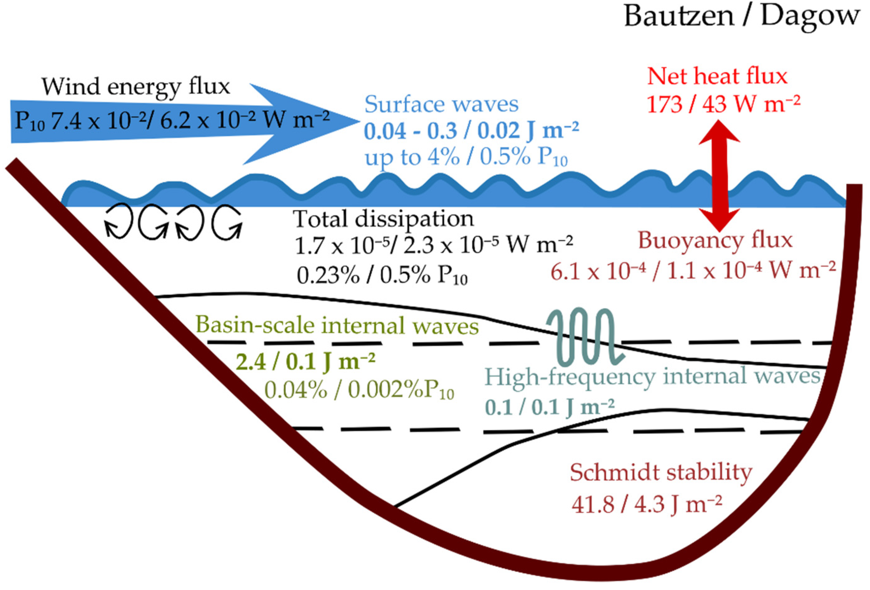
Table 1.
Instrumentation and resolution for the water-side and atmospheric measurements conducted in Bautzen Reservoir and Lake Dagow.
Table 1.
Instrumentation and resolution for the water-side and atmospheric measurements conducted in Bautzen Reservoir and Lake Dagow.
| Type of Measurements | Water Body | Instrument | Resolution | Location on the Map (Figure 1) |
|---|---|---|---|---|
| Flow velocity | Bautzen Reservoir | (a) ADCP RDI Workhorse 600 kHz (range: 1.4–10 m); (b) Workhorse 1200 kHz (range: 0.8–4.7 m) | (a) 10 min with 200 pings with 0.25 m bin size; (b) 1 s with 0.1 m bin size | (a) Bottom deployment (facing upward) ~10 m from southern corner of the platform; (b) platform deployment (facing down, southwest corner) |
| Lake Dagow | ADCP RDI Workhorse 600 kHz (3 deployments, range: (1) 0.5–6.8 m; (2–3) 0.8–7.1 m) | 5 s with 12 pings with 0.1 m bin size | 3 deployments: (1) platform (facing down, west corner), point E; (2–3) ~6–7 m from northern corner of the platform (facing upward) | |
| Water temperature | Bautzen Reservoir | (a) Thermocouples (type T, Copper/Constantan) | 10 min averages from measurements in 30 s intervals | Platform, point A |
| Lake Dagow | RBR solo | 10 s | Point F | |
| Wave measurements | Bautzen Reservoir | RBR duet | 10 min with 512 measurements of 16 Hz | Platform, point A; shore, point B |
| Lake Dagow | Shore, point G | |||
| Wind speed | Bautzen Reservoir | Campbell Scientific, CSAT3 (1.8 m) | 20 Hz, as well as 10 min and 30 min averages | Platform, point A |
| Lake Dagow | Gill Instruments HS-50 (1.97 m) | 20 Hz | Platform, point E | |
| Radiation | Bautzen Reservoir | Kipp and Zonen, CNR1 | 10 and 30 min averages from measurements in 30 s intervals | Platform, point A |
| Lake Dagow | Kipp and Zonen, CNR4 | measured at 1 Hz, logged at 1 min averages | Platform, point E |
Publisher’s Note: MDPI stays neutral with regard to jurisdictional claims in published maps and institutional affiliations. |
© 2021 by the authors. Licensee MDPI, Basel, Switzerland. This article is an open access article distributed under the terms and conditions of the Creative Commons Attribution (CC BY) license (https://creativecommons.org/licenses/by/4.0/).
Share and Cite
MDPI and ACS Style
Guseva, S.; Casper, P.; Sachs, T.; Spank, U.; Lorke, A. Energy Flux Paths in Lakes and Reservoirs. Water 2021, 13, 3270. https://doi.org/10.3390/w13223270
AMA Style
Guseva S, Casper P, Sachs T, Spank U, Lorke A. Energy Flux Paths in Lakes and Reservoirs. Water. 2021; 13(22):3270. https://doi.org/10.3390/w13223270
Chicago/Turabian StyleGuseva, Sofya, Peter Casper, Torsten Sachs, Uwe Spank, and Andreas Lorke. 2021. "Energy Flux Paths in Lakes and Reservoirs" Water 13, no. 22: 3270. https://doi.org/10.3390/w13223270
Note that from the first issue of 2016, this journal uses article numbers instead of page numbers. See further details here.