An Alternative to Laboratory Testing: Random Forest-Based Water Quality Prediction Framework for Inland and Nearshore Water Bodies

Abstract

Water quality monitoring plays a vital role in the water environment management, while efficient monitoring provides direction and verification of the effectiveness of water management. Traditional water quality monitoring for a variety of water parameters requires the placement of multiple sensors, and some water quality data (e.g., total nitrogen (TN)) requires testing instruments or laboratory analysis to obtain results, which takes longer than the sensors. In this paper, we designed a water quality prediction framework, which uses available water quality variables (e.g., temperature, pH, conductivity, etc.) to predict total nitrogen concentrations in inland water bodies. The framework was also used to predict nearshore seawater salinity and temperature using remote sensing bands. We conducted experiments on real water quality datasets and random forest was chosen to be the core algorithm of the framework by comparing and analyzing the performance of different machine learning algorithms. The results show that among all tested machine learning models, random forest performs the best. The data prediction error rate of the random forest model in predicting the total nitrogen concentration in inland rivers was 4.9%. Moreover, to explore the prediction effect of random forest algorithm when the independent variable is non-water quality data, we took the reflectance of remote sensing bands as the independent variables and successfully inverted the salinity distribution of Shenzhen Bay in the Google Earth Engine (GEE) platform. According to the experimental results, the random forest-based water quality prediction framework can achieve 92.94% accuracy in predicting the salinity of nearshore waters.

1. Introduction

Presently, the world is facing a crisis of freshwater shortage. Rivers are the most common source of freshwater, but along with industrial development, human activities have damaged the river water environment [1]. Domestic sewage, industrial wastewater, and agricultural drainage all contain inorganic salts such as nitrogen and phosphorus which may adversely affect the water quality of the river [2]. The shortage of freshwater resources is often not a lack of water, but a lack of clean water. Through sensors or laboratory testing, water quality monitoring can help us develop water quality management measures to protect water resources and improve aquatic habitats [3]. Water managers use different tools to monitor water quality, such as using sensors to monitor the physical characteristics of water [4], analyzing the biochemical characteristics of water in the laboratory [5], and even monitoring water bodies through satellite technology [6].

However, traditional monitoring means have redundancy in the arrangement of sensors, with one sensor needing to be placed for each water quality parameter. This placement strategy may result in a waste of resources. Moreover, the cost of monitoring different water quality indicators varies. For example, basic indicators such as temperature, pH, and conductivity can be monitored quickly and easily by sensors at a very low cost. Indicators such as total nitrogen (TN), on the other hand, require laboratory testing to produce accurate results, which is not only time-consuming but also costly [7]. As rivers are very mobile and water quality changes rapidly, traditional methods may not perform well in terms of timeliness in responding to changes in water quality if the tests take longer. In addition, these monitoring are often carried out separately, and the intrinsic link between the results obtained from these monitoring methods is ignored. For example, in inland rivers, total nitrogen is required to be measured in the laboratory, but because of the link between it and other features that are easily obtained through sensors, we can develop a framework to exploit that link. Simply put, total nitrogen concentration data can be obtained without laboratory or specialized detection instruments. This is also true in nearshore waters, where the large area of the nearshore sea makes the placement of a large number of sensors impractical, while satellite remote sensing technology provides a means of monitoring over a large spatial and temporal range. If we use the optical characteristics of seawater, establish the link between water quality and remote sensing reflectivity [8] and use this link to invert the water quality of a large area, we can realize the dynamic monitoring of nearshore waters. Therefore, the study and use of the relationship between different water quality indicators can be used to indirectly predict specific water quality indicators. This kind of predictive tools can contribute to water environment management [9].

Due to the highly dynamic nature of river water status, the collection and analysis of water quality data may not meet the dynamic requirements. With the extensive use of sensors, many water quality studies have adopted the “surrogate-regression” approach [10], which allows analysis of water quality by external factors. For example, using discharge, turbidity, conductivity, etc. to estimate the nutrient status of the water body [11], or directly using environmental proxies to estimate [12]. Most of the studies that used the “surrogate-regression” method employed simple linear regression or multiple linear regression [13,14,15]. However, the reality is that the relationship between water quality data is not linear, but nonlinear. To address this problem, many scholars have used machine learning methods to explore nonlinear relationships among variables and have successfully applied machine learning methods to water-related fields: for example, flood prediction [16], river flow [17], groundwater pollution [18], photophysiology [19], etc.

In recent years, with the development of big data technology in the field of water quality prediction, machine learning has also been applied to river monitoring [20]. The methods used include Random Forest (RF) [21], Recurrent Neural Network (RNN) [22,23], Support Vector Machine (SVM) [24], etc. Dissolved oxygen (DO) [25], chlorophyll (Chl-a) [26], total phosphorus (TP) [27], and ammonia nitrogen ( $N{H}_3-N$) [28] in water are used as variables to be predicted. In addition to using the relationship between physical and biochemical indicators in water, satellite remote sensing data are also widely used to predict water quality [29,30,31]. Google earth engine (GEE) is a platform that can be used to perform large-scale remote sensing calculations and is very friendly for studying land and ocean [32,33,34]. With GEE, we can use pre-trained models to predict the land parameters [35] and the water parameters [36] by remote sensing data.

However, we found that existing studies have not paid enough attention to the prediction of total nitrogen (TN) concentration in inland water bodies. In particular, total nitrogen concentrations in rivers reflect the degree of eutrophication. Excess nitrogen in rivers provides nutrients for algae, and most river ecosystems are unable to carry the abnormal and excessive rate of growth of these algae. Eutrophication occurs when algae bloom in large quantities in a short period of time. Algae that exceed the carrying capacity of a river can consume almost all of the dissolved oxygen in the river, causing other aquatic organisms in the river to die due to lack of oxygen. [37]. Monitoring of nitrogen in rivers is done mainly using sensor monitoring and laboratory testing [9].

In this paper, a random forest-based prediction framework is designed to enrich methods of water quality monitoring for inland and nearshore water quality. Two water bodies were studied in this study: inland rivers and nearshore waters. These two water bodies have different characteristics and there are differences in the analysis. Through the proposed framework with different data sources as input and target predicted water quality parameters as outputs, the results of experiments validate the robustness of the framework. The main contents of the study are as follows:

• We explored the relationship between different water quality indicators and designed a water quality prediction framework, which uses machine learning methods to predict the target variable water quality indicators by the dependent water quality parameters
• We compared the performance of different kinds of machine learning methods for total nitrogen (TN) prediction in the inland river and the best performing model was selected to be the core algorithm of the prediction framework
• We discussed the feasibility of the proposed framework for water quality inversion with water surface reflection data acquired by remote sensing. The GEE platform was used to solve the problem of big data calculation and to map the salinity distribution of nearshore water bodies.

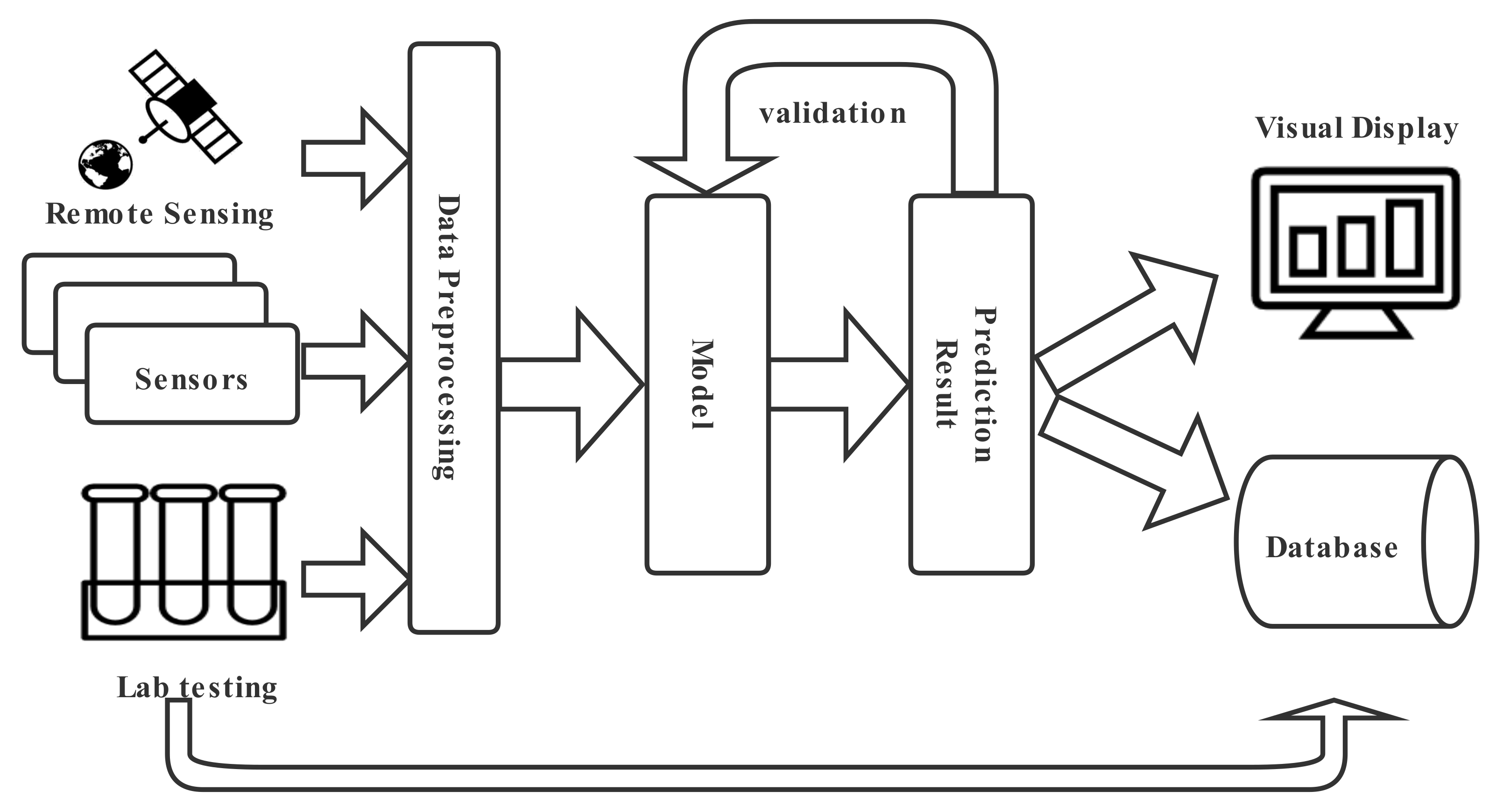
2. Framework for Inland and Nearshore Water Quality Prediction

Based on the above situation, we designed the water quality prediction framework as shown in Figure 1. As can be seen, the framework is divided into three parts, from left to right are: raw data acquisition and processing, model training and prediction, storage and display.

2.1. Data Acquisition and Pre-Processing

For different waters and their characteristics, the raw data are acquired in different ways. For example, in predicting the water quality of inland water bodies, the raw data mainly comes from the sensors installed at the water quality monitoring stations in the early stage. A small part of the data that is difficult to obtain directly through the sensor is obtained through laboratory analysis after a certain frequency of water quality sampling. In the nearshore sea water quality prediction, the original data include not only the water quality management department sampling and testing data, but also satellite transmission to the ground remote sensing data. Because the frequency of detection and sampling is different, and water quality prediction requires the correspondence of relevant data, so the original data need to be pre-processed. Prediction of inland and nearshore water quality, the independent variable data used is also different. To the inland river total nitrogen prediction, for example, the independent variables used are other water quality indicators with correlation. The nearshore seawater quality prediction using remote sensing reflectance data as the independent variable.

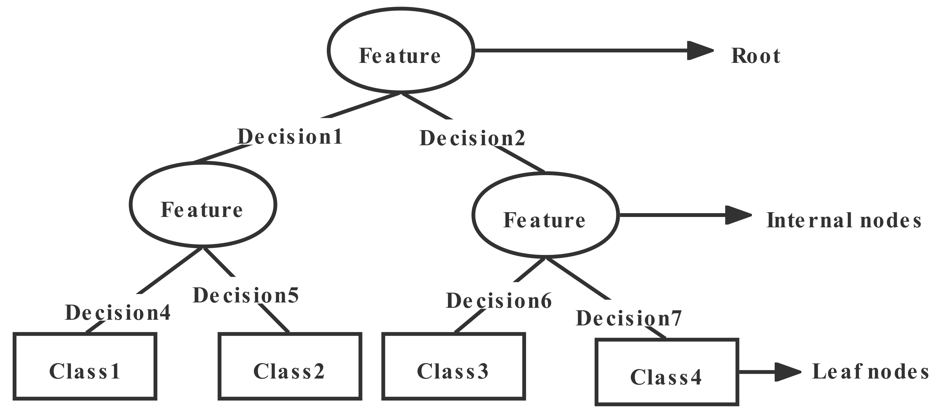
2.2. Decision Tree and Random Forest Model

The idea of the framework is to employ machine learning methods to predict water quality. Models learn the linear or nonlinear relationships that exist between the data from the training set. The trained models then make predictions on the test set data to test the model’s effectiveness and generate evaluation metrics. Since there are nonlinear relationships between total nitrogen and other water parameters (such as temperature and pH), these factors directly affect the growth of algae in water bodies and indirectly affect the concentration of TN in waters. It is the existence of this nonlinear relationship that gives the possibility to predict TN. We consider the task of predicting TN as a mathematical regression problem. Here, we use the random forest as the prediction model for the whole framework.

2.2.1. Decision Tree

Decision tree is the basic structure of many ensemble learning methods, called classification tree when used for classification and regression tree when used for regression [38]. Unlike other classification methods that combine a set of features in a single decision step to perform classification, decision trees are based on a multi-stage or hierarchical decision scheme or tree structure and consist of nodes and directed edges. A decision tree consists of two types of nodes: internal nodes and leaf nodes. A feature or attribute of the data is represented by an internal node, while a leaf node represents a class. Specifically, a leaf node represents the result of a decision from the root node to this leaf node, and an internal node represents the data classification test performed at that point, i.e., the feature or attribute to which the test data belongs. Each node of the decision tree structure makes a binary decision, and the samples contained in the node based on the result of the attribute test are divided into sub-nodes (the root node contains the full set of samples), and the path from the root node to each leaf node corresponds to a sequence of decision tests. This processing is usually performed by moving down the tree until a leaf node is reached. In the decision tree approach, the characteristics of the data (i.e., other water parameters) are predictor variables, while the class to be mapped (TN) is referred to as the target variable. The tree-like structure of a decision tree is shown in Figure 2.

The key to decision trees is how to divide the data set with the expectation of making the unneeded data more orderly, and the measure of orderliness and disorderliness is information entropy:

$$H\left(X\right)=-\sum _{\kappa =1}^K{P}_{\kappa }ln{P}_{\kappa }$$

(1)

where X denotes the sample set containing K categories and $P_{\kappa }$ denotes the proportion (frequency) of the κ-th sample in the sample set D. Taylor expansion of $f\left(x\right)=-lnx$ at $x=1$ (ignoring higher order infinitesimals):

$$\begin{array}{cc}f\left(x\right)\hfill & =f\left(x_0\right)+f^{\prime }\left(x_0\right)(x-x_0)+O\hfill \\ \hfill & =f\left(1\right)+f^{\prime }\left(1\right)(x-1)+O\hfill \\ \hfill & =1-x\hfill \end{array}$$

(2)

Thus, the entropy can be translated as:

$$\begin{array}{cc}\hfill H\left(X\right)\hfill & \hfill =-\sum _{\kappa =1}^K{P}_{\kappa }ln{P}_{\kappa }=\sum _{\kappa =1}^K{P}_{\kappa }(-ln{P}_{\kappa })\hfill \\ \hfill \hfill & \hfill \approx \sum _{\kappa =1}^K{P}_{\kappa }(1-P_{\kappa })=Gini\left(X\right)\hfill \end{array}$$

(3)

Here, Gini (X) refers to the Gini index. Although decision tree is not an ensemble learning method, it is the basis of random forest and gradient boosted decision tree.

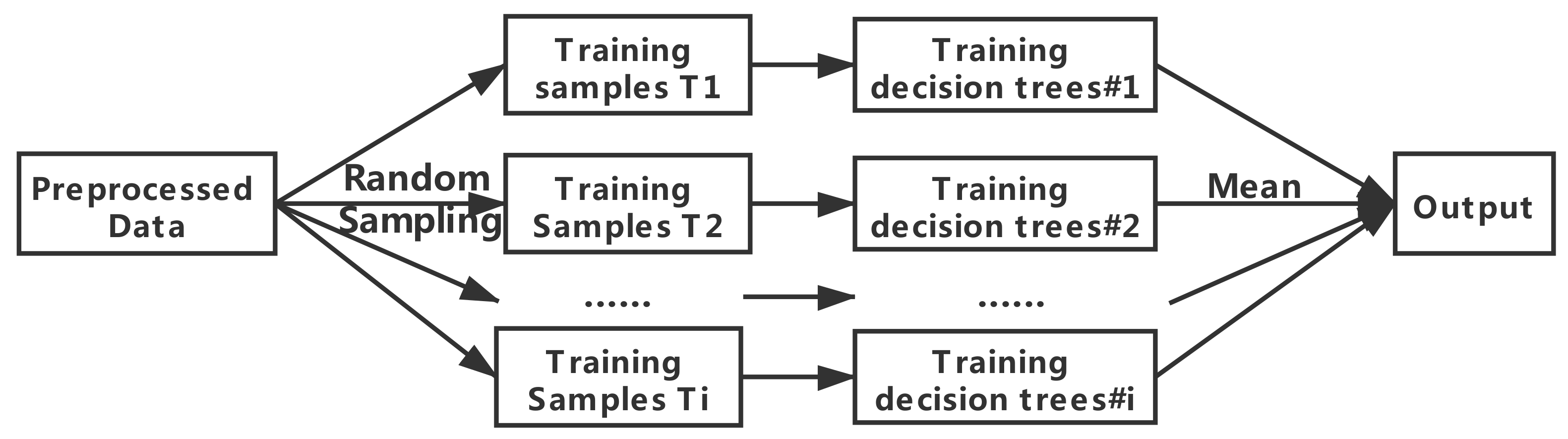
2.2.2. Random Forest

The idea of random forest is to build a forest of several decision trees and merge them together to have more accurate and stable results. Random forest contains two aspects of randomness. First, the selection of samples is random: a certain number of samples are drawn from the training set to generate the root node samples of the classless decision tree. Second, the selection of attributes is random: during the construction of each decision tree, a certain number of candidate attributes are randomly selected, from which the most suitable attribute is chosen as the split node. The random forest model randomly resamples the input data set, generates multiple training sets to construct decision trees, and then determines the final prediction based on the results (majority or average) of all decision trees. Figure 3 shows the training process of random forest.

The basic steps of the random forest algorithm are as follows:

• Sampling: From the training set T, K sets of data sets are generated by Boostrasp sampling with put-back. Each set of data sets is divided into two kinds of sampled data and un-sampled data (out-of-bag data), and each data set will generate a decision tree by training.
• Growth: Each decision tree is trained by training data. At each sub-node, m features are randomly selected from M attributes, and the optimal features are selected based on the Gini metric for full branching growth until no more growth is possible, without pruning.
• Testing: Using the out-of-bag data to test the accuracy of the model. Because out-of-bag data are not involved in modeling, model effects and generalization capabilities can be tested to some extent. The prediction error of out-of-bag data is picked up to determine the best decision tree in the algorithm and re-modeled.
• Prediction: Using the determined model for new data and prediction, the average of all decision trees prediction results is the final output.

3. Case Studies of Inland and Nearshore Water Quality

As mentioned previously, the research in this paper was conducted in inland waters and nearshore waters. In inland waters, we use the designed framework to predict river total nitrogen concentrations through relationships between water quality parameters; in nearshore waters, we invert seawater temperature and salinity using the reflectance of seawater to light observed by satellite.

3.1. Experiment Description and Settings

The experiments are conducted according to the proposed framework. All experiments in this article are compiled and tested on Windows system (CPU: Inter(R) Core(TM) i7-9700K CPU @ 3.60 GHz; GPU: Inter(R) UHD Graphics 630). All codes are written using the syntax of Python 3.8. The pre-processed data will be split into training set (90%) and testing set (10%). After processing the real water quality data, random forest is used as the core algorithm to learn the nonlinear relationships existing between water quality variables in the training set. The test set is used to evaluate the performance of the model.

3.2. Baseline Methods

In our experiment, to verify that random forest outperforms other common machine learning algorithms in inland and nearshore water quality prediction tasks, several methods such as SVR, KNN, Ridge Regression, MLP, Gradient Boosted Regression Tree (GBRT), and Bagging were also used in the study. These methods are described as follows:

3.2.1. SVR

Support vector regression (SVR) is an application of support vector machine (SVM) [39,40] for regression of continuous variables [41]. The idea of SVR is that given dataset A of D elements $\{(X_i,y_i)i=1,2,\dots ,D\}$, d represents the sample of the training set, and $X_i$ is the i-th element of the d-dimensional vector, i.e., $X_i=\{x_1,x_2,\dots ,x_d\}\in {\Re }^d$, and $y_i\in \Re$ is the actual value corresponding to $X_i$. The target output function of the SVR can be quantified by the following equation:

$$F\left(x_i\right)={\omega }^T\varphi \left(x\right)+b=\sum _{i=1}^T{w}_i\varphi \left(x_i\right)+b$$

(4)

where $\omega$ is the weight vector, ${\omega }_i$ and b are coefficients determined by minimizing the error between the network output and the target variable, and $\varphi \left(x_i\right)$ is the nonlinear mapping function. In practical applications, $\varphi \left(x_i\right)$ is replaced by the kernel function $K(x,z)$.

3.2.2. KNN

The K nearest neighbor(KNN) model is a nonparametric method proposed by Thomas Cover [42] that can be used for classification and regression. The output of the KNN model depends on the operation to be performed, for regression purposes, the model predicts an actual value, called the attribute value of the new data point. The input to the model is the nearest N neighboring data points, and the Euclidean distance between the new data point and its N nearest neighbors is calculated.

3.2.3. Ridge Regression

Ridge regression is a popular parameter estimation method used to address the collinearity problem frequently arising in multiple linear regression [43,44]. When there is covariance in the equation variables, a change in one variable can also cause other variables to change. Ridge regression is the addition of a constant matrix to the original equation that produces bias but ensures the stability of the regression coefficients. Although this addition results in a loss of information, it can be exchanged for a reasonable estimate of the regression model.

3.2.4. MLP

Multilayer Perceptron (MLP) [45] is a feed-forward neural network implementation that mimics the connectivity between human neurons, where the neurons between layers are connected in a fully connected manner. The hidden layer receives the signals from the input layer nodes and converts them into signals sent to all output nodes, converting them into the final layer output. The error between simulation and observation is minimized using a back-propagation algorithm. Activation function is used to enhance the network’s ability to express nonlinear regression relationships.

3.2.5. Gradient Boosted Regression Tree

Gradient Boosted Regression Tree (GBRT), a model based on decision tree regression, can handle nonlinear and complex relationships between data. GBRT is an iterative decision tree algorithm that consists of multiple decision trees, and the final result is the cumulative sum of the conclusions of all trees [46]. GBRT uses a forward distribution algorithm, which minimizes the loss function by selecting the appropriate decision tree function based on the current model and the fitted function.

3.2.6. Bagging

The basic idea of Bagging Tree [47] is to consider that part of the output error in a single regression tree is due to a specific selection of the training dataset. Bagging uses self-sampling to generate different base classifiers. It introduces self-sampling to obtain training subsets for training base classifiers. Each sample training set is used to train a base learner, and the mean of all weak learner results is the output of Bagging regression.

3.3. Evaluation Methodology

Different models perform differently on data prediction. To compare the performance of various machine learning models on total nitrogen concentration prediction, we used $MAE$ (Mean Absolute Error), $MSE$ (Mean Square Error), $RMSE$ (Root Mean Square Error), $NSE$ (Nash–Sutcliffe efficiency coefficient), and $MAPE$ (Mean Absolute Percentage Error) as metrics to evaluate the models.

• MAE:

  $$MAE=\frac{1}{m}\sum _{i=1}^m|y_i-f\left(x_i\right)|$$

  (5)
• MSE:

  $$MSE=\frac{1}{m}\sum _{i=1}^m{(y_i-f\left(x_i\right))}^2$$

  (6)
• RMSE:

  $$RMSE=\sqrt{\frac{1}{m}\sum _{i=1}^m{(y_i-f\left(x_i\right))}^2}$$

  (7)
• MAPE:

  $$MAPE=\frac{1}{m}\sum _{i=1}^m\frac{|y_i-f\left(x_i\right)|}{y_i}\ast 100\%$$

  (8)
• $NSE$:

  $$NSE=1-\frac{{\sum }_{i=1}^m{(y_i-f\left(x_i\right))}^2}{{\sum }_{i=1}^m{(y_i-\overline{y})}^2}$$

  (9)

where m is the number of data, $y_i$ is the observed values, $f\left(x_i\right)$ is the predicted values, and $\overline{y}$ is the average of $y_i$.

MAE, MSE, RMSE, and MAPE are used to measure the gap between the observed and model-predicted values. The larger the value of the indicator, the larger the difference between the true and predicted values, and the worse the performance of the model. The value of the Nash–Sutcliffe efficiency coefficient ($NSE$) is from negative infinity to 1. The closer the $NSE$ is to 1, the better the model is; the closer it is to 0, the worse the model is. If $NSE$ is much less than 0, then the model is not credible.

3.4. Case Studies of Inland Water Quality

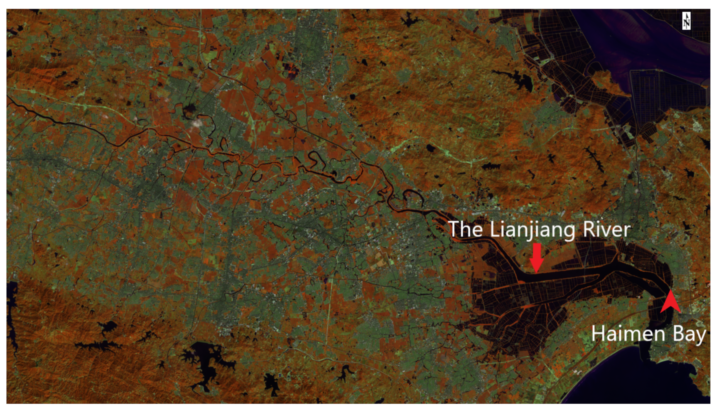
3.4.1. Study Area and Materials

The case study area in Inland Water is the Lianjiang River basin, which is located in the eastern part of China’s Guangdong Province. Lianjiang River has 17 large and small tributaries that join the mainstream from north to south. The main river is 71 km long and has a basin area of 1346.6 km${}^2$. The Lianjiang River is one of the mother rivers of the Chaoshan region and the population in the basin reaches more than 4 million people, a density six times the provincial average. The high population density and intensive industrial enterprises have put enormous pressure on the environment. The local government has invested around $4 billion in the management of the Lianjiang River, which shows the importance of monitoring and management of the river.

Data used in this part are from the water quality monitoring station set up by the Shantou Ecology and Environment Bureau (https://www.shantou.gov.cn/epd/) (accessed on 17 November 2021) in Haimen Bay (23°12${}^{\prime }$45.7${}^{″}$ N, 116°37${}^{\prime }$15.7${}^{″}$ E WGS-84). The geographical location of the Lianjiang River and Haimen Bay can be seen in Figure 4. As shown on the map, the station is located at the mouth of the Lianjiang River, where water quality predictions help to avoid pollution of the sea by inland sewage.

The majority of water quality data collected at the monitoring stations is at two-hour intervals and all nitrogen (TN) data are collected at four-hour intervals. Therefore, the data were collated and data items containing total nitrogen concentrations were retained, for a total of 1917 sets of water quality data. Water quality indicators include temperature (Temp), pH, dissolved oxygen (DO), turbidimetry (Tud), chemical oxygen demand (COD), total dissolved solids (T.D.S), ammonia nitrogen ($N{H}_3-N$), and total nitrogen (TN). The data are statistically described in

Table 1. Several characteristics of water quality data.

	Temp	pH	DO	Tud	COD	T.D.S	${\mathit{NH}}_3-\mathit{N}$	TN
Magnitude	℃	-	mg/L	NTU	mg/L	$\mathsf{\mu }$S/cm	mg/L	mg/L
MAX	35.00	9.43	15.00	500.00	70.10	8895	12.12	14.20
MIN	15.70	6.15	0.09	1.00	7.00	0.00	0.01	1.90
Mean	25.51	7.34	4.78	61.65	25.22	1848	2.60	6.46
Median	25.70	7.31	4.50	52.00	24.90	1271	2.19	5.77
Mode	19.60	7.23	3.55	49.00	21.60	398	0.24	4.72
SD	4.78	0.40	2.46	41.84	7.63	1589	2.12	2.05
Set	1917	1917	1917	1917	1917	1917	1917	1917

.

3.4.2. Data Processing

• Data normalization
  Different evaluation metrics have different magnitudes and units of magnitude [48], for example, the value of conductivity maybe hundreds of times higher than other observed values. Such differences may have an impact on the prediction results. To eliminate the influence of scale between indicators, the Z-score normalization method [49] is used to normalize the filtered data. The normalized data are scaled between 0 and 1, with z-score normalization method is as follows:

  $$X_{norm}=\frac{X-X_{min}}{X_{max}-X_{min}}$$

  (10)

  where $X_{norm}$ denotes the normalized value, X denotes the real monitored value, $X_{min}$ and $X_{max}$ represents the minimum value and the maximum value in the set of data.
• Correlation Analysis
  To find water parameters that are correlated with TN and can be used as independent variables in predicting the TN process, a correlation analysis was performed to extract possible relationships between the parameters. Pearson’s correlation coefficient was used to measure the correlation between water quality indicators. The formula is as follows:

  $$Co{r}_x{}_y=\frac{Cov(X,Y)}{\sqrt{D\left(X\right)}\sqrt{D\left(Y\right)}}=\frac{E\left(\right(X-EX\left)\right(Y-EY\left)\right)}{\sqrt{D\left(X\right)}\sqrt{D\left(Y\right)}}$$

  (11)

  where $Co{r}_{X,Y}$ is the correlation coefficient of the random variables X and Y, $Cov(X,Y)$ is the covariance of the random variables X and Y, E is the mathematical expectation or mean, D is the variance, and $\sqrt{D}$ is the standard deviation.
  The correlation coefficients between other variables and total nitrogen obtained by Equation (11) are shown in

  Table 2. Correlation coefficient between water parameters and TN.

  Parameter	Temp	pH	T.D.S	DO	Tud	${\mathit{NH}}_3-\mathit{N}$	COD	TP	TN
  Coefficient	−0.75	0.12	0.3	0.012	−0.05	0.63	0.47	0.81	1

  . As can be seen in the table, the correlation coefficients of DO, pH, and Tud with TN are small, indicating the low probability of their linear correlation with TN. We also tested the variables with small correlations in the experiment and found that removing these variables would negatively affect the predicted results. One possible explanation is that there may be a nonlinear relationship between these variables and TN. For example, pH affects algal growth and thus changes TN concentrations, while algal growth affects DO concentrations [50]. Although the linear correlation between DO and TN is the lowest in the table, DO is directly related to the life and death of aquatic organisms. Proper DO helps these organisms to survive, while when algal overgrowth occurs, the DO of the water column decreases, organisms die, and microbial decomposition leads to higher TN in the water. Based on this consideration we retained and used these variables. TP was not used as an independent variable because the detection of TP is similar to TN, which requires laboratory analysis.
• Data Validation
  According to the characteristics of machine learning algorithms, we randomly divide the pre-processed 1917 sets of data into training and testing sets, i.e., 90% of the data are used as training set to train the model and 10% are used as testing set to validate the model and calculate the metrics.

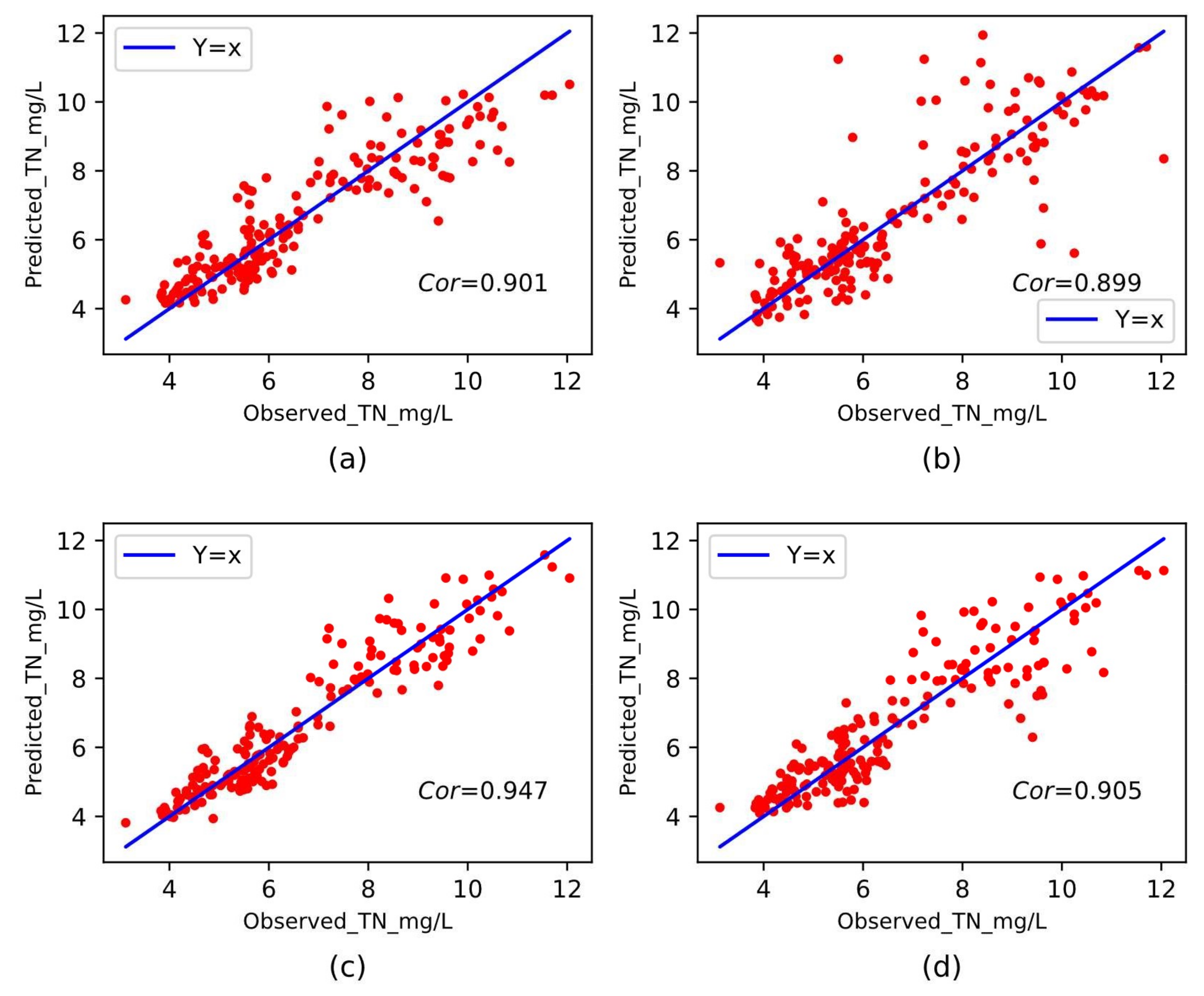
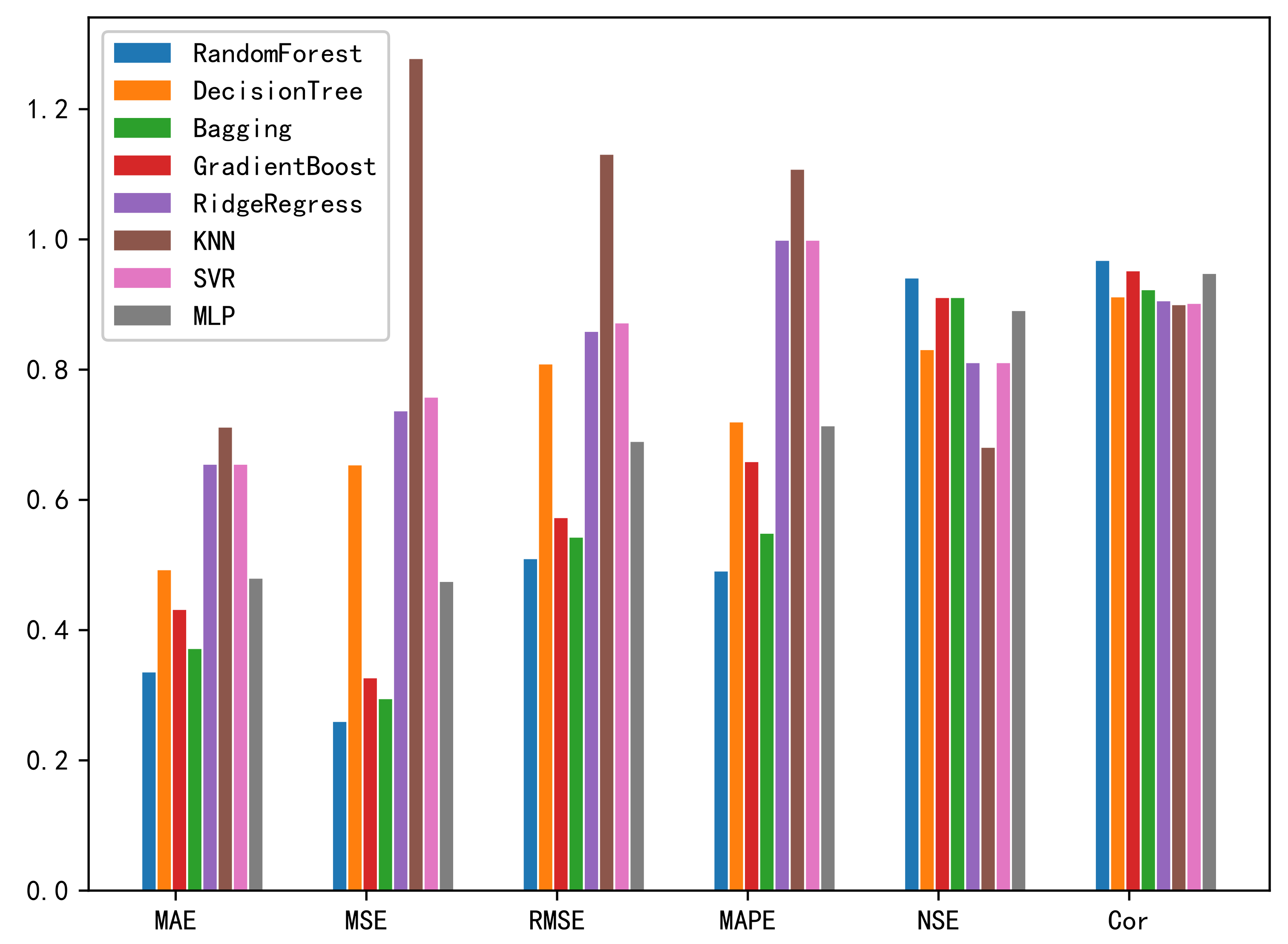
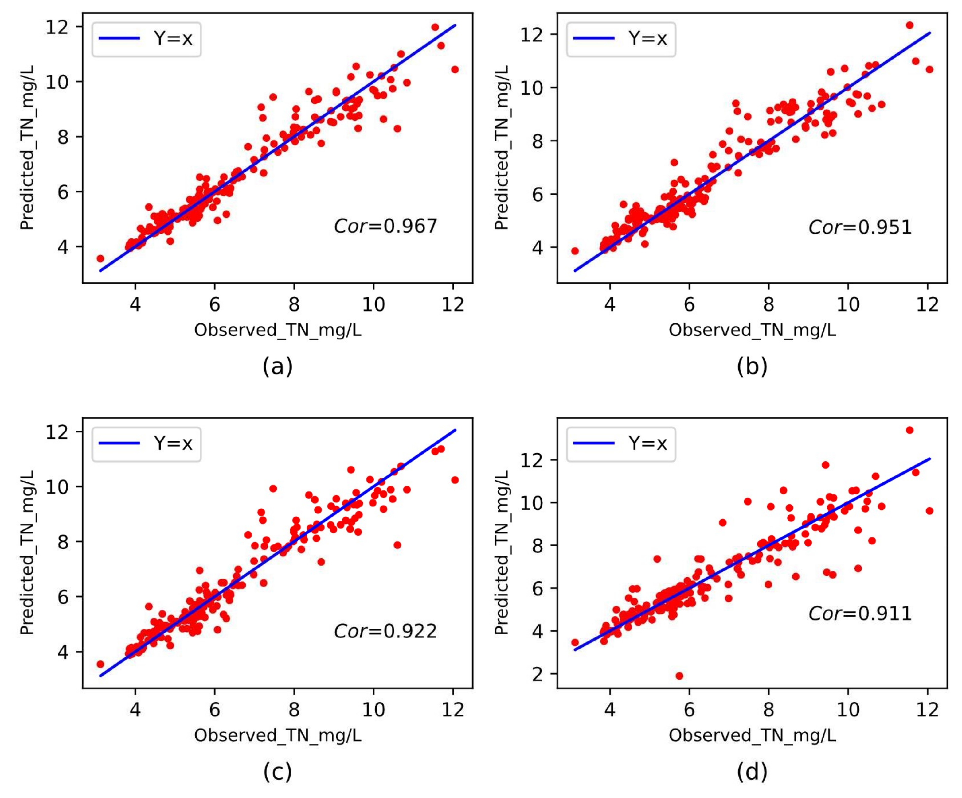
3.4.3. Performance Comparison with Different Baseline Methods

For comparison purposes, we divide the used methods into two categories: ensemble learning methods and non-ensemble learning methods. The ensemble learning methods include Random Forest, Decision Tree, GBRT, and Bagging, while the non-ensemble learning methods include SVR, KNN, Ridge Regression, and MLP.

We calculated the correlation (Cor) coefficients between the predicted and observed values of TN for the Lianjiang River. Scatter plots were drawn with the observed and predicted values as horizontal and vertical coordinates, and we added a diagonal line with $Y=x$ in each plot graph to indicate the result when the prediction is perfect. The deviation of the point from this line reflects the degree of deviation of the predicted value from the observed value. We compared the ensemble learning method and the non-ensemble learning method separately, and then analyzed the model with the best prediction ability in detail.

Figure 5 shows the scatter distribution of the predicted and observed values of the four non-ensemble learning methods. It can be seen that among the four methods, MLP has the smallest deviation from the straight line $Y=x$ with the largest correlation coefficient of 0.947, and KNN has the largest deviation from the straight line with the smallest correlation coefficient of 0.899. This indicates that the neural network performs better in the TN concentration prediction task in the study area compared with other non-ensemble learning methods. In addition, we found that the points determined by the predicted and observed values are closer to the straight line $Y=x$ when the TN concentration is small.

Figure 6 shows the scatter distribution of the predicted and observed values of the four ensemble learning methods. It can be seen that the correlation coefficients between the predicted and observed values of the four ensemble learning methods are all greater than 0.91, with Random Forest having the largest correlation coefficient of 0.967. The correlation coefficients of Gradient Boosting are 0.951, Bagging 0.922, and Decision Tree 0.911, all of which are greater than those of SVR, KNN and Ridge Regression. The deviation of the points in the scatter plot from the straight line $Y=x$ is smaller than that of the three non-ensemble learning methods mentioned above, which indicates that the predicted values of the ensemble learning methods are closer to the observed values in the task of predicting TN concentrations in inland rivers. In the comparison with the baseline method, random forest has the best performance.

Table 3. Evaluation results for predicting inland water quality.

	$\mathrm{MAE}$	$\mathrm{MSE}$	$\mathrm{RMSE}$	$\mathrm{MAPE}$	$\mathrm{NSE}$	$\mathrm{Cor}$
MLP	0.479	0.474	0.689	7.13%	0.89	0.947
SVR	0.654	0.757	0.871	9.98%	0.81	0.901
KNN	0.711	1.277	1.13	11.07%	0.68	0.899
RidgeRegress	0.654	0.736	0.858	9.98%	0.81	0.905
GradientBoost	0.431	0.326	0.572	6.58%	0.91	0.951
Bagging	0.371	0.294	0.542	5.48%	0.91	0.922
Decision Tree	0.492	0.653	0.808	7.19%	0.83	0.911
RFR	0.335	0.259	0.509	4.90%	0.94	0.967

shows the results of these eight methods on the six evaluation metrics, in which we use bold fonts to highlight the best performance results. By category, both the data fitting ability and the accuracy of prediction ensemble learning methods perform better than non-ensemble learning methods. The experimental results indicate that random forest performs the best among the eight methods. The MAE = 0.335, MSE = 0.259, RMSE = 0.509, and MAPE = 4.9% of random forest are the lowest among the methods; $NSE$ = 0.94 and $Cor$ = 0.967 are the highest among the methods, which indicates that the fitting ability of the random forest is stronger than other methods and the prediction error is smaller than other methods. From Table 3, it can be seen that random forest improves the prediction accuracy by about 2 times compared with non-ensemble learning methods. The prediction accuracy of random forest is also higher than that of decision trees, gradient boosting trees, and Bagging, which are also ensemble learning methods. This shows that our proposed framework is better than these baseline methods in terms of prediction accuracy.

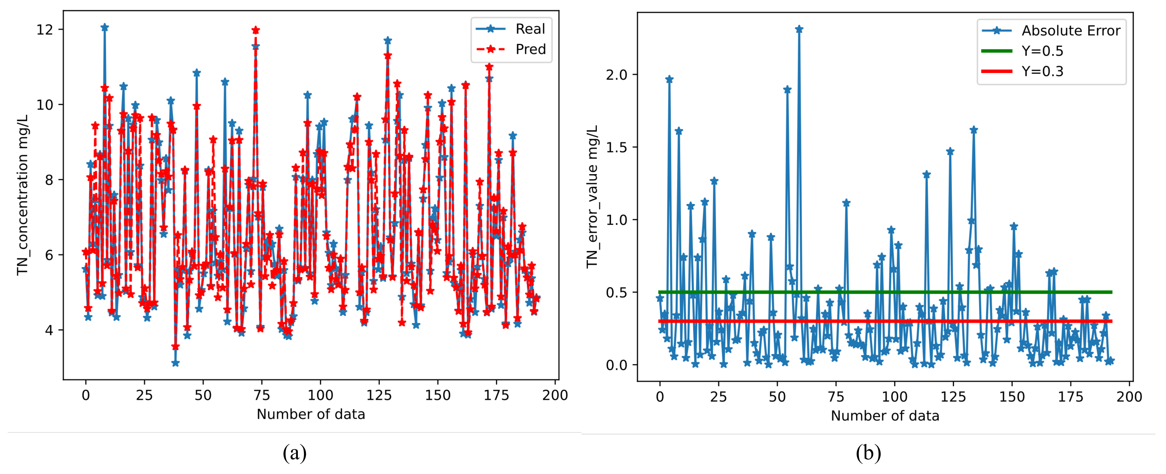
3.4.4. Prediction Results of The Framework for TN

After comparing the performance of the model, we use the random forest as the core algorithm of the framework to predict the TN at the monitoring site of Haimen Bay, and the comparison of the predicted results with the true values is shown in Figure 7a. Most of the predicted values are very close to the observed values, which also indicates the good performance of the model. However, there are still some cases where the difference from the true value is large, which is due to the fact that these raw data with large errors in the test set are some large values. For example, the error rate is 10% for all, and the error for a concentration of 14 mg/L is 1.4 mg/L, while the error for a concentration of 6 mg/L is 0.6 mg/L which is less than half of 1.4 mg/L.

Figure 7b shows the absolute error between the predicted and observed values of TN. After the prediction of the test set data, we counted the range of these absolute errors. A total of 120 out of 192 data sets had absolute error values less than or equal to 0.3 mg/L, accounting for 62.5%, and 153 out of 192 data sets had absolute error values less than or equal to 0.5 mg/L, accounting for 79.7%. The mean absolute error (MAE) of the test set was 0.335 mg/L.

3.5. Case Studies of Nearshore Water Quality

Remote sensing technology is generally used to observe light-sensitive features, such as land, vegetation, and forest fire sites. In the field of watercolor remote sensing, the research objects are usually chlorophyll-a, soluble solids, yellow substances, etc., and there are fewer studies on non-optical sensitive objects in the water. Seawater salinity is very important for marine organisms and is a key indicator for maintaining the ecological balance of the ocean [51]. To a certain extent, the dynamic balance of seawater salinity reflects the stability of marine ecosystems. Since the effects of human activities on seawater salinity are mainly concentrated in nearshore waters, it is of great interest to monitor seawater salinity using the proposed water quality prediction framework.

Like the inland water quality prediction experiments, we use the random forest as the core algorithm of the prediction framework and the other seven machine learning methods as comparisons. The difference is that the source of input data used as the independent variable of the model in nearshore water quality prediction is not the same as inland water quality prediction.

3.5.1. Data Description and Processing

In the nearshore water quality prediction, the study area is Shenzhen Bay (22°29${}^{\prime }$21.7″ N, 113°58${}^{\prime }$46.0″ E WGS-84). Remote sensing data were used as independent variables and water quality data were used as dependent variables. Shenzhen Bay is a river inlet located between Shenzhen City, mainland China and Hong Kong Special Administrative Region, China. The area is densely populated with frequent human activities and has a large impact on the marine ecology. This part of the experiment was done with the GEE platform. Sentinel-2 remote sensing reflectance data of Shenzhen Bay waters from 2018–2019 were downloaded from the GEE platform, and seawater quality data were obtained from the Hong Kong Environmental Protection Department (EPD https://cd.epic.epd.gov.hk/EPICRIVER/marine/, accessed on 17 November 2021).

The raw dataset contains 10 bands, temperature, and seawater salinity data from 11 monitoring sites in Shenzhen Bay. To eliminate the influence of clouds on the reflectance data, a Cloudmask operation was performed using the QA60 band provided by Sentinel-2 SR data. The QA60 band is used in binary form to indicate the presence or absence of clouds at the point, e.g., the tenth binary bit indicates transparent clouds the tenth indicates cirrus clouds if the binary bit is 0 indicates the presence of clouds, and 1 indicates the absence of clouds. Therefore, we set the filtering condition as the tenth and eleventh bits are 0, we can filter out the points without clouds. Due to the inconsistency between satellite transit time and water sampling time, the data were screened, and the minimum time difference was selected to match the data, and 147 sets of data were finally obtained.

As mentioned in the inland water quality prediction, we analyzed the correlation of reflectance data (B with numbers representing bands) with temperature and salinity data, and the decomposition results are shown in

Table 4. Correlation coefficients between temperature, salinity and remote sensing bands.

	B11	B12	B2	B3	B4	B5	B6	B7	B8	B8A
Temperature	0.51	0.50	0.49	0.45	0.48	0.52	0.57	0.57	0.54	0.56
Salinity	−0.65	−0.65	−0.62	−0.68	−0.74	−0.76	−0.69	−0.71	−0.68	−0.68

. We found that the correlation between reflectance data and temperature is positive, and the correlation coefficient is between 0.45 and 0.57. The reflectance data were negatively correlated with the salinity data, and the correlation coefficients ranged from −0.76 to −0.62.

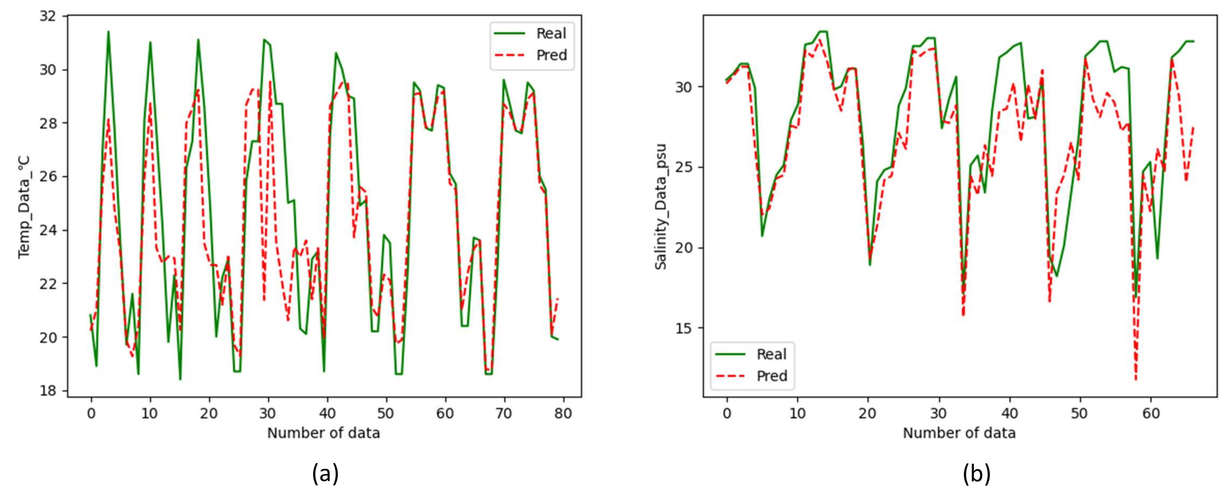
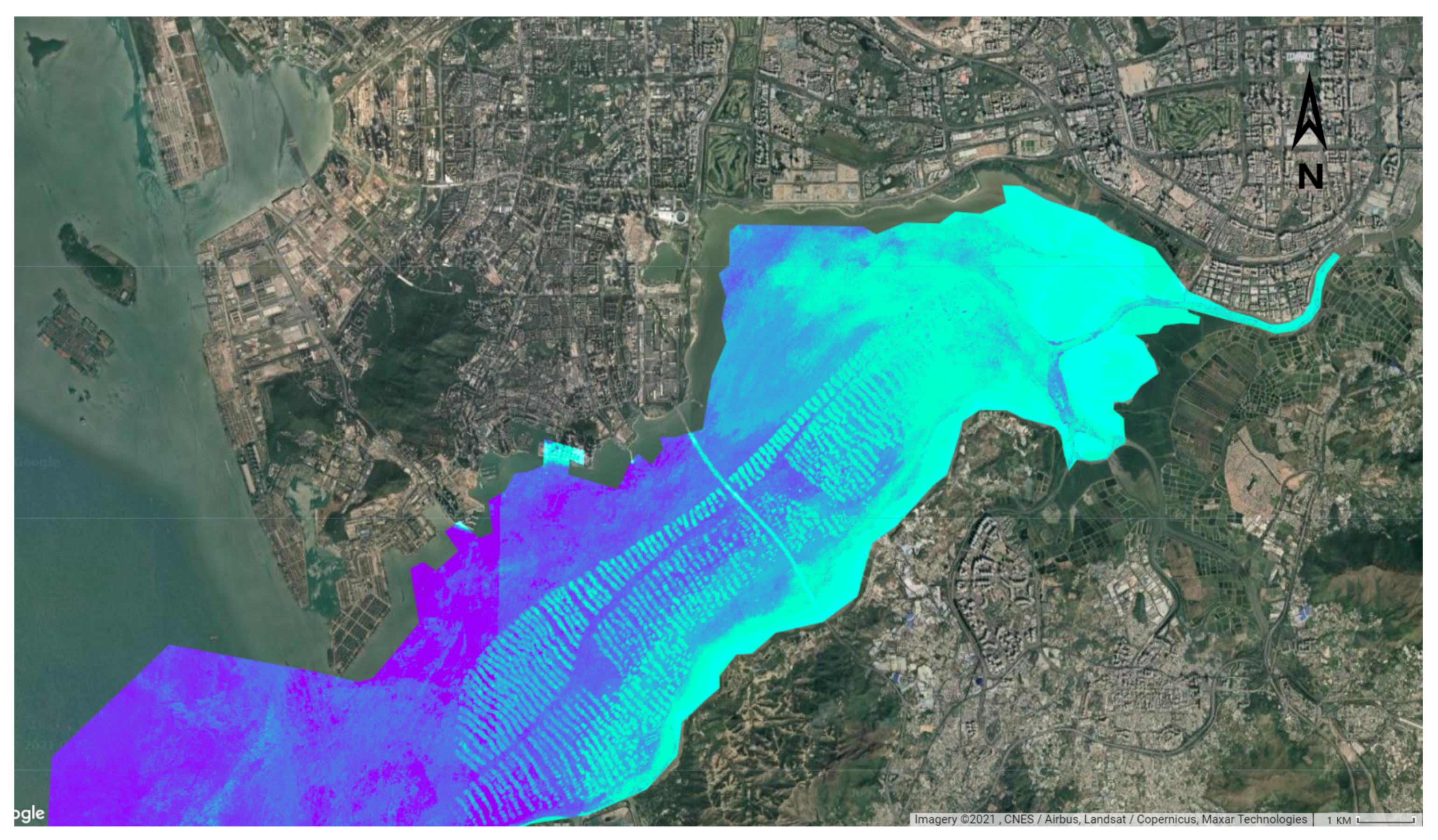
3.5.2. Results of Inversion for Nearshore Water Quality Using Sentinel-2 Data

The regression relationship of remote sensing reflectance with temperature and seawater salinity was established on the GEE platform using the proposed water quality prediction framework. To verify the accuracy and generalization ability of the model, we used the data from six sampling points in the dataset as the training set and the data from the other five sampling points as the test set for the experiments.

As in the comparison experiments in predicting inland water quality, we compared the random forest with the other seven baseline methods on three metrics, $MAE$, $NSE$, and $MAPE$. The results of the comparison are shown in

Table 5. Evaluation results for predicting nearshore water quality.

	Temperature			Salinity
	$\mathit{MAE}$	$\mathit{NSE}$	$\mathit{MAPE}$	$\mathit{MAE}$	$\mathit{NSE}$	$\mathit{MAPE}$
MLP	2.490	0.52	10.83%	1.773	0.76	7.22%
SVR	1.744	0.61	8.42%	2.182	0.61	8.99%
KNN	1.754	0.60	9.45%	2.667	0.62	13.03%
RidgeRegress	2.527	0.51	10.95%	2.165	0.72	8.26%
GradientBoot	1.129	0.77	5.44%	1.887	0.71	7.32%
Bagging	1.337	0.76	5.83%	2.130	0.65	8.47%
Decision Tree	1.620	0.57	6.27%	1.782	0.76	7.23%
RFR	1.107	0.82	4.65%	1.755	0.77	7.06%

. From the table, we can see that the random forest-based prediction framework still performs better than the baseline methods in nearshore water quality prediction.

For the prediction of seawater temperature and salinity in the region, the results of the comparison between observed and predicted values are shown in Figure 8, which shows that most of the predicted values do not differ much from the observed values, and only a few values have error fluctuations. From Table 5, it can be seen that in predicting seawater temperature in the study area, $MAE$ = 1.107 and $MAPE$ = 4.65% for random forest are lower than other methods. Similarly in predicting the salinity of seawater, $MAE$ = 1.755 $MAPE$ = 7.06% for random forest is also the lowest among the experimental methods. This shows the proposed framework is applicable to predict the temperature and salinity of nearshore seawater with good transferability.

Using the visualization tool of the GEE platform, we successfully plotted the salinity distribution of seawater in Shenzhen Bay. As can be seen from Figure 9, the seawater salinity is radially distributed as the water flows from the river to the ocean. This distribution is due to the fact that the outflow from the inland is freshwater with very low salinity and there is a certain dynamic, and with the diffusion effect, the inorganic salts in the high salinity seawater will be transferred to the freshwater with low concentration, so the seawater salinity will gradually increase from the river inlet to the distant sea.

3.6. Discussion

In this study, we first designed a water quality prediction framework and discussed the application of machine learning methods in predicting the inland water quality. Using temperature (Temp), pH, dissolved oxygen (DO), turbidimetry (Tud), chemical oxygen demand (COD), total dissolved solids (T.D.S), and ammonia nitrogen ($N{H}_3-N$) as independent variables, eight machine learning methods were applied to predict the target variable (TN), and $MAE$, $MSE$, $RMSE$, $MAPE$, $NSE$, and $Cor$ were used as the evaluation metrics of model performance. We can visually compare the performance of these methods using Figure 10.

After comparison, we found that the ensemble learning methods and MLP perform better than other non-ensemble learning methods (SVM, KNN, ridge regression). The analysis suggests that due to the complex nonlinear relationships between water parameters, the ensemble learning methods and MLP are better than other non-ensemble methods in capturing the nonlinear relationships between attributes and can optimize the learned features to achieve a better fit. The goal of supervised learning algorithms for machine learning is to learn a stable model that performs well in all aspects. However, practice is often the opposite of expectations. Sometimes we can only obtain multiple models with preferences that may perform better in some aspects. The underlying idea of ensemble learning [52] is to use multiple weak learners so that even if one weak learner produces an incorrect prediction, the other weak learners can fix that error. Ensemble learning can effectively improve the generalization ability of the system. Additionally, due to the introduction of randomness, random forest methods reduce the probability of overfitting cases. Random forest is insensitive to outliers and thus has good noise immunity.

Having obtained the good performance of random forest on river TN prediction task, we try to use remote sensing bands for water quality prediction. Here, seawater temperature and salinity are used as prediction targets, and the independent variables are reflectance data from Sentinel-2 satellite. Then using the computational resources provided by the GEE platform, we successfully inverted the temperature and salinity of the Shenzhen Bay region and plotted the distribution of seawater salinity in the domain. From the distribution map, it can be seen that the seawater salinity increases in a diffuse manner from the river inlet to the outer sea.

4. Conclusions

The purpose of this study is to design a water quality prediction framework and then evaluate the performance of different machine learning methods in water quality prediction. Through the experiments conducted in two different water bodies: inland water and nearshore water, we can draw the following conclusions:

• Machine learning methods and neural network methods can effectively predict the TN in rivers(with an accuracy of 95.1%). Thus, the water quality prediction framework we designed can be used as a soft alternative to sensors in cases where monitoring requirements are less stringent. Research on rivers can provide a real-time and rapid prediction of water quality, which provides a reference basis for river water quality monitoring work, and also provides a decision aid for river management.
• Random forest-based water quality prediction framework can be applied to the inversion of ocean temperature (accuracy reaches 95.35%) and salinity(accuracy reaches 92.94%). Through the reflectance of the water body to light bands, the trained model can invert the water body without the help of water quality data.
• GEE platform is friendly for remote sensing calculation. GEE provides satellite data resources including Landsat series and Sentinel series, and product resources developed with these data. Coupled with its powerful computing power, it can easily solve the problem of large-scale remote sensing calculations.

5. Future Work

When the random forest-based water quality prediction framework is designed, we can apply it in water quality monitoring work. In the future, the framework can be transformed into an online water quality monitoring tool and become part of the monitoring system. Specifically, when the sensor data are in the form of streams as input into the system, the framework can be used to obtain the water quality data that need to be predicted. In the inland water quality monitoring, the work of this paper can not only realize the data prediction of monitoring points without setting TN dedicated sensors, but also be able to fill the data inconsistency due to the different sampling and testing frequency, and provide help for the study of time series and so on. How to achieve the stream data as the input of the model and give prediction results based on this input is the direction of our next work, in which the dynamic update of the model is also a focus of the study.

References

1. Son, G.; Kim, D.; Kim, Y.D.; Lyu, S.; Kim, S. A Forecasting Method for Harmful Algal Bloom (HAB)-Prone Regions Allowing Preemptive Countermeasures Based Only on Acoustic Doppler Current Profiler Measurements in a Large River. Water 2020, 12, 3488. [Google Scholar] [CrossRef]
2. Singh, J.; Yadav, P.; Pal, A.K.; Mishra, V. Water pollutants: Origin and status. In Sensors in Water Pollutants Monitoring: Role of Material; Springer: Berlin/Heidelberg, Germany, 2020; pp. 5–20. [Google Scholar]
3. Jiang, J.; Tang, S.; Han, D.; Fu, G.; Solomatine, D.; Zheng, Y. A comprehensive review on the design and optimization of surface water quality monitoring networks. Environ. Model. Softw. 2020, 132, 104792. [Google Scholar] [CrossRef]
4. Park, J.; Kim, K.T.; Lee, W.H. Recent advances in information and communications technology (ICT) and sensor technology for monitoring water quality. Water 2020, 12, 510. [Google Scholar] [CrossRef] [Green Version]
5. Liu, C.; Zhang, F.; Ge, X.; Zhang, X.; Chan, N.; Qi, Y. Measurement of total nitrogen concentration in surface water using hyperspectral band observation method. Water 2020, 12, 1842. [Google Scholar] [CrossRef]
6. Di Trapani, A.; Corbari, C.; Mancini, M. Effect of the Three Gorges Dam on Total Suspended Sediments from MODIS and Landsat Satellite Data. Water 2020, 12, 3259. [Google Scholar] [CrossRef]
7. Zhao, C.; Chen, L.; Zhong, G.; Wu, Q.; Liu, J.; Liu, X. A portable analytical system for rapid on-site determination of total nitrogen in water. Water Res. 2021, 202, 117410. [Google Scholar] [CrossRef]
8. Zhou, Y.; Yu, D.; Yang, Q.; Pan, S.; Gai, Y.; Cheng, W.; Liu, X.; Tang, S. Variations of Water Transparency and Impact Factors in the Bohai and Yellow Seas from Satellite Observations. Remote Sens. 2021, 13, 514. [Google Scholar] [CrossRef]
9. Ho, J.Y.; Afan, H.A.; El-Shafie, A.H.; Koting, S.B.; Mohd, N.S.; Jaafar, W.Z.B.; Sai, H.L.; Malek, M.A.; Ahmed, A.N.; Mohtar, W.H.M.W.; et al. Towards a time and cost effective approach to water quality index class prediction. J. Hydrol. 2019, 575, 148–165. [Google Scholar] [CrossRef]
10. Robertson, D.M.; Hubbard, L.E.; Lorenz, D.L.; Sullivan, D.J. A surrogate regression approach for computing continuous loads for the tributary nutrient and sediment monitoring program on the Great Lakes. J. Great Lakes Res. 2018, 44, 26–42. [Google Scholar] [CrossRef]
11. Jones, A.S.; Stevens, D.K.; Horsburgh, J.S.; Mesner, N.O. Surrogate Measures for Providing High Frequency Estimates of Total Suspended Solids and Total Phosphorus Concentrations 1. JAWRA J. Am. Water Resour. Assoc. 2011, 47, 239–253. [Google Scholar] [CrossRef] [Green Version]
12. Kuefner, W.; Ossyssek, S.; Geist, J.; Raeder, U. The silicification value: A novel diatom-based indicator to assess climate change in freshwater habitats. Diatom Res. 2020, 35, 1–16. [Google Scholar] [CrossRef]
13. Shah, M.I.; Javed, M.F.; Abunama, T. Proposed formulation of surface water quality and modelling using gene expression, machine learning, and regression techniques. Environ. Sci. Pollut. Res. 2021, 28, 13202–13220. [Google Scholar] [CrossRef]
14. Abba, S.; Hadi, S.J.; Sammen, S.S.; Salih, S.Q.; Abdulkadir, R.; Pham, Q.B.; Yaseen, Z.M. Evolutionary computational intelligence algorithm coupled with self-tuning predictive model for water quality index determination. J. Hydrol. 2020, 587, 124974. [Google Scholar] [CrossRef]
15. Schenk, L.; Bragg, H. Sediment transport, turbidity, and dissolved oxygen responses to annual streambed drawdowns for downstream fish passage in a flood control reservoir. J. Environ. Manag. 2021, 295, 113068. [Google Scholar] [CrossRef] [PubMed]
16. Chang, D.L.; Yang, S.H.; Hsieh, S.L.; Wang, H.J.; Yeh, K.C. Artificial intelligence methodologies applied to prompt pluvial flood estimation and prediction. Water 2020, 12, 3552. [Google Scholar] [CrossRef]
17. Yaseen, Z.M.; El-Shafie, A.; Jaafar, O.; Afan, H.A.; Sayl, K.N. Artificial intelligence based models for stream-flow forecasting: 2000–2015. J. Hydrol. 2015, 530, 829–844. [Google Scholar] [CrossRef]
18. Rahmati, O.; Choubin, B.; Fathabadi, A.; Coulon, F.; Soltani, E.; Shahabi, H.; Mollaefar, E.; Tiefenbacher, J.; Cipullo, S.; Ahmad, B.B.; et al. Predicting uncertainty of machine learning models for modelling nitrate pollution of groundwater using quantile regression and UNEEC methods. Sci. Total Environ. 2019, 688, 855–866. [Google Scholar] [CrossRef] [PubMed]
19. Lucius, M.A.; Johnston, K.E.; Eichler, L.W.; Farrell, J.L.; Moriarty, V.W.; Relyea, R.A. Using machine learning to correct for nonphotochemical quenching in high-frequency, in vivo fluorometer data. Limnol. Oceanogr. Methods 2020, 18, 477–494. [Google Scholar] [CrossRef]
20. Shen, L.Q.; Amatulli, G.; Sethi, T.; Raymond, P.; Domisch, S. Estimating nitrogen and phosphorus concentrations in streams and rivers, within a machine learning framework. Sci. Data 2020, 7, 1–11. [Google Scholar] [CrossRef] [PubMed]
21. Mateo Pérez, V.; Mesa Fernández, J.M.; Villanueva Balsera, J.; Alonso Álvarez, C. A Random Forest Model for the Prediction of FOG Content in Inlet Wastewater from Urban WWTPs. Water 2021, 13, 1237. [Google Scholar] [CrossRef]
22. Chen, Y.; Song, L.; Liu, Y.; Yang, L.; Li, D. A review of the artificial neural network models for water quality prediction. Appl. Sci. 2020, 10, 5776. [Google Scholar] [CrossRef]
23. Xu, J.; Wang, K.; Lin, C.; Xiao, L.; Huang, X.; Zhang, Y. FM-GRU: A Time Series Prediction Method for Water Quality Based on seq2seq Framework. Water 2021, 13, 1031. [Google Scholar] [CrossRef]
24. Mateo Pérez, V.; Mesa Fernández, J.M.; Ortega Fernández, F.; Villanueva Balsera, J. Gross Solids Content Prediction in Urban WWTPs Using SVM. Water 2021, 13, 442. [Google Scholar] [CrossRef]
25. Stajkowski, S.; Zeynoddin, M.; Farghaly, H.; Gharabaghi, B.; Bonakdari, H. A methodology for forecasting dissolved oxygen in urban streams. Water 2020, 12, 2568. [Google Scholar] [CrossRef]
26. Tang, X.; Huang, M. Inversion of chlorophyll-a concentration in Donghu Lake based on machine learning algorithm. Water 2021, 13, 1179. [Google Scholar] [CrossRef]
27. Song, C.M. Application of convolution neural networks and hydrological images for the estimation of pollutant loads in ungauged watersheds. Water 2021, 13, 239. [Google Scholar] [CrossRef]
28. Yu, H.; Yang, L.; Li, D.; Chen, Y. A hybrid intelligent soft computing method for ammonia nitrogen prediction in aquaculture. Inf. Process. Agric. 2021, 8, 64–74. [Google Scholar] [CrossRef]
29. Gholizadeh, M.H.; Melesse, A.M.; Reddi, L. A comprehensive review on water quality parameters estimation using remote sensing techniques. Sensors 2016, 16, 1298. [Google Scholar] [CrossRef] [PubMed] [Green Version]
30. Topp, S.N.; Pavelsky, T.M.; Jensen, D.; Simard, M.; Ross, M.R. Research trends in the use of remote sensing for inland water quality science: Moving towards multidisciplinary applications. Water 2020, 12, 169. [Google Scholar] [CrossRef] [Green Version]
31. Zhang, Y.; Wu, L.; Ren, H.; Liu, Y.; Zheng, Y.; Liu, Y.; Dong, J. Mapping water quality parameters in urban rivers from hyperspectral images using a new self-adapting selection of multiple artificial neural networks. Remote Sens. 2020, 12, 336. [Google Scholar] [CrossRef] [Green Version]
32. Hansen, M.C.; Potapov, P.V.; Moore, R.; Hancher, M.; Turubanova, S.A.; Tyukavina, A.; Thau, D.; Stehman, S.; Goetz, S.J.; Loveland, T.R.; et al. High-resolution global maps of 21st-century forest cover change. Science 2013, 342, 850–853. [Google Scholar] [CrossRef] [PubMed] [Green Version]
33. Huang, H.; Chen, Y.; Clinton, N.; Wang, J.; Wang, X.; Liu, C.; Gong, P.; Yang, J.; Bai, Y.; Zheng, Y.; et al. Mapping major land cover dynamics in Beijing using all Landsat images in Google Earth Engine. Remote Sens. Environ. 2017, 202, 166–176. [Google Scholar] [CrossRef]
34. Goldblatt, R.; You, W.; Hanson, G.; Khandelwal, A.K. Detecting the boundaries of urban areas in india: A dataset for pixel-based image classification in google earth engine. Remote Sens. 2016, 8, 634. [Google Scholar] [CrossRef] [Green Version]
35. Talukdar, S.; Singha, P.; Mahato, S.; Pal, S.; Liou, Y.A.; Rahman, A. Land-use land-cover classification by machine learning classifiers for satellite observations—A review. Remote Sens. 2020, 12, 1135. [Google Scholar] [CrossRef] [Green Version]
36. Perrone, M.; Scalici, M.; Conti, L.; Moravec, D.; Kropáček, J.; Sighicelli, M.; Lecce, F.; Malavasi, M. Water Mixing Conditions Influence Sentinel-2 Monitoring of Chlorophyll Content in Monomictic Lakes. Remote Sens. 2021, 13, 2699. [Google Scholar] [CrossRef]
37. Weigelhofer, G.; Hein, T.; Bondar-Kunze, E. Phosphorus and nitrogen dynamics in riverine systems: Human impacts and management options. Riverine Ecosyst. Manag. 2018, 187. [Google Scholar] [CrossRef]
38. Loh, W.Y. Classification and regression trees. Wiley Interdiscip. Rev. Data Min. Knowl. Discov. 2011, 1, 14–23. [Google Scholar] [CrossRef]
39. Bangira, T.; Alfieri, S.M.; Menenti, M.; Van Niekerk, A. Comparing thresholding with machine learning classifiers for mapping complex water. Remote Sens. 2019, 11, 1351. [Google Scholar] [CrossRef] [Green Version]
40. Peterson, K.T.; Sagan, V.; Sidike, P.; Hasenmueller, E.A.; Sloan, J.J.; Knouft, J.H. Machine learning-based ensemble prediction of water-quality variables using feature-level and decision-level fusion with proximal remote sensing. Photogramm. Eng. Remote Sens. 2019, 85, 269–280. [Google Scholar] [CrossRef]
41. Xu, Y.; Ma, C.; Liu, Q.; Xi, B.; Qian, G.; Zhang, D.; Huo, S. Method to predict key factors affecting lake eutrophication–A new approach based on Support Vector Regression model. Int. Biodeterior. Biodegrad. 2015, 102, 308–315. [Google Scholar] [CrossRef]
42. Chomboon, K.; Chujai, P.; Teerarassamee, P.; Kerdprasop, K.; Kerdprasop, N. An empirical study of distance metrics for k-nearest neighbor algorithm. In Proceedings of the 3rd International Conference on Industrial Application Engineering, Sanya, China, 15–18 April 2015; pp. 280–285. [Google Scholar]
43. McDonald, G.C. Ridge regression. Wiley Interdiscip. Rev. Comput. Stat. 2009, 1, 93–100. [Google Scholar] [CrossRef]
44. Chen, Y.R.; Rezapour, A.; Tzeng, W.G. Privacy-preserving ridge regression on distributed data. Inf. Sci. 2018, 451, 34–49. [Google Scholar] [CrossRef]
45. Ghorbani, M.A.; Deo, R.C.; Karimi, V.; Kashani, M.H.; Ghorbani, S. Design and implementation of a hybrid MLP-GSA model with multi-layer perceptron-gravitational search algorithm for monthly lake water level forecasting. Stoch. Environ. Res. Risk Assess. 2019, 33, 125–147. [Google Scholar] [CrossRef]
46. Schapire, R.E. The boosting approach to machine learning: An overview. In Nonlinear Estimation and Classification; Springer: Berlin/Heidelberg, Germany, 2003; pp. 149–171. [Google Scholar]
47. Bühlmann, P.; Yu, B. Analyzing bagging. Ann. Stat. 2002, 30, 927–961. [Google Scholar] [CrossRef]
48. Karami, J.; Alimohammadi, A.; Seifouri, T. Water quality analysis using a variable consistency dominance-based rough set approach. Comput. Environ. Urban Syst. 2014, 43, 25–33. [Google Scholar] [CrossRef]
49. Antanasijević, D.; Pocajt, V.; Perić-Grujić, A.; Ristić, M. Modelling of dissolved oxygen in the Danube River using artificial neural networks and Monte Carlo Simulation uncertainty analysis. J. Hydrol. 2014, 519, 1895–1907. [Google Scholar] [CrossRef]
50. Klose, K.; Cooper, S.D.; Leydecker, A.D.; Kreitler, J. Relationships among catchment land use and concentrations of nutrients, algae, and dissolved oxygen in a southern California river. Freshw. Sci. 2012, 31, 908–927. [Google Scholar] [CrossRef]
51. Dinnat, E.P.; Le Vine, D.M.; Boutin, J.; Meissner, T.; Lagerloef, G. Remote sensing of sea surface salinity: Comparison of satellite and in situ observations and impact of retrieval parameters. Remote Sens. 2019, 11, 750. [Google Scholar] [CrossRef] [Green Version]
52. Zhou, Z.H. Ensemble learning. In Machine Learning; Springer: Berlin/Heidelberg, Germany, 2021; pp. 181–210. [Google Scholar]
Figure 1. Water quality prediction framework for inland and nearshore waters.
Water 13 03262 g001
Figure 2. Tree-like structure of a decision tree.
Water 13 03262 g002
Figure 3. The training process of random forest.
Water 13 03262 g003
Figure 4. The geographical location of the Lianjiang River and Haimen Bay.
Water 13 03262 g004
Figure 5. C o r for non-ensemble learning methods: (a) SVR. (b) KNN.(c) MLP. (d) Ridge regression.
Water 13 03262 g005
Figure 6. C o r for Ensemble learning methods: (a) Random Forest. (b) Gradient Boosted Regression Tree.(c) Bagging.(d) Decision Tree.
Water 13 03262 g006
Figure 7. (a) Comparison between predicted TN values in random forest and observed TN values (b) Absolute errors between the predicted and observed values of TN.
Water 13 03262 g007
Figure 8. Performance of random forests in predicting nearshore water quality: (a) temperature and (b) salinity.
Water 13 03262 g008
Figure 9. Salinity distribution of seawater in Shenzhen Bay predicted by random forest.
Water 13 03262 g009
Figure 10. Performance histograms of different models.
Water 13 03262 g010