
Development of a New 8-Parameter Muskingum Flood Routing Model with Modified Inflows


School of Civil Engineering, Chungbuk National University, Cheongju 28644, Korea
Water 2021, 13(22), 3170; https://doi.org/10.3390/w13223170
Submission received: 4 September 2021
/
Revised: 4 November 2021
/
Accepted: 5 November 2021
/
Published: 10 November 2021
(This article belongs to the Special Issue Hydrology in Water Resources Management)
Abstract
:Flood routing can be subclassified into hydraulic and hydrologic flood routing; the former yields accurate values but requires a large amount of data and complex calculations. The latter, in contrast, requires only inflow and outflow data, and has a simpler calculation process than the hydraulic one. The Muskingum model is a representative hydrologic flood routing model, and various versions of Muskingum flood routing models have been studied. The new Muskingum flood routing model considers inflows at previous and next time during the calculation of the inflow and storage. The self-adaptive vision correction algorithm is used to calculate the parameters of the proposed model. The new model leads to a smaller error compared to the existing Muskingum flood routing models in various flood data. The sum of squares obtained by applying the new model to Wilson’s flood data, Wang’s flood data, the flood data of River Wye from December 1960, Sutculer flood data, and the flood data of River Wyre from October 1982 were 4.11, 759.79, 18,816.99, 217.73, 38.81 (m3/s)2, respectively. The magnitude of error for different types of flood data may be different, but the error may be large if the flow rate of the flood data is large.
1. Introduction
Water resources from rivers are sources of hydroelectric power generation, agricultural water, and industrial water; however, owing to the large volumes of water, such rivers are prone to floods that have adverse impacts on life and property [1]. To reduce or prevent such damage, engineering measures, such as the construction of flood control dams or flood walls (levees), are necessary. Therefore, the evaluation of engineering measures for flood control is critical, and these measures are generally directly related to flood routing. Flood routing can be defined as a procedure for determining the flood hydrograph at a point downstream from the base flood hydrograph at an upstream point. In other words, flood routing is the process of determining the amount by which a flood wave is reduced and how long it takes for a flood wave to pass through an arbitrary section of a river based on the amount of storage in that section.
There are two types of flood routing methodologies: hydraulic and hydrologic [2]. Hydraulic flood routing is a method for solving the partial differential continuity and momentum equations, the governing equations of an unsteady nonuniform flow, which hydraulically represent the flow of the flood wave according to the initial and boundary conditions [3]. In contrast, the hydrologic flood routing method yields an approximate solution using the storage equation based on the continuity equation of the flood wave [2]. The hydrologic flood routing method can be divided into three categories: reservoir routing, channel routing, and watershed routing. Channel routing allows the measurement of the storage effect of natural rivers on flood waves by calculating how the discharge of a flood changes as it progresses downstream and provides a standard hydrologic quantity for river planning. The Muskingum flood routing model is a representative channel-routing model [2].
The first Muskingum flood routing model proposed was the linear Muskingum flood routing model (LMM) with two parameters [4]. However, the LMM did not include lateral inflow, and a new Muskingum flood routing model with three variables (LMM-L) was thus proposed [5]. Additionally, a study using the nonlinear Muskingum flood routing model (NLMM) considered the nonlinear relationship between storage and outflow as means of improving upon the LMM [6]. Two types of NLMMs determined by the location of nonlinear factor have been proposed to calculate the storage [7]. The Broyden–Fletcher–Goldfarb–Shanno technique based on a mathematical gradient was applied to the NLMM [8]. NLMM incorporating lateral flow (NLMM-L) was developed to complement the existing NLMM [9]. In 2018, a Muskingum flood routing model called the advanced NLMM (ANLMM-L) was used for calculating a continuous inflow [2]. ANLMM-L is a type of nonlinear Muskingum flood routing model that considers lateral inflow and continuous flow with time. Generalized storage equations for the NLMM have also been suggested to apply more degrees of freedom in the suggested model [10].
In addition to the aforementioned studies, various other investigations have focused on recalculating the error between the outflow from flood data and the calculated outflow. Various studies on Muskingum flood routing models were conducted before the 2000s. The two parameters of the LMM including nonlinear relation between the storage and weighted flow were determined using the least-squares method [11]. The least-squares method was used to adjust the two parameters of LMM, K and X. The Muskingum parameter estimation/flood routing system was developed for linear LMMs and NLMMs and their results have been compared [12]. The results of the two different Muskingum flood routing models were compared. The genetic algorithm was used to estimate the parameters of the NLMMs [13]. In order to overcome the limitations of traditional methods used for Muskingum flood routing models, the genetic algorithm, a well-known meta-heuristic optimization algorithm, was applied.
Since the 2000s, studies applying various meta-heuristic optimization algorithms to the Muskingum flood routing models have continued. An immune clonal selection algorithm was suggested to improve the convergence speed and it was applied to estimate parameters of the NLMM [14]. The Nelder–Mead simplex algorithm was introduced to improve the usability, and it was used to estimate parameters of the NLMM [15]. Furthermore, the simulated annealing and shuffled frog leaping algorithms were used to estimate the parameters of the Muskingum flood routing model in two benchmark/real case studies, and they were compared with the results of Tung’s method [16]. The honeybee mating optimization algorithm with past convergence speed has also been applied for the parameter estimation of the NLMM [17]. The elitist-mutated particle swarm optimization and improved gravitational search algorithm were applied to estimate the parameters of LMMs and NLMMs [18]. Particle swarm optimization was applied to the parameter estimation of the NLMM with four parameters to fit the multiple-peak hydrographs [19], and various NLMMs with different storage calculations such as parameterized initial storage have been proposed using a weed optimization algorithm [20]. Various meta-heuristic optimization algorithms, such as the genetic algorithm, evolution, particle swarm, and a harmony search have been used for parameter estimations of the nonlinear Muskingum model and the variable parameter McCarthy–Muskingum model [21]. The adaptive genetic algorithm was used to estimate the various exponent parameters of the NLMM and it was applied to Wilson’s flood data [22]. In addition, genetic expression programming with faster convergence speed than existing genetic programming was developed for parameter estimation in the Muskingum flood routing model [23]. The water cycle algorithm was applied to estimate the parameters of the NLMM and compared with the genetic algorithm, particle swarm optimization, harmony search, and imperialist competitive algorithm [24]. Although various meta-heuristic optimization algorithms have been tested, studies focusing on comparing the results of each algorithm have indicated limited improvements for the Muskingum flood routing model.
Studies have also been conducted on the application of hybrid meta-heuristic optimization algorithms, combining a charged system search and particle swarm optimization, for parameter estimation of the Muskingum flood routing models [25]. For example, a hybrid meta-heuristic optimization algorithm combining particle swarm optimization and the Nelder–Mead simplex method was used to estimate the parameters of the Muskingum flood routing model [26]. Parameter estimation was conducted using a hybrid meta-heuristic optimization algorithm combining the shuffled frog leaping algorithm and the Nelder–Mead simplex method [27]. The improved real-coded adaptive genetic algorithm and the Nelder–Mead simplex algorithm were combined for the parameter estimation of two improved NLMMs [28]. The hybrid meta-heuristic optimization algorithm applied in particle swarm optimization and the bat algorithm were used to reduce the computational time of the Muskingum flood routing model [29]. Although good results were obtained in some studies, it is difficult to accurately compare them with the results of other existing Muskingum flood routing models because they were calculated using additional variables.
General improvements of the Muskingum flood routing model have also been considered. For example, a modified Muskingum flood routing approach, in conjunction with the HEC-RAS model, was implemented to determine floodplain flows [30]. A new NLMM with four parameters has been suggested [31]. A parameter estimation method of the Muskingum flood routing model in ungagged channel reaches has also been suggested [32].
Studies have been conducted to apply the hybrid method to Muskingum flood routing models. A hybrid harmony search combined with local search algorithm such as Broyden–Fletcher–Goldfarb–Shanno technique was developed and was applied to estimate parameters in NLMM [33]. The new hybrid optimization technique was suggested by combining the modified honeybee mating optimization and generalized reduced gradient algorithm for the application of the new Muskingum model with six parameters [34]. The particle swarm optimization hybridized with Nelder–Mead simplex method was proposed to improve precision and convergence speed in Muskingum model [26]. The hybrid algorithm combining the shuffled frog leaping algorithm and Nelder–Mead simplex was applied to NLMM with four parameters and NLMM with five parameters, and it was compared with the genetic algorithm-generalized reduced gradient [27]. The improved NLMM was suggested for flood prediction using the hybrid algorithm of particle swarm optimization and bat algorithm and it was compared with particle swarm optimization and bat algorithm [29]. The parameters in the two types of NLMM were estimated to improve precision using the hybrid algorithm combining the improved real-coded adaptive genetic algorithm and the Nelder–Mead simplex [28]. Most of the previously proposed hybrid methods combine optimization algorithms, but the hybrid method of this study is a method combining the inflow at the previous time and the inflow at the next time in the Muskingum flood routing. The honey bee mating optimization algorithm was combined with the generalized reduced gradient algorithm to estimate parameters of improved Muskingum flood routing model and applied to the single and multi-peak flood hydrographs [35].
In this study, a new Muskingum flood routing model was suggested. The new Muskingum flood routing model, which considers continuous inflow at previous and next time in the storage and inflow calculations, can enable accurate flood routing in various flood data. The self-adaptive vision correction algorithm (SAVCA), a recently developed meta-heuristic optimization algorithm, was applied to calibrate various parameters in the new Muskingum flood routing model. SAVCA can overcome the disadvantages of the previously developed vision correction algorithm (VCA). When applied to mathematical benchmark functions and water distribution problems, SAVCA has previously displayed good performance [36]. Various meta-heuristic optimization algorithms as well as SAVCA can be applied to the new Muskingum flood routing model to show good results. In the previous study, the type of meta-heuristic optimization algorithm did not significantly affect the results of Muskingum flood routing models [37].
2. Materials and Methodologies
2.1. Overview
The two primary methods used in this study were the SAVCA and new Muskingum flood routing model. The error between the flood outflow data and the calculated outflow in the new Muskingum flood routing model was used as an objective function in the SAVCA, which applied an iterative calculation to minimize the error. The iterative calculation progresses as follows:
- A group of initial solutions is generated by a random value determined between the lower and upper boundaries for each variable of the new Muskingum flood routing model.
- One among a group of existing solutions is then selected, or a new solution is generated according to the selected probability.
- The inflow, storage, and outflow are calculated according to the generated solution, and the error between the flood outflow data and calculated outflow is determined as the objective function.
- The error is calculated using the sum of squares (SSQ), the Nash–Sutcliffe efficiency (NSE), and the root mean square error (RMSE).
The solution refers to the values of the parameters for Muskingum flood routing models. The calculation in the SAVCA is as follows: If all initial solutions are calculated according to the new Muskingum flood routing model process, the errors of the initial solutions are calculated and sorted in ascending order. SAVCA consists of two types of parameters: self-adaptive and fixed. Division rate 1 (DR1), division rate 2 (DR2), and the compression factor (CF) are self-adaptive parameters. The modulation transfer function rate (MR) and astigmatic rate (AR) are fixed parameters.
DR1 determines whether a new solution should be generated in the range of each variable (global search) or if one solution should be selected from the existing solution group (local search). If the generation of a new solution is determined in DR1, the positive and negative direction searches are determined by DR2. The decision variables of the new solution, generated by global search or selected by local search, are adjusted in detail by MR, CF, and AR. After generating a new solution, the calculation process of the new Muskingum flood routing model is applied. The error (SSQ) is calculated for the inflow, storage, and outflow during each time period. If the error of the new solution is lower than that of the worst solution among the existing solution groups, the new solution is included in the existing solution group. DR1 and DR2 are adjusted according to the calculation process for the new solution. All processes are repeated until a certain number of iterations of SAVCA.
The SSQ was used to calculate the first error value for the Muskingum flood routing models in this study. The SSQ between the observed and calculated outflows was used as the objective function in the optimization process. In the new Muskingum flood routing model, eight parameters were used as decision variables, and the objective function is shown in Equation (1).
where Oo is the observed outflow (m3/s), and Os is the calculated outflow (m3/s). The NSE was used to calculate the second error value for the Muskingum flood routing models in this study. The equation of NSE is shown in Equation (2).
where is the average of observed outflow (m3/s), and n is the number of data. The RMSE was used to calculate the third error value for the Muskingum flood routing models in this study. The equation of RMSE is shown in Equation (3).
2.2. New Muskingum Flood Routing Model
The initial LMM was calculated by assuming the amount of storage in the channel as the sum of prism storage and wedge storage. Prism storage is proportional to the outflow, and wedge storage is proportional to the difference between the inflow and outflow. In the LMM, storage is calculated using Equation (4).
where St, It, and Ot are the storage, inflow, and outflow at time t, respectively, and X is the weighted factor. In the NLMM, the nonlinear factor is added in the exponential form of Equation (4). Equation (5) represents the storage in an NLMM.
where m is a nonlinear factor, namely different from 1. The storage calculation in the new Muskingum flood routing model is applied by considering an existing generalized storage. The storage is calculated by considering not only the inflow at the current time (t) but also the inflow at the next time point (t + 1). The reason for considering the inflow at t + 1 instead of t − 1 in the storage calculation is as follows. In the nonlinear Muskingum flood routing models, it is assumed that the storage at time t depends on the upstream storage Sin, and the downstream storage Sout. Inflow (I), outflow (O), Sin, Sout were organized as follows according to water depth [38]. I and Sin are shown in Equations (6) and (7).
where y is the water depth and a1, b1, c1, d1 are coefficients. If c1 and d1 are equal, then Sin is shown in Equation (8).
O and Sout are shown in Equations (9) and (10).
where a2, b2, c2 and d2 are coefficients. If c2 and d2 are equal, then Sout is shown in Equation (11).
In NLMM, inflow, outflow and storage are assumed to be water depth related. The storage can be summarized in Equation (12) [38].
The storage with K = b1/a1 = b2/a2 can be expressed as Equation (13).
Nonlinear parameter m was applied to Equation (11) and it can be expressed as Equation (14).
Additionally, it is assumed that there is an interdependence between the storage at time t and storage at time t + 1 in generalized storage [10].
Equation (16) can be rearranged as in the process from Equations (12)–(14) and it represents storage in the new Muskingum flood routing model.
where X1 is the weighted factor at time t, and X2 is the weighted factor at time t + 1. In addition, It is the inflow at time t, and It+1 is the inflow at time t + 1. Based on Equation (4), the outflow calculation is summarized in Equation (17).
A weighted inflow, including a continuous inflow has been proposed previously [2]. In this study, the inflow at time t + 1 was included to consider the additional continuous inflow, and the weighted inflow could be calculated as shown in Equation (18).
where Wt is the weighted inflow at time t, and θ1 is the weighted factor of the previous inflow at time t − 1. In addition, θ2 is the weighted factor of the previous inflow at time t − 2, and θ3 is the weighted factor of the next inflow at time t + 1. In previous studies, the inflow at time t − 1 (It−1) and the inflow at time t − 2 (It−2) were considered [2,9]. In this study, all inflows before and after the current time were considered by including the inflow at time t + 1 (It+1). If the weighted inflow of Equation (18) is substituted into Equation (17), the outflow is calculated using Equation (19).
where Wt+1 is the weighted inflow at time t + 1. The storage at time t + 1 can be calculated from the outflow in Equation (19) and the observed inflow. The general storage equation is calculated as Equation (20).
Equation (21) shows the modified storage equation that considers a change in lateral flow.
where β is the parameter accounting for the lateral flow. The storage at time t + 1 is shown in Equation (22).
Equation (23) represents the storage at time t + 1, and it can be obtained by substituting Equation (21) into Equation (22).
where St+1 is the storage at time t + 1. The outflow in the new Muskingum flood routing model is calculated using eight variables, i.e., K, X1, X2, m, β, θ1, θ2, and θ3. The initial Muskingum flood routing model is based on mass conservation. Therefore, the new Muskingum flood routing model was calculated based on the mass conservation.
2.3. Self-Adaptive Vision Correction Algorithm
SAVCA has a total of six parameters: DR1, DR2, MR, CF, AR, and AF. Among these, DR1, DR2, and CF are self-adaptive, and MR, AR, and AF are fixed. Table 1 shows the parameter types of SAVCA [36].
In SAVCA, the initial decision variables and decision variables generated by the global search are randomly generated within the range between the upper and lower boundaries. Decision variables in the global search are between the current optimal value and the upper boundary or between the lower boundary and the current optimal value based on the probability of DR2. The decision variable generated between the current optimal decision variable and the upper boundary by a global search is shown in Equation (24).
where xn is the new decision variable, and xb is the current optimal value. In addition, random(0, 1) is a random value generated from 0 to 1, and bu is the upper boundary. The decision variable generated between the lower boundary and the current optimal decision variable through a global search is shown in Equation (25).
where bl is the lower boundary. In SAVCA, each decision variable is adjusted by the parameters used in the local search, such as MR, CF, AR, and AF. Equation (26) shows the calculation of the new decision variable.
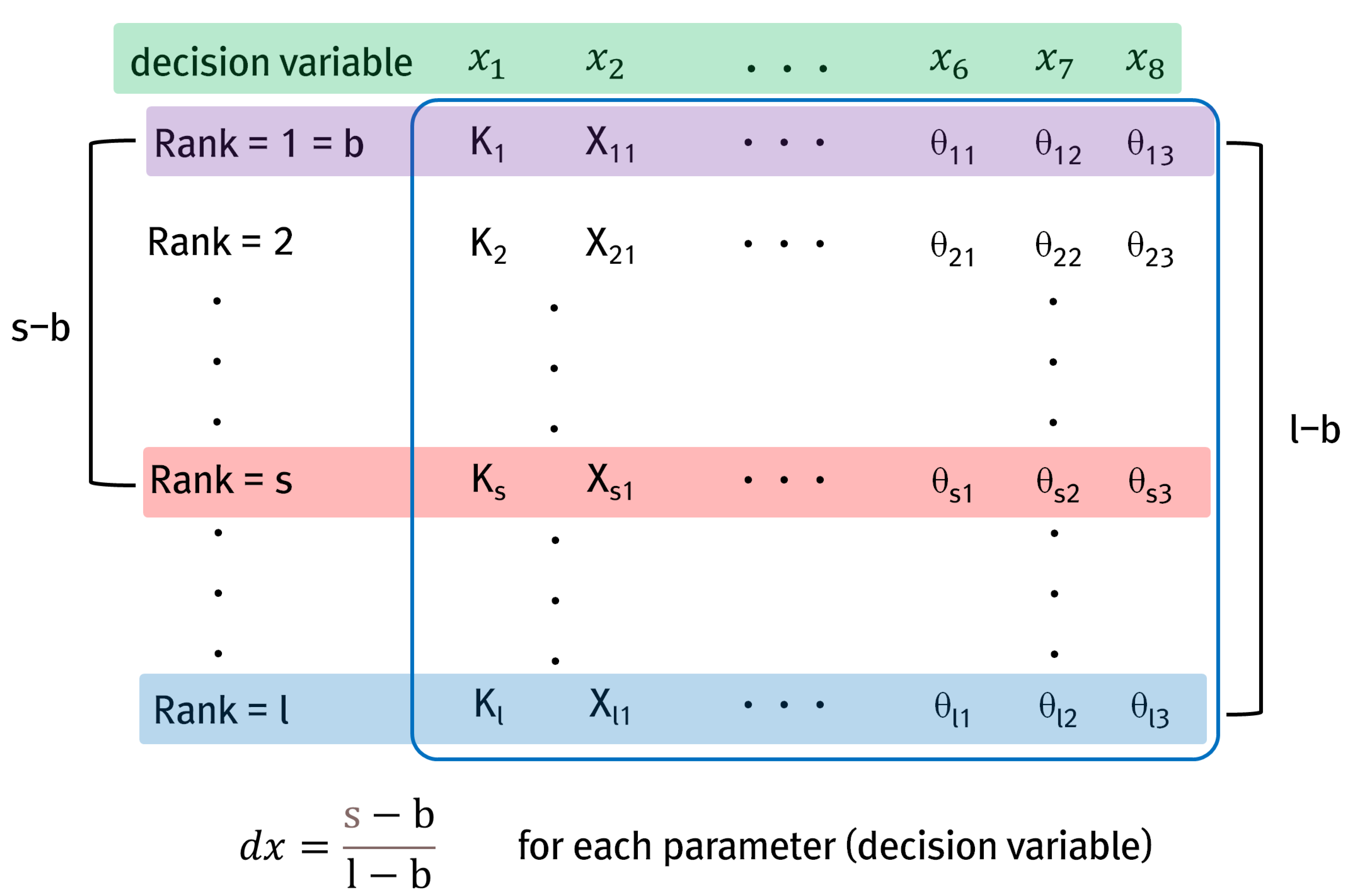
where MTF is the calculated modulation transfer function value. The term random(−1, 1) is a random value between −1 and 1. In addition, CF is a parameter for lens compression. The calculation of MTF is based on the distance (dx) between the current best decision variable and the selected decision variable. dx can be calculated using Equation (27).
where dx is the relative distance between each decision variable, rank(xs) is the fitness rank of the selected decision variable (xs), rank(xb) is the fitness rank of the best decision variable (xb), and rank(xl) is the fitness rank of the worst decision variable (xl). The fitness rank is the order in which the values of the objective function are sorted. The worst decision variable has the lowest fitness rank. Figure 1 shows the relative distance of dx.
The calculation of the MTF by applying dx is shown in Equation (28).
where MTFs is the MTF value of the selected decision variable, and k is the total number of decision variables. In addition, dxs is the relative distance of the selected decision variable, and dxi is the relative distance of the i-th decision variable. The CF in SAVCA can be calculated as shown in Equation (29).
where xi is the i-th decision variable. The probability of applying the astigmatism correction process is determined using the AR. The new decision variable adjusted by the application of the astigmatism correction process on a local search is shown in Equation (30).
where AF is the angle of the astigmatic axis. The application process of SAVCA is summarized as follows: (1) generation of an initial solution group, (2) calculation of the fitness of the initial solution groups, (3) generation of a new solution, (4) application of MR and AR, (5) decision to replace after comparing the new solution with the worst solution in the existing solution group, and (6) repeating (2)–(5) until the total number of iterations is reached. The worst solution is the solution with the lowest fitness rank among the existing solution group. Figure 2 shows the application process.
An initial solution group was created to apply SAVCA to the new Muskingum flood routing model. The weighted inflow, storage, outflow, and SSQ were then calculated. According to the probability of DR1, a new solution was generated by a global search, or one of the existing solution groups was selected through a local search. When creating a new solution with a global search, a new decision variable was created in the positive and negative directions based on the current best decision variable. Each new decision variable was corrected using the MR and AR. In addition, the weighted inflow, storage, outflow, and SSQ were calculated using the new solution with new decision variables. Whether a new solution should be added to the existing solution group was determined by comparing the SSQ of the new solution with the SSQ of the worst solution among the existing group of solutions.
2.4. Flood Data
Five types of flood data were applied to the Muskingum flood routing models: Wilson’s flood data, Wang’s flood data, flood data for River Wye December in 1960, Sutculer flood data, and flood data for River Wyre October in 1982 [5,39,40,41]. All flood data used in this study have been applied in several Muskingum flood routing models in existing studies. The most important aspect of the Muskingum flood routing model is the range of each parameter. The range of each parameter in the new Muskingum flood routing model applied to the five flood datasets is presented in Table 2.
Various Muskingum flood routing models, i.e., LMM, LMM-L, NLMM, NLMM-L, ANLMM-L, and the new Muskingum flood routing model, were compared herein. The parameters used in each Muskingum flood routing model are listed in Table 3.
Differences were observed in the results of the Muskingum flood routing models proposed in other studies. However, the simulation used in this study was conducted according to the parameters listed in Table 3. The data values from existing studies were considered only up to two decimal points when using them as an input for the models in this study. The parameters of Muskingum flood routing models without results from previous studies were obtained by applying SAVCA. However, the values of each parameter were all calculated differently.
3. Application and Results
The first flood dataset used for the application of all Muskingum flood routing models was Wilson’s flood data. The parameters of the LMM for Wilson’s flood data were determined to be 29.164640 for K, and 0.118200 for X1. The parameters of the new Muskingum flood routing model for Wilson’s flood data were determined to be 0.943442 for K, 0.340333 for X1, −0.00102 for X2, 1.744439 for m, −0.02166 for β, 0.758873 for θ1, 0.230779 for θ2, and 0.047773 for θ3. The results, including those obtained using the new Muskingum flood routing model, are compared in Table 4.
Among the results in Table 4, those of the LMM-L, NLMM, NLMM-L, and ANLMM-L were calculated in previous studies [2,5,9,42]. The results of LMM and new Muskingum flood routing model were calculated using Wilson’s flood data by applying SAVCA. Notably, the results of the LMM are better than those of the LMM-L. This is because the results of the LMM-L are the results of a previous study wherein the optimization method was not used, while the results of the LMM were obtained using SAVCA. It should be noted that the results of the new Muskingum flood routing model were better than those of the LMM, LMM-L, NLMM, NLMM-L, and ANLMM-L because the new Muskingum flood routing model showed the smallest error in the initial part from 0 to 24 h and showed the smallest error in the overall results. Because the errors of the NLMM-L and ANLMM-L were small, the new Muskingum flood routing model did not lead to a substantial improvement.
Among the existing Muskingum flood routing models, ANLMM-L showed the best results (smallest error). The difference in SSQ between the ANLMM-L and new Muskingum flood routing model was 0.43 (m3/s)2. The differences between the results of the two models were most notable from 6 to 18 h and from 108 to 126 h. The new Muskingum flood routing model showed the closest outflow to the observed outflow from 6 to 18 h. Among other Muskingum flood routing models, the outflows obtained from LMM-L at 6 h, LMM at 12 h, and NLMM-L at 18 h were close to the observed outflow. The difference between the observed outflow and the outflow obtained from the new Muskingum flood routing model was smaller than that attained using other Muskingum flood routing models.
The second flood dataset was Wang’s flood data. The parameters of the LMM-L for Wang’s flood data were determined to be 1.075331 for K, −0.762101 for X1, and −0.003024 for β. The parameters of the new Muskingum flood routing model for Wang’s flood data were determined to be 0.079266 for K, −1.49742 for X1, 0.011592 for X2, 1.360300 for m, −0.000450 for β, 0.421275 for θ1, 0.044483 for θ2, and 0.261537 for θ3. The results using Wang’s flood data, including those for the new Muskingum flood routing model, are compared in Table 5.
The results of LMM, NLMM, NLMM-L, and ANLMM-L were calculated in previous studies [2,8,9,39]. The results of LMM-L and new Muskingum flood routing model were calculated by applying SAVCA. Notably, the results improved dramatically when the lateral inflow was considered, indicated by the difference between the results of the LMM and LMM-L and between those of the NLMM and NLMM-L. A difference between the results of the ANLMM-L and new Muskingum flood routing model was also observed, although it was not due to a lateral inflow but to differences in the calculation equations of the weighted inflow and storage. The results of the new Muskingum flood routing model were overwhelmingly better than those of other Muskingum flood routing models because the new Muskingum flood routing model showed the smallest error in the latter part from 19 to 29 h and showed the smallest error in the overall results.
Among the existing Muskingum flood routing models, the ANLMM-L showed the best results (smallest error). The difference in SSQ between the ANLMM-L and new Muskingum flood routing model was 149.56 (m3/s)2. The difference between the two results was clear from 228 (19) to 288 (24) h. The differences in the outflow obtained using the Muskingum flood routing models and the observed outflow was small. The outflow calculated by the new Muskingum flood routing model was closest to the observed outflow. Among other Muskingum flood routing models, the outflow obtained using NLMM at 21 h was close to the observed outflow. The difference between the observed outflow and the outflow obtained using the new Muskingum flood routing model was smaller than that when using other Muskingum flood routing models.
The third flood dataset was the flood data of River Wye December in 1960. The parameters for the LMM using these data were determined to be 23.877307 for K, and 0.153174 for X1. The parameters for the new Muskingum flood routing model using these data were determined to be 2.318963 for K, 0.499999 for X1, 0.000390 for X2, 1.359406 for m, 0.057839 for β, 0.805567 for θ1, 0.233550 for θ2, and 6.88×10⁻¹¹ for θ3. The results of all the models for these data are compared in Table 6.
LMM-L, NLMM, NLMM-L, and ANLMM-L results were calculated in previous studies [2,5,9,42]. The results of LMM and new Muskingum flood routing model were calculated by applying SAVCA. Table 6 displays a notable difference between the results of the LMMs and NLMMs; the difference was large because the error in the flood data of River Wye from December 1960 was large. The new Muskingum flood routing model results were better than those of other Muskingum flood routing models because the new Muskingum flood routing model showed the smallest error from 102 to 198 h including the peak value and showed the smallest error in the overall result.
Among other Muskingum flood routing models, ANLMM-L showed the best results (smallest error). The difference in SSQ between the ANLMM-L and new Muskingum flood routing model was 1677.99 (m3/s)2. The greatest difference between the models occurred at 138–186 h. Among other Muskingum flood routing models, the outflow from ANLMM-L was close to the observed outflow at 180 and 186 h. The difference between the observed outflow and the outflow for the new Muskingum flood routing model was smaller than that for other Muskingum flood routing models.
The fourth flood dataset used was Sutculer flood data which is a flood data with a double-peak. The parameters of the LMM for Sutculer flood data were determined to be 1.0 for K, and −0.006097 for X1. The parameters of the LMM-L for Sutculer flood data were determined to be 1.0 for K, −0.025914 for X1, and −0.041042 for β. The parameters of the NLMM for Sutculer flood data were determined to be 1.0 for K, −0.053787 for X1, and 1.002498 for m. The parameters of the new Muskingum flood routing model for Sutculer flood data were determined to be 0.931599 for K, −0.092988 for X1, 0.009066 for X2, 1.000013 for m, −0.036144 for β, 0.817639 for θ1, 0.214801 for θ2, and 0.745272 for θ3. The results of all models are shown in Table 7.
Among the results in Table 7, those of NLMM-L and ANLMM-L were calculated in previous studies [2,9]. The results of LMM, LMM-L, NLMM, and new Muskingum flood routing model were calculated by applying the SAVCA. Notably, the models that consider the lateral inflow show good results. In addition, the results of LMM-L, NLMM-L, and ANLMM-L were better than those of LMM and NLMM because LMM-L, NLMM-L, and ANLMM-L showed relatively small errors in the overall results. Moreover, the difference between the results of the new Muskingum flood routing model and other Muskingum flood routing models was substantial.
The ANLMM-L showed the best results (smallest error) among the considered models. The difference in SSQ between the ANLMM-L and new Muskingum flood routing model was 63.22 (m3/s)2. The time required to show the difference between the two results ranged from 1 to 3 h. At 1 h, the outflow of most Muskingum flood routing models was close to the observed outflow. At 2 and 3 h, except for the new Muskingum flood routing model, the outflow of most Muskingum flood routing models showed a difference from the observed outflow.
The last flood dataset analyzed was the flood data of River Wyre October in 1982. The parameters of the LMM for the flood data of River Wyre from October 1982 were determined to be 3.950351 for K and 0.295668 for X1. The parameters of the NLMM for the flood data of River Wyre from October 1982 were determined to be 8.248204 for K, 0.284338 for X1, and 0.812821 for m. The parameters of the new Muskingum flood routing model for the flood data of River Wyre from October 1982 were determined to be 0.931599 for K, −0.092988 for X1, 0.009066 for X2, 1.000013 for m, −0.036144 for β, 0.817639 for θ1, 0.214801 for θ2, and 0.745272 for θ3; the results, and their comparison with those of the other models, are shown in Table 8.
Of the results given in Table 8, the LMM-L, NLMM-L, and ANLMM-L results were calculated in previous studies [2,5,9], while those of the LMM and NLMM were calculated by applying SAVCA; the results of the latter two models were the same. The errors were the greatest for the results of both LMM and NLMM, and some of the calculated outflow values obtained were negative. The new Muskingum flood routing model results in Table 8 were also calculated by applying SAVCA.
Notably, the results obtained for the models considering the lateral inflow were good; those of the LMM-L, NLMM-L, and ANLMM-L were significantly better than those of the LMM and NLMM. The difference in the results of all Muskingum flood routing models occurs from 26 to 31 h. The outflows of NLMM-L, ANLMM-L, and new Muskingum flood routing model were the closest to the observed outflow from 26 to 31 h. Although the results of the NLMM-L and ANLMM-L were similar to the observed outflow at 26 h, these differed over time. However, the new Muskingum flood routing model results did not differ significantly from the observed outflow from 26 to 31 h. ANLMM-L showed the best results (smallest error) among the existing Muskingum flood routing models. The difference in SSQ between the ANLMM-L and new Muskingum flood routing model was 1.35 (m3/s)2. Although varying results were obtained when using different flood data for the various models, the overall results of new Muskingum flood routing model were better than those of other Muskingum flood routing models because the error of new Muskingum flood routing model was relatively small in the latter part from 16 to 31 h.
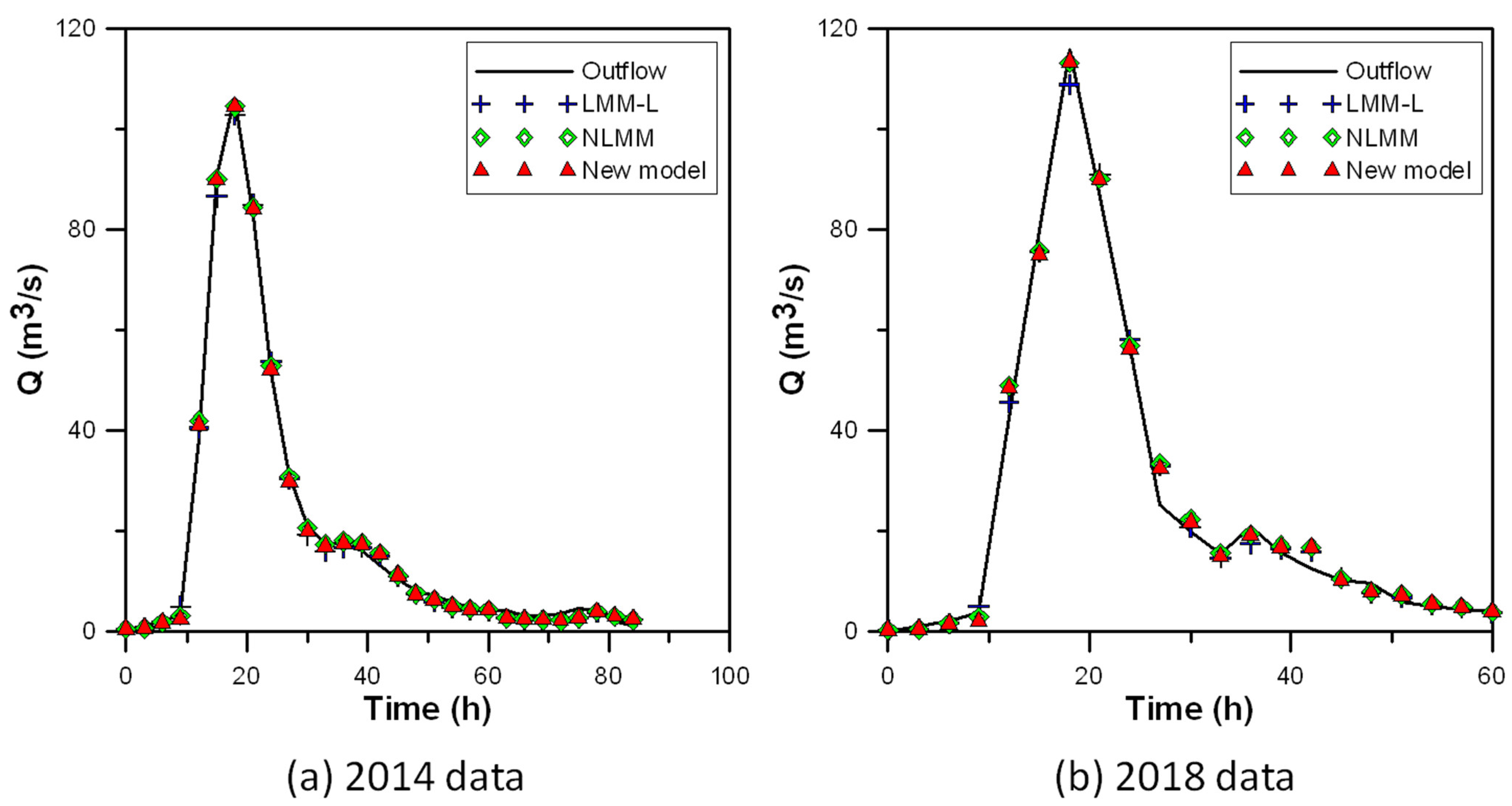
The new flood data in Daechung were applied to calibrate and validate the new Muskingum flood routing model. The flood data in April, 2014 were used for calibration and the flood data in April, 2018 were used for validation. Among various Muskingum flood routing models, LMM-L considering lateral inflow to LMM, NLMM considering nonlinearity to LMM and new Muskingum flood routing model were applied to Daechung flood data and compared.
The parameters of LMM were 3.989981 for K and −0.034950 for X. The parameters of LMM-L were 3.865970 for K, −0.043293 for X, and −0.020080 for β. The parameters of NLMM were 2.225924 for K, −1.5 for X, and 1.0 for m. The parameters of NLMM-L were 2.225076 for K, −1.406061 for X, 1.000000 for m, −0.007072 for β, 1.000000 for θ. The parameters of ANLMM-L were 2.123526 for K, −1.500000 for X, 1.000000 for m, −0.010223 for β, 1.000000 for θ1, and 0.017871 for θ2. The parameters of new Muskingum flood routing model were 2.220910 for K, −1.498329 for X1, 0.094832 for X2, 1.000008 for m, −0.012616 for β, 0.999660 for θ1, 0.000093 for θ2, and 0.000288 for θ3. Each parameter was applied equally for 2014 and 2018 data. A total of 100 simulations were conducted for each Muskingum flood routing model, yielding the best results. Table 9 shows the results of Daechung flood data in 2014.
Based on the variable values determined from the 2014 flood data, it was applied to the 2018 flood data. Table 10 shows the results of Daechung flood data in 2018.
Figure 3 shows the results of calibration and validation in Daechung flood data.
In the 2014 flood data, the SSQs of LMM, LMM-L, NLMM, NLMM-L, ANLMM-L and new Muskingum flood routing model were 88.23, 73.81, 43.79, 42.32, 40.16, and 39.55, respectively. In the 2014 flood data, the error of new Muskingum flood routing model was relatively small and the calibration of new Muskingum flood routing model was relatively accurate. The SSQs of new Muskingum flood routing model in the 2018 flood data was relatively small. In the 2018 flood data, the SSQs of LMM, LMM-L, NLMM, NLMM-L, ANLMM-L and new Muskingum flood routing model were 221.92, 180.41, 171.45, 161.99, 159.84, and 157.64, respectively. In the results of Figure 2, more accurate flood routing was performed by applying the new Muskingum flood routing model compared to LMM, LMM-L, NLMM, NLMM-L and ANLMM-L.
4. Discussion
Because the calculation process differs for each Muskingum flood routing model, the time required to find the parameters when applying a meta-heuristic optimization algorithm is different for each method. The time required to apply SAVCA was summarized to determine the parameters of each Muskingum flood routing model for Wilson’s flood data. The parameters of SAVCA were set at a constant, and the simulation was conducted 10 times. In addition, the number of iterations was set to 100,000. Table 11 shows the time taken for SAVCA when using Wilson’s flood data.
Depending on the parameters of the SAVCA and flood data, the results over time using the Muskingum flood routing models differ from the results in Table 9. As the number of parameters of the Muskingum flood routing models increased, the time required also increased. The time required by LMMs, LMM and LMM-L, was the shortest. NLMM and NLMM-L required a greater amount of time compared to the LMMs. The new Muskingum flood routing model required more time than the ANLMM-L, which in turn required more time than the NLMM-L. The time required by the new Muskingum flood routing model was approximately 1.5-times that required by LMM and LMM-L. In conclusion, the new Muskingum flood routing model produced more accurate results but took more time owing to the greater number of parameters and calculations.
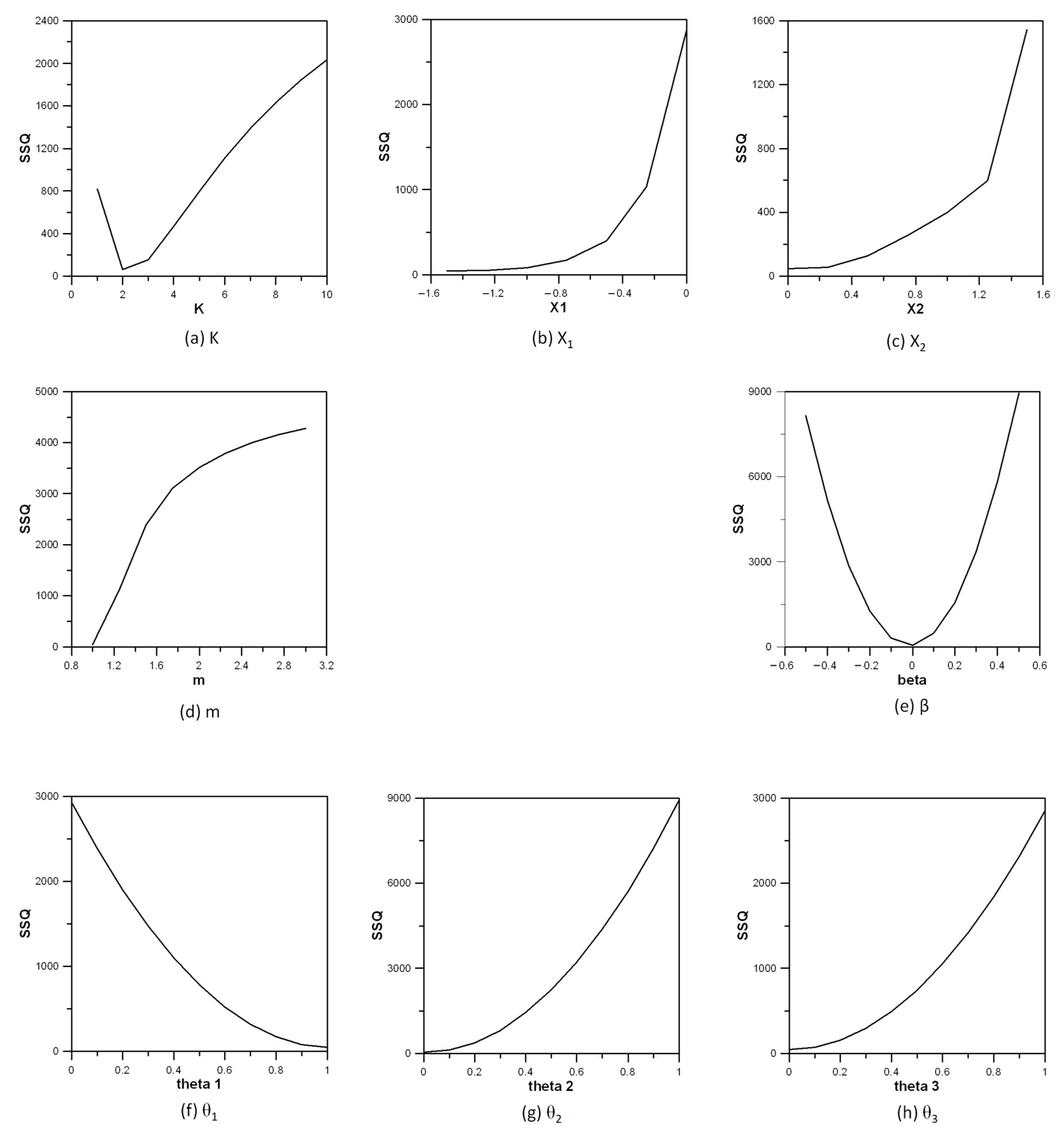
An analysis was conducted on how each parameter of new Muskingum flood routing model affects the results. Daechung flood data in April, 2014 was applied to analyze the sensitivity of each parameter in the new Muskingum flood routing model. Figure 4 showed the results of the sensitivity analysis for the parameters in the new Muskingum flood routing model.
SSQ decreases and then increases as parameter K increases, and SSQ increases as parameter X1 increases. SSQ increases as parameter X2 increases and SSQ increases as parameter m increases. SSQ decreases and then increases as parameter β increases, and SSQ decreases as the parameter θ1 increases. SSQ increases as parameter θ2 increases, and SSQ increases as parameter θ3 increases. As each parameter changed, the change of the results was not constant. It is difficult to find a uniform pattern in all the results. However, what can be confirmed from the results of sensitivity analysis is that a meta-heuristic optimization algorithm such as SAVCA is required to produce results with a low SSQ.
5. Conclusions
The Muskingum flood routing model is a representative hydrologic flood routing model that is widely used owing to its easy applicability. The proposed Muskingum flood routing model in this study is a simple model that can be applied by researchers that use the existing Muskingum models for accurate flood routing.
In this study, the new Muskingum flood routing model was applied to various flood data, and the results obtained were compared with those of previously developed Muskingum flood routing models. As an index for comparison, the error was calculated between the observed and simulated outflows using the SSQ, NSE and RMSE. In addition, SAVCA, a meta-heuristic optimization algorithm, was applied to adjust the parameters of the new Muskingum flood routing model.
In the sensitivity analysis, the changes of the eight parameters in the new Muskingum flood routing model are different. There are parameters whose results are improved as the value (θ1) increases, some parameters (m, θ2, θ3, x1, x2) whose results are improved as the value decreases, and some parameters (K, β) whose results are changed (improved and then deteriorated) as the value increases. The eight parameters of the new Muskingum flood routing model are decision variables of SAVCA and are calculated through the optimization process.
Muskingum flood routing models considering the lateral inflow are capable of relatively sophisticated simulations, which corroborates that the influence of lateral inflow on the outflow can be considered. Among the existing models, the ANLMM-L showed the highest accuracy, although the difference between its results and those of the other Muskingum flood routing models was insignificant. In the new Muskingum flood routing model, the improved calculation method of the inflow at previous time and next time reflected the trend of the observed outflow.
Since the Muskingum flood routing model proposed in this study has eight parameters, the calculation process is more complicated than the existing Muskingum flood routing models. Accurate flood prediction is possible due to the complicated calculation process, but the calculation time is long.
Many studies, including this study, have been performed by applying various meta-heuristic optimization algorithms to the Muskingum flood routing models. Since various optimization algorithms cannot show advantages in all problems, the results can be improved by appropriately selecting the operators of each meta-heuristic optimization algorithm. In addition, deep learning techniques have been widely used to apply various flood prediction methods including Muskingum flood routing models. By replacing the optimizer in deep learning techniques with meta-heuristic optimization algorithms, it would be possible to produce improved results in flood prediction.
Funding
This research was funded by the National Research Foundation (NRF) of Korea (NRF-2019R1I1A3A01059929).
Institutional Review Board Statement
Not applicable.
Informed Consent Statement
Not applicable.
Acknowledgments
This work was supported by a grant from The National Research Foundation (NRF) of Korea (NRF-2019R1I1A3A01059929).
Conflicts of Interest
The author declares no conflict of interest.
Abbreviations
| ANLMM-L | Advanced nonlinear Muskingum flood routing model considering continuous inflow |
| NLMM-L | Nonlinear Muskingum flood routing model incorporating lateral flow |
| NLMM | Nonlinear Muskingum method |
| LMM-L | Linear Muskingum method incorporating lateral flow |
| LMM | Linear Muskingum method |
| SAVCA | Self-adaptive vision correction algorithm |
| DR1 | Division rate 1 |
| DR2 | Division rate 2 |
| MTF | Modulation transfer function |
| CF | Compression factor |
| AR | Astigmatic rate |
| AF | Astigmatic angle |
| SSQ | Sum of squares |
| NSE | Nash–Sutcliffe efficiency |
| RMSE | Root mean square error |
References
- Go, I.H. Development of watershed integrated water resource management technique. J. Korea Water Resour. Assoc. 2004, 37, 10–15. [Google Scholar]
- Lee, E.H.; Lee, H.M.; Kim, J.H. Development and application of advanced Muskingum flood routing model considering continuous flow. Water 2018, 10, 760. [Google Scholar] [CrossRef] [Green Version]
- Absi, R. Reinvestigating the parabolic-shaped eddy viscosity profile for free surface flows. Hydrology 2021, 8, 126. [Google Scholar] [CrossRef]
- McCarthy, G.T. The unit hydrograph and flood routing. In Proceedings of Conference of North Atlantic Division; U.S. Army Corps of Engineers: New London, CT, USA, 1938. [Google Scholar]
- O’donnell, T. A direct three-parameter Muskingum procedure incorporating lateral inflow. Hydrol. Sci. J. 1985, 30, 479–496. [Google Scholar] [CrossRef] [Green Version]
- Tung, Y.K. River flood routing by nonlinear Muskingum method. J. Hydraul. Eng. 1985, 111, 1447–1460. [Google Scholar] [CrossRef] [Green Version]
- Das, A. Parameter estimation for Muskingum models. J. Irrig. Drain. Eng. 2004, 130, 140–147. [Google Scholar] [CrossRef]
- Geem, Z.W. Parameter estimation for the nonlinear Muskingum model using the BFGS technique. J. Irrig. Drain. Eng. 2006, 132, 474–478. [Google Scholar] [CrossRef]
- Karahan, H.; Gurarslan, G.; Geem, Z.W. A new nonlinear Muskingum flood routing model incorporating lateral flow. Eng. Optim. 2015, 47, 737–749. [Google Scholar] [CrossRef]
- Bozorg-Haddad, O.; Abdi-Dehkordi, M.; Hamedi, F.; Pazoki, M.; Loáiciga, H.A. Generalized storage equations for flood routing with nonlinear Muskingum models. Water Resour. Manag. 2019, 33, 2677–2691. [Google Scholar] [CrossRef]
- Gill, M.A. Flood routing by the Muskingum method. J. Hydrol. 1978, 36, 353–363. [Google Scholar] [CrossRef]
- Yoon, J.; Padmanabhan, G. Parameter estimation of linear and nonlinear Muskingum models. J. Water Resour. Plann. Manag. 1993, 119, 600–610. [Google Scholar] [CrossRef]
- Mohan, S. Parameter estimation of nonlinear Muskingum models using genetic algorithm. J. Hydraul. Eng. 1997, 123, 137–142. [Google Scholar] [CrossRef]
- Luo, J.; Xie, J. Parameter estimation for nonlinear Muskingum model based on immune clonal selection algorithm. J. Hydrol. Eng. 2010, 15, 844–851. [Google Scholar] [CrossRef]
- Barati, R. Parameter estimation of nonlinear Muskingum models using Nelder-Mead simplex algorithm. J. Hydrol. Eng. 2011, 16, 946–954. [Google Scholar] [CrossRef]
- Orouji, H.; Bozorg Haddad, O.; Fallah-Mehdipour, E.; Marino, M.A. Estimation of Muskingum parameter by meta-heuristic algorithms. In Proceedings of the Institution of Civil Engineers-Water Management; Thomas Telford Ltd.: London, UK, 2013; Volume 166, pp. 315–324. [Google Scholar]
- Niazkar, M.; Afzali, S.H. Assessment of modified honey bee mating optimization for parameter estimation of nonlinear Muskingum models. J. Hydrol. Eng. 2015, 20, 04014055. [Google Scholar] [CrossRef]
- Kang, L.; Zhang, S. Application of the elitist-mutated PSO and an improved GSA to estimate parameters of linear and nonlinear Muskingum flood routing models. PLoS ONE 2017, 11, e0147338. [Google Scholar] [CrossRef]
- Moghaddam, A.; Behmanesh, J.; Farsijani, A. Parameters estimation for the new four-parameter nonlinear Muskingum model using the particle swarm optimization. Water Resour. Manag. 2016, 30, 2143–2160. [Google Scholar] [CrossRef]
- Hamedi, F.; Bozorg-Haddad, O.; Pazoki, M.; Asgari, H.R.; Parsa, M.; Loáiciga, H.A. Parameter estimation of extended nonlinear Muskingum models with the weed optimization algorithm. J. Irrig. Drain. Eng. 2016, 142, 04016059. [Google Scholar] [CrossRef]
- Perumal, M.; Tayfur, G.; Rao, C.M.; Gurarslan, G. Evaluation of a physically based quasi-linear and a conceptually based nonlinear Muskingum methods. J. Hydrol. 2017, 546, 437–449. [Google Scholar] [CrossRef]
- Zhang, S.; Kang, L.; Zhou, B. Parameter estimation of nonlinear Muskingum model with variable exponent using adaptive genetic algorithm. In Environmental Conservation, Clean Water, Air & Soil (CleanWAS); IWA Publishing: London, UK, 2017; pp. 231–237. [Google Scholar]
- Bagatur, T.; Onen, F. Development of predictive model for flood routing using genetic expression programming. J. Flood Risk Manag. 2018, 11, S444–S454. [Google Scholar] [CrossRef] [Green Version]
- Akbarifard, S.; Qaderi, K.; Alinnejad, M. Parameter estimation of the nonlinear Muskingum flood-routing model using water cycle algorithm. J. Watershed Manag. Res. 2018, 8, 34–43. [Google Scholar] [CrossRef]
- Talatahari, S.; Sheikholeslami, R.; Farahmand Azar, B.; Daneshpajouh, H. Optimal parameter estimation for Muskingum model using a CSS-PSO method. Adv. Mech. Eng. 2013, 5, 480954. [Google Scholar] [CrossRef]
- Ouyang, A.; Li, K.; Truong, T.K.; Sallam, A.; Sha, E.H.M. Hybrid particle swarm optimization for parameter estimation of Muskingum model. Neural Comput. Appl. 2014, 25, 1785–1799. [Google Scholar] [CrossRef]
- Haddad, O.B.; Hamedi, F.; Fallah-Mehdipour, E.; Orouji, H.; Marino, M.A. Application of a hybrid optimization method in Muskingum parameter estimation. J. Irrig. Drain. Eng. 2015, 141, 04015026. [Google Scholar] [CrossRef] [Green Version]
- Kang, L.; Zhou, L.; Zhang, S. Parameter estimation of two improved nonlinear Muskingum models considering the lateral flow using a hybrid algorithm. Water Resour. Manag. 2017, 31, 4449–4467. [Google Scholar] [CrossRef]
- Ehteram, M.; Binti Othman, F.; Mundher Yaseen, Z.; Abdulmohsin Afan, H.; Falah Allawi, M.; Najah Ahmed, A.; Shaid, S.; Singh, V.; El-Shafie, A. Improving the Muskingum flood routing method using a hybrid of particle swarm optimization and bat algorithm. Water 2018, 10, 807. [Google Scholar] [CrossRef] [Green Version]
- O’Sullivan, J.J.; Ahilan, S.; Bruen, M. A modified Muskingum routing approach for floodplain flows: Theory and practice. J. Hydrol. 2012, 470, 239–254. [Google Scholar] [CrossRef] [Green Version]
- Easa, S.M. New and improved four-parameter non-linear Muskingum model. In Proceedings of the Institution of Civil Engineers-Water Management; Thomas Telford Ltd.: London, UK, 2014; Volume 167, pp. 288–298. [Google Scholar]
- Yoo, C.; Lee, J.; Lee, M. Parameter estimation of the Muskingum channel flood-routing model in ungauged channel reaches. J. Hydrol. Eng. 2017, 22, 05017005. [Google Scholar] [CrossRef]
- Karahan, H.; Gurarslan, G.; Geem, Z.W. Parameter estimation of the nonlinear Muskingum flood-routing model using a hybrid harmony search algorithm. J. Hydrol. Eng. 2013, 18, 352–360. [Google Scholar] [CrossRef]
- Niazkar, M.; Afzali, S.H. Application of new hybrid optimization technique for parameter estimation of new improved version of Muskingum model. Water Resour. Manag. 2016, 30, 4713–4730. [Google Scholar] [CrossRef]
- Niazkar, M.; Afzali, S.H. Parameter estimation of an improved nonlinear Muskingum model using a new hybrid method. Hydrol. Res. 2017, 48, 1253–1267. [Google Scholar] [CrossRef]
- Lee, E.H. Application of self-adaptive vision-correction algorithm for water-distribution problem. KSCE J. Civ. Eng. 2021, 25, 1106–1115. [Google Scholar] [CrossRef]
- Kim, Y.N. Development of Exponential Bandwidth Harmony Search with Centralized Global Search. Master’s Thesis, Chungbuk National University, Cheongju, Korea, 2021. (In Korean). [Google Scholar]
- Chow, V.T. Open-Channel Hydraulics; McGraw-Hill Civil Engineering Series; McGraw-Hill: New York, NY, USA, 1959. [Google Scholar]
- Wang, W.; Xu, Z.; Qiu, L.; Xu, D. Hybrid chaotic genetic algorithms for optimal parameter estimation of Muskingum flood routing model. In Proceedings of the International Joint Conference on Computational Sciences and Optimization, Sanya, China, 24–26 April 2009; pp. 215–218. [Google Scholar]
- Bajracharya, K.; Barry, D.A. Accuracy criteria for linearised diffusion wave flood routing. J. Hydrol. 1997, 195, 200–217. [Google Scholar] [CrossRef]
- Ulke, A. Flood Routing Using Muskingum Method. Master’s Thesis, Suleyman Demirel University, Kaskelen, Kazakhstan, 2003. (In Turkish). [Google Scholar]
- Karahan, H.; Gurarslan, G. Modelling flood routing problems using kinematic wave approach: Sutculer example. In Proceedings of the 7th National Hydrology Congress, Isparta, Turkey, 26–27 September 2013. [Google Scholar]
Figure 1.
Relative distance of dx.

Figure 2.
Application process.
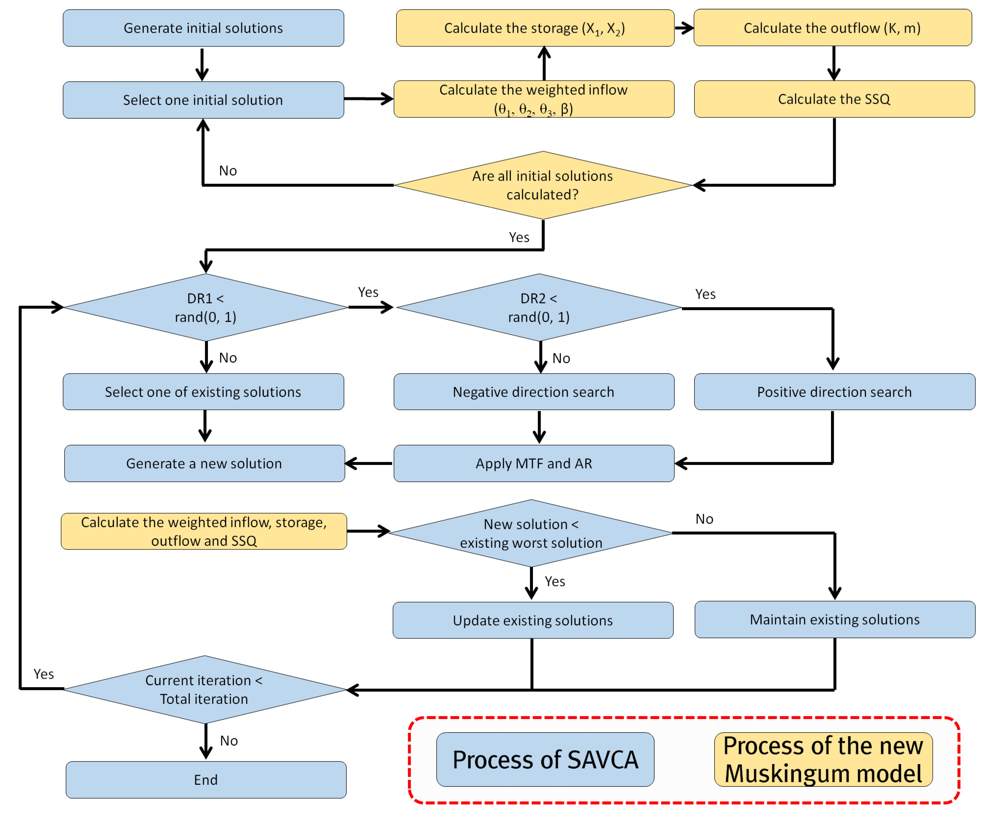
Figure 3.
Results of calibration and validation in Daechung flood data (a) 2014 flood data; (b) 2018 flood data..
Figure 3.
Results of calibration and validation in Daechung flood data (a) 2014 flood data; (b) 2018 flood data..

Figure 4.
Results of sensitivity analysis for the parameters in the new Muskingum flood routing model.
Figure 4.
Results of sensitivity analysis for the parameters in the new Muskingum flood routing model.


Table 1.
Parameter types of SAVCA.
| Parameters | DR1 | DR2 | MR | CF | AR | AF |
|---|---|---|---|---|---|---|
| Types | Self-adaptive | Self-adaptive | Fixed | Self-adaptive | Fixed | Fixed |
Table 2.
Range of parameters in the new Muskingum flood routing model.
| Parameters | Wilson’s Flood Data | Wang’s Flood Data | Flood Data for River Wye December in 1960 | Sutculer Flood Data | Flood Data for River Wyre October in 1982 |
|---|---|---|---|---|---|
| K | 0.01–50.00 | 0.01–50.00 | 0.01–50.00 | 0.01–50.00 | 0.01–50.00 |
| X1 | −0.50–0.50 | −1.50–1.50 | −0.50–0.50 | −0.50–0.50 | −0.50–0.50 |
| X2 | −0.50–0.50 | −1.50–1.50 | −0.50–0.50 | −0.50–0.50 | −0.50–0.50 |
| m | 1.00–3.00 | 1.00–3.00 | 1.00–3.00 | 1.00–3.00 | 0.00–1.00 |
| β | −0.10–0.10 | −3.00–3.00 | −0.10–0.10 | −0.10–0.10 | −3.00–3.00 |
| θ1 | 0.00–1.00 | 0.00–1.00 | 0.00–1.00 | 0.00–1.00 | 0.00–1.00 |
| θ2 | 0.00–1.00 | 0.00–1.00 | 0.00–1.00 | 0.00–1.00 | 0.00–1.00 |
| θ3 | 0.00–1.00 | 0.00–1.00 | 0.00–1.00 | 0.00–1.00 | 0.00–1.00 |
Table 3.
Parameters used in each Muskingum flood routing model (○: applied, X: not applied).
| Parameters | LMM | LMM-L | NLMM | NLMM-L | ANLMM-L | This Study |
|---|---|---|---|---|---|---|
| K | ○ | ○ | ○ | ○ | ○ | ○ |
| X1 | ○ | ○ | ○ | ○ | ○ | ○ |
| X2 | Ⅹ | Ⅹ | Ⅹ | Ⅹ | Ⅹ | ○ |
| m | Ⅹ | Ⅹ | ○ | ○ | ○ | ○ |
| β | Ⅹ | ○ | Ⅹ | ○ | ○ | ○ |
| θ1 | Ⅹ | Ⅹ | Ⅹ | ○ | ○ | ○ |
| θ2 | Ⅹ | Ⅹ | Ⅹ | Ⅹ | ○ | ○ |
| θ3 | Ⅹ | Ⅹ | Ⅹ | Ⅹ | Ⅹ | ○ |
Table 4.
Results when using Wilson’s flood data.
| Time (h) | Inflow (m3/s) | Outflow (m3/s) | LMM (m3/s) | LMM-L (m3/s) [5] | NLMM (m3/s) [42] | NLMM-L (m3/s) [9] | ANLMM-L (m3/s) [2] | This Study (m3/s) |
|---|---|---|---|---|---|---|---|---|
| 0 | 22 | 22 | 22.00 | 22.00 | 22.00 | 22.00 | 22.00 | 22.00 |
| 6 | 23 | 21 | 21.87 | 21.10 | 22.00 | 21.71 | 21.57 | 21.33 |
| 12 | 35 | 21 | 20.52 | 21.70 | 22.40 | 22.02 | 21.67 | 21.13 |
| 18 | 71 | 26 | 19.07 | 22.60 | 26.60 | 26.08 | 25.46 | 25.53 |
| 24 | 103 | 34 | 26.90 | 30.70 | 34.50 | 33.51 | 34.59 | 34.75 |
| 30 | 111 | 44 | 43.58 | 44.70 | 44.20 | 42.83 | 43.73 | 43.52 |
| 36 | 109 | 55 | 59.58 | 58.10 | 56.90 | 55.44 | 54.59 | 54.62 |
| 42 | 100 | 66 | 72.32 | 68.90 | 68.10 | 66.67 | 66.01 | 66.08 |
| 48 | 86 | 75 | 80.65 | 76.10 | 77.10 | 75.77 | 75.52 | 75.53 |
| 54 | 71 | 82 | 83.91 | 79.20 | 83.30 | 82.12 | 82.16 | 82.11 |
| 60 | 59 | 85 | 82.51 | 78.50 | 85.90 | 84.78 | 85.04 | 85.08 |
| 66 | 47 | 84 | 78.63 | 75.60 | 84.50 | 83.42 | 84.00 | 83.89 |
| 72 | 39 | 80 | 72.32 | 70.70 | 80.60 | 79.44 | 79.62 | 79.61 |
| 78 | 32 | 73 | 65.49 | 65.10 | 73.70 | 72.48 | 72.63 | 72.53 |
| 84 | 28 | 64 | 58.21 | 59.10 | 65.40 | 64.08 | 63.80 | 63.81 |
| 90 | 24 | 54 | 51.70 | 53.40 | 56.00 | 54.58 | 54.31 | 54.27 |
| 96 | 22 | 44 | 45.50 | 47.90 | 46.70 | 45.22 | 44.80 | 44.84 |
| 102 | 21 | 36 | 40.15 | 43.10 | 37.70 | 36.34 | 36.25 | 36.32 |
| 108 | 20 | 30 | 35.82 | 38.90 | 30.50 | 29.21 | 29.45 | 29.52 |
| 114 | 19 | 25 | 32.26 | 35.40 | 25.20 | 24.21 | 24.63 | 24.66 |
| 120 | 19 | 22 | 29.17 | 32.30 | 21.70 | 20.96 | 21.39 | 21.46 |
| 126 | 18 | 19 | 26.93 | 29.90 | 20.00 | 19.41 | 19.81 | 19.77 |
| SSQ (m3/s)2 | - | - | 605.63 | 815.68 | 36.77 | 9.82 | 4.54 | 4.11 |
| Squared root of SSQ (m3/s) | - | - | 24.61 | 28.56 | 6.06 | 3.13 | 2.13 | 2.03 |
| NSE | - | - | 0.974322 | 0.974326 | 0.992412 | 0.999583 | 0.999808 | 0.999826 |
| RMSE (m3/s) | - | - | 5.310259 | 5.369885 | 2.919411 | 0.683993 | 0.464124 | 0.442254 |
Table 5.
Results when using Wang’s flood data.
| Time (12 h) | Inflow (m3/s) | Outflow (m3/s) | LMM (m3/s) [39] | LMM-L (m3/s) | NLMM (m3/s) [8] | NLMM-L (m3/s) [9] | ANLMM-L (m3/s) [2] | This Study (m3/s) |
|---|---|---|---|---|---|---|---|---|
| 1 | 261 | 228 | 228.00 | 228.00 | 228.00 | 228.00 | 228.00 | 228.00 |
| 2 | 389 | 300 | 305.19 | 300.19 | 303.80 | 299.74 | 300.92 | 301.75 |
| 3 | 462 | 382 | 382.00 | 377.92 | 382.30 | 382.57 | 381.51 | 382.38 |
| 4 | 505 | 444 | 442.70 | 440.10 | 442.40 | 442.76 | 443.15 | 442.81 |
| 5 | 525 | 490 | 483.60 | 482.17 | 482.40 | 482.16 | 482.69 | 483.63 |
| 6 | 543 | 513 | 513.00 | 511.70 | 511.2 | 509.89 | 510.09 | 510.15 |
| 7 | 556 | 528 | 534.29 | 532.96 | 532.30 | 530.72 | 530.66 | 530.75 |
| 8 | 567 | 543 | 550.44 | 548.97 | 548.50 | 546.77 | 546.62 | 546.79 |
| 9 | 577 | 553 | 563.53 | 561.89 | 561.70 | 559.96 | 559.77 | 559.53 |
| 10 | 583 | 564 | 573.16 | 571.53 | 571.60 | 569.94 | 569.80 | 569.75 |
| 11 | 587 | 573 | 580.02 | 578.38 | 578.70 | 577.07 | 576.95 | 577.89 |
| 12 | 595 | 581 | 587.32 | 585.44 | 586.20 | 584.39 | 584.22 | 584.03 |
| 13 | 597 | 588 | 592.14 | 590.40 | 591.20 | 589.68 | 589.60 | 589.77 |
| 14 | 597 | 594 | 594.59 | 592.93 | 593.90 | 592.34 | 592.30 | 591.61 |
| 15 | 589 | 592 | 592.02 | 590.68 | 591.80 | 590.33 | 590.34 | 586.67 |
| 16 | 556 | 584 | 574.89 | 574.62 | 575.70 | 574.68 | 574.86 | 576.15 |
| 17 | 538 | 566 | 556.85 | 556.15 | 558.50 | 556.41 | 556.23 | 556.07 |
| 18 | 516 | 550 | 536.93 | 536.22 | 539.00 | 537.43 | 537.13 | 536.33 |
| 19 | 486 | 520 | 512.18 | 511.79 | 514.80 | 513.47 | 513.35 | 521.23 |
| 20 | 505 | 504 | 507.96 | 505.60 | 509.60 | 507.07 | 506.51 | 502.72 |
| 21 | 477 | 483 | 493.22 | 492.40 | 484.90 | 494.86 | 494.95 | 492.05 |
| 22 | 429 | 461 | 462.34 | 462.82 | 464.80 | 464.39 | 464.94 | 463.80 |
| 23 | 379 | 420 | 421.87 | 422.73 | 425.10 | 423.97 | 424.15 | 422.09 |
| 24 | 320 | 368 | 372.34 | 373.60 | 376.10 | 375.05 | 375.07 | 374.32 |
| 25 | 263 | 318 | 318.97 | 320.23 | 322.40 | 321.35 | 321.35 | 322.59 |
| 26 | 220 | 271 | 270.39 | 271.06 | 272.50 | 271.42 | 271.40 | 271.68 |
| 27 | 182 | 234 | 226.99 | 227.38 | 227.50 | 226.94 | 227.09 | 229.70 |
| 28 | 167 | 193 | 197.20 | 196.67 | 195.70 | 194.92 | 195.13 | 194.64 |
| 29 | 152 | 178 | 174.87 | 174.28 | 172.60 | 172.46 | 172.76 | 174.61 |
| SSQ (m3/s)2 | - | - | 1086.84 | 999.83 | 979.96 | 917.06 | 909.35 | 759.79 |
| Squared root of SSQ (m3/s) | - | - | 32.97 | 31.62 | 31.30 | 30.28 | 30.16 | 27.56 |
| NSE | - | - | 0.998247 | 0.998326 | 0.998359 | 0.998464 | 0.998478 | 0.998728 |
| RMSE (m3/s) | - | - | 6.008111 | 5.8711693 | 5.813054 | 5.623423 | 5.598762 | 5.118558 |
Table 6.
Results when using flood data of River Wye December in 1960.
| Time (h) | Inflow (m3/s) | Outflow (m3/s) | LMM (m3/s) | LMM-L (m3/s) [5] | NLMM (m3/s) [42] | NLMM-L (m3/s) [9] | ANLMM-L (m3/s) [2] | This Study (m3/s) |
|---|---|---|---|---|---|---|---|---|
| 0 | 154 | 102 | 102.00 | 102.00 | 102.00 | 102.00 | 102.00 | 102.00 |
| 6 | 150 | 140 | 118.15 | 116.00 | 154.00 | 149.50 | 146.52 | 141.89 |
| 12 | 219 | 169 | 115.12 | 120.00 | 152.00 | 156.59 | 155.74 | 155.50 |
| 18 | 182 | 190 | 152.64 | 147.00 | 181.00 | 191.40 | 194.41 | 185.46 |
| 24 | 182 | 209 | 161.35 | 158.00 | 191.00 | 200.79 | 194.19 | 190.53 |
| 30 | 192 | 218 | 165.67 | 165.00 | 185.00 | 195.14 | 196.05 | 195.99 |
| 36 | 165 | 210 | 178.37 | 176.00 | 187.00 | 197.46 | 198.35 | 196.69 |
| 42 | 150 | 194 | 177.11 | 178.00 | 179.00 | 188.48 | 186.83 | 188.20 |
| 48 | 128 | 172 | 173.05 | 176.00 | 162.00 | 170.80 | 172.12 | 175.53 |
| 54 | 168 | 149 | 152.45 | 164.00 | 141.00 | 148.10 | 150.37 | 157.72 |
| 60 | 260 | 136 | 140.42 | 160.00 | 154.00 | 162.59 | 167.56 | 169.06 |
| 66 | 471 | 228 | 137.74 | 167.00 | 198.00 | 210.36 | 216.61 | 213.24 |
| 72 | 717 | 303 | 192.13 | 218.00 | 264.00 | 281.58 | 294.27 | 287.51 |
| 78 | 1092 | 366 | 280.05 | 303.00 | 344.00 | 367.75 | 378.29 | 378.89 |
| 84 | 1145 | 456 | 511.40 | 484.00 | 416.00 | 447.65 | 461.17 | 465.87 |
| 90 | 600 | 615 | 797.99 | 690.00 | 599.00 | 629.57 | 612.03 | 609.41 |
| 96 | 365 | 830 | 781.75 | 700.00 | 871.00 | 892.78 | 862.51 | 863.65 |
| 102 | 277 | 969 | 674.00 | 642.00 | 834.00 | 859.01 | 884.60 | 887.00 |
| 108 | 227 | 665 | 565.24 | 572.00 | 689.00 | 719.30 | 737.54 | 730.86 |
| 114 | 187 | 519 | 472.11 | 505.00 | 535.00 | 567.50 | 565.33 | 555.56 |
| 120 | 161 | 444 | 392.21 | 442.00 | 397.00 | 427.85 | 414.97 | 410.06 |
| 126 | 143 | 321 | 326.86 | 386.00 | 283.00 | 308.86 | 297.45 | 300.33 |
| 132 | 126 | 208 | 275.37 | 338.00 | 202.00 | 220.90 | 216.14 | 224.40 |
| 138 | 115 | 176 | 233.04 | 296.00 | 152.00 | 163.64 | 164.43 | 174.61 |
| 144 | 102 | 148 | 200.36 | 260.00 | 124.00 | 131.90 | 134.94 | 143.56 |
| 150 | 93 | 125 | 172.80 | 228.00 | 106.00 | 111.93 | 114.46 | 121.64 |
| 156 | 88 | 114 | 150.03 | 201.00 | 94.00 | 99.28 | 101.24 | 106.75 |
| 162 | 82 | 106 | 132.71 | 179.00 | 88.00 | 92.90 | 94.00 | 97.42 |
| 168 | 76 | 97 | 118.75 | 160.00 | 82.00 | 86.14 | 86.94 | 89.67 |
| 174 | 73 | 89 | 106.60 | 144.00 | 75.00 | 79.34 | 80.13 | 82.79 |
| 180 | 70 | 81 | 97.18 | 130.00 | 73.00 | 76.46 | 76.87 | 78.56 |
| 186 | 67 | 76 | 89.65 | 118.00 | 69.00 | 73.13 | 73.54 | 74.88 |
| 192 | 63 | 71 | 83.66 | 109.00 | 66.00 | 69.85 | 70.23 | 71.46 |
| 198 | 59 | 66 | 78.25 | 100.00 | 62.00 | 65.09 | 65.60 | 67.24 |
| SSQ (m3/s)2 | - | - | 196,077.12 | 251,802.00 | 37,944.15 | 25,915.27 | 20,494.98 | 18,816.99 |
| Squared root of SSQ (m3/s) | - | - | 442.81 | 501.80 | 194.79 | 160.98 | 143.16 | 137.18 |
| NSE | - | - | 0.916666 | 0.921600 | 0.959208 | 0.988986 | 0.991290 | 0.992003 |
| RMSE (m3/s) | - | - | 77.082625 | 74.765750 | 53.930178 | 28.023612 | 24.921077 | 23.879109 |
Table 7.
Results when using Sutculer flood data.
| Time (h) | Inflow (m3/s) | Outflow (m3/s) | LMM (m3/s) | LMM-L (m3/s) | NLMM (m3/s) | NLMM-L (m3/s) [9] | ANLMM-L (m3/s) [2] | This Study (m3/s) |
|---|---|---|---|---|---|---|---|---|
| 0 | 7.53 | 7.00 | 7.00 | 7.00 | 7.00 | 7.00 | 7.00 | 7.00 |
| 1 | 9.06 | 8.00 | 7.59 | 7.25 | 7.58 | 7.24 | 7.26 | 8.14 |
| 2 | 28.00 | 23.00 | 10.06 | 9.11 | 9.94 | 9.00 | 9.01 | 11.97 |
| 3 | 79.80 | 25.00 | 29.95 | 27.66 | 29.56 | 27.35 | 27.35 | 25.63 |
| 4 | 64.30 | 75.00 | 76.04 | 74.92 | 75.86 | 74.84 | 74.81 | 73.93 |
| 5 | 38.20 | 60.00 | 63.47 | 61.36 | 63.70 | 61.57 | 61.59 | 62.61 |
| 6 | 41.40 | 40.00 | 39.84 | 37.33 | 39.96 | 37.40 | 37.41 | 37.54 |
| 7 | 41.30 | 41.00 | 41.30 | 39.64 | 41.31 | 39.63 | 39.62 | 39.37 |
| 8 | 33.80 | 41.00 | 40.87 | 39.42 | 40.92 | 39.47 | 39.47 | 39.72 |
| 9 | 32.00 | 32.00 | 34.10 | 32.55 | 34.15 | 32.57 | 32.58 | 32.56 |
| 10 | 29.00 | 30.00 | 31.95 | 30.66 | 31.98 | 30.68 | 30.68 | 31.10 |
| 11 | 35.00 | 34.00 | 29.51 | 28.03 | 29.49 | 28.00 | 28.00 | 29.48 |
| 12 | 63.10 | 35.00 | 36.30 | 34.10 | 36.10 | 33.93 | 33.93 | 36.09 |
| 13 | 110.00 | 60.00 | 64.26 | 60.98 | 63.81 | 60.62 | 60.62 | 63.47 |
| 14 | 170.00 | 105.00 | 110.82 | 105.81 | 110.12 | 105.25 | 105.25 | 108.08 |
| 15 | 216.00 | 160.00 | 169.24 | 162.69 | 168.46 | 162.06 | 162.07 | 157.14 |
| 16 | 131.00 | 206.00 | 208.43 | 203.95 | 208.54 | 204.11 | 204.11 | 205.42 |
| 17 | 101.00 | 128.00 | 133.73 | 126.88 | 134.55 | 127.58 | 127.61 | 126.32 |
| 18 | 65.00 | 97.00 | 100.81 | 96.74 | 101.33 | 97.14 | 97.10 | 98.08 |
| 19 | 62.40 | 61.00 | 66.91 | 63.14 | 67.19 | 63.33 | 63.32 | 63.18 |
| 20 | 53.80 | 60.00 | 62.16 | 59.71 | 62.26 | 59.78 | 59.76 | 59.18 |
| 21 | 36.30 | 50.00 | 53.27 | 51.37 | 53.44 | 51.51 | 51.50 | 51.71 |
| 22 | 29.60 | 33.00 | 36.89 | 35.07 | 37.03 | 35.16 | 35.16 | 35.19 |
| 23 | 25.00 | 27.00 | 29.75 | 28.44 | 29.82 | 28.49 | 28.48 | 28.49 |
| 24 | 21.30 | 23.00 | 25.06 | 24.00 | 25.11 | 24.03 | 24.03 | 24.13 |
| 25 | 19.60 | 19.00 | 21.42 | 20.47 | 21.44 | 20.49 | 20.49 | 20.53 |
| 26 | 18.00 | 18.00 | 19.61 | 18.80 | 19.63 | 18.81 | 18.81 | 18.90 |
| 27 | 17.30 | 17.00 | 18.05 | 17.28 | 18.06 | 17.29 | 17.29 | 17.38 |
| 28 | 17.00 | 17.00 | 17.33 | 16.60 | 17.33 | 16.60 | 16.60 | 16.63 |
| 29 | 16.00 | 17.00 | 16.96 | 16.29 | 16.97 | 16.29 | 16.29 | 16.53 |
| SSQ (m3/s)2 | - | - | 512.87 | 282.89 | 510.18 | 281.11 | 280.95 | 217.73 |
| Squared root of SSQ (m3/s) | - | - | 22.65 | 16.82 | 22.59 | 16.77 | 16.76 | 14.76 |
| NSE | - | - | 0.992557 | 0.995895 | 0.992596 | 0.995921 | 0.995922 | 0.996840 |
| RMSE (m3/s) | - | - | 4.134694 | 3.070802 | 4.123823 | 3.061080 | 3.060593 | 2.694028 |
Table 8.
Results when using flood data of River Wyre October in 1982.
| Time (h) | Inflow (m3/s) | Outflow (m3/s) | LMM (m3/s) | LMM-L (m3/s) [5] | NLMM (m3/s) | NLMM-L (m3/s) [9] | ANLMM-L (m3/s) [2] | This Study (m3/s) |
|---|---|---|---|---|---|---|---|---|
| 0 | 2.60 | 8.30 | 8.30 | 8.30 | 8.30 | 8.30 | 8.30 | 8.30 |
| 1 | 4.20 | 9.00 | 5.58 | 8.20 | 6.00 | 8.51 | 8.52 | 8.73 |
| 2 | 12.30 | 9.90 | 1.68 | 8.10 | 2.27 | 8.79 | 9.94 | 10.11 |
| 3 | 25.40 | 10.20 | 0.00 | 12.70 | 0.00 | 10.94 | 12.74 | 12.75 |
| 4 | 24.10 | 18.90 | 9.67 | 27.90 | 8.66 | 20.28 | 19.71 | 19.51 |
| 5 | 20.30 | 35.90 | 16.45 | 39.90 | 15.50 | 37.54 | 35.73 | 36.22 |
| 6 | 23.30 | 51.80 | 16.58 | 45.70 | 16.02 | 49.07 | 48.87 | 49.25 |
| 7 | 27.70 | 59.40 | 17.15 | 52.20 | 16.91 | 55.11 | 55.95 | 55.83 |
| 8 | 27.70 | 63.30 | 20.94 | 61.40 | 20.90 | 62.50 | 62.74 | 62.54 |
| 9 | 26.90 | 69.60 | 23.71 | 68.90 | 23.78 | 71.44 | 71.35 | 71.33 |
| 10 | 24.80 | 76.70 | 25.73 | 74.70 | 25.80 | 78.03 | 77.95 | 77.87 |
| 11 | 26.90 | 82.00 | 24.52 | 77.20 | 24.59 | 82.07 | 82.67 | 82.68 |
| 12 | 33.70 | 85.30 | 22.52 | 79.80 | 22.77 | 83.72 | 85.27 | 85.10 |
| 13 | 33.90 | 89.00 | 26.45 | 87.80 | 26.92 | 87.43 | 88.11 | 87.71 |
| 14 | 27.80 | 94.60 | 31.69 | 95.50 | 32.09 | 95.49 | 94.74 | 94.61 |
| 15 | 20.80 | 98.80 | 33.23 | 97.70 | 33.18 | 100.88 | 99.90 | 99.91 |
| 16 | 15.60 | 98.00 | 30.95 | 94.40 | 30.43 | 99.29 | 98.87 | 98.75 |
| 17 | 11.90 | 91.80 | 26.98 | 87.90 | 26.29 | 92.06 | 92.05 | 91.82 |
| 18 | 9.50 | 82.30 | 22.57 | 79.80 | 21.98 | 82.22 | 82.36 | 82.12 |
| 19 | 7.80 | 72.00 | 18.59 | 71.50 | 18.24 | 71.75 | 71.88 | 71.67 |
| 20 | 6.50 | 61.90 | 15.26 | 63.60 | 15.19 | 61.94 | 61.93 | 61.80 |
| 21 | 5.80 | 53.00 | 12.40 | 56.10 | 12.60 | 53.12 | 53.10 | 53.03 |
| 22 | 5.00 | 45.60 | 10.37 | 49.60 | 10.74 | 45.47 | 45.37 | 45.34 |
| 23 | 4.80 | 39.20 | 8.52 | 43.70 | 9.04 | 39.14 | 39.04 | 39.07 |
| 24 | 4.50 | 33.80 | 7.31 | 38.80 | 7.87 | 33.76 | 33.65 | 33.68 |
| 25 | 4.10 | 29.30 | 6.47 | 34.60 | 7.03 | 29.55 | 29.39 | 29.44 |
| 26 | 3.70 | 26.20 | 5.78 | 30.90 | 6.34 | 26.12 | 25.96 | 26.02 |
| 27 | 3.40 | 23.50 | 5.16 | 27.70 | 5.71 | 23.20 | 23.08 | 23.14 |
| 28 | 3.20 | 21.20 | 4.61 | 24.80 | 5.14 | 20.67 | 20.59 | 20.64 |
| 29 | 2.90 | 19.20 | 4.23 | 22.30 | 4.73 | 18.52 | 18.44 | 18.48 |
| 30 | 2.80 | 17.70 | 3.79 | 20.10 | 4.27 | 16.71 | 16.68 | 16.72 |
| 31 | 2.60 | 16.40 | 3.52 | 18.20 | 3.96 | 15.12 | 15.09 | 15.23 |
| SSQ (m3/s)2 | - | - | 53,544.67 | 468.84 | 53,544.99 | 53.66 | 40.16 | 38.81 |
| Squared root of SSQ (m3/s) | - | - | 231.40 | 21.65 | 231.40 | 7.33 | 6.34 | 6.23 |
| NSE | - | - | −0.213958 | 0.989570 | −0.213965 | 0.998842 | 0.999090 | 0.999120 |
| RMSE (m3/s) | - | - | 40.905633 | 3.790780 | 40.905755 | 1.263563 | 1.120320 | 1.101288 |
Table 9.
Results of Daechung flood data in 2014.
| Time (h) | Inflow (m3/s) | Outflow (m3/s) | LMM (m3/s) | LMM-L (m3/s) | NLMM (m3/s) | NLMM-L (m3/s) | ANLMM-L (m3/s) | This Study (m3/s) |
|---|---|---|---|---|---|---|---|---|
| 0 | 0.79 | 0.47 | 0.47 | 0.47 | 0.47 | 0.47 | 0.47 | 0.47 |
| 3 | 2.12 | 1.04 | 0.75 | 0.75 | 0.64 | 0.65 | 0.65 | 0.62 |
| 6 | 3.54 | 2.11 | 1.79 | 1.80 | 1.81 | 1.80 | 1.78 | 1.79 |
| 9 | 50.75 | 3.19 | 4.66 | 4.96 | 3.14 | 3.12 | 2.62 | 2.34 |
| 12 | 103.90 | 38.32 | 39.94 | 40.42 | 41.86 | 41.65 | 40.88 | 41.01 |
| 15 | 112.33 | 90.68 | 86.69 | 86.43 | 89.99 | 89.68 | 89.43 | 89.79 |
| 18 | 82.41 | 106.18 | 104.31 | 102.80 | 104.36 | 104.08 | 104.41 | 104.44 |
| 21 | 45.06 | 82.32 | 87.14 | 84.88 | 84.25 | 83.98 | 84.39 | 84.04 |
| 24 | 23.12 | 51.59 | 55.83 | 53.70 | 52.80 | 52.46 | 52.58 | 52.12 |
| 27 | 15.76 | 31.21 | 31.82 | 30.31 | 30.74 | 30.33 | 30.17 | 29.87 |
| 30 | 15.03 | 20.82 | 20.13 | 19.22 | 20.63 | 20.23 | 19.98 | 19.86 |
| 33 | 17.22 | 17.24 | 16.50 | 15.97 | 17.41 | 17.07 | 16.86 | 16.80 |
| 36 | 17.27 | 17.65 | 17.02 | 16.64 | 17.91 | 17.64 | 17.51 | 17.50 |
| 39 | 15.04 | 16.09 | 17.13 | 16.76 | 17.58 | 17.38 | 17.32 | 17.30 |
| 42 | 9.97 | 13.02 | 15.44 | 15.05 | 15.59 | 15.44 | 15.44 | 15.41 |
| 45 | 6.38 | 10.39 | 11.34 | 10.98 | 11.16 | 11.04 | 11.04 | 10.98 |
| 48 | 5.67 | 8.17 | 7.71 | 7.43 | 7.59 | 7.49 | 7.45 | 7.39 |
| 51 | 4.45 | 7.07 | 6.19 | 5.99 | 6.36 | 6.27 | 6.23 | 6.21 |
| 54 | 4.23 | 5.99 | 4.92 | 4.77 | 4.99 | 4.92 | 4.89 | 4.87 |
| 57 | 4.18 | 4.91 | 4.42 | 4.30 | 4.52 | 4.46 | 4.43 | 4.42 |
| 60 | 2.25 | 4.20 | 4.18 | 4.07 | 4.32 | 4.27 | 4.27 | 4.27 |
| 63 | 2.33 | 4.02 | 2.78 | 2.69 | 2.67 | 2.64 | 2.63 | 2.60 |
| 66 | 2.24 | 3.01 | 2.45 | 2.38 | 2.51 | 2.48 | 2.46 | 2.45 |
| 69 | 2.11 | 3.13 | 2.29 | 2.24 | 2.34 | 2.31 | 2.30 | 2.30 |
| 72 | 2.83 | 3.49 | 2.18 | 2.14 | 2.18 | 2.16 | 2.14 | 2.13 |
| 75 | 4.25 | 4.55 | 2.70 | 2.67 | 2.73 | 2.71 | 2.68 | 2.67 |
| 78 | 2.83 | 4.20 | 3.78 | 3.72 | 3.94 | 3.92 | 3.92 | 3.94 |
| 81 | 2.15 | 2.08 | 3.07 | 2.99 | 2.95 | 2.93 | 2.94 | 2.92 |
| 84 | 2.13 | 1.04 | 2.40 | 2.33 | 2.33 | 2.31 | 2.30 | 2.37 |
| SSQ (m3/s)2 | - | - | 88.23 | 73.81 | 43.79 | 42.32 | 40.16 | 39.55 |
| Squared root of SSQ (m3/s) | - | - | 1.78 | 1.62 | 1.25 | 1.23 | 1.20 | 1.19 |
| NSE | - | - | 0.996612 | 0.997166 | 0.998319 | 0.998375 | 0.998458 | 0.998482 |
| RMSE (m3/s) | - | - | 1.775135 | 1.623577 | 1.250501 | 1.229365 | 1.197584 | 1.188440 |
Table 10.
Results of Daechung flood data in 2018.
| Time (h) | Inflow (m3/s) | Outflow (m3/s) | LMM (m3/s) | LMM-L (m3/s) | NLMM (m3/s) | NLMM-L (m3/s) | ANLMM-L (m3/s) | This Study (m3/s) |
|---|---|---|---|---|---|---|---|---|
| 0 | 0.53 | 0.32 | 0.32 | 0.32 | 0.32 | 0.32 | 0.32 | 0.32 |
| 3 | 1.86 | 1.02 | 0.52 | 0.52 | 0.43 | 0.44 | 0.44 | 0.41 |
| 6 | 3.30 | 2.09 | 1.54 | 1.55 | 1.57 | 1.56 | 1.54 | 1.55 |
| 9 | 59.34 | 3.79 | 4.71 | 5.08 | 2.91 | 2.90 | 2.30 | 1.95 |
| 12 | 85.37 | 42.46 | 45.27 | 45.61 | 48.82 | 48.58 | 48.05 | 48.45 |
| 15 | 124.77 | 79.88 | 75.73 | 75.51 | 75.72 | 75.50 | 75.05 | 74.93 |
| 18 | 88.73 | 115.68 | 110.14 | 108.82 | 113.04 | 112.65 | 112.85 | 113.28 |
| 21 | 48.98 | 87.42 | 93.24 | 90.93 | 89.96 | 89.69 | 90.22 | 89.81 |
| 24 | 25.23 | 57.05 | 60.29 | 58.03 | 56.88 | 56.55 | 56.70 | 56.21 |
| 27 | 17.09 | 25.19 | 34.54 | 32.93 | 33.26 | 32.85 | 32.68 | 32.36 |
| 30 | 12.43 | 19.64 | 21.71 | 20.70 | 22.29 | 21.88 | 21.66 | 21.54 |
| 33 | 19.03 | 15.39 | 15.19 | 14.63 | 15.69 | 15.35 | 15.09 | 14.96 |
| 36 | 16.39 | 20.74 | 17.89 | 17.51 | 19.31 | 19.02 | 18.88 | 18.94 |
| 39 | 16.44 | 15.69 | 16.80 | 16.43 | 17.01 | 16.81 | 16.74 | 16.68 |
| 42 | 8.97 | 12.45 | 16.28 | 15.89 | 16.71 | 16.54 | 16.55 | 16.56 |
| 45 | 6.89 | 10.17 | 10.90 | 10.52 | 10.48 | 10.36 | 10.36 | 10.26 |
| 48 | 6.76 | 9.50 | 7.98 | 7.71 | 7.97 | 7.86 | 7.80 | 7.76 |
| 51 | 4.90 | 5.93 | 7.03 | 6.83 | 7.28 | 7.19 | 7.15 | 7.15 |
| 54 | 4.55 | 4.98 | 5.47 | 5.31 | 5.49 | 5.41 | 5.39 | 5.36 |
| 57 | 3.51 | 4.50 | 4.76 | 4.63 | 4.88 | 4.82 | 4.80 | 4.79 |
| 60 | 2.45 | 4.05 | 3.82 | 3.70 | 3.85 | 3.80 | 3.80 | 3.88 |
| SSQ (m3/s)2 | - | - | 221.92 | 180.41 | 171.45 | 161.99 | 159.84 | 157.64 |
| Squared root of SSQ (m3/s) | - | - | 2.82 | 2.54 | 2.47 | 2.41 | 2.39 | 2.37 |
| NSE | - | - | 0.990792 | 0.992514 | 0.992886 | 0.993279 | 0.993368 | 0.993459 |
| RMSE (m3/s) | - | - | 2.815292 | 2.538342 | 2.474522 | 2.405271 | 2.389282 | 2.372746 |
Table 11.
Time required by Muskingum flood routing models when using Wilson’s flood data.
| Comparative Indicators | LMM | LMM-L | NLMM | NLMM-L | ANLMM-L | This Study |
|---|---|---|---|---|---|---|
| Time (s) | 634 | 633 | 741 | 753 | 810 | 936 |
Publisher’s Note: MDPI stays neutral with regard to jurisdictional claims in published maps and institutional affiliations. |
© 2021 by the author. Licensee MDPI, Basel, Switzerland. This article is an open access article distributed under the terms and conditions of the Creative Commons Attribution (CC BY) license (https://creativecommons.org/licenses/by/4.0/).
Share and Cite
MDPI and ACS Style
Lee, E.H. Development of a New 8-Parameter Muskingum Flood Routing Model with Modified Inflows. Water 2021, 13, 3170. https://doi.org/10.3390/w13223170
AMA Style
Lee EH. Development of a New 8-Parameter Muskingum Flood Routing Model with Modified Inflows. Water. 2021; 13(22):3170. https://doi.org/10.3390/w13223170
Chicago/Turabian StyleLee, Eui Hoon. 2021. "Development of a New 8-Parameter Muskingum Flood Routing Model with Modified Inflows" Water 13, no. 22: 3170. https://doi.org/10.3390/w13223170
Note that from the first issue of 2016, this journal uses article numbers instead of page numbers. See further details here.