
Observation and Analysis of Water Temperature in Ice-Covered Shallow Lake: Case Study in Qinghuahu Lake


Department of Hydraulic Engineering, Tsinghua University, Beijing 100084, China
*
Author to whom correspondence should be addressed.
Water 2021, 13(21), 3139; https://doi.org/10.3390/w13213139
Submission received: 27 July 2021
/
Revised: 26 October 2021
/
Accepted: 27 October 2021
/
Published: 8 November 2021
(This article belongs to the Section Hydrology)
Abstract
:Water temperature serves as a key environmental factor of lakes and the most basic parameter for analyzing the thermal conditions of a water body. Based on the observation and analysis of the water temperature of Qinghuahu Lake in the Heilongjiang Province of China, this paper analyzed the variation trend of the heat flux, effective thermal diffusivity of the icebound water, and revealed the temporal and spatial variation law of the water temperature and the transfer law beneath the ice on a shallow lake in a cold region. The results suggested a noticeable difference existing in the distribution of water temperature beneath the ice during different periods of ice coverage. During the third period, the water temperature vertically comprised three discrete layers, each of which remained unchanged in thickness despite the alternation of day and night. Sediment–water heat flux and water–ice heat flux both remained positive values throughout the freezing duration, averaging about 3.8–4.1 W/m2 and 9.8–10.3 W/m2, respectively. The calculated thermal diffusivity in late winter was larger than molecular, and the time-averaged values increased first and then decreased with water depth, reaching a maximum at a relative depth of 0.5. This research is expected to provide a reference for studies on the water environment of icebound shallow lakes or ponds in cold regions.
1. Introduction
The water temperature in lakes is fundamental to the understanding of their various physical and chemical processes and dynamic phenomena. It represents an important environmental factor of water ecosystems and also a vital factor influencing the metabolism and productivity of aquatic organisms [1,2]. Previous observational studies on the water temperature of lakes and reservoirs across the globe were principally carried out in temperate and tropical regions, which yielded fruitful results [3,4,5,6]. Freezing is a natural phenomenon that water in a cold region normally encounters in winter. Observational studies on water temperature beneath the ice are scarce due to the complex process of ice regime and difficulties in fieldwork [7]. The formation of ice sheets weakens the energy exchange between air and water and mitigates the disturbances caused by the wind to a lake. It also reduces the penetration depth of solar radiation passing vertically through a water body and slows the drop in water temperature beneath the ice [8]. Such changes in physical conditions result in differences in thermal conditions and temperature variations between lake water in cold regions and that in temperate and tropical zones [9]. The resulting unique water environment beneath the ice then exerts an influence on the biochemical process in water. Consequently, differences in the distribution and transformation of substances are visible between lakes in cold regions and those in temporal and tropical regions [10].
There have been many studies on the thermal conditions of deep or shallow lakes in cold regions before [11,12,13,14,15]. Zhou et al. [12] used a one-dimensional water temperature and ice condition model to predict the water temperature and ice conditions in the reservoir area of Huangzangsi reservoir and its downstream river channel. Teng et al. [13] studied the effects of water depth and air temperature on the freezing process and thermal changes on reservoir ice cover using icing tests in a constant temperature laboratory. Ulloa et al. [14] carried out a numerical simulation of thermal convection and heat balance in ice-covered lakes. Marieke et al. [15] used reanalysis data together with a hydrodynamic model to correct the measurement error of dynamic water temperature change. Shallow lakes, a kind of ecosystem that is relatively fragile and responsive to the environment, play a vital role in maintaining ecological diversity and ensuring human living and production activities [16]. Their hydrology, ecology, and thermal processes require urgent attention [17,18,19,20]. They are shallower than deep lakes and reservoirs, while impacts imposed by their bottom on the heat exchange of water are more profound [21,22]. Specifically, thermal stratification, which undergoes a more complex process, changes rapidly and the temperature difference among layers remains small [23]. Huang et al. [24] used a high-resolution thermodynamic ice model to simulate the lake ice evolution and energy balance of a shallow lake on the Tibetan Plateau. Yang et al. [25] established a thermodynamic model to calculate the thermodynamic factors of shallow inland lakes during the ice and open seasons, and analyzed the seasonal characteristics of the heat budget of Ulansuhai Lake in Inner Mongolia and its impact on the ecosystem. These studies focus on the northwest region of China, while there are relatively few studies on the northeast region. Northeast China features an extensive distribution of smaller natural shallow lakes [26], accounting for the majority of lakes in this region and sustaining freshwater ecosystems [27]. Research on the patterns and variations of water temperature in an ice-covered shallow lake in winter will provide a reference for studies on the local water environment and local living and production.
This research observed and analyzed Qinghuahu Lake in Heilongjiang Province, a typical shallow lake in a cold region, in an attempt to clarify the thermal conditions of icebound water in such a lake. The goals of this study are to reveal temporal variations and vertical profile patterns of water temperature throughout the ice-cover duration, and to explore the changing rules of heat fluxes at interfaces and effective thermal diffusivity inside the water. It is designed to provide a reference for studies on the water environment of icebound lakes in cold regions.
2. Study Area and Methods
2.1. Overview of the Observation Site
Qinghuahu Lake, which is among a cluster of lakes in Daqing City, Heilongjiang Province, is the site at which the in situ observation was carried out. Lakes of different sizes abound along with wetlands in Daqing, a “City of Hundreds of Lakes”. The number of its lakes totals 185, covering an area of 1683 km2 and representing 60% of the total area of the province. The majority of them are shallow and formed by rivers. Qinghuahu Lake, originally known as Kulipao Lake, takes the ultimate control of Anzhao New River. It lies at the junction of Datong District, Zhaozhou County, and Zhaoyuan County in Daqing City between 124.78 and 124.87° E longitude and 45.77 and 45.91° N latitude. The lake area, which is composed of several contiguous lake basins, stretches 16 km from south to north and a maximum of 5 km from east to west. Its surface area amounts to 64.05 km2, and its average depth ranges from 1.2 to 1.5 m, with a maximum depth of around 2.2 m. The lake water transparency is 0.18 m, and the suspended matter concentration is 107.8 mg/L. On average, annual precipitation in Qinghuahu Lake for consecutive years is between 380 and 470 mm and annual temperature between 2.2 to 4.4 °C. Its annual sunshine duration averages 2840 h, and the average daily temperatures from October to the following April ranges from -18.9 to -12.3 °C. The cumulative negative temperature can directly reflect the cold situation of the local winter.
Selecting all days with a daily mean temperature below 0 °C and summing up these daily mean temperatures can result in a cumulative negative temperature. The cumulative negative temperature of Qinghuahu Lake in winter is between about −1458 and −2053 °C. The duration of ice coverage lasts 5 to 6 months, during which frost depth of the ground averages 1.63 m and stands at 1.86 m at a maximum, and the maximum ice thickness is between 1.0 and 1.3 m. Additionally, Qinghuahu Lake originates in a low-lying region, where drainage is impeded and rivers meander. It appears shallow, and the slopes of its lake basins are gentle. These hydraulic characteristics and ice regimes are typical features shared by the cluster of natural lakes in the Northeast China Plain. In consequence, research designed to observe and analyze the water temperature of Qinghuahu Lake is representative of studies on the temperature of shallow lakes in northeast China.
In situ observation of water temperature in this research was completed near the west bank of the pond that lies in the middle of Qinghuahu Lake, see Figure 1a. Water at the measurement point is around 1.87 m deep. Qinghuahu Lake starts to freeze in late October and early November every year and its ice sheets begin to melt in mid to late April in the following year. When the flood season arrives in July and August, the water level increases in this lake, which is one of the places in Daqing City that regulates excess water to control floods. Nevertheless, in winter, there is no river flowing into or out of the lake; therefore, the water level in this lake basically remains stable, and the water body creates a lentic environment that provides ideal conditions for in situ observation.
2.2. Observational Devices and Methods
This research analyzed previously collected data on local air temperatures and ice regimes and observed in situ the water temperature and meteorological factors of Qinghuahu Lake from 1 October 2017 to 1 May 2018, a period that covered the entire process from the ice forming to melting. The purpose was to explore the thermodynamic process and its corresponding mechanisms in this lake under the condition of ice coverage in winter. Factors observed included ice thickness, and the temperature of air, water, ice, and mud at the lake’s bottom. Meteorological data of the observation location were accessed from the A753 WS, an automatic wireless weather station. Temperatures were measured through the PT100 platinum resistance temperature sensor (RH-8068 thermal resistance) developed by Roham Company, with a measurement accuracy of ±0.05 K. A thermistor chain, to which PT100 resistance temperature detectors were attached 5 cm apart from each other, was laid vertically before observation from lake surface to 10 cm below sediment, to automatically monitor variations in ice, water, and mud temperatures (see Figure 1b). The chain was held in place with a wooden frame of low thermal conductivity, and its top part was locked in ice as the water body gradually froze. Temperature data were transmitted to a CR1000X data logger, and the time taken by each data acquisition was 30 min. Ice thickness was measured with a sliding staff through a hole that an ice auger bored.
2.3. Calculation Method of Heat Flux and Thermal Diffusivity
The thermal conditions of the icebound water and thermal evolution of ice thickness were both related to water–ice heat flux Qwi at the upper boundary of water and sediment–water heat flux Qsw at the lower boundary. Therefore, it was necessary to analyze their seasonal variations according to the temperature data obtained during the observation process.
2.3.1. Sediment–Water Heat Flux
A considerable amount of heat that a lake absorbs from the atmosphere in spring and summer is stored in the thermally active layer at the top part of the bottom sediment and released back to water in autumn and winter. Heat transferred upward from sediment remains little in an icebound deep lake due to a profundal zone [28], whereas in a shallow lake, its bottom sediment is a vital source of heat. In 1927, Birge et al. [29] maintained that sediment at a shallow lake’s bottom is crucial to its energy balance, and subsequent studies [30,31] drew similar conclusions. Results, however, varied substantially from research on sediment–water heat flux at the bottom of ice-covered shallow lakes under different geographical, meteorological, and hydrological conditions.
For the direct measurement of heat flux, the most commonly used measurement method is the use of thermal resistance heat flux sensor, the principle of which is based on Fourier’s law, that is, to calculate the heat flux using the temperature gradient, and this is also the expression of heat flux. In this observation, since the temperature sensors had been installed, we chose to use the observed temperature data to obtain the heat flux indirectly through Fourier’s law. According to Fourier’s law, sediment–water heat flux can be calculated through the following formula:
where λw and λs are the thermal conductivity of water and sediment measured, respectively (W/(mK)); and are the water temperature gradient and the sediment temperature gradient measured near the sediment–water interface, respectively (K/m); and Ts1 and Ts2 are the mud temperatures measured by utilizing the two nearest sensors below the sediment–water interface (°C).
Notably, the Fourier law is the law of heat conduction, when heat conduction is the only form of heat transfer, the molecular thermal conductivity of water can be plugged into the first formula on the right side of Equation (1) to calculate heat flux. Nevertheless, for water above the sediment–water interface, the heat transfer process includes not only heat conduction, but also probably heat convection, because solar radiation penetrating into water will intensify temperature and density heterogeneity among different layers, probably generating buoyancy-driven natural convection, which will transfer heat vertically among water layers. Therefore, it is necessary to firstly determine whether a heat convection process has taken place in the water.
The Grashof number Gr, a dimensionless number derived from the momentum equation of convective heat transfer, can serve as a determinant of the occurrence and transformation of thermal convection. Its expression is as follows:
where g is the gravitational acceleration (m/s2); is the coefficient of volumetric expansion of water, which amounts to 2.563 × 10⁻⁸ K−1 at 3.98 °C; is the temperature difference between the upper and lower boundaries of water, and here , which is obtained with the corresponding water temperature at its maximum density (3.98 °C) minus the freezing point (0 °C); L is the characteristic length, which herein represents the water depth beneath the ice during the period of stable freezing, here the water depth corresponding to the maximum ice thickness was adopted as the L value, the non-freezing water depth at the measurement point is 1.87 m, and the maximum ice thickness is 1.02 m (see Section 3.1, paragraph 3); therefore, L = 1.87 m–1.02 m = 0.85 m; is the kinematic viscosity of water, amounting to 1.792 × 10⁻⁶ m2/s at 0 °C. The identification of heat transfer in icebound water can be simplified as the same matter in a horizontal interlayer within a confined space. When Gr < 2430, heat in the interlayer is principally transferred by thermal conduction, and when Gr ≥ 2430, natural convection comes into existence in the interlayer and gradually becomes the major driving force of heat transfer [32]. By substituting the above values into Expression (2), we obtain Gr = 1.907 × 10⁵ ≫ 2430, indicating that there is apparently natural convection inside the layers of icebound water. If so, the thermal conductivity of water λw in Equation (1) is its effective thermal conductivity [33] that takes natural convection heat transfer into account, rather than its molecular thermal conductivity λwm [34]. The effective thermal conductivity of water λw during natural convection proves difficult to determine due to its complex changes. Nevertheless, Equation (1) relies on the assumption that the heat flux at the interface is a continuous property across the interface; therefore, the heat-flux values of heat flux at the two sides are equal. Therefore, as a comparison, we applied the temperature gradients on both sides of the interface to calculate the heat fluxes.
When the temperature gradient on one sediment side was used for calculation, the thermal conductivity of the sediment λs was calculated using the following formula [34]:
where λd is the thermal conductivity of soil matrix, set as 2.0 W/(m·K); λwm is the molecular thermal conductivity of water, set as 0.59 W/(m·K); and θsat is the moisture content of surficial sediment, which is normally set as 50% in a shallow lake [35].
2.3.2. Water–Ice Heat Flux
Heat flux at the water–ice interface, which occurs at the freezing front, can be calculated through the following Fourier law formula [36]:
where λi is the thermal conductivity of ice, standing at 2.14 W/(mK); dTw/dz and dTi/dz, respectively, represent the water temperature gradient and the ice temperature gradient near the freezing front measured in K/m; and Ti1 and Ti2 are temperatures in °C measured by the sensors closest to the freezing front. Similar to Equation (1), given that thermal conductivity of water λw remains uncertain under the possible condition of natural convection heat transfer, the water–ice heat fluxes were calculated using the temperature gradients of both ice and water.
2.3.3. Effective Thermal Diffusivity
Thermal diffusivity is a measure of the rate at which heat diffuses from the hot side to the cool side in a substance. Essentially, it is an indicator used in the study of heat transfer to describe a material’s ability to reach thermal equilibrium inside itself. It is also known as thermometric conductivity since the greater the thermal diffusivity is, the more rapidly temperature changes and spreads. It is of paramount importance to understand the properties of heat transfer in an unsteady state.
According to the definition formula of thermal diffusivity, thermal diffusivity is calculated by the following [36]:
where λ is a substance’s thermal conductivity (W/(mK)); ρ is density (kg/m3); c is specific heat capacity (J/(kgK)); and ρc is the heat per unit of volume of a substance required to increase the temperature by 1 K. Under the circumstances where heat transfer among parts in a substance is not subject to relative displacements, the molecular thermal diffusivity under such specific conditions would be obtained when the λ substituted into the above formula is the molecular thermal conductivity of the substance. Conversely, the actual thermal diffusivity of icebound water, in which natural convection is involved, is called effective thermal diffusivity in this study. It can be obtained based on variations in the vertical profiles of water temperature within a fixed time frame (see Figure 2), even though direct calculation through Equation (5) would be in vain.
Next, we tried to establish an expression for the efficient thermal diffusivity. The starting point of the consideration is the heat flux balance of a horizontally homogeneous layer, given by the following first law:
where the quantity HS denotes the sensible heat flux in units of W m−2, the vertical coordinate z and the heat flux HS count positive in nadir direction. Averaging Equation (6) over the time interval yields the following:
The integration of Equation (7) over a layer of thickness yields the following:
Equation (8) relies on the assumption that the height dependence of the mass density and specific heat of water can be neglected. This assumption is safely satisfied for a shallow lake. To specify the boundary conditions, the sensible heat flux at the bottom of the lake is taken to be the heat flux across the sediment–water interface, i.e., . The negative sign considers the fact that the positive sediment–water heat flux is directed from the sediment to the water body aloft, i.e., in negative z direction. The sensible heat flux at the reference level is parameterized employing the small-eddy approximation underlying the classical down gradient ansatz as follows:
By inserting and into Equation (8), one arrives at the following equation:
By approximating the integral in the numerator of Equation (10) by the sum
and inserting Equation (11) into Equation (10), we finally arrive at an equation for the determination of effective thermal diffusivity Aeff:
3. Results and Discussion
3.1. Ice Formation and Melting
The temperature remains a principal factor contributing to the formation and growth of ice cover in the water of cold regions. Autumn and winter reveal a gradual decrease in water temperature as the water body constantly transfers heat to the low temperature atmosphere. A thin ice layer starts to form when the lake’s surface cools to 0 °C. Ice needles and flowers then aggregate on the surface, and ultrathin ice cover emerges. As the air temperature continues to decline, the water body beneath the ice continuously loses heat to maintain a thermal equilibrium and eventually changes into ice, thickening the existing ice cover.
Take Qinghuahu Lake in the winter of 2017–2018, for example. The thin ice that formed for the first time on the lake’s surface on the evening of 22 October 2017 disappeared when the temperature increased soon after the sun rose the next morning, a phenomenon that reoccurred for the next three consecutive days. Early on the morning of 25 October, the stable ice belt took shape along the bank and persisted in the daytime, despite the rising temperature. The ice coverage gradually extended to the surface of the area where the water went deeper. On 26 October, the ice cover at the surface closed down except for a few strips of water. The next day, a stable ice cover formed that coated the entire surface of the lake.
Figure 3 demonstrates the processes of ice formation and melting and variations in the average daily temperatures in Qinghuahu Lake during the winter (2017–2018). The period of rapid growth in ice cover lasted from 27 October to early February of the next year, during which ice cover grew quickly thanks to the fast heat loss from water that was attributed to the constant decrease in air temperature and thin ice cover. Meanwhile, the freezing front moved downward rapidly and continuously. The increase in ice thickness retarded heat loss from the icebound water. Between early February and early March, the ice cover grew slowly. The ice thickness reached its maximum value on 9 March, amounting to 102 cm. Starting from mid-March 2018, the ice cover began to melt as the average daily temperatures rose above 0 °C, and the ice melting accelerated, particularly after 2 April. By 21 April, the entire ice cover disappeared. The growth and thaw period spanned 132 d and 44 d, respectively, resulting in an ice-formation period of 176 d. The ice growth and melting rates averaged 0.79 and 2.36 cm/d, respectively. One caveat was that the snow cover has an important influence on the ice process. During the winter of observation, there was little snowfall, and the light snow was often accompanied by strong winds; therefore, it was difficult for snow to stay and accumulate on the ice cover. During the observation period, no snow cover of a sufficient area and thickness was formed.
3.2. Temporal Variations of Water Temperature
Temporal variations of water temperature are subject to the equilibrium of all the factors contributing to the heat budget. The variations in the water temperature beneath the ice in the first three days of ice formation are shown in Figure 4. Diurnal variations in water temperature, as it displays, were evident with daily changes in solar intensity and air temperature. The water temperature peaked at 5–6 p.m. every day and hit bottom at 6–8 a.m. The magnitude of temperature variations proved greater in surface water than any other part and decreased at increasing depths. Meanwhile, phase transitions lagged behind changes in air temperature. The effects of air temperature on the water temperature beneath the ice declined during the first few days of ice formation. Despite that, the hypolimnion temperature, which was subject to the influence of original thermal storage and ground temperature, apparently rose by 1–2 K to above 1.5 °C. The water temperature from the surface to the bottom ranged from 0.5 to 1.8 °C shortly after thin ice appeared on the surface of the lake. Three days later, the near-bottom temperature rose to nearly 4 °C. The gradual increase in ice thickness weakened the water–ice heat exchange and solar radiation that penetrated into the water body. Consequently, a gradual decline in the magnitude of diurnal temperature variations occurred. When the ice thickness exceeded 30 cm, apparent diurnal variations in the water temperature beneath the ice were no longer visible. Instead, temperature inversion in a steady state occurred in icebound water, a phenomenon of water temperature that increased with depth.
In spring, due to the rising air temperature and solar radiation, the ice thickness decreased rapidly, leading to more solar radiation penetrating through ice cover into the water body. Eventually, the resulting increase in water temperature boosted the water–ice heat flux, which accelerated the melting of the ice cover. The variations in the water temperature during the late period of ice melting presented in Figure 5 suggests that temperature inversion persisted during the late winter despite an evident increase in the water temperature near the freezing front. A rapid increase in water temperature occurred, and evident diurnal variations resumed when the complete disappearance of ice cover on 21 April made a direct energy exchange between the water and the air possible. The temperatures of water layers at the depths of 150 cm and above were vertically distributed in a normal mode, decreasing with an increased depth, yet the temperature at a depth of 170 cm near the lake’s bottom was clearly higher than that at a depth of 160 cm. The reasons may be twofold. One is that the two parameters of water transparency and salt content in the near-bottom layers were higher than that in the water above, which may weaken the development of convection. Then, the water temperature at a depth of 160–170 cm was a remnant of the winter quiescent layer that had not been disturbed by radiatively driven convection. The other is that the warmer weather led to higher ground temperatures and increased heat flux between the bottom and the water body, which contribute to the rise in bottom water temperatures.
3.3. Vertical Profiles of Water Temperature
Epilimnion differed from hypolimnion in phases induced by changes in water temperature, generating vertical spatial differences in temperature. Meanwhile, temporal differences also existed in the vertical distribution of water temperature during different periods of ice coverage due to variations in meteorological factors and ice thickness. The duration of ice coverage in this research comprised three periods. The first was the initial stage of ice formation, which lasted from the formation of ice cover on the lake’s surface to the moment of ice cover reaching 30 cm in thickness. Stable freezing, the second period, commenced when the ice thickness exceeded 30 cm and ended once constant melting of the ice cover begun. Lastly, the late winter spanned from the end of the second period to the complete disappearance of the ice cover. Figure 6 shows vertical profiles of the water temperature during the three periods of the ice-cover duration, in which observational data on water temperature were acquired at 10 a.m. every day. It should be noted that since the ice thickness changed over time, and the icebound water depth was also time-varying, the relative water depth (ratio of local depth and maximum water depth) was adopted for convenience and for consistency in the analysis.
During the first period, temperature inversion occurred vertically in the water on 28 October when the ice cover took shape. Nevertheless, the temperature gradient appeared small, standing at around 0.8 K/m, and the water temperature was uniformly distributed. As the ice cover gradually thickened, the bulk temperature of the water went up and the temperature gradient widened. Meanwhile, the gradient in the hypolimnion, up to 7.6 K/m at a maximum, was significantly larger than that in the epilimnion.
In a stable freezing period, the water temperature was linearly distributed in the vertical direction, while the temperature gradient averaged around 5.3 K/m. Ice cover was relatively thicker, making it more difficult for the sensible atmospheric heat and solar radiation to be transferred to the water. The heat budget of the water simply comprised the heat flux of the lake bottom Qgw (incoming heat) and the water–ice heat flux Qwi (outgoing heat). Previous research suggested that the difference between Qsw and Qwi in this period was low [37]. Consequently, the water’s heat budget maintained an equilibrium and the distribution of water temperature remained stable.
For the late winter, the intensified solar radiation caused by rising temperatures penetrated through the ice cover into the water body. The variations were complex in the vertical distribution of the water temperature, which specifically featured three layers [38]. The range from the ice-water freezing front to 5–10 cm downward is the conduction layer (CL), where the water temperature rises rapidly with increasing depth and the temperature gradient stands at 20–40 K/m. Beneath the CL is the mixed layer (ML), where water temperature is uniformly distributed vertically. The reason is that the intensified solar radiation during the late winter increases the temperature and density heterogeneity among the different layers of water. The resulting natural convection driven by buoyancy facilitates heat exchange and mass transfer between the upper and lower layers, leading to the uniform distribution of a vertical water temperature [39]. The hypolimnion beneath the ML constitutes the quiescent layer (QL), in which the water temperature is linearly distributed in a stable state since influences imposed by solar radiation on the water body are minimized by the great depth. Figure 6c displays that water temperature, particularly in the CL and ML, displaying an overall increase overtime during the late winter. Variations in the thickness of the ML and QL appeared significantly, while the temperature gradient of the CL widened constantly. For instance, the water temperature of the ML on the fringe of the CL rose by about 1.9 K between 30 March and 10 April. The thickness of the CL remained unchanged, whereas that of the ML increased from 14 to 61 cm, which accounted for over two thirds of the icebound water. The temperature gradient of the CL rose from 40 to 64 K/m over time. In contrast, the gradient of the QL remained at around 4 K/m.
Figure 7 demonstrates diurnal variations in the vertical distribution of the average water temperature on 6 and 7 April during the late winter, and the parts between the dotted and solid lines in this figure represent the standard deviations of the average water temperature. The diurnal variations in the thickness of water layers were considerably small. The average water temperature in the daytime was evidently higher than that in the nighttime, while the maximum variation in the diurnal temperature, which stood at 1.4 °C, occurred in the transitional zone between the CL and the ML. The temperature gradient of the CL in the daytime was around twice that at nighttime. The standard deviation of the daytime water temperature was obviously higher than that of the nighttime at a given depth, indicating that fluctuations in daytime temperatures were more drastic than in nighttime temperatures.
3.4. Heat Flux at Interfaces
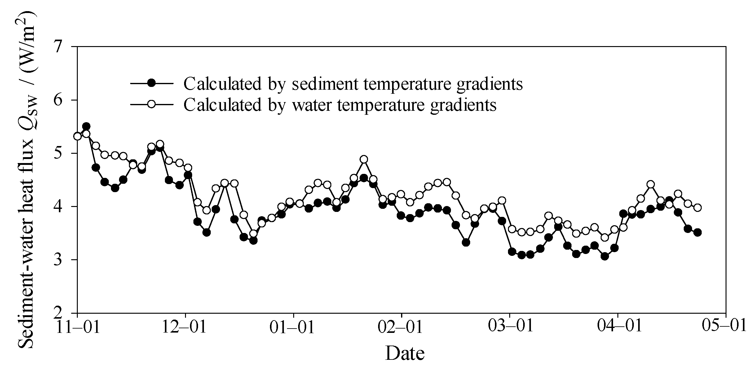
Figure 8 displays the temporal variations in sediment-water heat flux calculated through Equations (1) and (3) based on observational temperature data. As a comparison, Figure 8 shows the heat fluxes calculated by using both sediment temperature gradients and water temperature gradients. It can be seen from the figure that the two kinds of results both show that the sediment–water heat flux throughout the whole freezing duration remained as a positive value, implying that the sediment was releasing heat into the water. The sediment–water heat fluxes calculated using water temperature gradients are distributed in the range 3.4~5.3 W/m2, and the average value is 4.1 W/m2 during the whole freezing period, while the fluxes calculated by sediment temperature gradients are distributed in the range 3.5~4.6 W/m2, with an average of 3.8 W/m2. The average value calculated using the water temperature gradient is slightly larger than that by sediment temperature gradient, and the difference is 0.3 W/m2, which is equivalent to 7.3 and 7.9% of them, respectively.
Figure 9 demonstrates the temporal variations in water–ice heat flux at the water-ice interface calculated through Equation (4) based on the observational data temperature. As a comparison, Figure 9 also shows the heat fluxes calculated by using both ice temperature gradients and water temperature gradients. It can be seen from the figure that the two kinds of results both show that the water–ice heat flux throughout the whole freezing duration remained as a positive value, indicating that the water body was emitting heat into the ice cover. In addition, the two results both show the rising trend as time passed. The water–ice heat fluxes calculated using the water temperature gradients are distributed in the range 7.3–13.1 W/m2, and the average value is 10.3 W/m2 during the whole freezing period, while the fluxes calculated by ice temperature gradients are distributed in the range 6.9–12.1 W/m2, with an average of 9.8 W/m2. The average heat flux calculated using the water temperature gradient is also larger than that using the ice temperature gradient, and the difference is 0.5 W/m2, which is equivalent to 4.7 and 5.1% of them, respectively. The average value of water–ice heat flux, 9.8 or 10.3 W/m2, is greater than some results obtained in studies on deep lakes [40,41] (5–7 W/m2). Therefore, the calculation of ice thickness in a shallow lake would be far from reasonable if the water–ice heat transfer was neglected and the lower boundary of the ice cover was regarded as thermally isolated or observed values of the water–ice heat flux from a deep lake were adopted.
Overall, the average relative difference of heat flux calculated by using the temperature gradients on two sides of either interface is less than 7.9%. As it happens, the temperature observation operation was not very strictly controllable due to the limitation of natural conditions, and the average relative difference within 7.9% can be regarded as an insignificant statistical difference for the prototype observation. Therefore, the natural convection heat transfer process in water cannot be arbitrarily judged by the difference between the results of the two calculation methods. For the sediment–water heat flux, the average relative difference between the values calculated using the water side and either side is 7.9%, larger than that of water–ice heat flux, which might be due to the uncertainty of some of the parameters in the calculation of sediment thermal conductivity.
In addition, we found that the average value of sediment–water heat flux calculated by the sediment temperature gradient is 3.8 W/m2, and the average value of water–ice heat flux calculated using the ice temperature gradient is 9.8 W/m2, with a difference of 6 W/m2 (if the water temperature gradient is adopted, the difference is 6.2 W/m2). From the relationship between the two average values, the heat flux released by the water body from the water–ice interface to the ice is greater than the heat flux obtained by the water from the sediment–water interface. If only these two parts of the heat budget existed in water, the water temperature should continue to decrease with time, but as it can be seen from Figure 6, the water temperature increases gradually with the passage of time during the whole freezing duration. Therefore, there must be other heat sources to make up for the difference between Qsw and Qwi and supply additional heat to the water, so that the water temperature continues to rise. Obviously, the heat source is the solar radiation penetrating into the water. Next, the solar radiation penetrating into water during the freezing duration will be evaluated to verify the above hypothesis.
The solar radiation flux is related to latitude and date. According to the relevant meteorological research results [42], we obtained the variation process of the solar radiation flux in the prototype observation area, whose latitude is 45° N. Through a fitting regression, we developed an empirical expression of the solar radiation flux with the ordinal number of dates.
where Qrad is the solar radiation flux, W/m2; d is the ordinal number of the date, d on 1 January is 1, and d on 31 December of the previous year is −1; the application scope of Equation (13) is , i.e., from 1 October of the last year to 1 May of the next year.
The solar radiation will be reflected on the ice surface; therefore, the incident solar radiation flux from the ice surface is as follows:
where Qrad-ice is the incident solar radiation flux from the ice surface, W/m2; A is the albedo of ice, the value is about 0.5.
As part of Qrad-ice is absorbed by the ice, the solar radiation flux penetrating into the water is as follows:
where Qrad-water is the solar radiation flux penetrating into the water, W/m2; A is the albedo of the ice, the value is about 0.5; is the extinction coefficient of ice; and z is the ice thickness, m. In combination with Equations (13)–(15), the Qrad-water values during the freezing duration were calculated and are listed in Table 1.
It can be seen from Table 1 that in the whole freezing duration, the solar radiation flux penetrating into water is distributed in the range of 7.34–162.42 W/m2. Except for the large flux values in the initial period of ice formation and late ablation period, the average value of solar radiation flux in the stable sealing period (when the ice thickness is greater than 30 cm) is 12.48 W/m2, which is greater than the average value of the difference between Qwi and Qsw of 6–6.2 W/m2; therefore, the water temperature will continue to rise in the whole freezing duration.
3.5. Effective Thermal Diffusivity
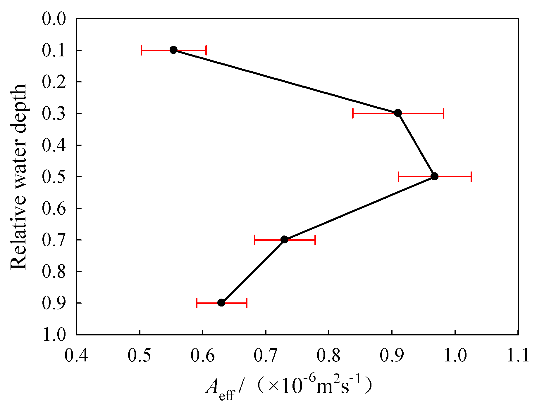
Figure 10 presents the calculated values of effective thermal diffusivity Aeff varied with water depths and time. It shows that the Aeff in water during the late winter was in the range of 0.32–1.37 × 10⁻⁶ m2/s, which was 2.3–9.8 times the molecular thermal diffusivity, amounting to 0.14 × 10⁻⁶ m2/s. Aeff varied with the position of relative water depth (Figure 10). Figure 11 is drawn based on the time-averaged values of Aeff at different water depths in late winter. It displays that the average value of Aeff in this period first increased and then decreased with relative water depth. The Aeff value in the middle relative depth was significantly larger, and the maximum value, 0.97 × 10⁻⁶ m2/s, occurred approximately at the relative depth of 0.5. It indicated that the water temperature in the mixed layer area tended to be more uniformly distributed since the natural convection there proved to be more drastic and water temperature spread more quickly between the different layers. In contrast, the water near the freezing front (conduction layer) and near sediment (quiescent layer) had larger vertical temperature gradients and the temperatures were more inhomogeneously distributed in comparison to the mixed layer, due to the small effective thermal diffusivities and slow spread of water temperature.
4. Conclusions
In this study, a field observation of Qinghuahu Lake, a typical ice-covered shallow lake of Heilongjiang Province, was carried out to clarify the thermal conditions of icebound water. The temporal variations and vertical profile patterns of water temperature throughout the ice-cover duration were analyzed, and heat fluxes at interfaces and effective thermal diffusivity inside the water were, thus, evaluated based on temperature data.
The temporal variation and vertical distribution of the water temperature in the frozen shallow lake are obviously affected by the process of the ice’s growth and decay. The whole ice duration can be divided into three different periods according to ice thickness to analyze the water temperature, i.e., ice formation period, stable freezing period, and late winter. During the initial stage of the ice formation period, the vertical gradient of the water temperature is small. With the gradual thickening of the ice cover, the overall water temperature and gradient increase. In the stable freezing period, vertical water profile is approximately linear. During late winter, the vertical profile of water temperature presents a typical three-layer structure, namely, a conduction layer, a mixed layer, and a quiescent layer. The thickness of the three layers varies with time. The maximum diurnal difference of water temperature, amounting to 1.4 K, appears in the transition zone between the conduction layer and the mixed layer.
Based on the observed temperature data, the heat fluxes at the water–ice interface and the sediment–water interface were evaluated. The sediment–water heat flux and water–ice heat flux both remain in positive values throughout the freezing duration, and the average relative difference of heat flux calculated by using the temperature gradients on both sides of either interface is less than 7.9%. The average difference between the water–ice heat flux and the sediment–water heat flux is about 6~6.2 W/m2, while the averaged flux of solar radiation penetrating into the water is at least 12.48 W/m2, which is larger than 6~6.2 W/m2; therefore, the water temperature continues to rise in the whole freezing duration. The results also demonstrate that the thermal structure of extremely shallow lakes follows the same seasonal pattern of water temperature dynamics as in lakes with a relatively larger depth.
A model solving effective thermal diffusivity based on temperature data was established, and the calculated effective thermal diffusivity is about 2.3–9.8 times the molecular thermal diffusivity, and the time-averaged values first increase and then decrease with the relative water depth, reaching a maximum at the relative depth of 0.5, which indicates that the water temperature of a mixed layer tends to be more uniformly distributed than that of a conduction layer and a quiescent layer.
Author Contributions
Conceptualization, F.D. and Z.M.; methodology, F.D. and Z.M.; writing—original draft preparation, F.D.; writing—review and editing, F.D. and Z.M. All authors have read and agreed to the published version of the manuscript.
Funding
This research received no external funding.
Conflicts of Interest
The authors declare no conflict of interest.
References
- Zhang, Y.L.; Chen, W.M.; Yang, D.T.; Huang, W.Y.; Jiang, J. Monitoring and analysis of thermodynamics in Tianmuhu Lake. ShuikexueJinzhan/Adv. Water Sci. 2004, 15, 61–67. [Google Scholar] [CrossRef]
- Zhu, S.; Ptak, M.; Yaseen, Z.M.; Dai, J.; Sivakumar, B. Forecasting surface water temperature in lakes: A comparison of approaches. J. Hydrol. 2020, 585, 124809–124818. [Google Scholar] [CrossRef]
- Bachmann, R.W.; Canfield, D.E.; Sharma, S.; Lecours, V. Warming of near-surface summer water temperatures in lakes of the conterminous united states. Water 2020, 12, 3381. [Google Scholar] [CrossRef]
- Ptak, M.; Sojka, M.; Choiński, A.; Nowak, B. Effect of environmental conditions and morphometric parameters on surface water temperature in Polish lakes. Water 2018, 10, 580. [Google Scholar] [CrossRef] [Green Version]
- Ptak, M.; Tomczyk, A.M.; Wrzesinski, D. Effect of teleconnection patterns on changes in water temperature in Polish lakes. Atmosphere 2018, 9, 66. [Google Scholar] [CrossRef] [Green Version]
- Yang, K.; Yu, Z.; Luo, Y.; Yang, Y.; Zhao, L.; Zhou, X. Spatial and temporal variations in the relationship between lake water surface temperatures and water quality—A case study of Dianchi Lake. Sci. Total Environ. 2018, 624, 859–871. [Google Scholar] [CrossRef] [PubMed]
- Wang, S. Freezing Temperature Controls Winter Water Discharge for Cold Region Watershed. Water Resour. Res. 2019, 55, 10051–11354. [Google Scholar] [CrossRef] [Green Version]
- Gronewold, A.D.; Anderson, E.J.; Lofgren, B.; Blanken, P.D.; Wang, J.; Smith, J.; Hunter, T.; Lang, G.; Stow, C.A.; Beletsky, D.; et al. Impacts of extreme 2013–2014 winter conditions on Lake Michigan’s fall heat content, surface temperature, and evaporation. Geophys. Res. Lett. 2015, 42, 3364–3370. [Google Scholar] [CrossRef] [Green Version]
- Iestyn Woolway, R.; Merchant, C.J. Amplified surface temperature response of cold, deep lakes to inter-annual air temperature variability. Sci. Rep. 2017, 7, 4130–4138. [Google Scholar] [CrossRef] [Green Version]
- Yang, F.; Li, C.; Shi, X.; Zhao, S.; Hao, Y. Impact of seasonal ice structure characteristics on ice cover impurity distributions in Lake Ulansuhai. HupoKexue/J. Lake Sci. 2016, 28, 455–462. [Google Scholar] [CrossRef] [Green Version]
- Kirillin, G.; Leppäranta, M.; Terzhevik, A.; Granin, N.; Bernhardt, J.; Engelhardt, C.; Efremova, T.; Golosov, S.; Palshin, N.; Sherstyankin, P.; et al. Physics of seasonally ice-covered lakes: A review. Aquat. Sci. 2012, 74, 659–682. [Google Scholar] [CrossRef]
- Zhou, C.; Liang, R.; Xiao, Y.; Li, K. Water temperature and ice conditions of high-dam reservoirs in northwestern cold and arid regions. ShuiliFadianXuebao/J. Hydroelectr. Eng. 2016, 35, 31–39. [Google Scholar] [CrossRef]
- Teng, H.; Deng, Y.; Huang, F.B.; Tuo, Y.C. Experimental study on the simulation of freezing processes in calm waters and thermal changes on reservoir ice cover. ShuikexueJinzhan/Adv. Water Sci. 2011, 22, 720–726. [Google Scholar] [CrossRef] [Green Version]
- Ulloa, H.N.; Winters, K.B.; Wüest, A.; Bouffard, D. Differential Heating Drives Downslope Flows that Accelerate Mixed-Layer Warming in Ice-Covered Waters. Geophys. Res. Lett. 2019, 46, 13872–13882. [Google Scholar] [CrossRef] [Green Version]
- Frassl, M.A.; Boehrer, B.; Holtermann, P.L.; Hu, W.; Klingbeil, K.; Peng, Z.; Zhu, J.; Rinke, K. Opportunities and limits of using meteorological reanalysis data for simulating seasonal to sub-daily water temperature dynamics in a large shallow lake. Water 2018, 10, 594. [Google Scholar] [CrossRef] [Green Version]
- Williams, P.; Whitfield, M.; Biggs, J.; Bray, S.; Fox, G.; Nicolet, P.; Sear, D. Comparative biodiversity of rivers, streams, ditches and ponds in an agricultural landscape in Southern England. Biol. Conserv. 2004, 115, 329–341. [Google Scholar] [CrossRef]
- Downing, J.A. Emerging global role of small lakes and ponds: Little things mean a lot. Limnetica 2010, 29, 9–24. [Google Scholar] [CrossRef]
- Huang, W.; Han, H.; Niu, F.; Li, Z. Field observations on water temperature and stratification in a seasonally ice-covered shallow thermokarst lake. ShuikexueJinzhan/Adv. Water Sci. 2016, 27, 280–289. [Google Scholar] [CrossRef]
- de la Fuente, A.; Meruane, C. Dimensionless numbers for classifying the thermodynamics regimes that determine water temperature in shallow lakes and wetlands. Environ. Fluid Mech. 2017, 17, 1081–1098. [Google Scholar] [CrossRef]
- Torma, P.; Wu, C.H. Temperature and circulation dynamics in a small and shallow lake: Effects of weak stratification and littoral submerged macrophytes. Water 2019, 11, 128. [Google Scholar] [CrossRef] [Green Version]
- Bouffard, D.; Zdorovennov, R.E.; Zdorovennova, G.E.; Pasche, N.; Wüest, A.; Terzhevik, A.Y. Ice-covered Lake Onega: Effects of radiation on convection and internal waves. Hydrobiologia 2016, 780, 1–16. [Google Scholar] [CrossRef]
- Hamilton, D.P.; Magee, M.R.; Wu, C.H.; Kratz, T.K. Ice cover and thermal regime in a dimictic seepage lake under climate change. Inl. Waters 2018, 8, 381–398. [Google Scholar] [CrossRef]
- Zhao, L.L.; Zhu, G.W.; Chen, Y.F.; Li, W.; Zhu, M.Y.; Yao, X.; Cai, L.L. Thermal stratification and its influence factors in a large-sized and shallow Lake Taihu. ShuikexueJinzhan/Adv. Water Sci. 2011, 22, 844–850. [Google Scholar] [CrossRef]
- Huang, W.; Cheng, B.; Zhang, J.; Zhang, Z.; Vihma, T.; Li, Z.; Niu, F. Modeling experiments on seasonal lake ice mass and energy balance in Qinghai-Tibet Plateau: A case study. Hydrol. Earth Syst. Sci. Discuss. 2018, 23, 1–25. [Google Scholar] [CrossRef] [Green Version]
- Yang, F.; Feng, W.; Matti, L.; Yang, Y.; Merkouriadi, I.; Cen, R.; Bai, Y.; Li, C.; Liao, H. Simulation and seasonal characteristics of the intra-annual heat exchange process in a shallow ice-covered lake. Sustainability 2020, 12, 7832. [Google Scholar] [CrossRef]
- Song, K.; Wen, Z.; Jacinthe, P.A.; Zhao, Y.; Du, J. Dissolved carbon and CDOM in lake ice and underlying waters along a salinity gradient in shallow lakes of Northeast China. J. Hydrol. 2019, 571, 545–558. [Google Scholar] [CrossRef] [Green Version]
- Liu, R.; Bao, K.; Yao, S.; Yang, F.; Wang, X. Ecological risk assessment and distribution of potentially harmful trace elements in lake sediments of Songnen Plain, NE China. Ecotoxicol. Environ. Saf. 2018, 163, 117–124. [Google Scholar] [CrossRef]
- Fang, X.; Stefan, H.G. Dynamics of heat exchange between sediment and water in a lake. Water Resour. Res. 1996, 32, 1719–1727. [Google Scholar] [CrossRef]
- Birge, E.; Juday, C.; March, H. The Temperature of the Bottom Deposits of Lake Mendota, A Chapter in the Heat Exchanges of the Lake. Trans. Wis. Acad. Sci. Arts Lett. 1927, 23, 187–231. [Google Scholar]
- Pivovarov, A.A. Thermal Conditions in Freezing Lakes and Rivers; Wiley: New York, NY, USA, 1973. [Google Scholar]
- Ryanzhin, S.V. Thermophysical Properties of Lake Sediments and Water-Sediments Heat Interaction; Repo~No. 3214; Department of Water Resources Engineering, Institute of Technology, University of Lund: Lund, Sweden, 1997. [Google Scholar]
- Yang, S.M.; Tao, W.Q. Heat Transfer, 4th ed.; Higher Education Press: Beijing, China, 2006; p. 272. [Google Scholar]
- Petrov, M.P.; Terzhevik, A.Y.; Zdorovennov, R.E.; Zdorovennova, G.E. The thermal structure of a shallow lake in early winter. Water Resour. 2006, 33, 135–143. [Google Scholar] [CrossRef]
- Aslamov, I.A.; Kozlov, V.V.; Misandrontsev, I.B.; Kucher, K.M.; Granin, N.G. Estimate of heat flux at the ice-water interface in Lake Baikal from experimental data. Dokl. Earth Sci. 2014, 457, 982–985. [Google Scholar] [CrossRef]
- Zeng, Y.; Zhu, J.; Wang, Y.; Hu, W. Changes of water temperature and heat flux at water-sediment interface, East Lake Taihu. HupoKexue/J. Lake Sci. 2018, 30, 1599–1609. [Google Scholar] [CrossRef] [Green Version]
- Chapman, A.J. Heat transfer. Magn. Reson. Mater. Biol. Phys. Med. 1974, 9, 146–151. [Google Scholar] [CrossRef] [PubMed]
- Jakkila, J.; Leppäranta, M.; Kawamura, T.; Shirasawa, K.; Salonen, K. Radiation transfer and heat budget during the ice season in Lake Pääjärvi, Finland. Aquat. Ecol. 2009, 43, 681–692. [Google Scholar] [CrossRef]
- Kirillin, G.; Terzhevik, A. Thermal instability in freshwater lakes under ice: Effect of salt gradients or solar radiation? Cold Reg. Sci. Technol. 2011, 65, 184–190. [Google Scholar] [CrossRef]
- Leppäranta, M.; Terzhevik, A.; Shirasawa, K. Solar radiation and ice melting in Lake vendyurskoe, Russian Karelia. Hydrol. Res. 2010, 41, 50–62. [Google Scholar] [CrossRef]
- Aslamov, I.A.; Kozlov, V.V.; Kirillin, G.B.; Mizandrontsev, I.B.; Kucher, K.M.; Makarov, M.M.; Gornov, A.Y.; Granin, N.G. Ice-water heat exchange during ice growth in Lake Baikal. J. Great Lakes Res. 2014, 40, 599–607. [Google Scholar] [CrossRef]
- Bengtsson, L.; Svensson, T. Thermal regime of ice covered Swedish lakes. Hydrol. Res. 1996, 27, 39–56. [Google Scholar] [CrossRef]
- Jolliffe, I.T.; Stephenson, D.B. Forecast Verification: A Practitioner’s Guide in Atmospheric Science, 2nd ed.; Forecast Verification; Wiley & Sons: Chichester, UK, 2012. [Google Scholar]
Figure 1.
Observation site and schematic diagram of layout. (a) Observation site, (b) Schematic diagram of temperature chain layout.
Figure 1.
Observation site and schematic diagram of layout. (a) Observation site, (b) Schematic diagram of temperature chain layout.
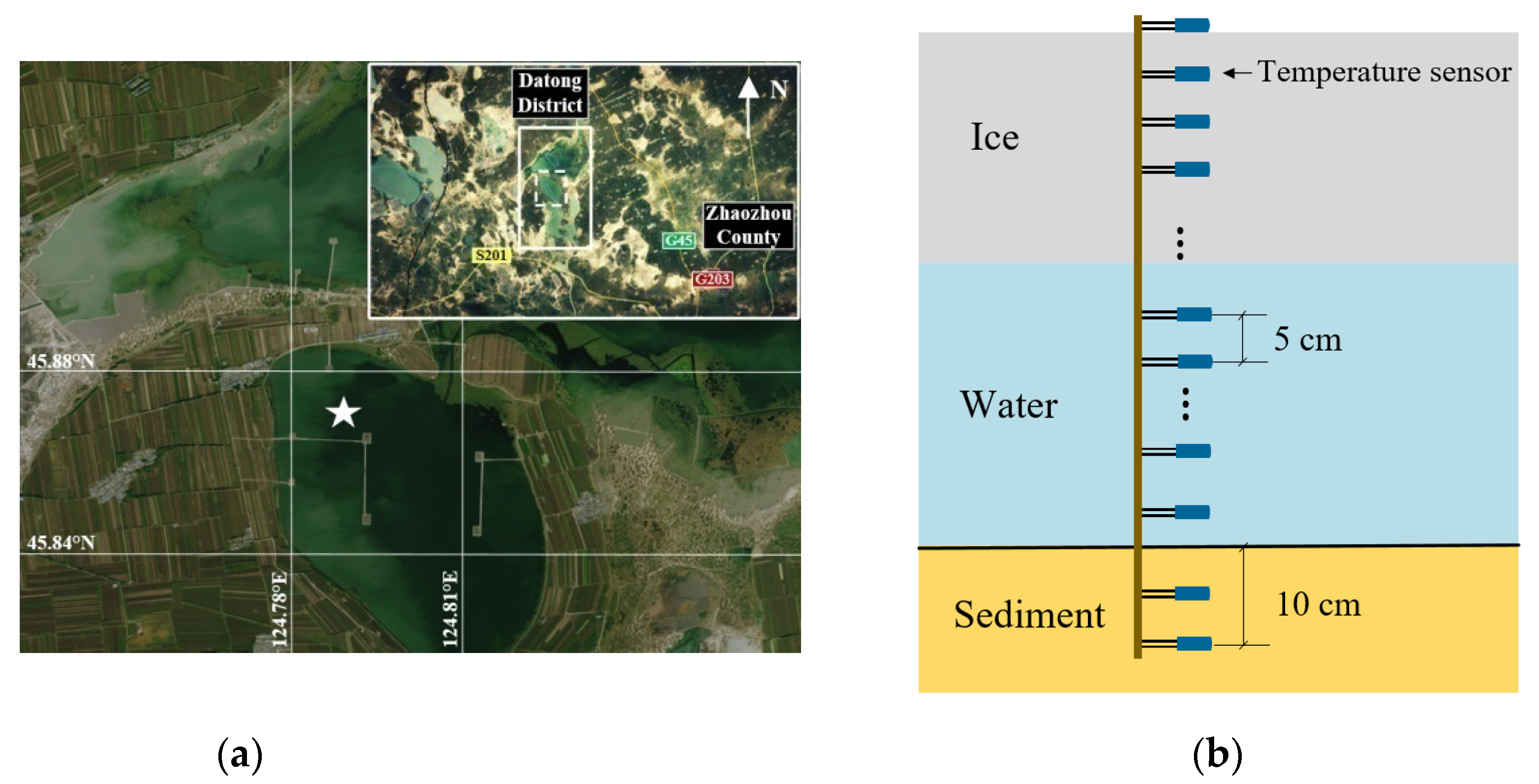
Figure 2.
Schematic diagram concerning the calculation of effective thermal diffusivity.
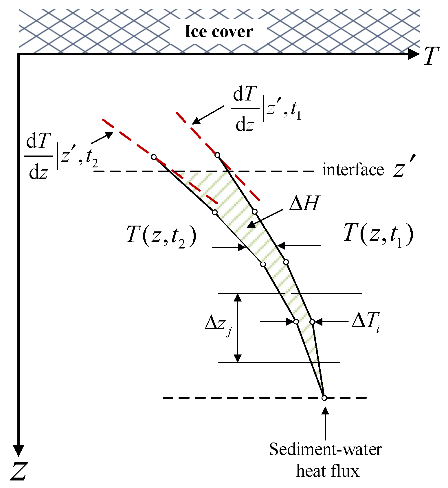
Figure 3.
The processes of lake ice growing and melting (short dash lines are the sensors’ horizontal planes).
Figure 3.
The processes of lake ice growing and melting (short dash lines are the sensors’ horizontal planes).
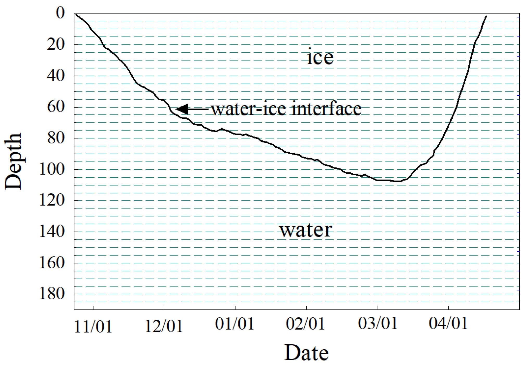
Figure 4.
Variations in water temperature beneath the ice during the first 3 days of ice formation.
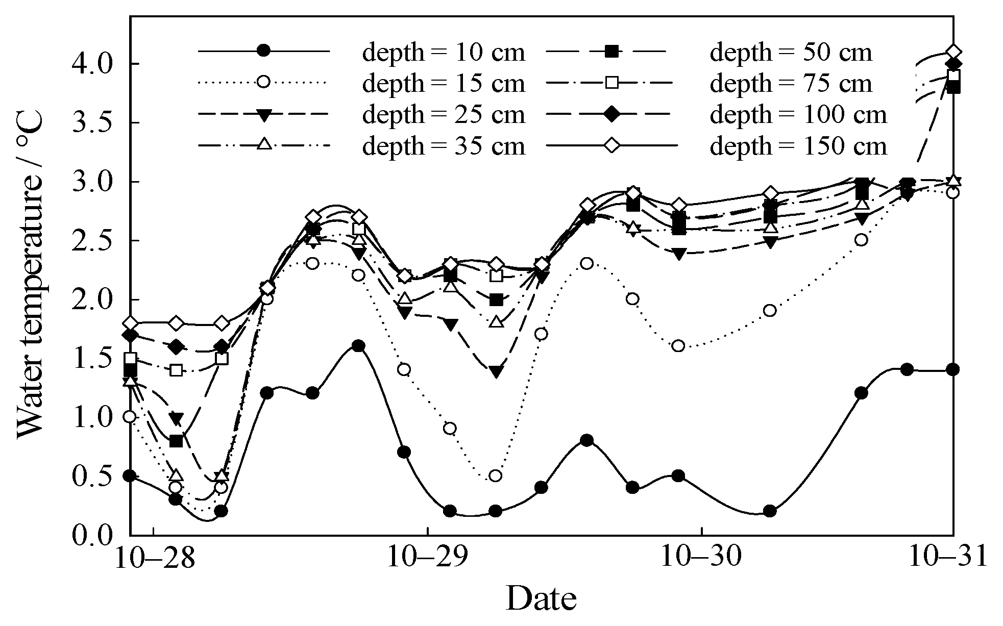
Figure 5.
Variations of water temperatures during the late winter.

Figure 6.
Vertical profiles of water temperature in the ice-cover duration.
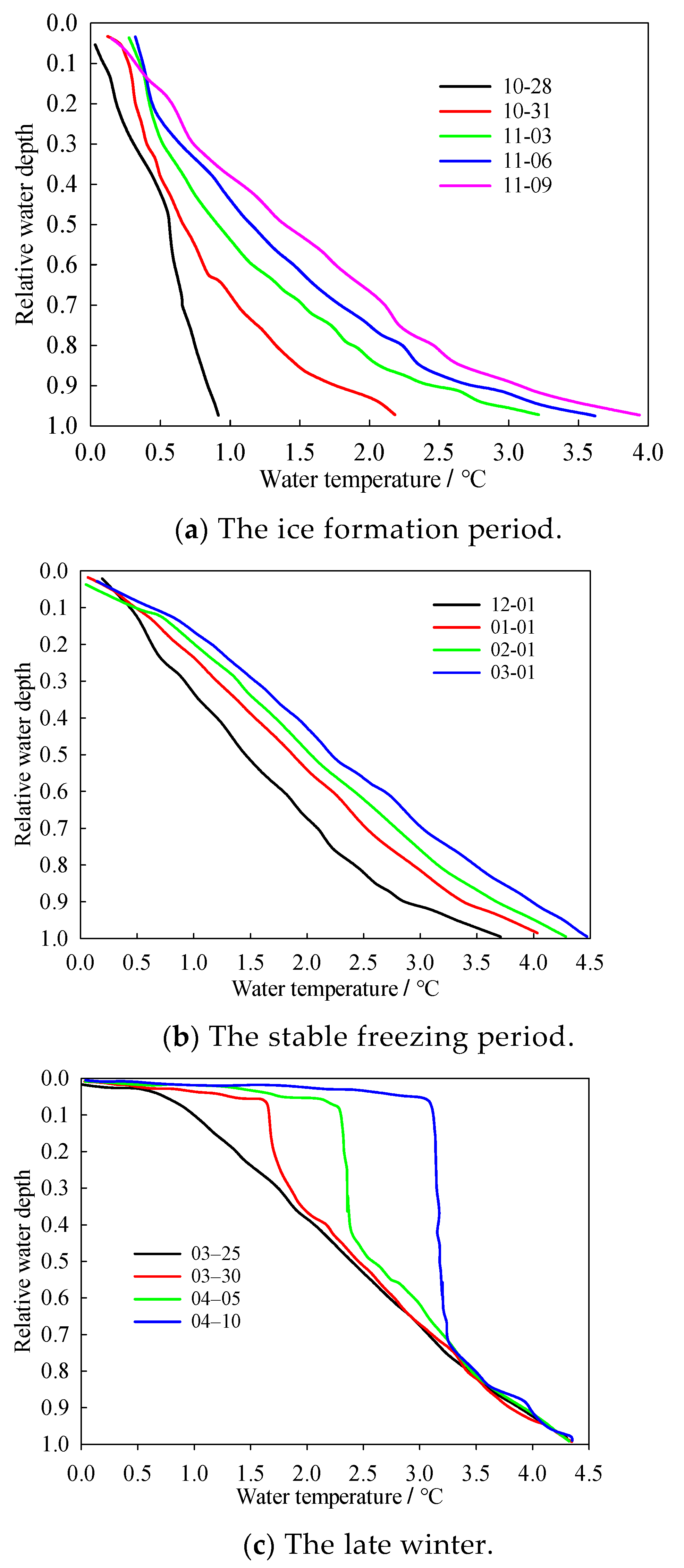
Figure 7.
Diurnal variations in the vertical profiles of water temperature during the late winter.
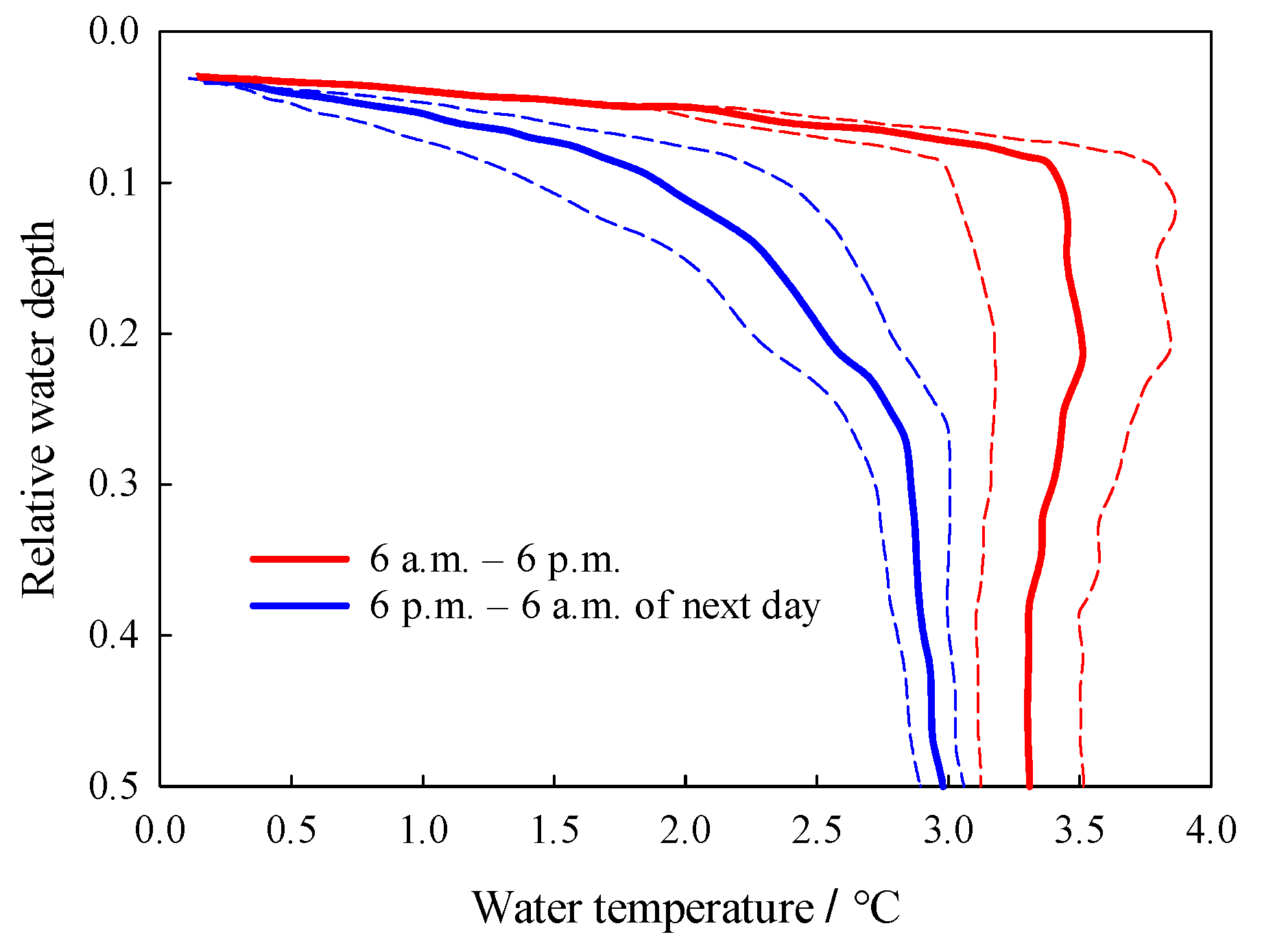
Figure 8.
Seasonal variations in sediment–water heat flux over the ice-cover duration.

Figure 9.
Seasonal variations in water–ice heat flux over the ice-cover duration.
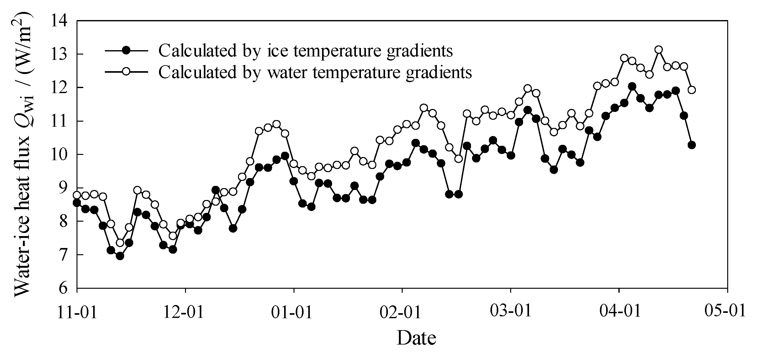
Figure 10.
Calculated values of effective thermal diffusivity changed with depth and date of late winter.
Figure 10.
Calculated values of effective thermal diffusivity changed with depth and date of late winter.
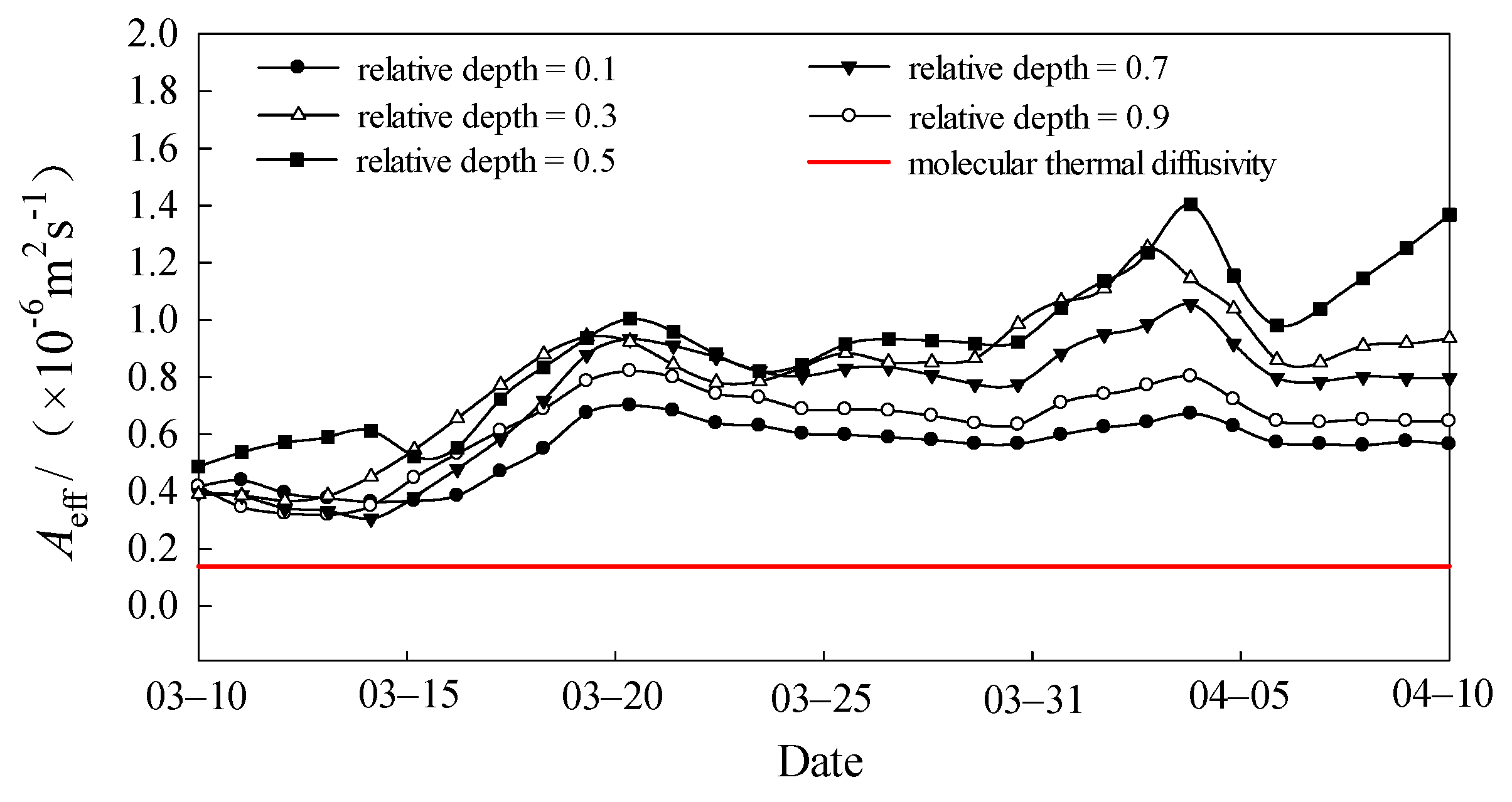
Figure 11.
Time-averaged vertical profile of effective thermal diffusivity in late winter.

Table 1.
Seasonal variations of solar radiation flux penetrating into water.
| Date | d | Qrad (W/m2) | Qrad-ice (W/m2) | z (m) | Qrad-water (W/m2) |
|---|---|---|---|---|---|
| 11/1 | −61 | 183.34 | 91.67 | 0.07 | 76.95 |
| 11/6 | −56 | 167.73 | 83.87 | 0.15 | 57.64 |
| 11/11 | −51 | 154.14 | 77.07 | 0.24 | 42.30 |
| 11/16 | −46 | 142.47 | 71.23 | 0.31 | 32.82 |
| 11/21 | −41 | 132.65 | 66.33 | 0.43 | 22.64 |
| 11/26 | −36 | 124.62 | 62.31 | 0.47 | 19.24 |
| 12/1 | −31 | 118.29 | 59.14 | 0.54 | 15.33 |
| 12/6 | −26 | 113.59 | 56.80 | 0.63 | 11.76 |
| 12/11 | −21 | 110.45 | 55.22 | 0.67 | 10.34 |
| 12/16 | −16 | 108.78 | 54.39 | 0.70 | 9.45 |
| 12/21 | −11 | 108.52 | 54.26 | 0.74 | 8.53 |
| 12/26 | −6 | 109.59 | 54.80 | 0.75 | 8.40 |
| 1/1 | 1 | 113.19 | 56.59 | 0.76 | 8.46 |
| 1/6 | 6 | 117.14 | 58.57 | 0.76 | 8.76 |
| 1/11 | 11 | 122.17 | 61.09 | 0.79 | 8.48 |
| 1/16 | 16 | 128.21 | 64.10 | 0.82 | 8.25 |
| 1/21 | 21 | 135.16 | 67.58 | 0.85 | 8.07 |
| 1/26 | 26 | 142.97 | 71.49 | 0.88 | 7.92 |
| 2/1 | 32 | 153.36 | 76.68 | 0.92 | 7.69 |
| 2/6 | 37 | 162.77 | 81.38 | 0.94 | 7.76 |
| 2/11 | 42 | 172.79 | 86.40 | 0.96 | 7.84 |
| 2/16 | 47 | 183.35 | 91.67 | 1.01 | 7.34 |
| 2/21 | 52 | 194.37 | 97.18 | 1.03 | 7.40 |
| 2/26 | 57 | 205.77 | 102.89 | 1.04 | 7.64 |
| 3/1 | 60 | 212.77 | 106.38 | 1.05 | 7.71 |
| 3/6 | 65 | 224.63 | 112.31 | 1.05 | 8.14 |
| 3/11 | 70 | 236.68 | 118.34 | 1.05 | 8.57 |
| 3/16 | 75 | 248.85 | 124.43 | 1.02 | 9.72 |
| 3/21 | 80 | 261.06 | 130.53 | 0.94 | 12.45 |
| 3/26 | 85 | 273.23 | 136.62 | 0.86 | 15.91 |
| 4/1 | 91 | 287.69 | 143.84 | 0.71 | 24.38 |
| 4/6 | 96 | 299.52 | 149.76 | 0.52 | 40.81 |
| 4/11 | 101 | 311.08 | 155.54 | 0.24 | 85.36 |
| 4/16 | 106 | 322.28 | 161.14 | 0.08 | 131.93 |
| 4/21 | 111 | 333.06 | 166.53 | 0.01 | 162.42 |
Publisher’s Note: MDPI stays neutral with regard to jurisdictional claims in published maps and institutional affiliations. |
© 2021 by the authors. Licensee MDPI, Basel, Switzerland. This article is an open access article distributed under the terms and conditions of the Creative Commons Attribution (CC BY) license (https://creativecommons.org/licenses/by/4.0/).
Share and Cite
MDPI and ACS Style
Ding, F.; Mao, Z. Observation and Analysis of Water Temperature in Ice-Covered Shallow Lake: Case Study in Qinghuahu Lake. Water 2021, 13, 3139. https://doi.org/10.3390/w13213139
AMA Style
Ding F, Mao Z. Observation and Analysis of Water Temperature in Ice-Covered Shallow Lake: Case Study in Qinghuahu Lake. Water. 2021; 13(21):3139. https://doi.org/10.3390/w13213139
Chicago/Turabian StyleDing, Falong, and Zeyu Mao. 2021. "Observation and Analysis of Water Temperature in Ice-Covered Shallow Lake: Case Study in Qinghuahu Lake" Water 13, no. 21: 3139. https://doi.org/10.3390/w13213139
Note that from the first issue of 2016, this journal uses article numbers instead of page numbers. See further details here.